Highlights
What are the main findings?
- The spatio-temporal correlation-aware deep learning network for LAI inversion, STC-DeepLAINet, outperforms eight widely used machine learning methods as well as state-of-the-art deep learning methods across all three quantitative metrics: R2, RMSE, and bias.
- Compared to the mainstream GLASS LAI product (prone to saturation in high LAI scenarios), STC-DeepLAINet generates LAI products with superior consistency with ground-based measurements, addressing a critical limitation of existing LAI inversion products.
What are the implications of the main findings?
- This work provides an operational framework for large-scale high-precision LAI product generation, supporting agricultural yield estimation and ecosystem carbon cycle simulation in China.
- The integration of Transformer and GCN in STC-DeepLAINet offers a new paradigm for capturing long-range spatio-temporal dependencies, advancing deep learning applications in ecological remote sensing.
Abstract
Leaf area index (LAI) is a pivotal biophysical parameter linking vegetation physiological processes and macro-ecological functions. Accurate large-scale LAI estimation is indispensable for agricultural management, climate change research, and ecosystem modeling. However, existing methods fail to efficiently extract integrated spatial-spectral-temporal features and lack targeted modeling of spatio-temporal dependencies, compromising the accuracy of LAI products. To address this gap, we propose STC-DeepLAINet, a Transformer-GCN hybrid deep learning architecture integrating spatio-temporal correlations via the following three synergistic modules: (1) a 3D convolutional neural networks (CNNs)-based spectral-spatial embedding module capturing intrinsic correlations between multi-spectral bands and local spatial features; (2) a spatio-temporal correlation-aware module that models temporal dynamics (by “time periods”) and spatial heterogeneity (by “spatial slices”) simultaneously; (3) a spatio-temporal pattern memory attention module that retrieves historically similar spatio-temporal patterns via an attention-based mechanism to improve inversion accuracy. Experimental results demonstrate that STC-DeepLAINet outperforms eight state-of-the-art methods (including traditional machine learning and deep learning networks) in a 500 m resolution LAI inversion task over China. Validated against ground-based measurements, it achieves a coefficient of determination (R2) of 0.827 and a root mean square error (RMSE) of 0.718, outperforming the GLASS LAI product. Furthermore, STC-DeepLAINet effectively captures LAI variability across typical vegetation types (e.g., forests and croplands). This work establishes an operational solution for generating large-scale high-precision LAI products, which can provide reliable data support for agricultural yield estimation and ecosystem carbon cycle simulation, while offering a new methodological reference for spatio-temporal correlation modeling in remote sensing inversion.
1. Introduction
Vegetation is a fundamental and irreplaceable part of the global land surface system, playing a decisive role in maintaining the global energy equilibrium and mitigating the impacts of climate change. Precise inversion of vegetation biophysical parameters is thus of utmost importance for effectively monitoring vegetation growth dynamics [1,2]. Among these parameters, the leaf area index (LAI), defined as half of the total green leaf area per unit horizontal ground surface, is pivotal for numerous key applications. These applications range from accurate crop yield forecasting, which is crucial for global food security, to precise carbon cycle quantification, and in-depth climate change impact assessment [3,4]. Its spatio-temporal dynamics directly affect the accuracy of land surface models used for climate projections, as highlighted in the Intergovernmental Panel on Climate Change (IPCC) 2022 reports [5]. Ground-based observations, while accurate at local scales, struggle to provide spatially continuous LAI measurements across large regions. Thus, deriving large-scale LAI products with spatio-temporal correlations from multidimensional satellite data has become a critical approach to address this limitation [6].
Currently, the most widely used LAI products including MODIS LAI and GLASS LAI suffered from non-negligible limitations that restricted their application in precise ecosystem monitoring. For example, the MODIS LAI product has been reported to exhibit inconsistencies across different biomes, with a notable underestimation in tropical regions. This is mainly due to its algorithm’s inability to adapt well to the unique vegetation characteristics in these areas [7]. The GLASS LAI product exhibits a saturation effect when compared with ground-based LAI measurements, particularly in high LAI scenarios (e.g., forest vegetation types) [8]. This saturation problem has been deeply rooted in the limitations of the remote sensing-based LAI inversion approaches used in its development, highlighting the urgent need to optimize existing inversion methods. To date, remote sensing-based LAI inversion has been extensively explored using the following three primary approaches: empirical statistical models, physical models, and machine learning models [9,10]. Empirical statistical models, however, fail to capture spatio-temporal correlations across large areas due to their inherent dependence on local calibration datasets, which restricts their applicability beyond the inversion area [11]. Physical models, such as those used to generate the Moderate Resolution Imaging Spectroradiometer (MODIS) LAI product, resolve mechanistic processes and support global applications—this product has been widely adopted for vegetation and ecosystem dynamic monitoring and modeling [12]. Nevertheless, physical models often face ill-posed inversion problems: even with reasonable estimates under specific conditions, radiation transfer models (a typical type of physical model) produce a set of possible LAI solutions rather than a unique value, constrained by observational conditions [13].
Machine learning has substantially improved LAI inversion accuracy by avoiding the limitations of empirical statistical models, physical models [14,15], but traditional machine learning models—such as random forest (RF) and Generalized Regression Neural Networks (GRNNs)—require manually designed domain-specific features and cannot proactively extract effective spatio-temporal correlation information from multidimensional data [16]. Although emerging deep learning techniques like Long Short-Term Memory (LSTM) networks and 3D convolutional neural networks (3D CNNs) show promise in LAI inversion, they also have their own limitations. Three-dimensional CNNs are effective at extracting local spatial texture features within pixel neighborhoods but struggle to model long-distance spatial correlations due to the complex and diverse nature of vegetation distribution [17,18,19]. LSTM networks, when processing ultra-long time series, often fail to capture cross-year climate cycle patterns because of memory attenuation [20].
To bridge these gaps, a novel deep learning framework capable of autonomously capturing large-scale spatio-temporal correlations is needed to further improve the accuracy of remote sensing-based LAI inversion. In computer vision and natural language processing, Transformer architectures have demonstrated exceptional performance in modeling long-term temporal dependencies [21]. Unlike recurrent networks, the Transformer’s self-attention mechanism reduces the effective path length of temporal signals to O(1), enabling parallel computation and efficient capture of both short- and long-range temporal dependencies—a key advantage for addressing the memory attenuation issue of LSTMs in ultra-long time series LAI inversion [22]. Graph Convolutional Networks (GCNs), on the other hand, model spatial topological structures through neighborhood-based feature aggregation [23], providing a principled approach to encode geospatial relationships and overcome the long-distance spatial correlation limitation of 3D CNNs [24,25].
Building on this foundation, we proposed Spatio-temporal Correlation DeepLAINet (STC-DeepLAINet)—a Transformer-GCN hybrid architecture specifically designed to capture the inherent spatio-temporal correlations in LAI dynamics, it offers a novel solution to the long-standing problems in LAI inversion by integrating the strengths of Transformer-based temporal modeling and GCN-based spatial representation. This integrated approach was verified to be based on the LAI inversion task with a resolution of 500 m across China. The main contributions of this work are as follows:
- A spatio-temporal correlation attention framework is proposed, integrating Transformer-based temporal correlation mining and GCN-based spatial similarity modeling to address the limitation of capturing long-range spatio-temporal dependencies. By correlating time periods (not discrete points) and spatial slices (not pixels), it improves identifying complex spatio-temporal pattern dependencies.
- An attention-driven spatio-temporal pattern memory mechanism was designed to adaptively retrieve and leverage historically similar patterns while fusing spatio-temporal features, thereby improving LAI inversion accuracy and making it particularly suitable for complex vegetation ecosystems.
- A novel knowledge-guided loss function is designed to directly constrain the LAI inversion process, mitigating the saturation effect in LAI inversion and yielding high-precision, large-scale LAI products that offer reliable data support to agricultural and ecological research.
The remainder of this paper is organized as follows. Section 2 describes the remote sensing products used and the dataset construction process. Section 3 details the proposed STC-DeepLAINet architecture, experimental settings, and comparison methods. Section 4 presents the experimental results, including performance comparisons with competing methods, module ablation studies, hyperparameter analysis, and validation of the generated LAI products. Section 5 discusses the network’s limitations and future improvement directions. Finally, Section 6 draws the conclusions of this study.
2. Materials
2.1. Study Area
In this study, the proposed STC-DeepLAINet framework was validated across China, which covers approximately 9.6 million square kilometers (3°51′–53°33′N, 73°33′–135°05′E), spans tropical to temperate zones, encompassing complex terrains (plateaus, basins, plains) and diverse vegetation types (forests, grasslands, shrublands, croplands, deserts). The vast territory provides a natural study case for LAI inversion across environmental gradients. Figure 1 is derived from the 2024 MODIS Land Cover Type product (MCD12Q1.061) [26].
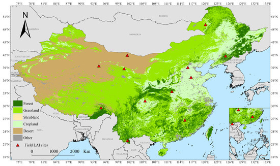
Figure 1.
Spatial distribution of vegetation types across China.
2.2. Data Description and Processing
- (1)
- MODIS LAI
The MODIS LAI product (MOD15A2H) features a spatial resolution of 500 m and a temporal resolution of 8 days. Its retrieval algorithm is primarily based on three-dimensional radiative transfer model, from which a biome-specific Look-Up Table is generated to match satellite-observed surface reflectance [12].
- (2)
- VIIRS LAI
The VIIRS LAI (VNP15A2H) algorithm inherits the advantages of the MODIS algorithm, maintaining a spatial resolution of 500 m and a temporal resolution of 8 days. It employed an improved atmospheric correction algorithm, which effectively reduced cloud and atmospheric interference [27].
- (3)
- GLASS LAI V6
The GLASS V6 product was derived using a Bidirectional Long Short-Term Memory (Bi-LSTM) network. This network first performed temporal smoothing on surface reflectance data prior to network training, thereby enhancing the spatio-temporal consistency of the resulting LAI product [8].
- (4)
- MODIS Surface Reflectance Product
The MODIS surface reflectance product (MOD09A1) product delivered surface reflectance across seven spectral bands (Table 1) and also provided per-pixel geometric parameters along with quality assurance layers essential for atmospheric correction [28].

Table 1.
Specifications of seven spectral bands in the MODIS MOD09A1 product.
- (5)
- Ground-based LAI measurements
To directly validate the inverted LAI against ground-based measurements, we collected ground-based observations of LAI from 12 sites from 2022 to 2024. These data were obtained from the following three sources: (1) the National Ecosystem Science Data Center, National Science and Technology Infrastructure of China (available at http://www.nesdc.org.cn), (2) the National Tibetan Plateau Data Center (available at http://data.tpdc.ac.cn), and (3) ground-based LAI conducted by our research team using the LAI-2200 Plant Canopy Analyzer (Li-Cor Biosciences, Lincoln, NE, USA). The spatial distribution of these 12 sampling sites is illustrated in Figure 1, with detailed site information provided in Appendix A Table A1 [29].
- (6)
- Data preprocessing
To prepare reliable inputs for STC-DeepLAINet, the remote sensing products underwent preprocessing as follows: MODIS, VIIRS, and GLASS LAI products were reshaped to 32 × 32 × 1 arrays (label datasets), while the MOD09A1 surface reflectance product was formatted to 32 × 32 × 7 arrays (feature datasets), where 1 and 7 denote the band counts for LAI and reflectance, respectively. For LAI label integration, given that MODIS LAI products lack preprocessing or post-processing for cloud-contaminated pixels and exhibit greater fluctuation than VIIRS and GLASS LAI, multi-source products were combined as follows: if VIIRS and GLASS LAI differed by <1 unit, their average was used; otherwise, the median of MODIS, VIIRS, and GLASS LAI was adopted, with GLASS LAI as fallback when MODIS/VIIRS data were invalid [8,30,31]. A multi-stage missing-value handling strategy ensured input quality as follows: QA masking retained only “good”/“marginal” MOD09A1 pixels; 8-day temporal compositing/gap-filling (nearest valid observation or linear interpolation) addressed short gaps, while Savitzky–Golay smoothing filled gaps > 24 days; samples with >20% missing reflectance bands were discarded.
To ensure robust model training and unbiased evaluation, a three-stage temporal data splitting strategy was adopted. As shown in Table 2, the period 2019–2020 was selected as the training phase, as it contains the most complete and stable MODIS, VIIRS, and GLASS LAI records with minimal cloud-induced missing values. The year 2021 was used exclusively for validation to prevent temporal leakage and enable reliable hyperparameter tuning and early stopping. The period 2022–2024 was reserved for independent testing to evaluate the model’s temporal generalization ability under distinct climatic conditions and interannual vegetation dynamics. This strategy enables a meaningful assessment of model robustness across multiple years.
Table 2.
Total number of samples in the dataset.
3. Methods
3.1. Overall Framework
To address the limitations of existing LAI inversion methods in extracting spatial-spectral-temporal features and modeling spatio-temporal correlations, STC-DeepLAINet was proposed. As shown in Figure 2, multidimensional surface reflectance data from remote sensing imagery served as the network input, while the corresponding LAI values across China were used as the output (the time sequence length is 92 for the training phase and 46 for the validation and test phases). A spectral embedding module was designed to effectively encode spectral-spatial features. Subsequently, a spatio-temporal correlation aware module was designed to acquire spatio-temporal correlation features during vegetation growth. Furthermore, a spatio-temporal pattern memory attention module was introduced to fuse spatio-temporal features and learn global spatio-temporal dependencies. Finally, a knowledge-guided loss function was tailored to mitigate the saturation effect in LAI inversion, ultimately enabling LAI inversion at 500 m spatial resolution over China.
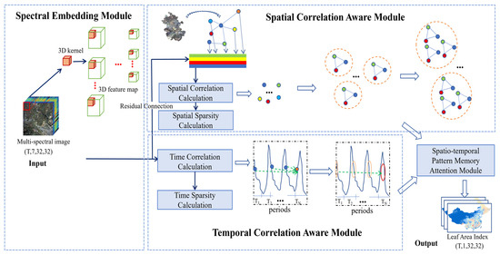
Figure 2.
Network architecture of STC-DeepLAINet.
3.2. Spectral Embedding Module
In LAI inversion, spectral reflectance varies with vegetation coverage, so extracting multidimensional spectral features from remote sensing imagery is crucial for improving inversion accuracy. Due to the complexity of vegetation growth, LAI inversion remote sensing data is typically a 3D data cube, and 3D CNNs can extract these spectral features while enhancing network representational capacity [32]. Thus, we designed a lightweight 3D CNN module. The module comprises four 3D convolutional layers, three pooling layers, and one fully connected layer, each followed by a Rectified Linear Unit (ReLU) activation function. The module input is a sequence of multispectral image cubes denoted as , where each cube represents a spatial patch with 7 spectral bands. The value at position (x,y,z) in the j-th feature map of the i-th convolutional layer is calculated as:
where denotes ReLU, and represent the weights and bias parameter, indexes over the input feature maps from the (i − 1) layer, denotes the input feature value at the corresponding receptive field location., , and represent the height, width, and depth of the 3D convolutional kernel, respectively. Following feature extraction through the 3D CNN, the original input cube is transformed into a high-dimensional temporal feature representation , where N is the number of spatial units, T is the temporal dimension, and d is the final embedding dimension produced by the fully connected layer.
3.3. Spatio-Temporal Correlation Aware Module
3.3.1. Spatial Correlation Aware Module
Considering the inherent spatial autocorrelation of vegetation distribution, we propose a novel spatial embedding method—the spatial location-aware random walk algorithm—which converts graph-based spatial nodes into continuous low-dimensional vector representations to effectively capture spatial neighborhood features [33]. To effectively capture long-range spatial dependencies, a GCN-based spatial correlation aware module (SC) is proposed. Specifically, this method falls into the category of a structured improved graph attention mechanism, thereby enhancing the network’s adaptability to diverse vegetation types.
- (1)
- Capture of similar locations
The correlation between vegetation biophysical properties and geoclimatic conditions underscores the importance of accurately capturing regional geospatial similarities for enhancing LAI inversion accuracy [34]. We utilize a Gaussian kernel to compute the distance between inversion units and , based on their geographic coordinates (latitude and longitude):
where denotes the Euclidean distance between nodes and , and each is defined by its geographic coordinate pair .
Using the calculated spatial distances, the similarity score between node feature vectors and is defined as:
where quantifies the spatial similarity between node and node in the spatial graph . A higher value indicates a stronger similarity between the corresponding geospatial regions.
- (2)
- Spatial location-aware random walk algorithm
We introduce a spatial location-aware random walk strategy based on the above node similarity calculation (Figure 3). For a given node , the algorithm determines the transition to the next node by traversing neighboring nodes based on a non-normalized transition probability , defined as:
where denotes the shortest path distance between node and node . Intuitively, the transition behavior is governed by the similarity score , which adjusts the probability of moving closer to or further from the current node as follows: if , indicating high similarity between two nodes, then , , the traversal path will go from the current node to next node in Figure 3, and the shortest path from to the previous node of the current node is 1, meaning that the walk is more likely to stay near the starting node. If , indicating low similarity, then , , the traversal path will go from the current node to next node or in Figure 3, and the shortest path from or to the previous node of the current node is 2, prompting the walk to explore more distant nodes. When , indicating neutral similarity, the path will backtrack from the current node to the previous node ; therefore, the shortest path is 0. If the shortest distance is greater than 2, needs to jump out of the direct neighborhood of , which violates the core logic of the algorithm that only selects the next step in the neighborhood of the current node. Therefore, only 0, 1, and 2 were selected. This spatial location-aware random walk algorithm integrates both depth-first search and breadth-first search properties, thereby enhancing the balance between local and global sampling, it improves the efficiency and representational quality of node embeddings in the spatial graph.
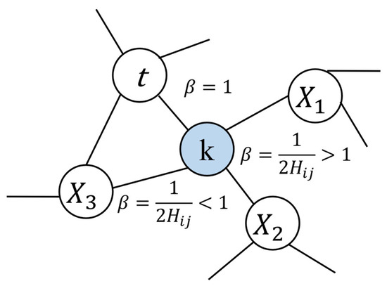
Figure 3.
Illustration of the spatial location-aware random walk algorithm.
- (3)
- Geospatial correlation calculation
A spatial location-aware random walk algorithm is employed to convert geographic location map nodes into low-dimensional embeddings. Then, through the SC (Figure 4), which utilizes geographic location-based correlation calculations, geospatial features associated with the vegetation growth environment are effectively captured. During this learning process, the model can holistically perceive the regional geospatial environment, treating it as continuous geospatial slices rather than isolated pixel-level units, thereby expanding the network’s receptive field.
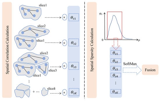
Figure 4.
Illustration of geospatial correlation computation and geospatial sparsity calculation.
The geospatial correlation between slices was computed as follows:
where represents the spatial correlation between a geospatial slice and a subsequent slice separated by offset s. As shown in Figure 4, additional geospatial slices are incrementally added to form an extended spatial region , enabling the network to learn broader spatial dependencies.
- (4)
- Geospatial sparsity calculation
To improve the network computational efficiency, not all geospatial correlation results are fed to subsequent layers. Thus, we designed a sparsity-aware attention mechanism to selectively focus on high-correlation spatial regions. Specifically, spatial slices were first ranked in descending order according to the deviation of their geospatial correlations from a uniform distribution. As shown in Figure 4, the top K spatial slices were selected to construct the final geospatial set denoted as . Let k be a geospatial region augmented with N spatial slices. After projection into query (o), key (p), and value (q) vectors, and given as the dimensionality of each attention subspace:
This ranking strategy identifies the top most relevant spatial slices forming the set . To normalize the attention scores among the selected slices, we apply a SoftMax function:
The attention-weighted spatial correlation output is then computed as:
For the multi-head attention mechanism, with heads, the final output is:
This sparsity-aware attention mechanism helps the network learn spatial dependencies more effectively while reducing excessive computation from less relevant spatial locations.
3.3.2. Temporal Correlation Aware Module
To effectively capture long-term temporal dependencies, the temporal correlation aware module (TC) was designed to capture dependencies not between isolated time points but between aggregated time periods, each composed of multiple temporally adjacent observations; this method is a type of time-series-oriented improved multi-head self-attention, which was based on the fact that vegetation phenology and LAI dynamics are typically governed by continuous growth phases rather than discrete timestamps [35,36]. Its process, analogous to that described in Equations (5) to (9), calculates temporal sparsity to identify the top K most relevant time periods for temporal correlation analysis. Consequently, both temporal correlation computation and temporal sparsity computation were integrated into the TC, enabling the network to learn high-level temporal features from a period-based perspective (Figure 5). This architecture made period-based modeling both biologically and practically meaningful.
Figure 5.
Illustration of temporal correlation computation and temporal sparsity calculation.
3.4. Spatio-Temporal Pattern Memory Attention Module
To dynamically fuse spatio-temporal features and retrieve similar spatio-temporal patterns from historical data, a spatio-temporal pattern memory attention module (MAN) is proposed (Figure 6). This mechanism enabled the model to capture spatio-temporal features from a broader historical context, mitigating the risk of overfitting to localize spatio-temporal patterns [37]; it belongs to the feature-enhanced hybrid gating attention mechanism. Specifically, let and represent the previously learned temporal and spatial features, respectively. The fused spatio-temporal feature was denoted by , and the fusion process was as follows:
where and are learnable parameters, is the bias term, denotes the sigmoid activation function, and Z acts as the gating variable to control the contribution of temporal and spatial features during fusion. This adaptive gating mechanism allows the MAN to dynamically emphasize informative spatio-temporal characteristics learned from historical memory. Within the multi-head attention mechanism, the query vector Q is replaced with the fused spatio-temporal feature , enabling the network to attend more effectively to historically similar spatio-temporal patterns. The output of the MAN was computed as:
where denotes the output of the MAN, denotes the input of the MAN, and represents spatio-temporal memory patterns from previous steps. Finally, the fully connected layer inverted the final LAI values.
Figure 6.
Illustration of spatio-temporal pattern memory attention module.
3.5. Knowledge-Guided Loss Function
To mitigate the saturation effect in LAI inversion that the accuracy significantly decreased when LAI values were greater than 4.0, a knowledge-guided loss function (KLF) that adaptively weights samples based on physiological thresholds was considered in the present study. This function adaptively emphasized samples with higher LAI values by assigning them larger loss weights. In egression tasks, the L2 loss is commonly adopted. Specifically, for a set of training samples , where denotes the input data and represents the corresponding LAI labels, the inverted LAI value is denoted by . Loss function L formally defined as:
where L is the loss function for LAI values > 4.0. The hyperparameter γ is the weighting of the KLF, i.e., when , the penalty on errors for samples with high LAI values is increased considering the supersaturation effects of LAI [38]. This mechanism encourages the network to pay more attention to underrepresented high LAI regions, alleviating the bias introduced by dataset imbalance. Compared to existing saturation correction strategies for high LAI values [39,40,41], the KLF method does not avoid saturation at the data processing stage; rather, it directly regulates the inversion process via the loss function, which exhibits strong generalization ability and can be generalized to different vegetation types.
3.6. Experimental Settings and Evaluation Metrics
All networks were implemented using the PyTorch framework (Version 2.1.0). For STC-DeepLAINet, the base learning rate was set to 1 × 10⁻⁴, with the training process executed for 200 epochs. To ensure experimental fairness, all deep learning models (CNN, Bi-LSTM, AELSTM, GNN-RNN, Transformer, 3D CNN-LSTM) underwent hyperparameter optimization via Bayesian optimization across the following key parameters: learning rate (1 × 10⁻⁴ to 1 × 10⁻²), batch size (16, 32, 64), and dropout rate (0.1–0.5). All deep learning models adopted the Adam optimizer with weight decay of 1 × 10⁻⁵ and early stopping (patience = 20) to prevent overfitting. For traditional machine learning methods (RF, GRNN), hyperparameter tuning was performed via 5-fold cross-validation and grid search as follows: RF was optimized for the number of decision trees (50–500), maximum tree depth (5–30), and minimum samples per leaf (1–10); GRNN was tuned for the spread parameter (σ: 0.01–1.0). All experiments were conducted on a computing platform equipped with an Intel Core i9-13900K CPU (64-bit), an NVIDIA GeForce RTX 4090 GPU, and CUDA Toolkit v12.6.37.
Three quantitative metrics were used to evaluate the performance of the proposed framework, i.e., root mean square error (RMSE), coefficient of determination (R2), and bias. They are defined as follows:
where denotes the number of inverted data points, and represent the labeled and inverted LAI values, respectively, and is the mean of the inverted LAIs.
3.7. Comparison Methods
Eight representative networks including both traditional machine learning and emerging deep learning approaches were employed to evaluate the superiority of the proposed STC-DeepLAINet network.
- (1)
- RF [42]: An ensemble learning method based on decision trees shows robust performance in diverse time-series modeling.
- (2)
- GRNN [43]: Core algorithm of the GLASS V5 LAI product, which estimates LAI by modeling relationships between fused LAI products (MODIS, CYCLOPES) and MODIS surface reflectance.
- (3)
- CNN [44]: A spatial feature extractor for high-dimensional remote sensing imagery also services as a foundational component of our architecture.
- (4)
- Bi-LSTM [45]: It enhances traditional LSTM via forward/backward temporal dependencies, capturing past and future context in sequential data.
- (5)
- AELSTM [46]: Attention-enhanced LSTM, a network that integrates an attention mechanism into LSTM to better capture long-range temporal dependencies for vegetation LAI prediction.
- (6)
- GNN-RNN [47]: Hybrid framework combining Graph Neural Networks (GNNs) for capturing geospatial dependencies and Recurrent Neural Networks (RNNs) for modeling temporal sequences.
- (7)
- Transformer [48]: Deep learning architecture based on self-attention (models long-range dependencies without recurrence) serves as the baseline for the proposed STC-DeepLAINet and was used to produce high-resolution 30m LAI in Jiangsu Province, China.
- (8)
- 3D CNN-LSTM [49]: Hybrid network integrating 3D CNNs and LSTM for spatio-temporal feature extraction from multidimensional satellite imagery.
4. Results
4.1. Exploratory Data Analysis of Fused LAI Training Dataset
To optimize the fused LAI training dataset for STC-DeepLAINet and verify the validity of fusion rules, we compared three fusion strategies (average, median, adaptive) using the ground-based LAI validation dataset as follows: average fusion calculated the arithmetic mean of valid MODIS, VIIRS, and GLASS LAI (GLASS as fallback), median fusion selected the median of the three valid products, and adaptive fusion used the VIIRS-GLASS average (if difference < 1) or the three-product median (GLASS as fallback for invalid MODIS/VIIRS data). Experimental results (Figure 7) showed the adaptive fusion strategy achieved the lowest RMSE (0.56) and highest R2 (0.84), and thus it was adopted to construct the 2019–2020 fused LAI training dataset. Further analysis of the dataset reveals that it covers all major vegetation types in China, including forests, grasslands, croplands, shrublands, and deserts, with forests, grasslands, and croplands as the dominant samples (accounting for 87.1% of the total). This ecologically representative distribution ensured the model’s robust LAI inversion performance across different vegetation types.
Figure 7.
EDA results of the fused LAI training dataset for STC-DeepLAINet. (a) Performance of three LAI fusion strategies (average, median, adaptive); (b) Sample distribution across Chinese vegetation types.
4.2. Comparison with Competing Methods
To evaluate whether STC-DeepLAINet outperformed existing representative networks, comparative experiments were conducted. A comprehensive evaluation of nine methods for LAI inversion at a 500 m spatial resolution across China during 2022–2024 reveals the substantial superiority of our proposed STC-DeepLAINet. According to Table 3, we can find that traditional machine learning methods (RF, GRNN) exhibited the lowest performance, with R2 values below 0.5. In contrast, all deep learning approaches demonstrated better performance, achieving overall R2 values exceeding 0.75. Notably, STC-DeepLAINet showed more gains in performance compared to all reference models, with an average R2 value of 0.96 during 2022–2024, while RMSE and bias were only 0.39 and 0.07, respectively. Moreover, compared with the baseline Transformer, the RMSE of STC-DeepLAINet was reduced by 43%. Overall, our proposed framework consistently outperformed all competing methods across key evaluation metrics including RMSE, R2, and bias.
Table 3.
Performance comparison of different networks for 500 m LAI inversion across China.
Figure 8 presents scatter density plots of the LAI inversion results generated by various deep learning methods compared against the reference fused LAI values (5000 random samples per method). RF and GRNN are excluded from the visualization due to their much lower performance than other methods. The patterns observed in these plots aligned well with the quantitative results presented in Table 3, further validating the superior performance of the proposed STC-DeepLAINet. Among them, the STC-DeepLAINet achieved the highest R2 value of 0.964, which demonstrated its outstanding ability to model complex spatio-temporal correlations inherent in time-series remote sensing imagery. This result highlights the effectiveness of the STC-DeepLAINet in accurately capturing and leveraging spatio-temporal dependencies for LAI inversion.
Figure 8.
Comparison of model-derived across deep learning-based inversion networks versus reference-fused LAI values.
To further analyze the differences in inversion capabilities of various networks, Figure 9 shows the LAI inversion results of different deep learning networks across China in July 2024. Overall, the spatial distribution patterns of LAI generated by these methods were so largely consistent that dense vegetation occurred in northeastern, southeastern, and southwestern China while sparse vegetation was located in northwest China, aligning with known bioclimatic zones [50]. Notably, it is evident that the STC-DeepLAINet produced a more pronounced and detailed distribution across the entire LAI range compared to other methods. Specifically, areas with high LAI values were more clearly delineated in the results obtained using the STC-DeepLAINet, as shown in the red box in Figure 9. This observation highlights the effectiveness of the proposed STC-DeepLAINet in capturing fine-scale spatial variations in vegetation density.
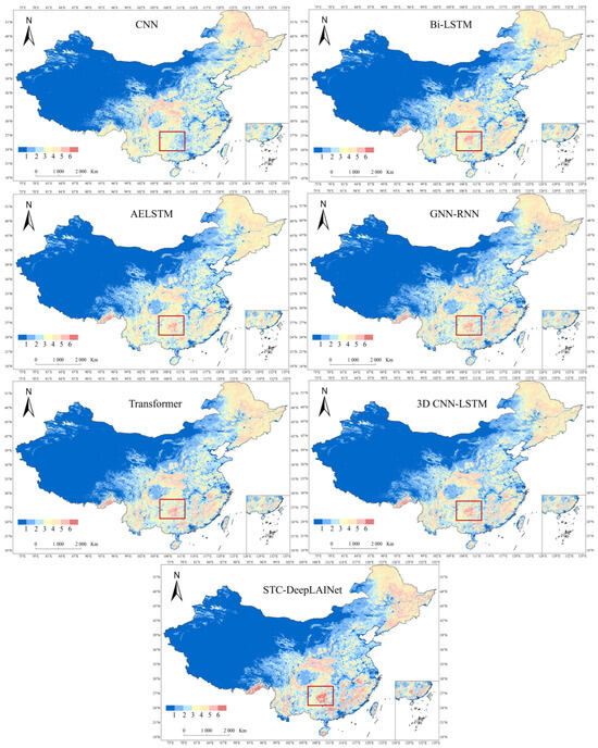
Figure 9.
LAI inversion maps generated by different deep learning networks across China. The red box is used to highlight the differences.
4.3. Module Ablation Study
To verify the effectiveness of each module (i.e., TC, SC, MAN, and KLF) in STC-DeepLAINet, ablation experiments were conducted. As shown in Table 4, TC increased R2 by 4.44–5.81% versus baseline, confirming enhanced temporal feature extraction. Further adding SC to the framework can reduce RMSE by 8.00–18.00%, demonstrating critical spatial context capture. Also, MAN achieved 4.76–8.70% reduction in RMSE through historical pattern inversion. Finally, integrating KLF into the framework reduced the RMSE by 2.56–5.00%, thereby mitigating the saturation effect in LAI inversion. That is, the complete STC-DeepLAINet outperformed all its variants across all metrics, indicating that the combined integration of the TC, SC, MAN, and KLF modules maximized spatio-temporal modeling capability for LAI inversion.
Table 4.
Performance comparison of LAI inversion in China under different strategy configurations. The √ in the rows indicates the included module. The best result is in bold. Arrows show change after module is added: ↓ reduction, ↑ increase.
4.4. Parameter Sensitivity Analysis
To analyze the impact of hyperparameters on model accuracy, the sensitivity of two key hyperparameters K and γ (derived from Equations (6) and (14), respectively) were further analyzed (Figure 10). It can be found that the RMSE of the proposed STC-DeepLAINet exhibited a V-shaped response with initial decreasing before rising, as parameter K varied from 5 to 30 in increments of 5. Optimal inversion performance occurred at K = 25. Both excessively low and high K values reduced performance. This is mainly because a smaller K may capture insufficient contextual information, limiting the network’s ability to model spatial patterns, while a larger K increased computational complexity but introduced more noise, thereby reducing network effectiveness.
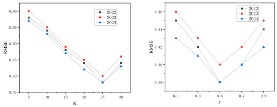
Figure 10.
Impact of hyperparameters K and γ on the LAI inversion accuracy across China.
Adjusting the parameter γ (0.1–0.9, Δ = 0.2) similarly generated a V-shaped curve trend in RMSE with optimal performance at γ = 0.5. Smaller γ caused larger variance for high LAI due to weak knowledge guidance, while larger γ lead to higher bias for high LAI estimates due to insufficient extraction of data features. These experiments demonstrate that precise calibrations of and were crucial for maximizing the performance of STC-DeepLAINet in LAI inversion tasks.
4.5. Validation of LAI Products
To validate the accuracy of the STC-DeepLAINet LAI, comparisons were made with commonly adopted LAI products. When comparing the spatial distribution of LAI inverted by STC-DeepLAINet with that of three widely used LAI products (MODIS, VIIRS, and GLASS) for July 2024 (Figure 11), all four products exhibited similar spatial patterns: higher LAI in southeastern China and lower LAI in northwestern China. Specifically, STC-DeepLAINet yielded higher LAI values than MODIS in agricultural regions, including the Northeast Plain, North China Plain, and Sichuan Basin. Furthermore, in densely forested areas (e.g., the Qinling Mountains and southern Tibet), as shown in the red box in Figure 11, both MODIS and VIIRS LAI showed greater uncertainty and failed to capture the relatively high LAI values observed in GLASS and STC-DeepLAINet products.
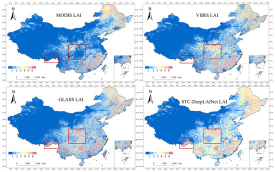
Figure 11.
Spatial distribution of LAI over China from different products for July 2024. The red box is used to highlight the differences.
We further compared the four LAI products across different vegetation types, with results shown in Figure 12. For forests, STC-DeepLAINet exhibited the highest mean and median LAI values among the four products, whereas MODIS showed the lowest. In croplands, STC-DeepLAINet also demonstrated the highest mean and median LAI values, followed by GLASS. However, for the other three vegetation types, differences among the four products were not obvious. These results were consistent with those in Figure 11.
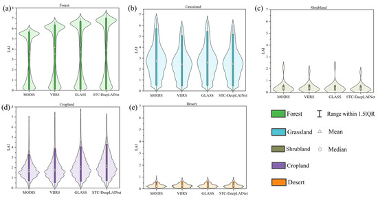
Figure 12.
LAI of the MODIS, VIIRS, GLASS, and STC-DeepLAINet for different land-cover types in July 2024. Data confidence intervals: 5–95%. (a) forest, (b) grassland, (c) shrubland, (d) cropland, (e) desert.
In the validation experiment using ground-based LAI data, ground-based LAI observations are point-scale measurements, while satellite-derived LAI products represent the mean canopy conditions within a 500 m pixel. To reduce the spatial mismatch between these two scales, we employed a widely used scale-matching strategy. For each validation site, the corresponding satellite LAI was extracted as the mean of a 3 × 3 pixel window centered on the site location (covering approximately 1.5 km × 1.5 km). This averaging procedure mitigates the influence of geolocation uncertainty and sub-pixel heterogeneity. Additionally, the coefficient of variation (CV) of LAI within each 3 × 3 neighborhood was calculated to evaluate spatial homogeneity. All sampled neighborhoods exhibited CV values below 0.25, indicating that the surrounding pixels were sufficiently homogeneous for reliable point-to-pixel comparison. In direct validation against ground-based LAI data, STC-DeepLAINet achieved the highest R2 (0.827) and the lowest RMSE (0.718). As illustrated in Figure 13, a greater proportion of STC-DeepLAINet data points fell within the red dashed confidence bounds [51], whereas MODIS data points were more dispersed, indicating superior reliability of STC-DeepLAINet relative to the other three products. Furthermore, STC-DeepLAINet exhibited the strongest correlation with GLASS, yielding an R2 of 0.857 (Figure 14), further supporting the observation in Figure 11 that the spatial distribution of STC-DeepLAINet LAI was most similar to that of GLASS.
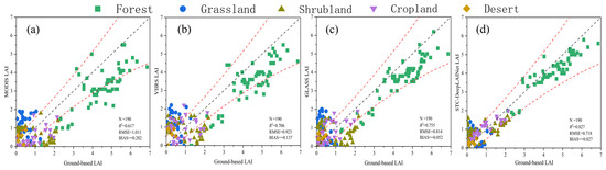
Figure 13.
Direct validation of LAI products using ground-based LAI collected during 2022–2024. (a) MODIS LAI, (b) VIIRS LAI, (c) GLASS LAI, and (d) STC-DeepLAINet LAI. Red dashed lines represent the Global Climate Observing System requires a maximum uncertainty of 15% for the LAI products.
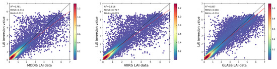
Figure 14.
Scatter density plots comparing STC-DeepLAINet-inverted LAI with other LAI products.
4.6. STC-DeepLAINet’s Tolerance to Cloud/Shadow Noise
To verify the model’s tolerance to typical cloud/shadow noise in LAI inversion, we simulated contamination by setting the 2019–2020 training samples’ reflectance to 0.6 (cloud) or 0.03 (shadow), with three random pixel contamination ratios (10%, 30%, 50%) and noise ratios adjusted from 0 (no distortion) to 1 (complete masking). The RMSE between inverted and ground-measured LAI was used to quantify performance. Experimental results (Figure 15) show that the RMSE of STC-DeepLAINet’s LAI inversion increases with the proportion of contaminated pixels, yet its maximum RMSE is only 0.8—lower than the RMSE values of MODIS LAI (1.01), VIIRS LAI (0.92), and GLASS LAI (0.81) measured under conditions without artificial noise contamination. This indicates that STC-DeepLAINet exhibits strong tolerance to cloud/shadow noise, maintaining superior inversion accuracy even under severe contamination conditions.
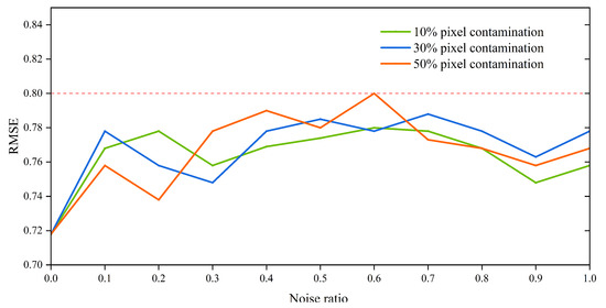
Figure 15.
RMSE of LAI inversion based on training data with 10%, 30%, and 50% pixel contamination ratios. The red dashed line denotes the maximum RMSE of LAI inversion under the simulated noise conditions.
5. Discussion
Comparative experiments demonstrate the superior performance of the proposed STC-DeepLAINet in improving the accuracy of LAI inversion across China, which is primarily attributed to the integration of three key modules (i.e., TC, SC, and MAN). As illustrated in the ablation experiments, RMSE gradually decreased while R2 consistently increased with the sequential addition of these three modules (Table 4). In contrast, traditional machine learning methods (RF, GRNN) exhibited substantially lower R2 values (<0.50) accompanied by larger RMSE (>1.30) and bias (>0.30) (Table 3). Although existing deep learning methods showed certain advantages in LAI inversion with R2 exceeding 0.75, they still failed to fully capture spatio-temporal correlation information. For instance, CNNs are effective in extracting spectral features but neglect temporal continuity [52]. Bi-LSTM networks possess the capability to capture temporal patterns in LAI dynamics (R2 = 0.83) yet perform poorly in modeling spatial correlations [53]. AELSTM network addressed this limitation of Bi-LSTM by incorporating an attention mechanism, reducing RMSE by 12% compared to Bi-LSTM—highlighting the effectiveness of attention mechanisms in emphasizing informative temporal features for LAI inversion [54]. While GNN-RNN and 3D CNN-LSTM can simultaneously capture spatio-temporal and spectral features, they are prone to gradient vanishing or explosion due to their reliance on recurrent structures, thereby restricting their practical effectiveness [55]. In contrast, STC-DeepLAINet, constructed based on the Transformer architecture, overcomes these aforementioned limitations through the three key modules dedicated to spatio-temporal correlation modeling. More importantly, the spatial slices technique and spatial location-aware random walk algorithm were employed to enhance the extraction of spatial correlation information (Table A2). As shown in Table 4, STC-DeepLAINet reduced the average RMSE by 43% compared to the baseline Transformer, demonstrating substantial performance gains derived from its modular design.
Validation using ground-based LAI observations demonstrated that STC-DeepLAINet not only achieved the highest fitting accuracy (surpassing GLASS LAI) but also consistently exhibited the closest alignment with GLASS LAI. This dual outcome further corroborates the reliability of STC-DeepLAINet, as GLASS LAI is widely recognized for its robust consistency with ground-based measurements through previous validation efforts [56,57]. When classified by vegetation type, STC-DeepLAINet retrieved higher LAI values for forests and croplands—an improvement closely related to the introduction of the KLF, which is specifically designed to mitigate the saturation effect commonly encountered in high LAI inversion scenarios (a limitation that plagues the GLASS LAI product). This finding aligns with previous studies that reported the underestimation of LAI (for LAI > 3.0) in northeastern China for GLASS, MODIS, and VIIRS products [58]. Our results further verify this underestimation issue in existing LAI products, particularly for MODIS LAI. As noted in prior research, the lower correlation between MODIS LAI and ground observations may be attributed to the interference of cloudy-sky conditions [8]. In contrast, VIIRS LAI showed a higher correlation due to reduced cloud and atmospheric noise [59], which is consistent with our comparative analysis.
The experimental results of the cloud/shadow noise tolerance test verify that STC-DeepLAINet can maintain stable inversion accuracy even when 50% of training pixels are contaminated, which is of great significance for LAI inversion in cloud-prone regions such as humid agricultural areas. Additionally, the model’s maximum RMSE of 0.8 under noise conditions is lower than the RMSE of existing mainstream LAI products (MODIS LAI: 1.01, VIIRS LAI: 0.92, GLASS LAI: 0.81) without artificial noise contamination, indicating its potential to serve as a reliable alternative to traditional products for more robust time-series LAI monitoring. In addition to this noise tolerance advantage, the model’s universal design (relying on universal spatial-spectral-temporal vegetation features) further broadens its potential for global applicability. The proposed STC-DeepLAINet is not designed for a specific region but relies on universal spatial-spectral-temporal features of vegetation. Furthermore, the MODIS, GLASS, and VIIRS products utilized in this study all provide global coverage. Therefore, STC-DeepLAINet can be applied to geographic regions beyond China. On the other hand, Chen et al. (2025) generated a 30 m spatial resolution, 12-day temporal resolution LAI product for Jiangsu Province (China) in 2023 using multisource remote sensing data—including 500 m MODIS imagery and 30 m Harmonized Landsat and Sentinel-2 (HLS) fused data—via a Transformer deep learning network [48]. When validated against in situ measurements, this product achieved an R2 of 0.62 and an RMSE of 0.79, demonstrating the significant potential of Transformer networks in integrating multi-resolution and multi-sensor data for LAI inversion. Notably, STC-DeepLAINet adopts a Transformer as its backbone network; thus, it holds enormous practical application potential across diverse geographic regions, spatial resolutions, and sensor sources.
The interpretability and reliability challenges posed by the “black box” nature of deep learning networks remain a critical concern in quantitative remote sensing inversion. To address this issue, we innovatively integrated spatio-temporal correlation into the deep learning architecture for LAI inversion and proposed the KLF within STC-DeepLAINet. This dual-design strategy not only effectively mitigated the saturation effect in high LAI inversion but also enhanced the network’s interpretability by embedding physical prior knowledge (i.e., the spatio-temporal continuity of vegetation canopies), thereby significantly improving overall inversion accuracy and reliability. Notably, comprehensive validation against ground-based LAI measurements further confirmed the reliability of the proposed STC-DeepLAINet. Nevertheless, achieving full model transparency remains an ongoing objective. Future research could focus on integrating interpretable deep learning paradigms (e.g., attention visualization, symbolic reasoning) with process-based physical models to develop a knowledge-guided hybrid framework. Such integration is expected to explicitly encode domain knowledge into the network’s learning process, which will not only further enhance the interpretability of inversion results but also promote more credible practical deployment in large-scale remote sensing monitoring of vegetation dynamics.
6. Conclusions
This study proposed STC-DeepLAINet, a Transformer-GCN hybrid deep learning network for large-scale LAI inversion by integrating spatio-temporal correlations. To validate its performance, we conducted a nationwide LAI inversion task at 500 m resolution across China, and the results demonstrate that the framework effectively addresses the existing limitations in extracting complex multidimensional spatio-temporal information from remote sensing imagery. Comparative experiments confirm that STC-DeepLAINet outperforms state-of-the-art deep learning methods and traditional machine learning approaches in three key accuracy metrics (R2, RMSE, and bias). Rigorous ablation studies further clarify the specific contribution of each component to the overall performance. Meanwhile, direct validation against ground-based LAI observations shows that the LAI product derived from STC-DeepLAINet achieves an R2 of 0.827, an RMSE of 0.718, and a bias of −0.027—collectively verifying the high reliability of the proposed framework and its generated product.
These findings have established STC-DeepLAINet as a robust and effective solution for generating large-scale LAI products with integrated spatio-temporal correlations. Theoretically, this work illustrates that the explicit integration of spatio-temporal correlation learning into deep learning architectures provides a promising approach for advancing the inversion of vegetation biophysical parameters. Practically, the framework offers valuable insights for large-scale ecological monitoring, which enhances the capacity to leverage earth observation data for supporting global change research and related decision-making processes.
Author Contributions
Conceptualization, H.W., Q.G. and H.L.; methodology, H.W.; validation, T.T.; investigation, T.T.; data curation, H.W.; writing—original draft preparation, H.W.; writing—review and editing, H.W. and Q.G.; visualization, H.W.; supervision, Q.G. and H.L. All authors have read and agreed to the published version of the manuscript.
Funding
This work was funded by the National Key Research and Development Program of China under Grants 2024YFF1308201.
Data Availability Statement
The original contributions presented in this study are included in the article. Further inquiries can be directed to the corresponding author.
Acknowledgments
The authors thank the National Ecosystem Science Data Center, National Science and Technology Infrastructure of China, and National Tibetan Plateau Data Center for their valuable data support.
Conflicts of Interest
The authors declare no conflicts of interest.
Appendix A
Table A1.
Basic information of ground-based LAI sites used in this study.
Table A1.
Basic information of ground-based LAI sites used in this study.
| Site Name | Year | DOY | Type | Latitude | Longitude |
|---|---|---|---|---|---|
| Heihe River Basin Sidaoqiao Superstation, Inner Mongolia Autonomous Region (http://data.tpdc.ac.cn) | 2022 | 177, 185, 193 | Shrubland | 42.0012 | 101.1374 |
| 2023 | 225, 233, 241, 249, 257, 265, 273, 281, 289, 297 | Shrubland | 42.0012 | 101.1374 | |
| 2024 | 161, 169, 177, 185, 193, 201, 209, 217, 225, 233, 241, 249, 257, 265, 273, 281, 289, 297 | Shrubland | 42.0012 | 101.1374 | |
| Yucheng Station, Shandong (http://www.nesdc.org.cn) | 2022 | 66, 101, 125, 211, 234 | Cropland | 36.8298 | 116.5709 |
| Baotianman Station, Henan (http://www.nesdc.org.cn) | 2023 | 217, 225, 233, 248 | Forest | 33.4997 | 111.9353 |
| Heihe River Basin Daman Superstation, Gansu (http://data.tpdc.ac.cn) | 2022 | 177, 185, 193, 201, 209, 217, 225, 233, 241 | Cropland | 38.8530 | 100.3760 |
| 2024 | 161, 169, 177, 185, 193, 201, 209, 217, 225 | Cropland | 38.8530 | 100.3760 | |
| Qianyanzhou Station, Jiangxi (http://www.nesdc.org.cn) | 2022 | 179, 199, 240, 250, 279 | Forest | 26.7467 | 115.0703 |
| 2023 | 32, 45, 77, 111, 137, 182, 198, 265, 281, 316 | Forest | 26.7467 | 115.0703 | |
| Xishuangbanna Station, Yunnan (http://www.nesdc.org.cn) | 2022 | 26, 57, 85, 116, 146, 177, 207, 238, 269, 299, 330 | Grassland | 21.9269 | 101.2647 |
| 2023 | 26, 57, 85, 116, 146, 177, 207, 238, 269, 299, 330 | Grassland | 21.9269 | 101.2647 | |
| 2024 | 26, 57, 86, 117, 147, 178, 208, 239, 270, 300, 331 | Grassland | 21.9269 | 101.2647 | |
| 2022 | 26, 57, 85, 116, 146, 177, 207, 238, 269, 299, 330 | Shrubland | 21.9233 | 101.2681 | |
| 2023 | 26, 57, 85, 116, 146, 177, 207, 238, 269, 299, 330 | Shrubland | 21.9233 | 101.2681 | |
| 2024 | 26, 57, 86, 117, 147, 178, 208, 239, 270, 300, 331 | Shrubland | 21.9233 | 101.2681 | |
| 2022 | 26, 57, 85, 116, 146, 177, 207, 238, 269 | Forest | 21.9650 | 101.2039 | |
| 2023 | 26, 57, 85, 116, 146, 177, 207, 238, 269 | Forest | 21.9650 | 101.2039 | |
| 2024 | 26, 57, 86, 117, 147, 178, 208, 239, 270, 300, 331 | Forest | 21.9650 | 101.2039 | |
| Dunhuang, Gansu (LAI-2200) | 2022 | 257, 265, 273, 281, 289 | Desert | 39.4912 | 94.2706 |
| Qingyuan, Liaoning (LAI-2200) | 2022 | 185, 193, 201, 209 | Forest | 41.8333 | 124.9167 |
| Hulunbuir, Inner Mongolia Autonomous Region (LAI-2200) | 2023 | 225, 233, 241 | Grassland | 49.2113 | 120.0681 |
| Langfang, Hebei (LAI-2200) | 2022 | 225, 233, 241 | Cropland | 39.1333 | 115.8000 |
| Mianyang, Sichuan (LAI-2200) | 2024 | 185, 193, 201 | Cropland | 31.2667 | 105.4500 |
| Nyingchi, Tibet Autonomous Region (LAI-2200) | 2023 | 193, 201, 209, 217 | Forest | 29.6500 | 94.7833 |
Table A2.
A comparison of LAI inversion performance in China: With vs. without the spatial location-aware random walk algorithm. The √ in the rows indicates the included module. Arrows show change after module is added: ↓ reduction, ↑ increase.
Table A2.
A comparison of LAI inversion performance in China: With vs. without the spatial location-aware random walk algorithm. The √ in the rows indicates the included module. Arrows show change after module is added: ↓ reduction, ↑ increase.
| Year | Strategy | ||||
|---|---|---|---|---|---|
| SC with No SLRW | SC with SLRW | RMSE | R2 | Bias | |
| 2022 | √ | 0.45 | 0.93 | 0.10 | |
| √ | 0.41 ↓ 8.89% | 0.94 ↑ 1.08% | 0.08 ↓ 20.00% | ||
| 2023 | √ | 0.48 | 0.93 | 0.09 | |
| √ | 0.46 ↓ 4.17% | 0.94 ↑ 1.08% | 0.08 ↓ 11.11% | ||
| 2024 | √ | 0.44 | 0.94 | 0.10 | |
| √ | 0.42 ↓ 4.55% | 0.95 ↑ 1.06% | 0.09 ↓ 10.00% | ||
References
- Qi, J.; Xie, D.; Jiang, J.; Huang, H. 3D radiative transfer modeling of structurally complex forest canopies through a lightweight boundary-based description of leaf clusters. Remote Sens. Environ. 2022, 283, 113301. [Google Scholar] [CrossRef]
- Yan, K.; Gao, S.; Yan, G.; Ma, X.; Chen, X.; Zhu, P.; Li, J.; Gao, S.; Gastellu-Etchegorry, J.-P.; Myneni, R.B.; et al. A global systematic review of the remote sensing vegetation indices. Int. J. Appl. Earth Obs. Geoinf. 2025, 139, 104560. [Google Scholar] [CrossRef]
- Sun, Y.; Qin, Q.; Zhang, Y.; Ren, H.; Han, G.; Zhang, Z.; Zhang, T.; Wang, B. A leaf chlorophyll vegetation index with reduced LAI effect based on Sentinel-2 multispectral red-edge information. Comput. Electron. Agric. 2025, 236, 110500. [Google Scholar] [CrossRef]
- Xu, J.; Du, X.; Dong, T.; Li, Q.; Zhang, Y.; Wang, H.; Liu, M.; Zhu, J.; Yang, J. Estimation of sugarcane biomass from Sentinel-2 leaf area index using an improved SAFY model (SAFY-Sugar). Int. J. Appl. Earth Obs. Geoinf. 2025, 140, 104570. [Google Scholar] [CrossRef]
- IPCC. Climate Change 2022: Impacts, Adaptation and Vulnerability; Summary for Policymakers; IPCC: Geneva, Switzerland, 2022. [Google Scholar]
- Zhang, S.; Korhonen, L.; Lang, M.; Pisek, J.; Diaz, G.M.; Korpela, I.; Xia, Z.; Haapala, H.; Maltamo, M. Comparison of semi-physical and empirical models in the estimation of boreal forest leaf area index and clumping with airborne laser scanning data. IEEE Trans. Geosci. Remote Sens. 2024, 62, 5701212. [Google Scholar] [CrossRef]
- Zhang, X.; Yan, K.; Liu, J.; Yang, K.; Pu, J.; Yan, G.; Heiskanen, J.; Zhu, P.; Knyazikhin, Y.; Myneni, R.B. An Insight into the Internal Consistency of MODIS Global Leaf Area Index Products. IEEE Trans. Geosci. Remote Sens. 2024, 62, 4411716. [Google Scholar] [CrossRef]
- Ma, H.; Liang, S. Development of the GLASS 250-m leaf area index product (version 6) from MODIS data using the bidirectional LSTM deep learning model. Remote Sens. Environ. 2022, 273, 112985. [Google Scholar] [CrossRef]
- Démoulin, R.; Gastellu-Etchegorry, J.P.; Lefebvre, S.; Briottet, X.; Zhen, Z.; Adeline, K.; Marionneau, M.; Le Dantec, V. Modeling 3D radiative transfer for maize traits retrieval: A growth stage-dependent study on hyperspectral sensitivity to field geometry, soil moisture, and leaf biochemistry. Remote Sens. Environ. 2025, 327, 114784. [Google Scholar] [CrossRef]
- Kallel, A.; Wang, Y.; Hedman, J.; Gastellu-Etchegorry, J.P. Canopy BRDF differentiation on LAI based on Monte Carlo Ray Tracing. Remote Sens. Environ. 2025, 327, 114785. [Google Scholar] [CrossRef]
- Sun, Y.; Qin, Q.; Ren, H.; Zhang, T.; Chen, S. Red-edge band vegetation indices for leaf area index estimation from Sentinel-2/MSI imagery. IEEE Trans. Geosci. Remote Sens. 2020, 58, 826–840. [Google Scholar] [CrossRef]
- Myneni, R.B.; Hoffman, S.; Knyazikhin, Y.; Privette, J.L.; Glassy, J.; Tian, Y.; Wang, Y.; Song, X.; Zhang, Y.; Smith, G.R.; et al. Global products of vegetation leaf area and fraction absorbed PAR from year one of MODIS data. Remote Sens. Environ. 2002, 83, 214–231. [Google Scholar] [CrossRef]
- Yang, Y.; Huang, Q.; Wu, Z.; Wu, T.; Luo, J.; Dong, W.; Sun, Y.; Zhang, X.; Zhang, D. Mapping crop leaf area index at the parcel level via inverting a radiative transfer model under spatiotemporal constraints: A case study on sugarcane. Comput. Electron. Agric. 2022, 198, 107003. [Google Scholar] [CrossRef]
- Sun, L.; Wang, W.; Jia, C.; Liu, X. Leaf area index remote sensing based on Deep Belief Network supported by simulation data. Int. J. Remote Sens. 2021, 42, 7637–7661. [Google Scholar] [CrossRef]
- Zhang, Y.; Gao, J.; Zhang, D.; Liang, T.; Wang, Z.; Zhang, X.; Ma, Z.; Yang, J. Improved estimation of forage nitrogen in alpine grassland by integrating Sentinel-2 and SIF data. Plant Methods 2025, 21, 69. [Google Scholar] [CrossRef]
- Ge, X.; Yang, Y.; Peng, L.; Chen, L.; Li, W.; Zhang, W.; Chen, J. Spatio-Temporal Knowledge Graph Based Forest Fire Prediction with Multi Source Heterogeneous Data. Remote Sens. 2022, 14, 3496. [Google Scholar] [CrossRef]
- Jin, D.; Qi, J.; Huang, H.; Li, L. Combining 3D radiative transfer model and convolutional neural network to accurately estimate forest canopy cover from very high-resolution satellite images. IEEE J. Sel. Top. Appl. Earth Obs. Remote Sens. 2021, 14, 10953–10963. [Google Scholar] [CrossRef]
- Liu, T.; Jin, H.; Xie, X.; Fang, H.; Wei, D.; Li, A. Bi-LSTM model for time series leaf area index estimation using multiple satellite products. IEEE Geosci. Remote Sens. Lett. 2022, 19, 1–5. [Google Scholar] [CrossRef]
- Song, R.; Feng, Y.; Cheng, W.; Mu, Z.; Wang, X. BS2T: Bottleneck Spatial-Spectral Transformer for Hyperspectral Image Classification. IEEE Trans. Geosci. Remote Sens. 2022, 60, 1–17. [Google Scholar] [CrossRef]
- Zou, Y.; Wang, J.; Lei, P.; Li, Y. A novel multi-step ahead forecasting model for flood based on time residual LSTM. J. Hydrol. 2023, 620, 129521. [Google Scholar] [CrossRef]
- Vaswani, A.; Shazeer, N.; Parmar, N.; Uszkoreit, J.; Jones, L.; Gomez, A.N.; Kaiser, L.; Polosukhin, I. Attention is all you need. In Proceedings of the 31st Annual Conference on Neural Information Processing Systems, Long Beach, CA, USA, 4 December 2017. [Google Scholar]
- Chen, P.; Zhang, Y.; Cheng, Y.; Shu, Y.; Wang, Y.; Wen, Q.; Yang, B.; Guo, C. Pathformer: Multi-scale transformers with adaptive pathways for time series forecasting. In Proceedings of the 12th The International Conference on Learning Representations, Vienna, Austria, 7 May 2024. [Google Scholar]
- Wang, Y.; Jing, C.; Xu, S.; Guo, T. Attention based spatiotemporal graph attention networks for traffic flow forecasting. Inf. Sci. 2022, 607, 869–883. [Google Scholar] [CrossRef]
- Li, X.; Sun, L.; Ling, M.; Peng, Y. A survey of graph neural network based recommendation in social networks. Neurocomputing 2023, 549, 126441. [Google Scholar] [CrossRef]
- Sun, Y.; Deng, K.; Ren, K.; Liu, J.; Deng, C.; Jin, Y. Deep learning in statistical downscaling for deriving high spatial resolution gridded meteorological data: A systematic review. ISPRS J. Photogramm. Remote Sens. 2024, 208, 14–38. [Google Scholar] [CrossRef]
- Friedl, M.; Sulla-Menashe, D. MODIS/Terra+Aqua Land Cover Type Yearly L3 Global 500m SIN Grid V061. NASA Land Process. Distrib. Act. Arch. Cent. 2022. Available online: https://www.earthdata.nasa.gov/data/catalog/lpcloud-mcd12q1-061 (accessed on 10 December 2025).
- Myneni, R. VIIRS/NPP Leaf Area Index/FPAR 8-Day L4 Global 500m SIN Grid V002 [Data set]. NASA Land Process. Distrib. Act. Arch. Cent. 2022. [Google Scholar] [CrossRef]
- Vermote, E.F.; Ray, J.P. MODIS Surface Reflectance User’s Guide Collection [User Guide/Technical Report]; NASA Land Processes Distributed Active Archive Center (LP DAAC): Sioux Falls, SD, USA, 2015; pp. 1–37. Available online: https://www.earthdata.nasa.gov/data/catalog/lpcloud-mod09a1-061 (accessed on 10 December 2025).
- Liu, S.; Xu, Z.; Che, T.; Li, X.; Xu, T.; Ren, Z.; Zhang, Y.; Tan, J.; Song, L.; Zhou, J.; et al. A dataset of energy, water vapor, and carbon exchange observations in oasis-desert areas from 2012 to 2021 in a typical endorheic basin. Earth Syst. Sci. Data 2023, 15, 4959–4981. [Google Scholar] [CrossRef]
- Pu, J.; Yan, K.; Gao, S.; Zhang, Y.; Park, T.; Sun, X.; Weiss, M.; Knyazikhin, Y.; Myneni, R.B. Improving the MODIS LAI compositing using prior time-series information. Remote Sens. Environ. 2023, 287, 113493. [Google Scholar] [CrossRef]
- Román, M.O.; Justice, C.; Paynter, I.; Boucher, P.B.; Devadiga, S.; Endsley, A.; Erb, A.; Friedl, M.; Gao, H.; Giglio, L.; et al. Continuity between NASA MODIS Collection 6.1 and VIIRS Collection 2 land products. Remote Sens. Environ. 2024, 302, 113963. [Google Scholar] [CrossRef]
- Roy, S.K.; Krishna, G.; Dubey, S.R.; Chaudhuri, B.B. HybridSN: Exploring 3-D-2-D CNN feature hierarchy for hyperspectral image classification. IEEE Geosci. Remote Sens. Lett. 2020, 17, 277–281. [Google Scholar] [CrossRef]
- Zoubir, A.; Missaoui, B. Graph Neural Networks with scattering transform for network anomaly detection. Eng. Appl. Artif. Intell. 2025, 150, 110546. [Google Scholar] [CrossRef]
- Zhang, Y.; Han, X.; Yang, J. Estimation of leaf area index over heterogeneous regions using the vegetation type information and PROSAIL model. IEEE J. Sel. Top. Appl. Earth Obs. Remote Sens. 2023, 16, 5405–5415. [Google Scholar] [CrossRef]
- Caparros-Santiago, J.A.; Rodriguez-Galiano, V.; Dash, J. Land surface phenology as indicator of global terrestrial ecosystem dynamics: A systematic review. ISPRS J. Photogramm. Remote Sens. 2021, 171, 330–347. [Google Scholar] [CrossRef]
- Wu, H.; Xu, J.; Wang, J.; Long, M. Autoformer: Decomposition transformers with auto-correlation for long-term series forecasting. In Proceedings of the 35th Conference on Neural Information Processing Systems, Online, 6–14 December 2021. [Google Scholar]
- Liu, A.; Zhang, Y. An efficient spatial-temporal transformer with temporal aggregation and spatial memory for traffic forecasting. Expert Syst. Appl. 2024, 250, 123884. [Google Scholar] [CrossRef]
- Xu, D.D.; An, D.S.; Guo, X.L. The Impact of Non-Photosynthetic Vegetation on LAI Estimation by NDVI in Mixed Grassland. Remote Sens. 2020, 12, 1979. [Google Scholar] [CrossRef]
- Zhang, H.; Wang, G.; Song, F.; Wen, Z.; Li, W.; Tong, L.; Kang, S. Improving chili pepper LAI prediction with TPE-2BVIs and UAV hyperspectral imagery. Comput. Electron. Agric. 2025, 235, 110368. [Google Scholar] [CrossRef]
- Li, H.; Li, P.; Xu, X.; Feng, H.; Xu, B.; Long, H.; Yang, G.; Zhao, C. Revealing the spectral bands that make generic remote estimates of leaf area index in wheat crop over various interference factors and planting conditions. Comput. Electron. Agric. 2025, 235, 110381. [Google Scholar] [CrossRef]
- Mulero, G.; Bonfil, D.J.; Helman, D. Wheat leaf area index retrieval from drone-derived hyperspectral and LiDAR imagery using machine learning algorithms. Agric. For. Meteorol. 2025, 372, 110648. [Google Scholar] [CrossRef]
- Gao, X.; Yao, Y.; Chen, S.; Li, Q.; Zhang, X.; Liu, Z.; Zeng, Y.; Ma, Y.; Zhao, Y.; Li, S. Improved maize leaf area index inversion combining plant height corrected resampling size and random forest model using UAV images at fine scale. Eur. J. Agron. 2024, 161, 127360. [Google Scholar] [CrossRef]
- Xiao, Z.; Liang, S.; Wang, J.; Chen, P.; Yin, X.; Zhang, L.; Song, J. Use of general regression neural networks for generating the GLASS leaf area index product from time-series MODIS surface reflectance. IEEE Trans. Geosci. Remote Sens. 2014, 52, 209–223. [Google Scholar] [CrossRef]
- Ilniyaz, O.; Du, Q.; Shen, H.; He, W.; Feng, L.; Azadi, H.; Kurban, A.; Chen, X. Leaf area index estimation of pergola-trained vineyards in arid regions using classical and deep learning methods based on UAV-based RGB images. Comput. Electron. Agric. 2023, 207, 107723. [Google Scholar] [CrossRef]
- Zhou, J.; Yang, Q.; Liu, L.; Kang, Y.; Jia, X.; Chen, M.; Ghosh, R.; Xu, S.; Jiang, C.; Guan, K.; et al. A deep transfer learning framework for mapping high spatiotemporal resolution LAI. ISPRS J. Photogramm. Remote Sens. 2023, 206, 30–48. [Google Scholar] [CrossRef]
- Xiong, Z.; Zhang, Z.; Gui, H.; Zhu, P.; Sun, Y.; Zhou, X.; Xiao, K.; Xin, Q. Predicting time series of vegetation leaf area index across North America based on climate variables for land surface modeling using attention-enhanced LSTM. Int. J. Digit. Earth. 2024, 17, 2372317. [Google Scholar] [CrossRef]
- Fan, J.; Bai, J.; Li, Z.; Ortiz-Bobea, A.; Gomes, C.P.; Assoc Advancement Artificial, I. A GNN-RNN approach for harnessing geospatial and temporal information: Application to crop yield prediction. In Proceedings of the 36th AAAI Conference on Artificial Intelligence, Philadelphia, PA, USA, 22 February–1 March 2022. [Google Scholar]
- Chen, P.; Zhou, K.; Fang, H. High-Resolution Seamless Mapping of the Leaf Area Index via Multisource Data and the Transformer Deep Learning Model. IEEE Trans. Geosci. Remote Sens. 2025, 63, 4408512. [Google Scholar] [CrossRef]
- Qiao, M.; He, X.; Cheng, X.; Li, P.; Luo, H.; Zhang, L.; Tian, Z. Crop yield prediction from multi-spectral, multi-temporal remotely sensed imagery using recurrent 3D convolutional neural networks. Int. J. Appl. Earth Obs. Geoinf. 2021, 102, 102436. [Google Scholar] [CrossRef]
- Zhang, X.; Wang, Z.; Hou, F.; Yang, J.; Guo, X. Terrain evolution of China seas and land since the Indo-China movement and characteristics of the stepped landform. Chin. J. Geophys-Ch. 2014, 57, 3968–3980. [Google Scholar] [CrossRef]
- Fang, H.; Baret, F.; Plummer, S.; Schaepman-Strub, G. An Overview of Global Leaf Area Index (LAI): Methods, Products, Validation, and Applications. Rev. Geophys. 2019, 57, 739–799. [Google Scholar] [CrossRef]
- Bazgir, O.; Zhang, R.; Dhruba, S.R.; Rahman, R.; Ghosh, S.; Pal, R. Representation of features as images with neighborhood dependencies for compatibility with convolutional neural networks. Nat. Commun. 2020, 11, 4391. [Google Scholar] [CrossRef]
- Du, S.; Li, T.; Yang, Y.; Horng, S.J. Deep Air Quality Forecasting Using Hybrid Deep Learning Framework. IEEE Trans. Knowl. Data Eng. 2021, 33, 2412–2424. [Google Scholar] [CrossRef]
- Zhang, X.; Guo, Y.; Shangguan, H.; Li, R.; Wu, X.; Wang, A. Predicting remaining useful life of a machine based on embedded attention parallel networks. Mech. Syst. Signal Process. 2023, 192, 110221. [Google Scholar] [CrossRef]
- Sun, P.; Wu, J.; Zhang, M.; Devos, P.; Botteldooren, D. Delayed Memory Unit: Modeling Temporal Dependency Through Delay Gate. IEEE Trans. Neural Netw. Learn. Syst. 2025, 36, 10808–10818. [Google Scholar] [CrossRef]
- Li, X.; Lu, H.; Yu, L.; Yang, K. Comparison of the spatial characteristics of four remotely sensed leaf area index products over China: Direct validation and relative uncertainties. Remote Sens. 2018, 10, 148. [Google Scholar] [CrossRef]
- Zheng, J.M.; Wang, M.Y.; Liang, M.Y.; Gao, Y.Y.; Tan, M.L.; Liu, M.Y.; Wang, X.P. Influence of terrain on MODIS and GLASS leaf area index (LAI) products in Qinling Mountains forests. Forests 2024, 15, 1871. [Google Scholar] [CrossRef]
- Fang, H.L.; Zhang, Y.H.; Wei, S.S.; Li, W.J.; Ye, Y.C.; Sun, T.; Liu, W.W. Validation of global moderate resolution leaf area index (LAI) products over croplands in northeastern China. Remote Sens. Environ. 2019, 233, 111377. [Google Scholar] [CrossRef]
- Yan, K.; Pu, J.; Park, T.; Xu, B.; Zeng, Y.; Yan, G.; Weiss, M.; Knyazikhin, Y.; Myneni, R.B. Performance stability of the MODIS and VIIRS LAI algorithms inferred from analysis of long time series of products. Remote Sens. Environ. 2021, 260, 112438. [Google Scholar] [CrossRef]


Disclaimer/Publisher’s Note: The statements, opinions and data contained in all publications are solely those of the individual author(s) and contributor(s) and not of MDPI and/or the editor(s). MDPI and/or the editor(s) disclaim responsibility for any injury to people or property resulting from any ideas, methods, instructions or products referred to in the content. |
© 2025 by the authors. Licensee MDPI, Basel, Switzerland. This article is an open access article distributed under the terms and conditions of the Creative Commons Attribution (CC BY) license (https://creativecommons.org/licenses/by/4.0/).