Validation of the CERES Clear-Sky Surface Longwave Downward Radiation Products Under Air Temperature Inversion

Highlights

What are the main findings?

• The accuracy of CERES SLDR products is degraded heavily under ATI conditions.
• The concurrent atmospheric moisture inversion (AMI) compounds this degradation.
• It is urgent to refine CERES SLDR algorithms in the future.

What are the implications of the main findings?

• Advance our understanding of the clear-sky SLDR estimate mechanism.
• Provide valuable guidance and benefit the CERES SLDR product users.

Abstract

This study assessed the performance of the Clouds and the Earth’s Radiant Energy System (CERES) surface longwave downward radiation (SLDR) products under the atmospheric temperature inversion (ATI) conditions for the first time. Three years of ground-measured SLDRs from 409 globally distributed stations across four flux networks were employed, and the collocated MODIS atmospheric profile product was used to identify the ATI profiles at each flux station. All three SLDR estimate algorithms (Models A, B, and C) show a pronounced accuracy decline under ATI conditions, regardless of region (polar or non-polar) or time of day (daytime or nighttime). Under ATI conditions, the Bias/RMSE increases by approximately 10.0/5.0 W/m² for Models A and B, 5.0/1.0 W/m² for Model C. Sensitivity analysis reveals that the concurrent atmospheric moisture inversion (AMI) compounds this degradation; both the Bias and RMSE increase with the AMI intensity. These results underscore the need to refine CERES SLDR algorithms in the future.

1. Introduction

Surface longwave (LW) downward radiation (SLDR) is a crucial component of the surface radiation balance [1,2,3]. SLDR reflects the radiation exchange between the atmosphere and the surface, typically regulated by factors such as atmospheric temperature, water vapor, aerosols, and cloud cover [4,5]. An accurate estimate of SLDR has become one of the core tasks in climate and environmental research. Remote sensing has been acknowledged as a unique and effective means to map SLDR globally at a finer scale. A couple of typical global SLDR products have been released over the past three decades; for example, coarse-resolution (~1°) products like the Global Energy and Water Cycle Experiment–Surface Radiation Budget (GEWEX-SRB) [6], the International Satellite Cloud Climatology Project–Flux Data (ISCCP-FD) [7], and the Clouds and the Earth’s Radiant Energy System–Gridded Radiative Fluxes and Clouds (CERES-FSW) [8,9,10]; and the fine-resolution (1 km) Essential thermaL Infrared remoTe sEnsing (ELITE) SLDR product [11]. These SLDR products have benefited scientists in the field of climate change.

Air temperature inversion (ATI) is a common weather phenomenon that usually occurs at the near-surface boundary layer, especially in mountainous regions and the Antarctic Plateau [12]. The occurrence of the ATI alters the atmospheric state at the near-surface boundary layer and affects the accuracy of the clear-sky SLDR estimate, but is ignored in the production of the typical satellite SLDR products mentioned above. Dupont et al. [13] proposed a new parametric model for predicting the clear-sky SLDR by considering the variations in vertical distribution of water vapor (the ratio of screen-level to column-integrated water vapor density) and variations in the temperature lapse rate (the ratio of screen-level temperature to the minimum temperature during the day) based on an analysis of the parameterization schemes developed by Brutsaert [14] and Prata [15]. Yu et al. [16] developed a parameterization scheme that estimates the clear-sky SLDR using MODIS brightness temperature and integrated water vapor. The scheme can improve the SLDR estimate accuracy under high water vapor content and is claimed to be insensitive to temperature inversion. Cheng et al. [17] revealed the mechanism by which the ATI affects the estimate accuracy of SLDR and developed a correction method that substantially improves the accuracy of six typical parameterization schemes when validated at SURFRAD sites.

Despite these advances, critical issues in the SLDR estimate under ATI remain unresolved and require further exploration. One major unresolved issue is the lack of comprehensive validation of global satellite-based SLDR products under ATI conditions, including CERES SLDR products. Thus, this study evaluates the performance of the current SLDR estimate algorithm under ATI conditions, using the widely adopted CERES SLDR product algorithms as an example. The paper is structured as follows: Section 2 describes the ground measurements, satellite datasets and evaluation method; Section 3 presents the validation results; Section 4 is the Discussion, and Section 5 summarizes the main conclusions.

2. Materials and Methods

2.1. CERES-SSF SLDR Product

CERES is a National Aeronautics and Space Administration (NASA) satellite project that studies the role of clouds, aerosols, and radiation in the Earth’s climate system [10]. Each file of the Single Scanner Footprint top-of-atmosphere (TOA)/Surface Fluxes and Clouds (SSF) product contains one hour of instantaneous CERES data for a single scanner footprint (~20 km) from Terra and Aqua spacecraft observations. It combines CERES data with scene information from MODIS data on cloud and aerosol properties to derive instantaneous, all-sky SLDR. The CERES-SSF Edition 4A product was employed in this study.

The product provides three SLDR datasets derived from LW Models A, B, and C, suitable for different climatic conditions and radiative scenarios. As reported by Kratz et al. [9], the CERES LW Models for SLDR show global biases below 10 W/m² and RMSEs below 26 W/m² for clear-sky conditions, with larger biases in deserts (10–20 W/m²) and polar regions (~30 W/m²). Under cloudy-sky conditions, biases remain small (<6 W/m²), but RMSEs are substantially higher (20–30 W/m²), particularly in polar regions (up to 26.7–28.6 W/m²).

2.1.1. Model A

This algorithm was developed by Inamdar and Ramanathan [18], which calculates SLDR as the sum of the window and non-window components.

$$\mathrm{S}\mathrm{L}\mathrm{D}\mathrm{R}={\mathrm{F}}_{\mathrm{d},\mathrm{w}\mathrm{i}\mathrm{n}}+{\mathrm{F}}_{\mathrm{d},\mathrm{n}\mathrm{w}}$$

(1)

where ${\mathrm{F}}_{\mathrm{d},\mathrm{w}\mathrm{i}\mathrm{n}}$ and ${\mathrm{F}}_{\mathrm{d},\mathrm{n}\mathrm{w}}$ represent the window and non-window $\mathrm{S}\mathrm{L}\mathrm{D}\mathrm{R}$, respectively. The physics of radiative transfer in the window and non-window spectral regions form the basis of this algorithm; the TOA and surface longwave radiations are simulated using a broadband radiative transfer model, which uses soundings from ship sondes as input.

The atmospheric greenhouse effect (${\mathrm{G}}_{\mathrm{a}}$) is the key radiometric quantity in the parameterization since there is a close affinity between ${\mathrm{G}}_{\mathrm{a}}$ and $\mathrm{S}\mathrm{L}\mathrm{D}\mathrm{R}$.

$${\mathrm{G}}_{\mathrm{a}}={\displaystyle \underset{{\mathrm{z}}_{\mathrm{t}\mathrm{o}\mathrm{p}}}{\overset{0}{\int }}\mathrm{A}({\mathrm{z}}_{\mathrm{t}\mathrm{o}\mathrm{p}},{\mathrm{z}}^{\prime })\frac{\mathrm{d}\mathrm{B}({\mathrm{z}}^{\prime })}{\mathrm{d}{\mathrm{z}}^{\prime }}}\mathrm{d}{\mathrm{z}}^{\prime }$$

(2)

where $\mathrm{B}({\mathrm{z}}^{\prime })$ is the Planck function, $\mathrm{A}(\mathrm{z},{\mathrm{z}}^{\prime })$ is the atmospheric absorptance between the levels specified in the arguments, and ${\mathrm{z}}_{\mathrm{t}\mathrm{o}\mathrm{p}}$ is the altitude at the top of the atmosphere. Ramanathan [19] then described the greenhouse effect in terms of the difference

$${\mathrm{G}}_{\mathrm{a}}={\mathrm{F}}_{\mathrm{L}\mathrm{W}}^{\uparrow }(\mathrm{S}\mathrm{F}\mathrm{C})-{\mathrm{F}}_{\mathrm{L}\mathrm{W}}^{\uparrow }(\mathrm{T}\mathrm{O}\mathrm{A})$$

(3)

where ${\mathrm{F}}_{\mathrm{L}\mathrm{W}}^{\uparrow }(\mathrm{S}\mathrm{F}\mathrm{C})$ is the surface longwave upward radiation (SLUR), and ${\mathrm{F}}_{\mathrm{L}\mathrm{W}}^{\uparrow }(\mathrm{T}\mathrm{O}\mathrm{A})$ is the window upward longwave TOA radiation.

The model A explained the SLDR in the window and non-window region in terms of their respective components of ${\mathrm{G}}_{\mathrm{a}}$ and other residual variables:

$${\mathrm{F}}_{\mathrm{d},\mathrm{w}\mathrm{i}\mathrm{n}}-{\mathrm{a}}_0{\mathrm{g}}_{\mathrm{a},\mathrm{w}\mathrm{i}\mathrm{n}}={\mathrm{c}}_0+{\mathrm{F}}_{\mathrm{t}\mathrm{o}\mathrm{a},\mathrm{w}\mathrm{i}\mathrm{n}}{\displaystyle \sum _{\mathrm{i}}{\mathrm{c}}_{\mathrm{i}}{\mathrm{P}}_{\mathrm{i}}}$$

(4)

$${\mathrm{F}}_{\mathrm{d},\mathrm{n}\mathrm{w}}-{\mathrm{b}}_0{\mathrm{g}}_{\mathrm{a},\mathrm{n}\mathrm{w}}={\mathrm{d}}_0+{\mathrm{F}}_{\mathrm{t}\mathrm{o}\mathrm{a},\mathrm{n}\mathrm{w}}{\displaystyle \sum _{\mathrm{i}}{\mathrm{d}}_{\mathrm{i}}{\mathrm{P}}_{\mathrm{i}}}$$

(5)

where ${\mathrm{F}}_{\mathrm{d},\mathrm{w}\mathrm{i}\mathrm{n}}$ and ${\mathrm{F}}_{\mathrm{d},\mathrm{n}\mathrm{w}}$ are the window and non-window SLDR, respectively. ${\mathrm{g}}_{\mathrm{a},\mathrm{w}\mathrm{i}\mathrm{n}}$ and ${\mathrm{g}}_{\mathrm{a},\mathrm{n}\mathrm{w}}$ represent the window and non-window components of the greenhouse effect. ${\mathrm{F}}_{\mathrm{t}\mathrm{o}\mathrm{a},\mathrm{w}\mathrm{i}\mathrm{n}}$ and ${\mathrm{F}}_{\mathrm{t}\mathrm{o}\mathrm{a},\mathrm{n}\mathrm{w}}$ are the window and non-window upward longwave TOA radiation, respectively. ${\mathrm{P}}_{\mathrm{i}}$ is a combination of parameters such as the window (or non-window) SLUR, the total column water vapor ($\mathrm{w}$), the air temperature in the vicinity of the surface (${\mathrm{\theta }}_{\mathrm{a}}$), and the surface air temperature (${\mathrm{\theta }}_0$). ${\mathrm{a}}_0$, ${\mathrm{b}}_0$, ${\mathrm{c}}_{\mathrm{i}}$, and ${\mathrm{d}}_{\mathrm{i}}$ are regression coefficients which vary with the geographic region.

2.1.2. Model B

Model B builds upon the Langley Parameterized Longwave Algorithm (LPLA), developed from an accurate narrowband radiative transfer model [5]. The clear-sky SLDR is represented in terms of the water vapor and temperature distribution close to the surface according to extensive sensitivity tests:

$${\mathrm{SLDR}}_{\mathrm{d},\mathrm{c}}=({\mathrm{A}}_0+{\mathrm{A}}_1\mathrm{V}+{\mathrm{A}}_2{\mathrm{V}}^2+{\mathrm{A}}_3{\mathrm{V}}^3){{\mathrm{T}}_{\mathrm{e}}}^{3.7}$$

(6)

where $\mathrm{V}=\ln (\mathrm{W})$, $\mathrm{W}$ (unit: g/cm²) is the water vapor burden under the atmosphere and derived from the humidity profile, ${\mathrm{T}}_{\mathrm{e}}$ is an effective emitting temperature of the atmosphere, and ${\mathrm{A}}_{\mathrm{i}}$ are regression coefficients. ${\mathrm{T}}_{\mathrm{e}}$ is computed as:

$${\mathrm{T}}_{\mathrm{e}}={\mathrm{k}}_{\mathrm{s}}{\mathrm{T}}_{\mathrm{s}}+{\mathrm{k}}_1{\mathrm{T}}_1+{\mathrm{k}}_2{\mathrm{T}}_2$$

(7)

where ${\mathrm{T}}_{\mathrm{s}}$ is the surface skin temperature, ${\mathrm{T}}_1$ and ${\mathrm{T}}_2$ are the mean temperatures of the first and second atmospheric levels closest to the surface, which correspond to the surface–800 mb, and 800–680 mb, and ${\mathrm{k}}_1$, ${\mathrm{k}}_2$, and ${\mathrm{k}}_3$ are weighting factors determined from sensitivity analysis, with values of 0.60, 0.35, and 0.05, respectively.

2.1.3. Model C

The CERES science team adopted the method of Zhou et al. [20] as LW Model C to compute the clear-sky and cloudy-sky flux separately. The clear-sky SLDR is parameterized in terms of the $\mathrm{S}\mathrm{L}\mathrm{U}\mathrm{R}$ and $\mathrm{P}\mathrm{W}\mathrm{V}$ as

$$\mathrm{S}\mathrm{L}\mathrm{D}{\mathrm{R}}_{\mathrm{d},\mathrm{c}\mathrm{l}\mathrm{r}}={\mathrm{a}}_0+{\mathrm{a}}_1\mathrm{S}\mathrm{L}\mathrm{U}\mathrm{R}+{\mathrm{a}}_2\ln (1+\mathrm{P}\mathrm{W}\mathrm{V})+{\mathrm{a}}_3{[\ln (1+\mathrm{P}\mathrm{W}\mathrm{V})]}^2$$

(8)

where $\mathrm{S}\mathrm{L}\mathrm{U}\mathrm{R}$ represents the surface upwelling longwave flux computed from 2 m air temperature using Stefan–Boltzmann’s law assuming an emissivity equal to unity (W/m²), and $\mathrm{P}\mathrm{W}\mathrm{V}$ is the column precipitable water vapor (g/cm²). The current version of this model uses $\ln (1+\mathrm{P}\mathrm{W}\mathrm{V})$ terms replacing the origin $\ln (\mathrm{P}\mathrm{W}\mathrm{V})$ to approximate a near-linear relationship between PWV and SLDR when water vapor amounts are very low.

2.2. Ground Measurements

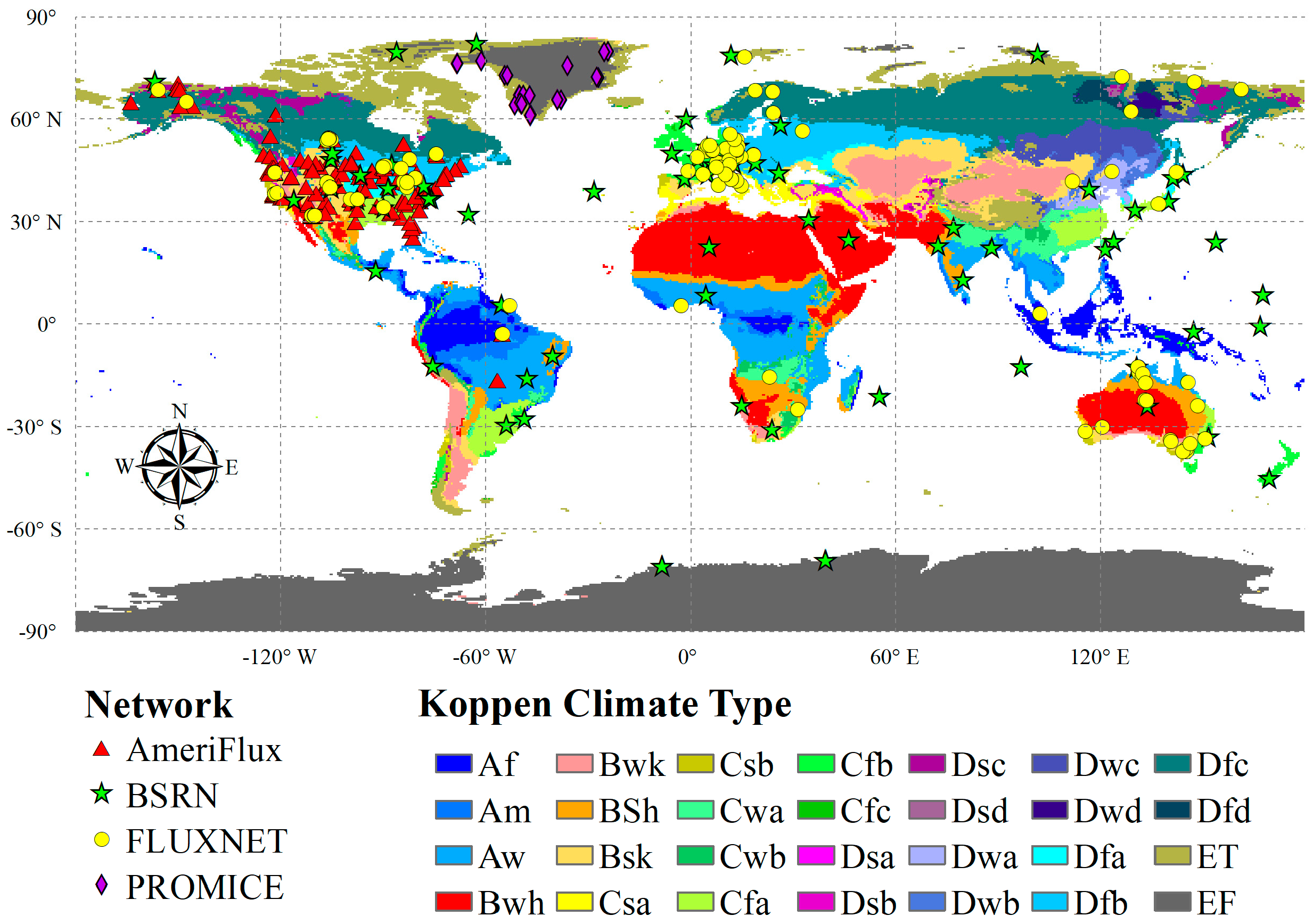
Globally distributed flux networks provide continuous measurements of surface longwave radiation, enabling the validation of a wide range of surface longwave radiation products. In this study, we collected three years of ground measurements from 409 flux stations at four flux networks situated in diverse climatic regions and biomes to verify the accuracy of the CERES-SSF clear-sky SLDR under ATI conditions. They range in altitude from −5 to 3513 m and in latitude from 70.65°S to 82.49°N. These stations include 186 stations from AmeriFlux [21], 126 stations from FLUXNET [22], 27 stations from Programme for Monitoring of the Greenland Ice Sheet (PROMICE) [23], and 70 stations from the Baseline Surface Radiation Network (BSRN) [24]. Longwave radiation at these stations was measured by the Kipp & Zonen net radiometers (CNR1, CNR4, and CNR1-lite), for which the manufacturer reports a sensor uncertainty of $~\pm$10% [23,25]. The global distribution of these stations is shown in Figure 1, and Table A1 provides detailed information on site short names, latitude, longitude, and the time periods used.

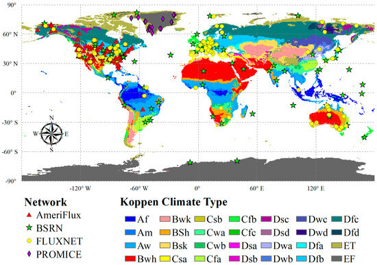
Figure 1. The geographical distribution of the flux stations selected from four flux networks and various climatic types. Symbols represent the different observation networks. The background map shows the Koppen-Geiger climate classification [26].

2.3. MODIS Atmospheric Profile Product

The Moderate Resolution Imaging Spectroradiometer (MODIS) Level-2 Atmospheric Profile product (MxD07_L2) [27] is produced by the MODIS Atmosphere Science Team. The MxD07 utilizes 15 infrared channels to precisely retrieve high spatial resolution atmospheric temperature and moisture profiles, supporting detailed atmospheric analysis [27,28]. The dataset includes land surface temperature, pressure, elevation, cloud mask, and several other parameters such as dew point temperature, atmospheric temperature, and geopotential height for 20 fixed pressure levels: 1000, 950, 920, 850, 780, 700, 620, 500, 400, 300, 250, 200, 150, 100, 70, 50, 30, 20, 10, and 5 hPa. These parameters are generated continuously, day and night, at a 5 × 5 grid of 1 km pixels, provided that at least nine fields of view are cloud-free. This study uses the MODIS atmospheric temperature profile to identify ATI.

Since the MxD07 profiles are provided at 20 standard pressure levels, we implemented a truncation method to ensure physical consistency with the actual topography. For each profile, we utilized the surface pressure provided by MxD07 to truncate the profile. Any standard pressure levels where the pressure exceeded the surface pressure were removed. This is critical for ensuring that only valid atmospheric levels above the ground are used. When the surface pressure exceeded 1000 hPa, we extrapolated the profiles to the surface pressure level using the data from the two lowest available levels [17].

2.4. Methods

2.4.1. ATI Profile Identification

ATI occurs when atmospheric temperature increases with altitude from the surface, and there are several methods to identify it [29]. Kahl [30] and Serreze et al. [31] used the first-order temperature derivatives of sounding data to detect low-level inversions. Starting at the surface, for any two contiguous measurement levels, ${\mathrm{z}}_2$ (unit: m) and ${\mathrm{z}}_1$ (where ${\mathrm{z}}_2>{\mathrm{z}}_1$), with corresponding temperatures ${\mathrm{T}}_2$ and ${\mathrm{T}}_1$, the first-order temperature derivative is defined as follows:

$$\mathrm{\theta }(\mathrm{z})={\displaystyle \frac{\mathrm{d}\mathrm{T}}{\mathrm{d}\mathrm{z}}}={\displaystyle \frac{{\mathrm{T}}_2-{\mathrm{T}}_1}{{\mathrm{z}}_2-{\mathrm{z}}_1}}$$

(9)

The profile is designated as an ATI profile when any derivative is positive. The intensity of the ATI profile (K/100 m) is characterized as

$$\mathrm{A}\mathrm{T}\mathrm{I}={\displaystyle \frac{\mathrm{\Delta }\mathrm{T}}{\mathrm{\Delta }\mathrm{H}}}={\displaystyle \frac{{\mathrm{T}}_2-{\mathrm{T}}_1}{{\mathrm{H}}_2-{\mathrm{H}}_1}}\times 100$$

(10)

where ${\mathrm{T}}_2$ and ${\mathrm{T}}_1$ are the air temperature (K) at the bottom and the top of the inversion layer, and the height (m) at the corresponding levels are ${\mathrm{H}}_2$ and ${\mathrm{H}}_1$, respectively. Fochesatto [32] advanced this work by developing a numerical method for determining multi-layered temperature inversions that could deduce neutral thermal states, isothermal conditions, and surface-based inversions in a temperature profile. Combining the methodology proposed by Kahl [30] and Fochesatto [32], Zhang et al. [33] introduced a more comprehensive detection framework for ATIs from the surface up to 3 km. Their methodology embedded non-inversion layers less than 100 m in thickness within the overall inversion structure, while requiring the inversion depth to exceed 20 m and strength stronger than 0.5 K. The high-resolution vertical temperature profiles from radiosondes were widely employed to detect inversions. Despite the merit of sounding data in capturing atmospheric vertical structure, the radiosonde is sparse and unevenly distributed. In addition, this approach is labor-intensive, costly, and insufficient for monitoring large areas of the atmosphere. The advent of remote sensing technology has revolutionized the identification of ATIs on regional and global scales. Satellite-based methods now offer a highly effective method to obtain continuous atmospheric profiles with superior spatiotemporal resolution.

In this study, a method was developed to detect ATIs from the MODIS atmospheric profile product. The temperature lapse rate between the three lowest effective atmospheric temperature levels from the surface is first calculated. The lapse rates between the first three levels are given by

$${\mathrm{\gamma }}_1={\displaystyle \frac{{\mathrm{T}}_2-{\mathrm{T}}_1}{{\mathrm{z}}_2-{\mathrm{z}}_1}} \mathrm{a}\mathrm{n}\mathrm{d} {\mathrm{\gamma }}_2={\displaystyle \frac{{\mathrm{T}}_3-{\mathrm{T}}_2}{{\mathrm{z}}_3-{\mathrm{z}}_2}}$$

(11)

where ${\mathrm{T}}_{\mathrm{i}}$ and ${\mathrm{z}}_{\mathrm{i}}$ denote the temperature and altitude of the $\mathrm{i}-\mathrm{t}\mathrm{h}$ level, respectively. If the two continuous lapse rates are greater than or equal to zero $({\mathrm{\gamma }}_1\ge 0 \mathrm{a}\mathrm{n}\mathrm{d} {\mathrm{\gamma }}_2\ge 0)$, an ATI profile is identified.

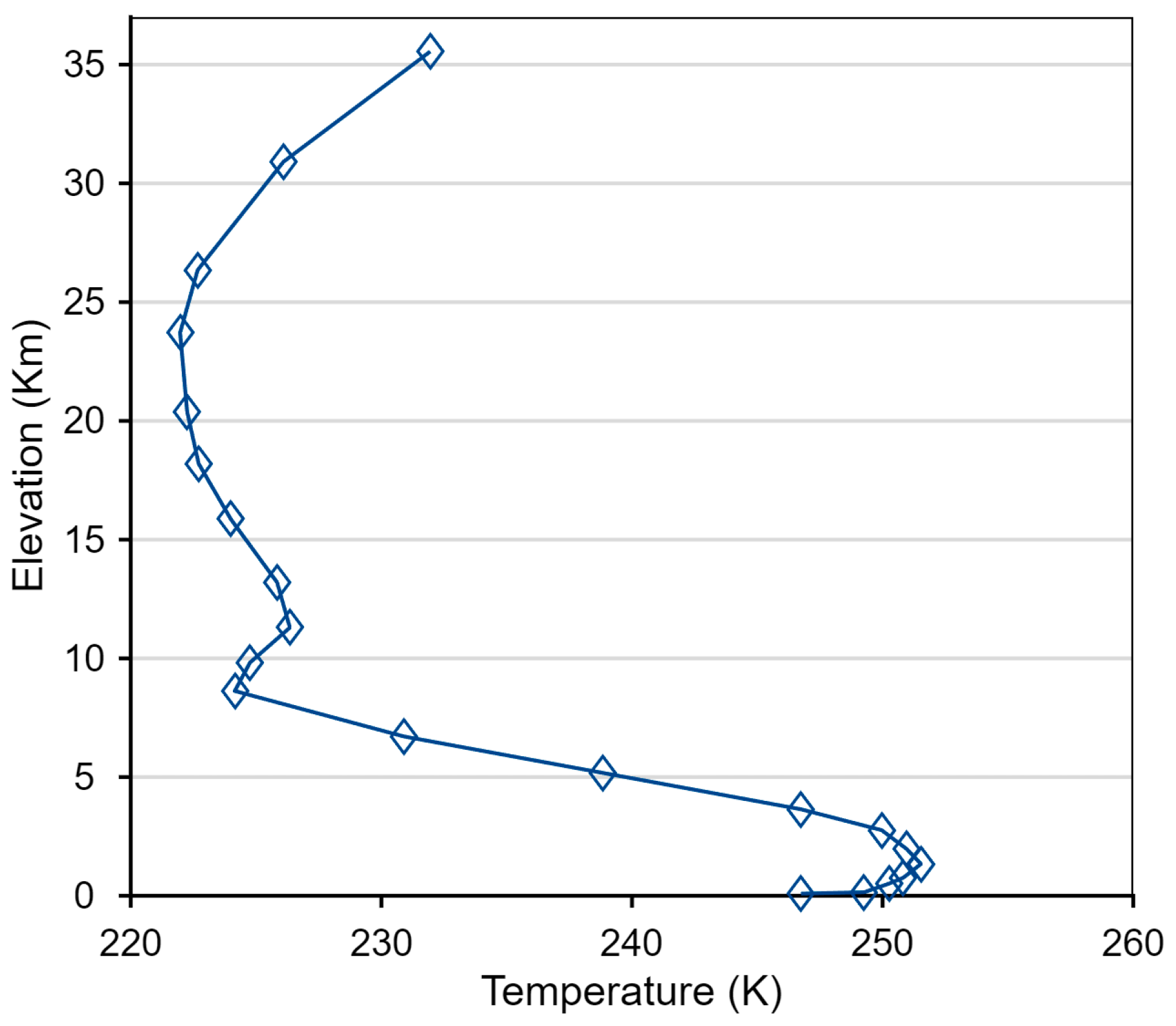
The inversion top is defined as the level showing a lapse rate less than zero. We obtained 363,396 normal temperature profiles and 90,914 ATI profiles collocated with the geographical locations of the 409 flux stations. Figure 2 shows an example of an ATI profile. The air temperature increases with altitude near the surface boundary.

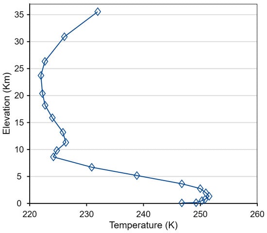
Figure 2. An example of the identified MODIS ATI profile.

2.4.2. Data Processing

Only the pixels labeled as “confident clear” in the MxD07 cloud mask were retained to identify the clear-sky near-surface ATI. The ground-measured SLDR was compared to the collocated CERES SLDR without taking any temporal and spatial averaging.

Several steps are required to spatiotemporally match the ground measurements with CERES-SSF SLDR data. For temporal matching, the time difference between the station observations and the overpass time of satellite data should not exceed 15 min. Initially, we downloaded the MxD07 data according to the location of flux stations. Secondly, using the timestamps from the MODIS–ground temporal matching as the benchmark, we selected the clear-sky CERES SSF SLDR according to the MxD07 clear-sky pixels. The MODIS atmospheric profile, the SSF clear-sky SLDR, and the ground-measured SLDR at the same time are obtained. Spatial matching was performed by calculating the great-circle distance between the station geolocation and the satellite pixel. For the SSF product, which consists of multiple footprints, we selected all footprints with centers located within a 20 km radius of a ground station, whereas for the MxD07, which is stored in a latitude and longitude grid, each station is exclusively matched up with MODIS pixels within 5 km of the spherical distance.

$$\mathrm{d}=2\mathrm{R}·\arcsin \left[\sqrt{{\sin }^2({\displaystyle \frac{{\mathrm{\varphi }}_2-{\mathrm{\varphi }}_1}{2}})+\cos {\mathrm{\varphi }}_1\cos {\mathrm{\varphi }}_2{\sin }^2({\displaystyle \frac{{\mathrm{\phi }}_2-{\mathrm{\phi }}_1}{2}})}\right]$$

(12)

where $\mathrm{d}$ is the great circle distance between two points, $\mathrm{R}$ is the Earth’s radius (approximately 6378.14 km), and ${\mathrm{\varphi }}_{\mathrm{i}}$ and ${\mathrm{\phi }}_{\mathrm{i}}$ are the longitude and latitude of the point (in radians).

To minimize the effects of cloud contamination and ground measurement uncertainties [4,34], and to obtain robust statistics for SLDR validation, we removed outliers from the SLDR matched values using the “3σ Hampel identifier” method [35]. Specifically, we calculated the difference between the clear-sky SSF SLDR and the ground-measured SLDR. If the sample deviates more than three standard deviations from the median, it is considered an outlier and removed from the dataset. The standard deviation is calculated as follows:

$$\mathrm{S}=1.4826\times \mathrm{m}\mathrm{e}\mathrm{d}\mathrm{i}\mathrm{a}\mathrm{n}\left\{\left|{\mathrm{x}}_{\mathrm{i}}-{\mathrm{x}}_{\mathrm{m}}\right|\right\}$$

(13)

where ${\mathrm{x}}_{\mathrm{i}}$ represents the difference between the paired clear-sky CERES-SSF SLDR value and the ground-measured value, and ${\mathrm{x}}_{\mathrm{m}}$ signifies the median of $\left\{{\mathrm{x}}_{\mathrm{i}}\right\}$. The coefficient 1.4826 converts the median absolute deviation into an unbiased standard deviation estimate for normally distributed data. The term $\mathrm{S}$ refers to the standard deviation. Additionally, SLDR samples with ${\mathrm{x}}_{\mathrm{i}}$ less than ${\mathrm{x}}_{\mathrm{m}}-3\mathrm{S}$ or greater than ${\mathrm{x}}_{\mathrm{m}}+3\mathrm{S}$ are considered outliers and excluded. Note that the quality control and outlier removal process was performed independently for each CERES model (A, B, and C) on a site-by-site basis, resulting in varying final sample sizes. Consequently, we obtained 4264, 34,771, and 35,003 matchups for Models A, B, and C under ATI conditions.

2.4.3. Evaluation Metrics

In this paper, the mean difference between the predicted and observed SLDRs (Bias), the Root Mean Square Error (RMSE), and the determination coefficient (R²) were employed as evaluation metrics for assessing the performance of SLDR estimates. The formulas are as follows:

$$\mathrm{B}\mathrm{i}\mathrm{a}\mathrm{s}={\displaystyle \frac{1}{\mathrm{N}}}{\displaystyle \sum _{\mathrm{i}=1}^{\mathrm{N}}({\mathrm{y}}_{\mathrm{s}}-{\mathrm{y}}_{\mathrm{o}})}$$

(14)

$$\mathrm{R}\mathrm{M}\mathrm{S}\mathrm{E}={\left({\displaystyle \frac{1}{\mathrm{N}}}{{\displaystyle \sum _{\mathrm{i}=1}^{\mathrm{N}}({\mathrm{y}}_{\mathrm{s}}-{\mathrm{y}}_{\mathrm{o}})}}^2\right)}^{1/2}$$

(15)

$${\mathrm{R}}^2=1-{{\displaystyle \sum _{\mathrm{i}=1}^{\mathrm{N}}({\mathrm{y}}_{\mathrm{s}}-{\mathrm{y}}_{\mathrm{o}})}}^2/{\displaystyle \sum _{\mathrm{i}=1}^{\mathrm{N}}{({\mathrm{y}}_{\mathrm{o}}-\overline{{\mathrm{y}}_{\mathrm{o}}})}^2}$$

(16)

where $\mathrm{N}$ is the number of observations, ${\mathrm{y}}_{\mathrm{s}}$ represents the CERES-SSF clear-sky SLDR values, and ${\mathrm{y}}_0$ is the ground-measured SLDR values.

3. Results

3.1. Overall Performance

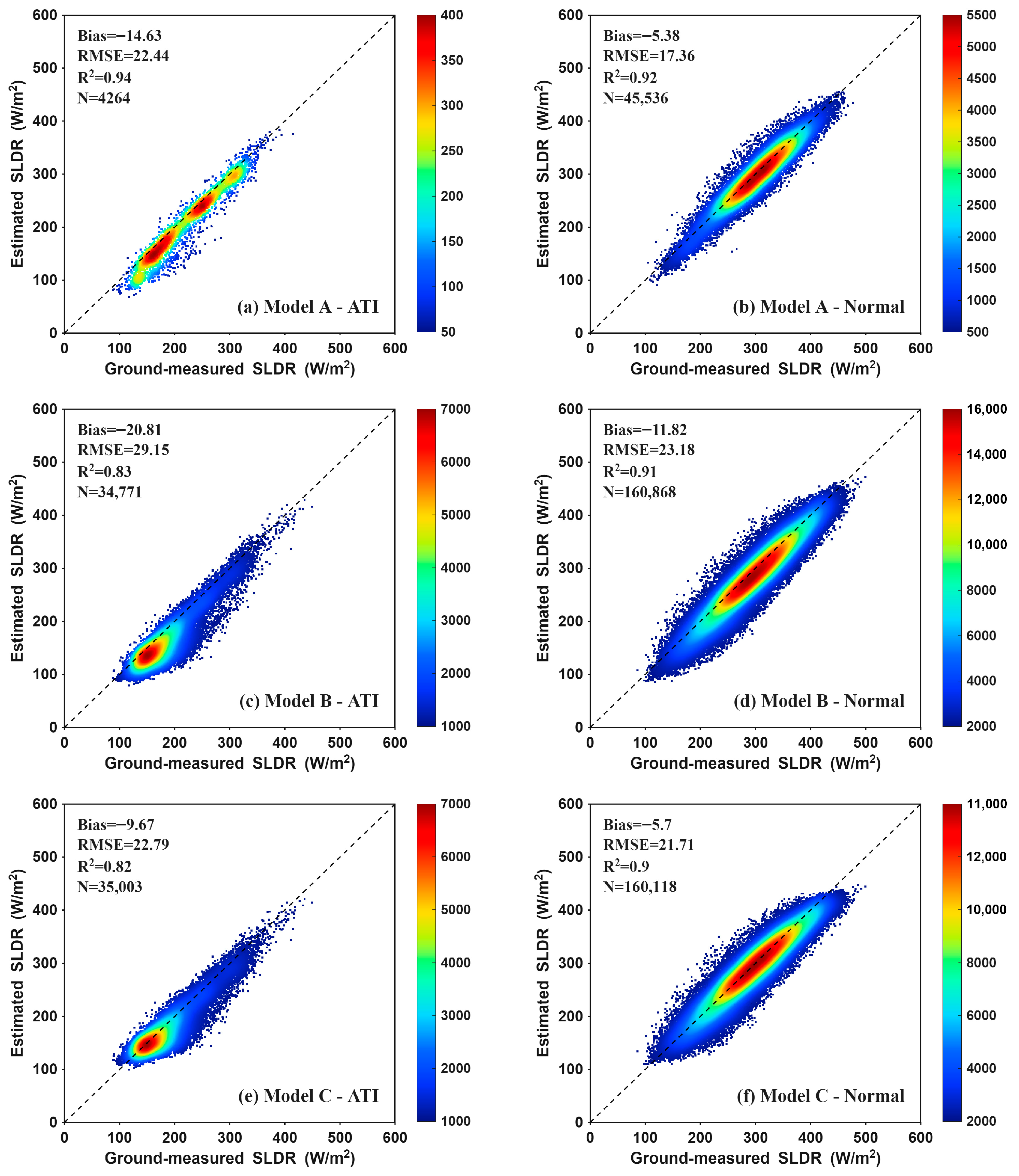
Figure 3 shows the overall performance of the three models. Under ATI conditions, the SLDR distribution range is relatively narrow, clustering primarily between 100 and 250 W/m². This prevalence of lower values is expected, as ATI events occur predominantly in polar regions and during the nighttime. The CERES clear-sky SLDR products are significantly underestimated, resulting in larger negative Biases of −14.63 W/m², −20.81 W/m², and −9.67 W/m² for Models A, B, and C, respectively; the corresponding RMSE values are 22.44 W/m², 29.15 W/m², and 22.79 W/m². On the contrary, the SLDR samples under normal atmospheric temperature conditions span a broader range (100–450 W/m²) and are symmetrically distributed around the 1:1 line, with Biases of −5.38 W/m², −11.82 W/m², and −5.7 W/m², and RMSE values of 17.36 W/m², 23.18 W/m², and 21.71 W/m², respectively. The validation results under normal conditions are consistent with those reported in Kratz et al. [9].

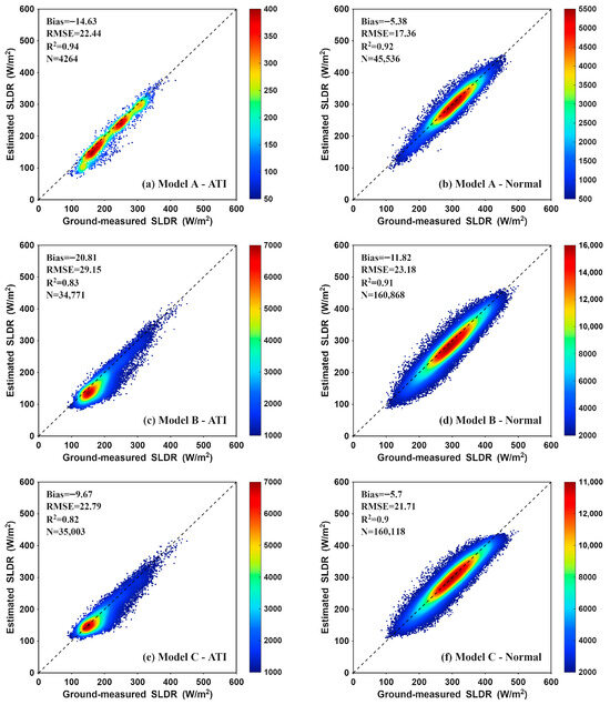
Figure 3. Accuracy of the clear-sky CERES SLDR products under ATI and normal conditions.

In summary, ATI degrades the clear-sky SLDR estimate accuracy. The degradation in Bias/RMSE is approximately 10.0/5.0 W/m² for Models A and B, whereas the values for Model C are approximately 5.0/1.0 W/m². In contrast to Models A and B, the impact of ATI on Model C is less pronounced, as it possesses a certain resistance to ATI.

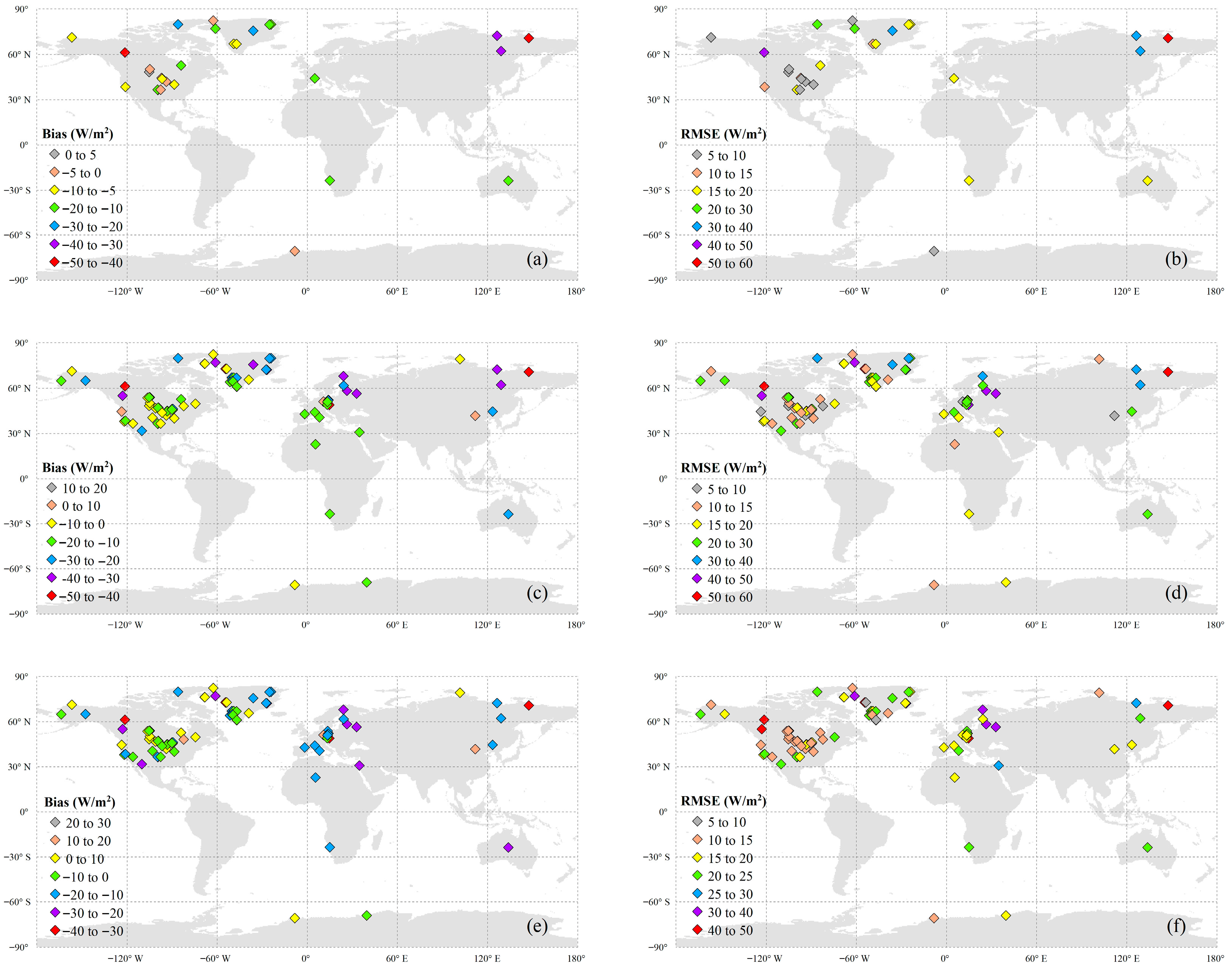
Figure 4 shows the spatial distribution of the validation results at each flux station under ATI conditions except for those with too few samples (the number of samples is less than 30). In North America, the Biases of Model A and Model B are mainly within the range of 0 to –20 W/m², and that of Model C predominantly falls within ±10 W/m². Accordingly, the RMSE values of Models A and C are mostly distributed between 5 and 20 W/m² and 10 and 25 W/m², respectively, while the RMSE value of Model B is primarily concentrated in 5–30 W/m². In Europe, the Biases of Models A are primarily between –20 and −10 W/m², with many of Model B’s Biases clustered below –30 W/m². In contrast, Model C’s Bias ranges from –30 to –10 W/m². The corresponding RMSE values are generally 15–20 W/m² for Model A; 15–40 W/m² for Models B and C, with values above 30 W/m² at most stations. Despite the limitation of a single flux site in Australia, all Models exhibit a pronounced negative Bias (exceeding –10 W/m²) in SLDR, accompanied by RMSEs of 15–30 W/m². For the African sites, Model biases are predominantly in the –20 to –10 W/m² range, with respective RMSE values of 15–20, 10–20, and 15–25 W/m². In northeastern Asia (120°–180°E), a similar pattern shows Biases exceeding –20 W/m². While the RMSE of Models A and B exceeds 30 W/m², that of Model C falls between 15 and 30 W/m². In Antarctica, Models A, B, and C exhibit Biases of −5 to 0, 0 to −20, and −10 to 10 W/m², respectively. The corresponding RMSE ranges are 5–10 W/m² for Model A and 10–20 W/m² for both Models B and C. These findings are consistent with the overall accuracies presented in Figure 3a,c,e.

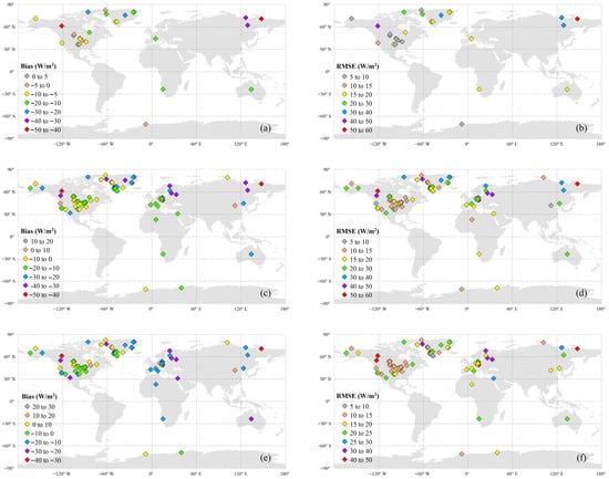
Figure 4. Spatial distribution of the validation results at each station under ATI conditions. (a) Bias and (b) RMSE for Model A, (c) Bias and (d) RMSE for Model B, (e) Bias and (f) RMSE for Model C.

3.2. Results for Polar and Non-Polar Region

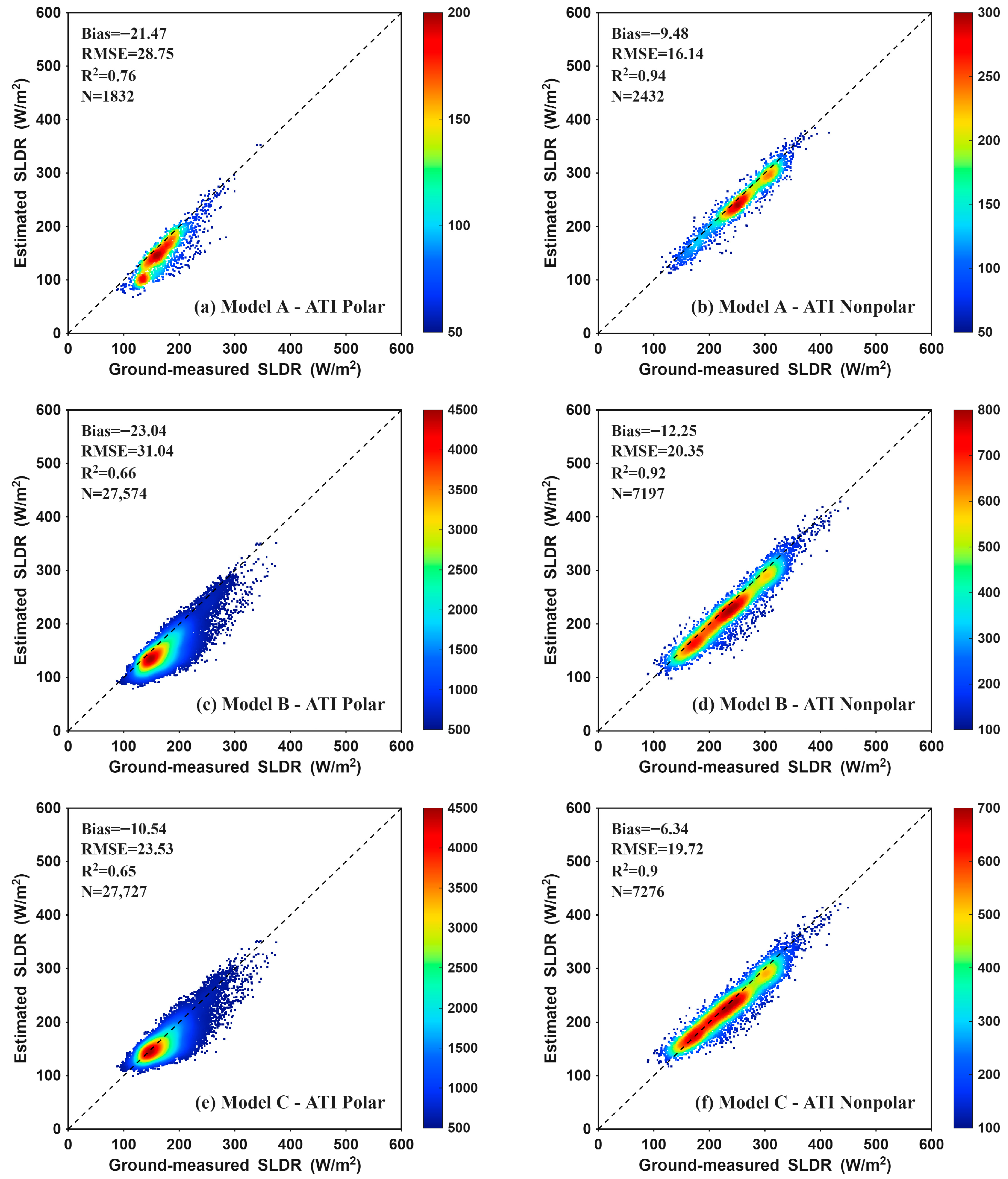
The pronounced vulnerability and intricate environmental dynamics of polar regions (>60° latitude), distinct from mid-latitudes, necessitate a thorough assessment of the effects of ATI on CERES SLDR products. The validation results are provided in Figure 5, which shows the scatter density distribution of the validation results for polar and non-polar regions under ATI conditions. For Model A, a distinct characteristic is observed during polar ATI events, where SLDR values tend to cluster within a relatively narrow and lower range (approximately 100–250 W/m²). This feature is less pronounced in Models B and C. This prevalence of low SLDR values stems from the intense surface LW radiative cooling, which is compounded by the inherently low ambient atmospheric temperatures and scarce water vapor content characteristic of polar environments.

Figure 5. Validation results of the clear-sky CERES SLDR products for polar and non-polar regions under ATI conditions.

Table 1 shows the performance of CERES clear-sky SLDR products in polar and non-polar regions under ATI and normal conditions, respectively. ATI further degrades product accuracy in both polar and non-polar regions, as evidenced by increased negative Biases and RMSEs.

Table 1. The accuracy of Models A, B, and C for polar and non-polar regions under ATI and normal conditions, respectively.

SLDR	Metric	Polar		Non-Polar
		ATI	Normal	ATI	Normal
Model A	Bias	−21.47	−13.32	−9.48	−4.70
	RMSE	28.75	18.05	16.14	17.30
	R2	0.76	0.95	0.94	0.89
	No.	1832	3573	2432	41,963
Model B	Bias	−23.04	−22.05	−12.25	−9.26
	RMSE	31.04	30.23	20.35	21.06
	R2	0.66	0.85	0.92	0.90
	No.	27,574	32,134	7197	128,734
Model C	Bias	−10.54	−10.93	−6.34	−4.37
	RMSE	23.53	24.92	19.72	20.81
	R2	0.65	0.82	0.90	0.88
	No.	27,727	32,550	7276	127,568

In polar regions, the Bias/RMSE values for Models A, B, and C are −13.32/18.05 W/m², −22.05/30.23 W/m², and −10.93/24.92 W/m² under normal atmospheric temperature conditions. Under ATI conditions, these values change to −21.47/28.75 W/m², −23.04/31.04 W/m², and −10.54/23.53 W/m². A comparison of these conditions reveals distinct model behaviors. Model A exhibits the most significant performance degradation, with its absolute Bias and RMSE increasing by 8.15 W/m² and 10.70 W/m², respectively. Model B shows a minor decline, with increases of 0.99 W/m² in Bias and 0.81 W/m² in RMSE. In contrast, Model C demonstrates exceptional stability and robustness; its absolute Bias remains nearly unchanged, while its RMSE improves by 1.39 W/m² under ATI conditions. These results suggest that Model C is the most robust choice for operational retrieval in polar regions prone to temperature inversions.

In non-polar regions, the impact of ATI is primarily manifested in the intensification of systematic negative biases. Models A, B, and C saw their negative Biases increase by 4.78 W/m², 2.99 W/m², and 1.97 W/m², respectively. Notably, Model A in non-polar regions shows a twofold increase in negative bias when ATI occurs, suggesting that the model’s deficiency is physically linked to the vertical temperature structure.

Moreover, a notable pattern emerges: CERES models substantially underestimate SLDR in polar regions compared to non-polar regions, regardless of ATI presence. This occurs because clear-sky SLDR is influenced by both near-surface air temperature and water vapor content. Due to the extremely low water vapor content in polar regions [36], SLDR tends to be underestimated there, and as shown in Table 1, the presence of ATIs further exacerbates this underestimation [9].

3.3. Results for Daytime and Nighttime

The accurate estimation of SLDR is subject to diurnal variations in atmospheric processes. While daytime conditions are largely governed by solar radiative input, nighttime atmospheric stability often promotes the development of ATIs, which can substantially alter the near-surface radiative environment. Evaluating daytime and nighttime accuracy separately allows for a more nuanced understanding of how ATIs influence the Models.

Detailed validation results for daytime and nighttime are presented in Table 2. In general, the occurrence of ATI leads to a degradation in SLDR estimate accuracy, but the magnitude of this impact varies significantly by Model and time of day. During the daytime, Models A and B exhibit a clear decline in performance under ATI conditions. For instance, the negative Bias for Model A widened from −3.17 to −12.93 W/m², while its RMSE increased from 17.20 W/m² to 21.53 W/m². Similarly, Model B sees its negative Bias exacerbate from −11.29 to −15.82 W/m² with RMSE rising from 23.30 to 26.10 W/m². In contrast, Model C demonstrates remarkable stability during the day, with its Bias remaining virtually unchanged (from −4.68 to −4.44 W/m²) and only a negligible increase in RMSE (from 21.65 to 22.09 W/m²), suggesting it is robust against daytime ATI events.

Table 2. The accuracy of Models A, B, and C for daytime and nighttime under ATI and normal conditions, respectively.

SLDR	Metric	Daytime		Nighttime
		ATI	Normal	ATI	Normal
Model A	Bias	−12.93	−3.17	−15.20	−7.77
	RMSE	21.53	17.20	22.74	17.53
	R2	0.81	0.93	0.95	0.89
	No.	1077	23,686	3187	21,850
Model B	Bias	−15.82	−11.29	−21.98	−12.53
	RMSE	26.10	23.30	29.83	23.02
	R2	0.81	0.92	0.84	0.90
	No.	6614	92,731	28,157	68,137
Model C	Bias	−4.44	−4.68	−10.86	−7.06
	RMSE	22.09	21.65	22.94	21.78
	R2	0.79	0.91	0.83	0.88
	No.	6491	90,961	28,512	69,157

During nighttime, however, the negative impact of ATI becomes more systematic across all models. Model A’s Bias drops further from −7.77 to −15.20 W/m². Model B experiences the most severe degradation, with its Bias plunging from −12.53 to −21.98 W/m² and RMSE increasing significantly from 23.02 to 29.83 W/m². Even Model C, which was stable during the day, shows a noticeable decline at night, with Bias shifting from −7.06 to −10.86 W/m², although its RMSE increase remains moderate (1.16 W/m²).

Furthermore, ATI events are found to occur at significantly higher frequency during the nighttime compared to the daytime. This may be attributed to the imbalance among SLUR, shortwave downward radiance (SWDR) and SLDR [37]. In the absence of SWDR input at night, the surface typically experiences a net loss of energy due to continuous SLUR exceeding the SLDR, leading to surface cooling rapidly, fostering the development of a stable ATI where the surface is colder than the air directly above it.

4. Discussion

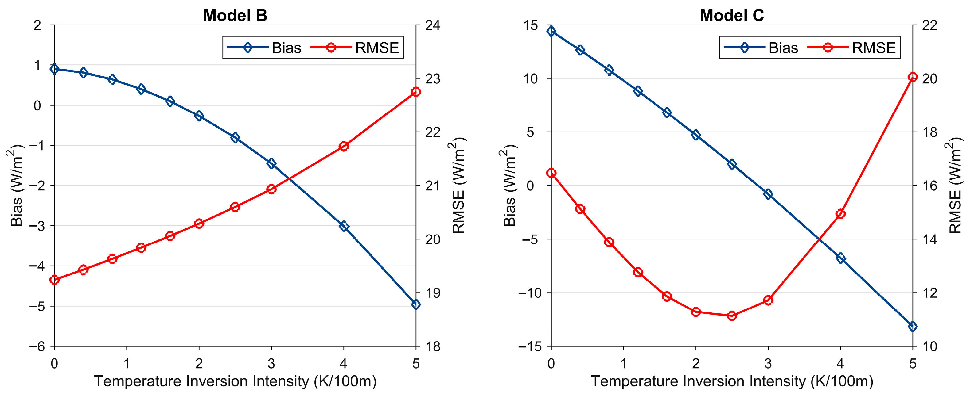
SLDR is dominated by near-surface air temperature and water vapor content under clear-sky conditions [5]. This is the physical basis for LW models. However, nighttime radiative cooling and extremely dry conditions in polar and high-altitude regions can cause the surface to cool faster than the air above, forming strong temperature inversions, particularly in polar and high-altitude regions. The surface skin temperature can be up to 20–30 K lower than that of the lowest atmospheric layers, as the extremely dry air allows the surface to radiate almost directly to space, resulting in a substantial underestimation of SLDR [9]. Generally, the CERES Models implicitly assume a typical lapse-rate structure, and the ATI condition was not incorporated into the developed LW Models. Hence, they systematically underestimate SLDR in regions where strong, persistent ATIs are common. To assess the influence of ATI on the SLDR estimate, we performed a sensitivity analysis utilizing version 2.4 of the Santa Barbara DISORT Atmospheric Radiative Transfer (SBDART) model [38]. The atmospheric profile inputs for these simulations are selected from the latest Thermodynamic Initial Guess Retrieval (TIGR2000) [39] database, which encompasses a wide range of global atmospheric conditions, featuring water vapor content from 0.1 to 8 g/cm² and surface temperature from 231 to 315 K. The profiles with relative humidity greater than 90% at any single level or greater than 85% at two consecutive levels were removed from the TIGR database [17]. The remaining clear-sky profiles were subsequently categorized as either normal or ATI according to the near-surface air temperature gradient, in accordance with the algorithm outlined in Section 2.4. Ultimately, we obtained 349 ATI profiles and 1032 normal profiles under the clear-sky conditions, respectively. Due to the limited variation in ATIIs in the TIGR atmospheric profiles, which is inadequate for an extensive sensitivity analysis, we did not use the selected ATI profiles but manually altered the normal atmospheric temperature profile to an anomalous one. For each normal profile, the initial bottom-level air temperature was preserved. Then, the temperatures at the first and second atmospheric levels immediately above the surface were calculated based on the air temperature inversion intensity (ATII) and replaced the original values. Subsequently, we retrieved the SLDR with both the normal and modified ATI atmospheric profiles, adopting the coefficients from the CERES LW Models as detailed in Section 2.1. The SDLR simulated by SBDART was treated as the true value and used to evaluate the SDLR calculated by the CERES LW algorithms.

Figure 6 displays the resultant Biases and RMSEs of SLDR retrieval for different ATIIs. The Bias of models shows a distinct sensitivity to the ATII. Model B exhibits a gradual reduction in Bias from 0.79 W/m² under normal conditions to −4.96 W/m² at the ATII of 5 K/100 m. A more apparent tendency is evident for Model C, of which Bias transits from a considerable positive value of 15.94 W/m² to a notable negative value of −13.17 W/m². The continual drop in Bias, resulting in negative Biases at high ATI strengths, suggests that both models tend to underestimate SLDR under robust inversion conditions.

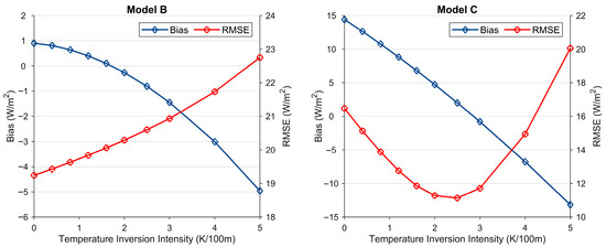
Figure 6. The Bias and RMSE of the retrieved SLDR under various ATI intensities.

Concerning the RMSE, Model B displays a consistent increase with ascending ATII, rising from 18.65 W/m² to 22.75 W/m². For Model C, the SLDR estimate remains nearly unchanged since the input variables (surface temperature and column precipitable water vapor) are consistent throughout. As the ATII escalates, the simulated “true” SLDR value rises, contributing to a reduction in the model’s initial overestimation, which ultimately shifts to a significant underestimation. Consequently, the Bias transitions from positive to negative. This tendency is explicitly reflected in the RMSE, which first diminishes from 17.56 W/m² to a minimum of 11.13 W/m² at the ATII of 2.5 K/100 m. Afterward, as ATII further advances, the RMSEs sharply rise to around 20 W/m².

The rise in air temperature causes increased emissions from the atmosphere, the effective atmospheric temperature derived from constant weighted air temperature in Model B fails to capture these changes, making it underestimate the SLDR. Meanwhile, Model C omits the thermal radiation emitted by the atmosphere, resulting in a systematic negative bias.

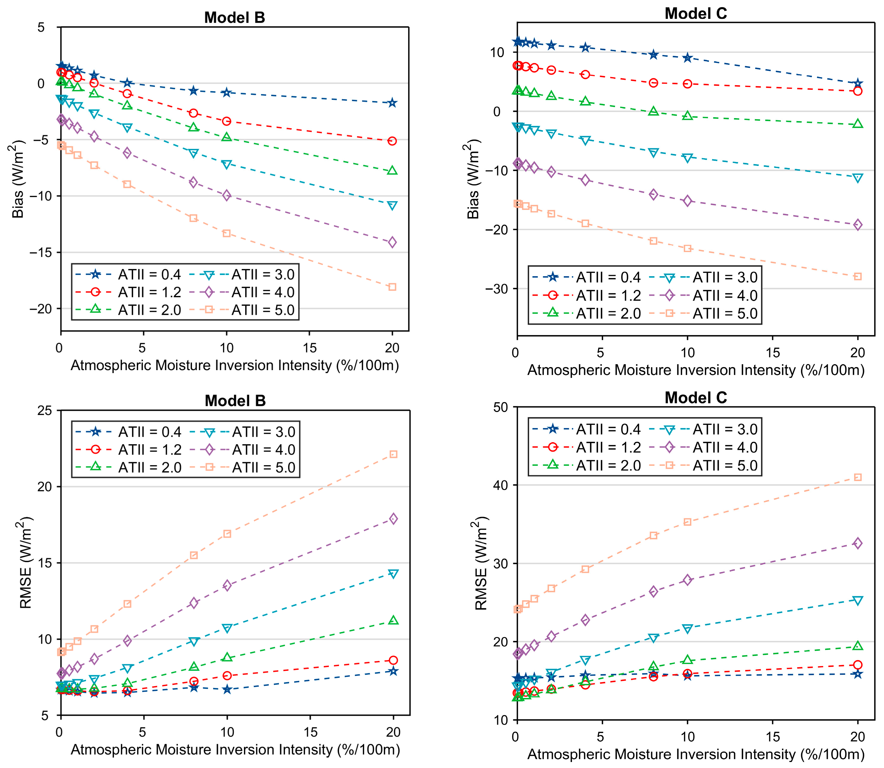
The moisture inversion frequently coincides with atmospheric temperature inversion. We investigated the resulting changes in SLDR during the simultaneous occurrence of both inversion types. The atmospheric moisture inversion intensity (AMII, %/100 m) is defined as:

$$\mathrm{A}\mathrm{M}\mathrm{I}\mathrm{I}={\displaystyle \frac{{\mathrm{W}}_2-{\mathrm{W}}_1}{{\mathrm{W}}_1}}{\displaystyle \frac{1}{({\mathrm{H}}_2-{\mathrm{H}}_1)}}\times 100$$

(17)

where ${\mathrm{W}}_1$ and ${\mathrm{W}}_2$ is the water vapor content (g/m³) at the bottom and the top of the inversion layer, the height (m) at the corresponding level is ${\mathrm{H}}_2$ and ${\mathrm{H}}_1$, respectively.

Figure 7 shows the resulting Biases and RMSEs of the retrieved SLDR for various AMIIs. It demonstrates that the RMSEs of both Models grow when the AMI intensifies, and this upward trend is more evident at higher ATI intensities. Both models’ Biases follow a trend of increasing negatively with the strength of the inversion. These results emphasize the complexities of obtaining SLDR in atmospheres with anomalous temperature and moisture profiles. The contemporaneous existence of these inversions significantly reduces the accuracy of SLDR estimates, underlining the necessity for retrieval methods that can properly account for such anomalous atmospheric circumstances.

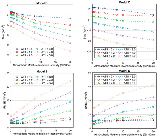
Figure 7. Bias and RMSE of retrieved SLDR for different intensities of atmospheric moisture inversion.

5. Conclusions

This paper comprehensively investigated the accuracy of the clear-sky CERES SLDR products under ATI conditions, utilizing ground-measured SLDR collected from 409 flux stations across four radiation flux networks. Under ATI conditions, the accuracy of all three Models degraded in the polar and non-polar regions, as well as during the daytime and nighttime.

Under ATI conditions, the Bias/RMSE increases by approximately 10.0/5.0 W/m² for Models A and B, 5.0/1.0 W/m² for Model C, compared to those obtained under normal conditions. Both the Bias and RMSE of Models B and C are sensitive to the ATI intensity. The Bias decreases with the increase in ATI intensity, but RMSE behaves differently with the increase in ATI intensity. Both the Bias and RMSE deteriorate with the increase in the concurrent AMII.

This efforts in this study, combined with existing CERES SLDR product validation, provides a thorough evaluation of the CERES SLDR product, offering strong guidance for its users. Furthermore, these findings mark a crucial step toward refining our understanding of ATI’s impact on clear-sky SLDR estimates. We must make efforts to advance the current algorithm, most critically, by systematically integrating additional, well-quantified influencing factors.

References

- Liang, S.; Cheng, J.; Jia, K.; Jiang, B.; Liu, Q.; Xiao, Z.; Yao, Y.; Yuan, W.; Zhang, X.; Zhao, X. The Global Land Surface Satellite (GLASS) Product Suite. Bull. Am. Meteorol. Soc. 2021, 102, E323–E337. [Google Scholar] [CrossRef]
- Stephens, G.L.; Wild, M.; Stackhouse, P.W.; L’Ecuyer, T.; Kato, S.; Henderson, D.S. The Global Character of the Flux of Downward Longwave Radiation. J. Clim. 2012, 25, 2329–2340. [Google Scholar] [CrossRef]
- Zeng, Q.; Cheng, J.; Sun, H.; Dong, S. An Integrated Framework for Estimating the Hourly All-Time Cloudy-Sky Surface Long-Wave Downward Radiation for Fengyun-4A/AGRI. Remote Sens. Environ. 2024, 312, 114319. [Google Scholar] [CrossRef]
- Cheng, J.; Liang, S.; Wang, W.; Guo, Y. An Efficient Hybrid Method for Estimating Clear-Sky Surface Downward Longwave Radiation from MODIS Data: A Hybrid Method for Estimating LWDN. J. Geophys. Res. Atmos. 2017, 122, 2616–2630. [Google Scholar] [CrossRef]
- Gupta, S.K. A Parameterization for Longwave Surface Radiation from Sun-Synchronous Satellite Data. J. Clim. 1989, 2, 305–320. [Google Scholar] [CrossRef]
- Pinker, R.T.; Tarpley, J.D.; Laszlo, I.; Mitchell, K.E.; Houser, P.R.; Wood, E.F.; Schaake, J.C.; Robock, A.; Lohmann, D.; Cosgrove, B.A.; et al. Surface Radiation Budgets in Support of the GEWEX Continental-scale International Project (GCIP) and the GEWEX Americas Prediction Project (GAPP), Including the North American Land Data Assimilation System (NLDAS) Project. J. Geophys. Res. 2003, 108, 2002JD003301. [Google Scholar] [CrossRef]
- Zhang, Y.; Rossow, W.B.; Lacis, A.A. Calculation of Surface and Top of Atmosphere Radiative Fluxes from Physical Quantities Based on ISCCP Data Sets: 1. Method and Sensitivity to Input Data Uncertainties. J. Geophys. Res. 1995, 100, 1149–1165. [Google Scholar] [CrossRef]
- Kratz, D.P.; Gupta, S.K.; Wilber, A.C.; Sothcott, V.E. Validation of the CERES Edition 2B Surface-Only Flux Algorithms. J. Appl. Meteorol. Climatol. 2010, 49, 164–180. [Google Scholar] [CrossRef]
- Kratz, D.P.; Gupta, S.K.; Wilber, A.C.; Sothcott, V.E. Validation of the CERES Edition-4A Surface-Only Flux Algorithms. J. Appl. Meteorol. Climatol. 2020, 59, 281–295. [Google Scholar] [CrossRef]
- Wielicki, B.A.; Barkstrom, B.R.; Baum, B.A.; Charlock, T.P.; Green, R.N.; Kratz, D.P.; Lee, R.B.; Minnis, P.; Smith, G.L.; Wong, T.; et al. Clouds and the Earth’s Radiant Energy System (CERES): Algorithm Overview. IEEE Trans. Geosci. Remote Sens. 1998, 36, 1127–1141. [Google Scholar] [CrossRef]
- Cheng, J.; Zeng, Q.; Sun, H.; Yamin, G.; Yang, F.; Guo, M.; Wu, C. A Global 1 Km Resolution Daily Surface Longwave Radiation Product from MODIS Satellite Data from 2000–2023. Sci. Data 2025, 12, 736. [Google Scholar] [CrossRef]
- Busetto, M.; Lanconelli, C.; Mazzola, M.; Lupi, A.; Petkov, B.; Vitale, V.; Tomasi, C.; Grigioni, P.; Pellegrini, A. Parameterization of Clear Sky Effective Emissivity under Surface-Based Temperature Inversion at Dome C and South Pole, Antarctica. Antarct. Sci. 2013, 25, 697–710. [Google Scholar] [CrossRef]
- Dupont, J.; Haeffelin, M.; Drobinski, P.; Besnard, T. Parametric Model to Estimate Clear-sky Longwave Irradiance at the Surface on the Basis of Vertical Distribution of Humidity and Temperature. J. Geophys. Res. 2008, 113, 2007JD009046. [Google Scholar] [CrossRef]
- Brutsaert, W. On a Derivable Formula for Long-Wave Radiation from Clear Skies. Water Resour. Res. 1975, 11, 742–744. [Google Scholar] [CrossRef]
- Prata, A.J. A New Long-Wave Formula for Estimating Downward Clear-Sky Radiation at the Surface. Q. J. R. Met Soc. 1996, 122, 1127–1151. [Google Scholar]
- Yu, S.; Xin, X.; Liu, Q.; Zhang, H.; Li, L. An Improved Parameterization for Retrieving Clear-Sky Downward Longwave Radiation from Satellite Thermal Infrared Data. Remote Sens. 2019, 11, 425. [Google Scholar] [CrossRef]
- Cheng, J.; Liang, S.; Shi, J. Impact of Air Temperature Inversion on the Clear-Sky Surface Downward Longwave Radiation Estimation. IEEE Trans. Geosci. Remote Sens. 2020, 58, 4796–4802. [Google Scholar] [CrossRef]
- Inamdar, A.K.; Ramanathan, V. On Monitoring the Atmospheric Greenhouse Effect from Space. Tellus B Chem. Phys. Meteorol. 1997, 49, 216. [Google Scholar] [CrossRef]
- Inamdar, A.K.; Ramanathan, V. Physics of Greenhouse Effect and Convection in Warm Oceans. J. Clim. 1994, 7, 715–731. [Google Scholar] [CrossRef][Green Version]
- Zhou, Y.; Kratz, D.P.; Wilber, A.C.; Gupta, S.K.; Cess, R.D. An Improved Algorithm for Retrieving Surface Downwelling Longwave Radiation from Satellite Measurements. J. Geophys. Res. 2007, 112, D15102. [Google Scholar] [CrossRef]
- Novick, K.A.; Biederman, J.A.; Desai, A.R.; Litvak, M.E.; Moore, D.J.P.; Scott, R.L.; Torn, M.S. The AmeriFlux Network: A Coalition of the Willing. Agric. For. Meteorol. 2018, 249, 444–456. [Google Scholar] [CrossRef]
- Baldocchi, D.; Falge, E.; Gu, L.; Olson, R.; Hollinger, D.; Running, S.; Anthoni, P.; Bernhofer, C.; Davis, K.; Evans, R.; et al. FLUXNET: A New Tool to Study the Temporal and Spatial Variability of Ecosystem–Scale Carbon Dioxide, Water Vapor, and Energy Flux Densities. Bull. Amer. Meteor. Soc. 2001, 82, 2415–2434. [Google Scholar] [CrossRef]
- Fausto, R.S.; van As, D.; Mankoff, K.D.; Vandecrux, B.; Citterio, M.; Ahlstrøm, A.P.; Andersen, S.B.; Colgan, W.; Karlsson, N.B.; Kjeldsen, K.K.; et al. Programme for Monitoring of the Greenland Ice Sheet (PROMICE) Automatic Weather Station Data. Earth Syst. Sci. Data 2021, 13, 3819–3845. [Google Scholar] [CrossRef]
- Driemel, A.; Augustine, J.; Behrens, K.; Colle, S.; Cox, C.; Cuevas-Agulló, E.; Denn, F.M.; Duprat, T.; Fukuda, M.; Grobe, H.; et al. Baseline Surface Radiation Network (BSRN): Structure and Data Description (1992–2017). Earth Syst. Sci. Data 2018, 10, 1491–1501. [Google Scholar] [CrossRef]
- Wang, K.; Dickinson, R.E. Global Atmospheric Downward Longwave Radiation at the Surface from Ground-based Observations, Satellite Retrievals, and Reanalyses. Rev. Geophys. 2013, 51, 150–185. [Google Scholar] [CrossRef]
- Gebirge, V. Handbuch Der Klimatologie. Nature 1932, 130, 43. [Google Scholar] [CrossRef]
- Seemann, S.W.; Li, J.; Menzel, W.P.; Gumley, L.E. Operational Retrieval of Atmospheric Temperature, Moisture, and Ozone from MODIS Infrared Radiances. J. Appl. Meteorol. 2003, 42, 1072–1091. [Google Scholar] [CrossRef]
- Sobrino, J.A.; Jiménez-Muñoz, J.C.; Mattar, C.; Sòria, G. Evaluation of Terra/MODIS Atmospheric Profiles Product (MOD07) over the Iberian Peninsula: A Comparison with Radiosonde Stations. Int. J. Digit. Earth 2015, 8, 771–783. [Google Scholar] [CrossRef]
- Seidel, D.J.; Ao, C.O.; Li, K. Estimating Climatological Planetary Boundary Layer Heights from Radiosonde Observations: Comparison of Methods and Uncertainty Analysis. J. Geophys. Res. 2010, 115, 2009JD013680. [Google Scholar] [CrossRef]
- Kahl, J.D. Characteristics of the Low-Level Temperature Inversion along the Alaskan Arctic Coast. Int. J. Climatol. 1990, 10, 537–548. [Google Scholar] [CrossRef]
- Serreze, M.C.; Schnell, R.C.; Kahl, J.D. Low-Level Temperature Inversions of the Eurasian Arctic and Comparisons with Soviet Drifting Station Data. J. Clim. 1992, 5, 615–629. [Google Scholar] [CrossRef]
- Fochesatto, G.J. Methodology for Determining Multilayered Temperature Inversions. Atmos. Meas. Tech. 2015, 8, 2051–2060. [Google Scholar] [CrossRef]
- Zhang, L.; Li, J.; Ding, M.; Guo, J.; Bian, L.; Sun, Q.; Yang, Q.; Dou, T.; Zhang, W.; Tian, B.; et al. Characteristics of Low-Level Temperature Inversions over the Arctic Ocean during the CHINARE 2018 Campaign in Summer. Atmos. Environ. 2021, 253, 118333. [Google Scholar] [CrossRef]
- Wang, J.; Tang, B.-H.; Zhang, X.-Y.; Wu, H.; Li, Z.-L. Estimation of Surface Longwave Radiation over the Tibetan Plateau Region Using MODIS Data for Cloud-Free Skies. IEEE J. Sel. Top. Appl. Earth Obs. Remote Sens. 2014, 7, 3695–3703. [Google Scholar] [CrossRef]
- Pearson, R.K. Outliers in Process Modeling and Identification. IEEE Trans. Control Syst. Technol. 2002, 10, 55–63. [Google Scholar] [CrossRef]
- Zeng, Q.; Cheng, J.; Dong, L. Assessment of the Long-Term High-Spatial-Resolution Global LAnd Surface Satellite (GLASS) Surface Longwave Radiation Product Using Ground Measurements. IEEE J. Sel. Top. Appl. Earth Obs. Remote Sens. 2020, 13, 2032–2055. [Google Scholar] [CrossRef]
- Pietroni, I.; Argentini, S.; Petenko, I. One Year of Surface-Based Temperature Inversions at Dome C, Antarctica. Bound. –Layer Meteorol. 2014, 150, 131–151. [Google Scholar] [CrossRef]
- Ricchiazzi, P.; Yang, S.; Gautier, C.; Sowle, D. SBDART: A Research and Teaching Software Tool for Plane-Parallel Radiative Transfer in the Earth’s Atmosphere. Bull. Amer Meteor Soc. 1998, 79, 2101–2114. [Google Scholar] [CrossRef]
- Chevallier, F.; Chéruy, F.; Scott, N.A.; Chédin, A. A Neural Network Approach for a Fast and Accurate Computation of a Longwave Radiative Budget. J. Appl. Meteor 1998, 37, 1385–1397. [Google Scholar] [CrossRef]
Disclaimer/Publisher’s Note: The statements, opinions and data contained in all publications are solely those of the individual author(s) and contributor(s) and not of MDPI and/or the editor(s). MDPI and/or the editor(s) disclaim responsibility for any injury to people or property resulting from any ideas, methods, instructions or products referred to in the content. |
© 2025 by the authors. Licensee MDPI, Basel, Switzerland. This article is an open access article distributed under the terms and conditions of the Creative Commons Attribution (CC BY) license (https://creativecommons.org/licenses/by/4.0/).