Highlights
What are the main findings?
- Developed an AI-driven LiDAR analysis framework for continuous urban traffic flow and safety assessment using vehicle-mounted sensors and real-world road data collected in South Korea.
- Proposed two novel surrogate safety indicators, Hazardous Modified Time to Collision (HMTTC) and Searching for Safety Space (SSS), and implemented a Moving Detection System (MDS) approach to quantify both temporal and spatial collision risks.
What is the implication of the main findings?
- The AI–LiDAR and MDS-based framework enables infrastructure-independent evaluation of urban traffic safety using surrogate indicators correlated with congestion and geometric road features.
- The proposed indicators and mobile sensing approach provide a scalable foundation for proactive traffic safety management and data-driven urban transportation planning.
Abstract
Urban mobility systems increasingly depend on remote sensing and artificial intelligence to enhance traffic monitoring and safety management. This study presents a LiDAR-based framework for urban road condition analysis and risk evaluation using vehicle-mounted sensors as dynamic remote sensing platforms. The framework integrates deep learning based object detection with mathematically defined surrogate safety indicators to quantify collision risk and evaluate evasive maneuverability in real traffic environments. Two indicators, Hazardous Modified Time to Collision (HMTTC) and Searching for Safety Space (SSS), are introduced to assess lane-level safety and spatial availability of avoidance zones. LiDAR point cloud data are processed using a Voxel RCNN architecture and converted into parameters such as density, speed, and spacing. Field experiments conducted on highways and urban corridors in South Korea reveal strong correlations between HMTTC occurrences, congestion, and geometric road features. The results demonstrate that AI-driven analysis of LiDAR data enables continuous, infrastructure-independent urban traffic safety monitoring, thereby supporting data-driven, resilient transportation systems.
1. Introduction
The integration of artificial intelligence (AI) and remote sensing technologies has transformed the monitoring and management of urban systems. In densely populated cities, where transportation networks form the backbone of mobility, understanding dynamic traffic patterns is essential for achieving safety, efficiency, and sustainability. Among various sensing modalities, LiDAR has emerged as a powerful tool for capturing high-resolution spatial and temporal information, enabling fine-grained analysis of urban traffic flow, road geometry, and environmental conditions. These capabilities position LiDAR as a key remote sensing technology for data-driven urban mobility research.
Recent advances in vehicle-mounted sensors and AI-based analytics have expanded the scope of traffic monitoring beyond traditional fixed infrastructure. Conventional Intelligent Transportation Systems (ITSs) rely on loop detectors, CCTV cameras, and roadside sensors, which are limited in spatial coverage and flexibility. In contrast, vehicle-mounted LiDAR systems can dynamically acquire three-dimensional point cloud data along road segments, providing continuous, infrastructure-independent insight into urban traffic behavior. This paradigm aligns with the broader concept of urban remote sensing, in which distributed sensors contribute to near-real-time understanding of system-wide phenomena such as congestion, road safety, and environmental resilience.
Traditional traffic flow analysis has primarily relied on aggregated or two-dimensional data that cannot fully capture microscopic vehicle interactions. LiDAR-based methods overcome these limitations by reconstructing detailed three-dimensional motion trajectories, allowing quantitative assessment of vehicle dynamics and potential conflict zones. When combined with AI-driven object detection and trajectory extraction, these data enable the estimation of surrogate safety measures (SSMs) that act as proxies for collision risk.
The primary objective of this study is to develop an AI-driven framework for continuous urban traffic flow and safety assessment using LiDAR-equipped autonomous or probe vehicles. Leveraging LiDAR’s ability to capture surrounding vehicle trajectories, the proposed framework analyzes lane-level traffic conditions and safety indicators, as conceptually illustrated in Figure 1. Figure 1 presents the overall concept of the proposed LiDAR-based space detection and safety assessment framework. The LiDAR sensor mounted on the Ego vehicle continuously scans its surrounding environment to detect nearby vehicles and measure their relative speed, acceleration, and distance. These real-time data are transmitted to a central server, where traffic flow parameters such as density, speed, and vehicle size are processed and used to compute surrogate safety indicators, including TTC and HMTTC. The analyzed safety information is then mapped onto each lane segment to identify potential hazard zones and provide risk guidance to approaching drivers through road infrastructure displays. This integrated framework demonstrates how LiDAR-based sensing, AI-driven analytics, and networked communication can jointly enable dynamic and proactive urban traffic safety management.
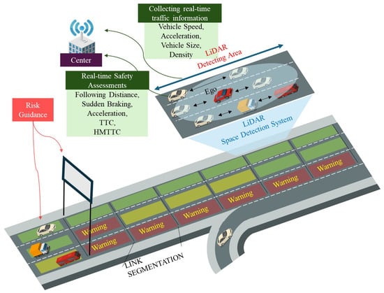
Figure 1.
Conceptual Illustration of the Proposed System.
Building upon this concept, two indicators, the Hazardous Modified Time to Collision (HMTTC) and the Searching for Safety Space (SSS), are introduced to evaluate temporal and spatial risk dynamics across varying traffic environments. The methodology adopts the aerial-based traffic flow theory introduced by Daganzo et al. [1], applying it directly to road-level LiDAR data. To validate the proposed approach, probe vehicles equipped with LiDAR were deployed on selected highway and urban segments in South Korea, capturing data under diverse conditions, including both daytime and nighttime operations. Unlike fixed-point monitoring systems, this method captures 3D spatial data dynamically from moving vehicles, providing a richer and more continuous understanding of roadway dynamics.
Following data acquisition, AI-based techniques are applied to extract relevant traffic features from the raw 3D point clouds. The processed data are analyzed to assess congestion and evaluate road safety using surrogate safety measures such as HMTTC and speed standard deviation. These metrics enable the systematic identification of high-risk areas and potential collision zones, contributing to a proactive and data-driven framework for urban traffic management.
This study presents an extended and enhanced version of our previous work [2]. Earlier research focused primarily on analyzing highway conditions using LiDAR-based probe-vehicle data to estimate surrogate safety indicators, such as TTC and MTTC. In contrast, the present study expands the scope to urban environments, incorporating additional datasets collected under various traffic and lighting conditions. Furthermore, an AI-based correlation analysis is introduced to investigate the relationship between traffic dynamics and surrogate safety indicators, thereby enhancing the interpretability of road safety assessment. All datasets were independently reprocessed to ensure data integrity and avoid overlap with the previous study.
1.1. Background
With the rapid urbanization and increasing vehicle ownership worldwide, the need for efficient traffic monitoring and management has become more critical than ever. Accurate and continuous observation of traffic conditions is essential not only for ensuring smooth mobility but also for enhancing road safety and supporting sustainable urban planning. Traditional traffic monitoring techniques have evolved from fixed, point-based detectors to multi-sensor observation systems that integrate artificial intelligence (AI) and remote sensing technologies. These advances now enable near real-time observation of traffic flow across large urban networks rather than at limited localized points.
Traffic information collection serves two major functions: safety (preventing accidents, mitigating risks) and mobility management (improving travel speed, predicting congestion, and supporting policy decisions). According to Daganzo et al. [1], methods for collecting traffic information can be categorized into three perspectives: point-based observation from the roadside, mobile-based observation from within the traffic flow, and aerial-based observation from above. Figure 2 illustrates these three representative approaches.
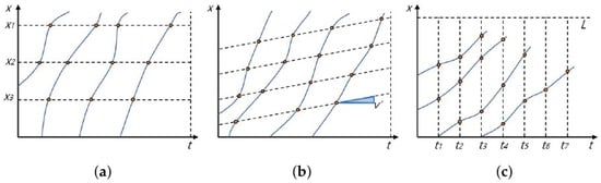
Figure 2.
Methods of collecting traffic information: (a) observing at the roadside (fixed observation point), (b) observing while moving within the traffic flow (moving observation point along the time axis), and (c) observing from the sky (time-axis movement). Yellow circles indicate the observed positions of vehicles at each time step. Blue solid lines represent the trajectory of the moving observer, and dashed lines depict the trajectories of surrounding vehicles over time.
In Figure 2, the horizontal axis (x) represents the observation point along the road, and the vertical axis (t) indicates time. Each yellow dot denotes the position of a vehicle observed at a given time step. Figure 2a depicts fixed-point observation at the roadside, where the observation position (x) is constant while time progresses vertically. Figure 2b shows mobile observation within the traffic stream, where both the observation position and time progress together. Figure 2c illustrates aerial observation from above, where observations cover multiple positions simultaneously as time advances. These conceptual diagrams describe how traffic phenomena can be monitored from different spatial and temporal perspectives.
Recent progress in AI-based remote sensing, particularly vehicle-mounted LiDAR systems, has blurred the boundaries among these categories, enabling continuous and high-resolution traffic monitoring through moving vehicles that act as mobile sensing units at the city scale.
Point-based detection methods, such as inductive loops and video cameras, have been widely used to collect data on traffic volume and spot speeds. Although these methods provide useful localized data, they are limited in capturing continuous traffic flow due to spatial discontinuity, high installation and maintenance costs, and difficulty in route-level analysis. Segment-based detection techniques, including Automatic Vehicle Identification (AVI), Roadside Equipment (RSE), Toll Collection Systems (TCSs), GPS-based probes, and mobile sensors were introduced to estimate travel times and provide broader spatial coverage [3]. However, these methods still have inherent drawbacks, such as data latency, sample bias, and reliance on user participation. Aerial-based approaches initially relied on manned aircraft and later adopted unmanned aerial vehicles (UAVs) for traffic data collection. While these systems enable wide-area monitoring, they are constrained by weather conditions, flight regulations, limited operational time, and pilot expertise requirements.
The continuous growth in vehicle density and traffic congestion has heightened the need for precise and scalable monitoring of traffic states for safety management. Conventional traffic evaluations—based on capacity analysis and Levels of Service (LOS) provide a macroscopic understanding of flow but are limited in assessing dynamic interactions between individual vehicles. Seo et al. [4,5,6] demonstrated that vehicle-mounted probe systems equipped with GPS and monocular cameras can accurately estimate hourly traffic conditions even with a small data sampling rate (0.2%), showing the potential of mobile-based sensing. Building on these advancements, the present study introduces the conceptual foundation for a LiDAR-based probe vehicle approach that integrates the advantages of aerial observation and mobile sensing. Unlike previous fixed or discrete systems, this framework enables continuous three-dimensional monitoring of road environments and provides the basis for advanced safety and traffic analysis presented in the following sections.
1.1.1. Concept of Surrogate Safety Measures
Traffic safety research has long relied on crash data to evaluate roadway risk, but such data are often sparse, delayed, and limited to recorded incidents. To overcome this limitation, the concept of Surrogate Safety Measures (SSMs) was introduced as an analytical approach that quantifies potential collision risks through observable vehicle movements. SSMs provide continuous, quantitative indicators that can predict hazardous situations before actual accidents occur, thereby supporting proactive safety management.
SSMs are typically categorized into three analytical perspectives: temporal, distance-based, and deceleration/speed-based measures. The U.S. Federal Highway Administration (FHWA) developed one of the most representative models, the Surrogate Safety Assessment Model (SSAM) [7], which evaluates vehicle conflicts using simulated trajectory data derived from microscopic traffic models. Subsequent studies have refined these measures to better reflect real-world dynamics. Mahmud et al. [8] emphasized that no single indicator can fully represent all traffic risks and highlighted the importance of multi-criteria analysis. Peng et al. [9] validated that surrogate measures based on micro-level trajectory features correlate well with actual collision probabilities, while Amini et al. [10] extended the application of SSMs to pedestrian–vehicle interactions through temporal–spatial proximity analysis.
Temporal measures, such as the Time to Collision (TTC), have become the most widely adopted indicators of SSMs. Van der Horst et al. [11] proposed a TTC threshold of 4.0 s, considering driver reaction time, while Touran et al. [12] applied Monte Carlo simulations to evaluate the safety of Autonomous Intelligent Cruise Control systems. Lee et al. [13] measured TTC and deceleration responses in rear-end collision avoidance scenarios, which account for nearly 30% of road accidents. Further simulation-based studies, such as those by Gettman and Head [14], analyzed multiple SSMs (e.g., TTC, PET, and DR) in diverse intersection environments.
In real-world applications, researchers have attempted to bridge the gap between simulation and observation. Katja et al. [15] compared theoretical and empirical TTC values at intersections, showing that TTC and headway are independent but complementary indicators. Hourdos et al. [16] applied video-based SSM detection on a Minnesota highway, achieving a 58% conflict detection rate with 6.8% false alarms. Guido et al. [17] used smartphone-based GPS trajectory data to estimate TTC and Deceleration Rate to Avoid Crash (DRAC), identifying merging sections as high-risk areas.
Overall, the existing body of work demonstrates the effectiveness of SSMs in evaluating risk, but also reveals persistent limitations. Most prior research relies on simulated or fixed observation environments, restricting their ability to capture complex, multi-lane interactions in real-world traffic. Furthermore, traditional SSM frameworks mainly focus on longitudinal risk evaluation, neglecting lateral evasive opportunities and dynamic inter-vehicle behavior. To address these gaps, the present study extends the application of SSMs by integrating LiDAR-based three-dimensional sensing and introducing a new concept called Searching for Safety Space (SSS), which considers evasive maneuverability and adjacent-lane interactions for a more comprehensive safety assessment.
1.1.2. Key Traffic Safety Evaluation Indicators and Characteristics
This section describes the primary indicators commonly used in traffic safety evaluations, along with their characteristics. These measures are instrumental in assessing the safety performance of traffic systems and critical for identifying potential risk factors that could lead to traffic incidents.
Among various surrogate safety measures, time-based indicators such as the Time to Collision (TTC) have been most widely adopted due to their simplicity and intuitive interpretation.
Hayward et al. [18] were pioneers in introducing the concept of Time to Collision (TTC), initially proposed as a tool to measure the severity of traffic collisions. TTC indicates the time remaining until a collision if two vehicles continue on their current paths and speeds. In practice, a predicted collision time shorter than a set threshold between two converging vehicles indicates an imminent collision [18]. The computation of TTC is straightforward and can be derived using the formula in Equation (1), where and denote the positional coordinates of two consecutive vehicles, and represent their velocities, and is the length of the leading vehicle. Due to its comprehensiveness and other advantages, TTC has become the most frequently used surrogate safety measure and is a standard reference in numerous studies and documents, including the final report of SSAM.
Lodinger et al. [19] investigated differences in accuracy and reaction time between manual and autonomous driving during TTC assessments. Their study demonstrated that autonomous systems are more accurate and prompt in determining TTC [19]. Jiménez et al. proposed a simplified TTC that could be applied to collision avoidance systems. They analyzed the risk of TTC collisions at intersections and other locations by considering the initial collision points of vehicles [20]. Montgomery et al. [21] personalized the timing of forward collision warning alerts by analyzing age- and gender-related behavioral differences using real driving record data from 108 participants over 1 year. Their study found a statistically significant difference, showing that men and older adults perceive risk at higher TTC levels compared to women and younger adults when braking [21].
However, conventional TTC assumes constant velocity and neglects acceleration effects, which limits its applicability in dynamic traffic conditions. To address these limitations, Ozbay et al. [22] introduced the Modified Time to Collision (MTTC), which incorporates acceleration and deceleration terms for more realistic analysis, as shown in Equation (2). In their study, micro-level simulation through PARAMICS was employed instead of intersection analysis to assess potential collision risks and their severity on link-based analyses. Furthermore, the Crash Index (CI), which factors in collision severity, and the Crash Index Density (CID), which calculates the CI for the entire segment, were introduced. The developed metrics were validated using real accident data [22].
Here, and denote the velocities of the following and leading vehicles, respectively; and represent their accelerations (negative for deceleration); D is the initial distance between the two vehicles; is the relative velocity; and is the relative acceleration.
Subsequent studies have refined and expanded TTC-based measures to improve collision prediction accuracy. Ozbay et al. [22] proposed the Modified Time to Collision (MTTC), which incorporates acceleration and deceleration to account for dynamic traffic conditions. Saffarzadeh et al. [23] later introduced the Generalized TTC (GTTC), extending the concept to encompass a broader range of vehicle interactions and motion characteristics. Minderhoud and Bovy [23] further developed two complementary indices, Time Exposed TTC (TET) and Time Integrated TTC (TIT), to evaluate both the duration and cumulative intensity of collision risk over time. TET quantifies the total time a vehicle remains below a predefined TTC threshold, whereas TIT integrates the TTC values across the observation period to express cumulative exposure to potential collision risk. Behbahani et al. [24] introduced the Comprehensive Time-based Measure (CTM), which jointly considers the magnitude and variability of TTC to improve the accuracy of collision likelihood estimation. Other variants, such as the Enhanced TTC (ETTC) [25], which incorporates lead-vehicle deceleration, and the Time to Collision with Disturbance (TTCD) [26], which accounts for slow-moving vehicles or external perturbations, further extend the applicability of time-based surrogate measures under complex traffic conditions.
Table 1 summarizes the continuous evolution of these time-based safety indicators (MTTC, GTTC, TET, TIT, CTM, ETTC, and TTCD), highlighting their respective analytical focus, strengths, and limitations. These developments collectively reflect the ongoing effort to enhance predictive accuracy, interpretability, and adaptability of surrogate safety metrics for diverse and realistic driving environments. In addition to the surrogate safety measures previously discussed, various other indices such as the Aggregated Crash Index (ACI) [27], Stopping Headway Distance (SHD) [9], and Deceleration-based Surrogate Safety Measures (DSSM) [28] continue to be proposed and refined by researchers.

Table 1.
Overview of representative time-based traffic safety measures.
In addition to the aforementioned studies, recent research has explored diverse approaches to road traffic management and analysis. Fanti et al. [30] developed a decision support system (DSS) for monitoring vehicles transporting hazardous materials, comprising modules for risk assessment, scenario simulation, and hazard prediction, which was successfully applied to Italian highways. Zhang et al. [31] introduced the Metaverse Traffic System (MTS), an integration of intelligent transportation systems (ITS) with metaverse technology. MTS emphasizes environmental perception for intelligent vehicles and incorporates a Parallel Vision for ITS (PVITS) framework that enables the construction of virtual traffic space, model learning via computational experiments, and feedback-based optimization through parallel execution. Gao et al. [32] proposed a method for estimating collision probabilities between multiple vehicles through comprehensive trajectory prediction, facilitating road risk assessment across diverse traffic scenarios.
Additionally, Das et al. [33] presented a traffic pattern analysis and optimization method based on Koopman theoretical modeling for quasi-periodic driven systems. Liao et al. [34] demonstrated safe and efficient ramp merging through simulation-based modeling of vehicle interactions under mixed traffic conditions. Wang et al. [35] proposed various simulation scenarios for next-generation intelligent transportation systems by integrating visual human-computer interaction (VHCI) into vehicle platforms. Collectively, these studies aim to enhance traffic safety and optimize network flow through data-driven methodologies, complementing the objectives of this study in developing a LiDAR-based traffic monitoring and safety analysis framework.
This paper proposes a next-generation sensing framework called the Moving Detection System (MDS), designed to overcome the inherent limitations of conventional traffic detection methods. Figure 3 illustrates traditional point-and-section detection systems. In Figure 3a, the blue boxes represent conventional point detectors embedded in the road surface, which record vehicle passage at fixed locations. These detectors provide localized traffic information, such as vehicle count or occupancy, at specific points. However, because they measure traffic only when a vehicle passes directly over the sensor, they are limited in capturing continuous flow dynamics or vehicle interactions between detection points. Figure 3a depicts conventional point detection, while Figure 3b represents section detection systems. Although these methods are effective for analyzing traffic flow in localized segments, they struggle to accurately assess extended road sections influenced by geometric variables, such as on- and off-ramps.
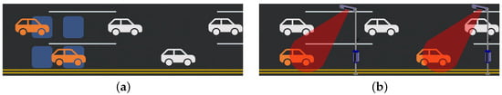
Figure 3.
Administrative-centric traffic data collection: (a) point detection, (b) section detection. Blue indicators denote point detection sensors, while red markers denote section-based measurement regions.
In contrast, as shown in Figure 4, the proposed MDS enables continuous, driver-centric detection of multiple surrounding objects while the vehicle is in motion. This approach integrates LiDAR-based sensing with environmental mapping, allowing for continuous, three-dimensional observation of dynamic road conditions. Unlike fixed or segment-based systems, the MDS provides a seamless view of spatial and temporal changes in traffic behavior, forming the foundation for the LiDAR-based safety and condition analysis framework discussed in later sections. This system aims to digitize traffic information, enabling immediate on-site safety evaluations and traffic condition monitoring through bidirectional communication.
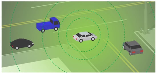
Figure 4.
Driver-centric participatory traffic data collection.
As depicted in Figure 5, the MDS approach combines the strengths of segment detection for analyzing traffic flow and section start and end points with those of aerial-based detection, enabling continuous density estimation and localized congestion recognition. In this conceptual illustration, the blue lines represent vehicle trajectories, while the red line denotes the Ego vehicle’s path equipped with a LiDAR sensor.(Pandar128, Hesai Technology, Shanghai, China). The yellow ellipses indicate the dynamic LiDAR detection zones, showing how the proposed system continuously captures vehicle motion and density information across lanes. By integrating these multi-perspective observations, MDS enables seamless spatiotemporal monitoring of traffic states along complex road geometries. One of the key advantages of the MDS method is its capability to assess variations in traffic states according to time, lane configuration, and geometric complexity. This enables detailed monitoring of lane-level traffic dynamics, an essential factor for advanced safety diagnosis and adaptive traffic management. A detailed methodological description and experimental implementation of the proposed MDS are presented in the subsequent sections.
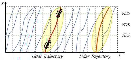
Figure 5.
Comparison of the moving detection system installation with traditional detection methods. The green dashed line represents the location of the VDS point detector, the red line shows the trajectory of the probe (Ego) vehicle, and the blue lines indicate the trajectories of surrounding vehicles. The yellow regions illustrate the probe vehicle’s dynamic detection range for identifying adjacent vehicles.
2. Materials and Methods
2.1. Materials
The materials used in this work include LiDAR-based point cloud measurements collected using a Pandar128 LiDAR sensor (Hesai Technology, Shanghai, China) and object-level information derived from them. To prepare these materials for analysis, the Ego vehicle processes raw LiDAR scans through a perception pipeline that includes PCD extraction, BEV transformation, and deep learning–based object detection. The following subsections describe how these materials are obtained.
2.1.1. Extraction of Point Cloud Data (PCD) from Driving Records
This section describes the data collection process for the probe vehicle. Before detecting adjacent objects in the driving data of the exploration vehicle, Point Cloud Data (PCD) is extracted. LiDAR sensors typically have a detection range exceeding 200 m, but the detection rate decreases with distance, which can lead to false positives. To prevent this, the detection range for adjacent objects is limited to 50 m. Additionally, PCD files are generally larger than 2D images, requiring high-performance computational resources. In this study, by limiting the range, we reduce unnecessary data and positional information, allowing for efficient extraction of the necessary data. Consequently, we propose a system that sets a Region of Interest (ROI) of 50 m to analyze road conditions. Subsequent processes involve converting the PCD into a Birds Eye View (BEV) map and performing 3D object detection for traffic analysis. These processes will be explained in detail in the following sections.
2.1.2. Vehicle Object Detection
We utilize the Point Cloud Data (PCD) extracted in the previous section to detect objects within a 3D space. While many prior studies have explored image-based object detection in transportation environments [36,37], this work extends such approaches by employing LiDAR data, which provides more robust 3D perception and can be further enhanced through future sensor-fusion techniques. For object detection, this paper employs the Voxel-RCNN (official implementation) [38] PointRCNN, SECOND, CenterPoint, and TransFusion were only mentioned for comparison purposes and were not used in our experiments. Thus, version/source information is not required. to identify vehicles driving near the Ego vehicle. Voxel-RCNN is an outstanding 3D object detection framework that introduces an innovative approach for efficiently processing point clouds in autonomous driving applications. The core of Voxel-RCNN lies in its ability to effectively integrate voxel-based feature extraction with Region Proposal Networks (RPNs), thereby enhancing both the accuracy and efficiency of 3D object detection. Compared to other detectors such as PointRCNN [3], SECOND [39], it achieves a superior balance between detection accuracy and inference speed, making it suitable for real-time LiDAR perception. In this study, the use of Voxel-RCNN is primarily from an implementation perspective to validate the feasibility of the proposed LiDAR-based monitoring framework, rather than to emphasize a specific model architecture. Nevertheless, the proposed framework is model-agnostic and can flexibly incorporate more recent architectures, such as CenterPoint [39] or TransFusion [40], to further enhance detection performance in future work.
Detected results allow for the simultaneous acquisition of vehicle height and length data for vehicles moving around the Ego vehicle. This data, difficult to collect with traditional sensors, serves as foundational material for future density and safety evaluations. Three-dimensional LiDAR data is utilized for deep learning-based object detection. After detecting objects with LiDAR sensors, the process does not use the z-value of the PCD to optimize computation, converting it into a two-dimensional BEV map. This conversion from the world coordinate system to the commonly used two-dimensional xy coordinates is primarily for the efficient use of large volumes of 3D big data in real-time operations. Reducing the data to two dimensions decreases computational load, enhancing process efficiency and enabling intuitive visualization in an analyzable 2D map format. This visualization aids intuitive understanding of the progression and appropriateness of operations, enabling direct analysis of road conditions. The system maps lane information for traffic analysis by lane, using GPS data to capture the road’s lane layout. It employs a LiDAR-based lane recognition method for mapping lane information. LiDAR sensors can identify reflectivity, enabling the extraction of lane features. To determine the lane-marking distribution used for lane-level traffic analysis, this study adopts a hybrid method that combines GPS-referenced lane geometry with LiDAR-based lane detection. Lane-marking features were extracted from the LiDAR point cloud using an intensity-based filtering and clustering approach, following the lane detection methodology proposed by Choi et al. [41]. This method enables reliable identification of lane markings even under partial occlusions or lane-wear conditions. The LiDAR-derived lane features were then aligned with GPS-based road geometry to construct a stable lane-distribution map, which forms the basis of the lane boundaries used in the analysis.
This hybrid lane model allows the accurate assignment of detected vehicles to their corresponding lanes during SSS and traffic-state analysis. Following the conversion to two dimensions for object detection and visualization, and lane recognition, the detected vehicle data is output in a tabular format, making it suitable for use as traffic data. These results provide foundational data for processing individual and surrounding vehicle speeds, spacing, and other traffic information.
2.2. Methods
In this section, we describe the methods used for continuous traffic-condition monitoring and safety evaluation using the processed traffic information, including density, speed, and surrogate safety measures (SSMs). Furthermore, we propose an improved safety evaluation framework based on HMTTC and the concept of evasive safety space (SSS).
2.2.1. Methods for Tracking Moving Objects and Calculating Speed
Tracking IDs are assigned to detected vehicles to maintain their identities across frames and to extract speed-related information. Tracking methods are generally categorized into point tracking, kernel tracking, and silhouette tracking For vehicle tracking, this study employs the Intersection over Union (IoU) metric, a widely used and reliable measure in computer vision. IoU determines whether a detected object corresponds to the same vehicle across consecutive frames based on the overlap ratio, requiring a predefined threshold. To adapt IoU to dynamic traffic environments, we define a context-dependent IoU threshold, referred to as the Contextual Intersection over Union (CIoU), which dynamically adjusts according to vehicle length and relative speed. This formulation allows the threshold to reflect real-world variations in vehicle size and motion, enhancing robustness under heterogeneous traffic conditions.
The CIoU threshold used in this study is computed as follows:
Here, represents vehicle length, denotes the relative speed between two vehicles (converted using 3.6 from km/h to m/s), and t is the unit time. During temporary occlusions or limited field of view, the system preserves a vehicle’s tracking ID for 2–3 frames using its last known position and velocity vector. If the object reappears and satisfies the CIoU threshold with the predicted position, the same ID is retained; otherwise, a new ID is assigned. This strategy ensures stable tracking performance even under intermittent visibility.
Because the tracking ID is preserved temporarily, this process inherently performs short-term motion prediction and suppresses abrupt bounding-box shifts. As a result, brief occlusions do not propagate into large speed or acceleration errors, since kinematic estimates are aggregated over multiple frames.
According to Wakasugi et al. [42], the speed difference between the driving lane and the overtaking lane on a four-lane highway is typically less than 30 km/h based on a cumulative 90% criterion. In contrast, this study adopts a more conservative setting by defining using the maximum observed difference between highway speed limits (120 km/h) and minimum speeds in congested flow (50 km/h), resulting in km/h. The vehicle length is defined using the average length of a passenger car (4.4–4.6 m), which produces CIoU values ranging from 0.69 to 0.70. Accordingly, the IoU threshold is set to 0.7 in this study.
It is also important to note that for larger vehicles such as buses and heavy trucks, the average vehicle length is significantly greater than that of passenger cars. Because the CIoU formulation directly increases with vehicle length, long vehicles (typically 10–12 m or more) naturally produce CIoU values exceeding 0.7 under the same and t conditions. Therefore, applying the passenger-car-based threshold of 0.7 does not disadvantage large vehicles; rather, they satisfy the threshold more easily due to their greater longitudinal dimensions. Thus, the chosen CIoU threshold of 0.7 remains valid and robust across different vehicle types.
For vehicles identified as the same entity across frames, their speeds are estimated relative to the Ego vehicle, which provides the only directly measurable speed information. As shown in Figure 6, the position of each detected vehicle is tracked over consecutive frames using its assigned tracking ID. Based on these tracked positions, the relative speed of surrounding vehicles is computed using the following relation:
where denotes the longitudinal displacement of the surrounding vehicle over the interval , and represents the relative speed between the Ego vehicle and the detected vehicle. This displacement-based velocity estimation process enables the computation of individual vehicle speeds, as illustrated in Figure 7, providing essential traffic information for subsequent analyses.
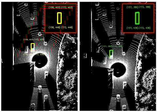
Figure 6.
Identification and Assignment of Tracking IDs for Moving Vehicles. Yellow boxes indicate objects detected in the previous frame, green boxes represent objects detected in the current frame, and the red box highlights the zoomed-in region for detailed visualization.
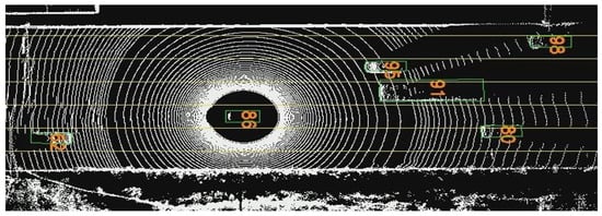
Figure 7.
Calculation results of individual speeds in driving spaces. The yellow line denotes the detected lane boundary, the numbers indicate the estimated speeds of individual vehicles, and the green boxes represent the detected vehicle objects.
The LiDAR-based object extraction framework enables the collection of a wide range of traffic information in moving sections. Although all potential variables are summarized in Table 2, this study focuses specifically on speed, acceleration, and density, which serve as the foundation for traffic condition monitoring and safety assessment. The next section describes how these processed data are used to develop continuous monitoring methods for evaluating traffic conditions and surrogate safety indicators, forming the analytical basis for urban traffic risk assessment.
Table 2.
Data collection and description.
2.2.2. Traffic Condition Monitoring Methods
Traffic condition monitoring utilizes individual vehicle information to continuously assess traffic conditions using key performance indicators such as density and speed. The occupancy rate (similar to density) in a driving section refers to the proportion of space occupied by vehicles on the entire road. It is calculated by dividing the space occupied by vehicles by the total lane area, providing a more detailed assessment of road conditions than traditional density measures (vehicles/km). Lane-specific analysis can effectively evaluate conditions at highway entrances and exits at an early stage. Additionally, calculating occupancy rates using LiDAR-based road condition data enables a more accurate assessment of road conditions at the section level by determining vehicle length, offering advantages over traditional vehicle-count-based density measures.
In this paper, we perform a safety evaluation defined as a surrogate safety measure by extracting vehicle data such as direction, speed, and acceleration using the unique tracking IDs for individual vehicles described in the previous section. The extracted data, as summarized in Table 2, are utilized to calculate the road safety margin based on the Time-to-Collision (TTC) concept. The TTC, originally introduced by Hayward [18], has been widely adopted as a surrogate safety indicator to quantify the time remaining before a potential collision between two vehicles.
Subsequent studies by Minderhoud and Bovy [23] and Ozbay et al. [22] enhanced the TTC model by incorporating acceleration and driver reaction components to improve predictive accuracy under dynamic driving conditions. This approach, referred to as the Modified Time to Collision (MTTC), extends the conventional TTC to account for variations in acceleration and vehicle interactions. Building upon this concept, our study defines the Hazardous Modified Time to Collision (HMTTC), which emphasizes critical conditions where MTTC values fall below three seconds, thereby enhancing the applicability of surrogate safety evaluation for real-world urban traffic scenarios. The frequency of HMTTC occurrences is employed as an indicator of road stability in conjunction with lane-level density analysis.
2.2.3. Searching for Safety Space (SSS)
In this paper, we introduce the concept of Searching for Safety Space (SSS), which enables analysis of situations in which a driver facing potential danger can either brake or perform an evasive steering maneuver depending on the available space in adjacent lanes. Traditional safety space models primarily consider only the vehicles directly ahead and behind, neglecting lateral interactions due to the limited field data available from traditional observation methods. By utilizing LiDAR sensors, this study overcomes these constraints by analyzing interactions with all surrounding vehicles within approximately a 50 m radius of the Ego vehicle. As shown in Figure 8, the Ego vehicle (white) continuously monitors the surrounding environment to identify leading vehicles (orange and green) and following vehicles (blue) in both adjacent lanes. The variables through represent the longitudinal distances between the Ego and neighboring vehicles, while denotes the lateral entry angle during a potential lane change, and MTTC represents the Modified Time to Collision with the forward vehicle. The yellow-shaded regions indicate the dynamically available safety spaces for evasive maneuvers, reflecting the areas where the Ego vehicle can safely change lanes or decelerate based on its current speed and acceleration. Previous studies have shown that lane-change entry angles typically range between 5° and 7°, and the resulting increase in travel distance is negligible, validating the practicality of the proposed SSS model for safety assessment. It should also be noted that the assumed lane-change entry angle of 5°–7° reflects typical voluntary lane-change behavior observed on motorways. Therefore, the proposed SSS formulation is intended for normal lane-change situations and does not model aggressive or emergency evasive steering maneuvers, where much larger entry angles and rapid lateral dynamics may occur. As this study focuses on presenting a conceptual LiDAR-based framework for lane-level safety assessment, extending the SSS model to cover emergency avoidance scenarios, remains an important direction for future research. In addition, the SSS formulation relies on a linearised kinematic approximation in which the longitudinal motion during a short prediction interval is represented using a constant-velocity relation and the lateral trajectory is simplified to a fixed entry angle. Such assumptions are suitable for normal lane-change behavior where acceleration varies smoothly, and lateral motion remains limited, but they do not fully represent nonlinear vehicle dynamics that may arise during rapid braking, abrupt steering inputs, or emergency obstacle-avoidance maneuvers. These simplifications and their implications for extreme scenarios have now been explicitly discussed as limitations of the proposed framework.
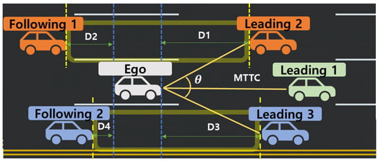
Figure 8.
Conceptual diagram of the search for safety space. Yellow solid lines indicate the potential evasive paths of the Ego vehicle, yellow dashed lines represent directional boundaries used in safety-space estimation, and blue dashed lines denote lane boundaries. The distances , , , and indicate the relative spacing between the Ego vehicle and surrounding leading or following vehicles in each direction.
Figure 9 illustrates the process of determining collision presence based on lane-changing (evasive steering) actions. In this system, the potential for collision avoidance is assessed by calculating collision presence, thereby identifying safe spaces for evasion. Figure 9a depicts the initial moment, while Figure 9b showcases the anticipated moment of collision. represents the vehicle ahead in the target lane (Leading 2), is the distance between the Ego vehicle and the vehicle ahead in the target lane (), is the distance traveled by within a time interval of t seconds, and is the distance traveled by the Ego vehicle within the same time interval. The term represents the horizontal distance between the Ego vehicle and following the lane change. For a collision to occur (as shown in case Figure 9b), the condition must be met. Consequently, the equations for assessing the availability of safe spaces in all directions are given in Equations (5)–(8).
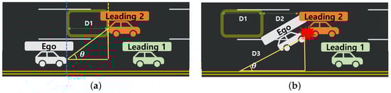
Figure 9.
Determining Collision Probability (Time) Based on Lane Change maneuvers. (a) Illustration of the anticipated collision moment, showing the steering angle and the spatial relationship with the leading vehicle. Distance represents the initial spacing used in collision assessment. Blue dashed lines denote lane boundaries, while yellow dashed lines indicate directional reference lines used in the collision-detection calculation. (b) Illustration of the collision condition where the Ego vehicle approaches a leading vehicle in the adjacent lane. Distances , , and represent the relative spacing and movement of the Ego and leading vehicles used in the collision assessment.
Equations (5) and (6) describe the formulas for determining the availability of safe space in the left lane. Equation (5) represents the decision formula for assessing the possible evasion space with the vehicle in front in the left lane, while Equation (6) pertains to the evaluation of the possible evasion space with the vehicle behind in the left lane. Equations (7) and (8) continue this theme for the right lane. Equation (7) is concerned with evaluating the possible evasion space with the vehicle in front in the right lane, and Equation (8) deals with the assessment of the possible evasion space with the vehicle behind in the right lane. Here, V denotes vehicle speed, a represents vehicle acceleration, t represents unit time, D indicates the distance between vehicles, and symbolizes the steering angle.
To prevent numerical instability when certain terms in the SSS and MTTC formulations approach zero, particularly the relative speed in the denominator, the implementation applies a numerical protection mechanism. A small positive constant is added to the denominator, or threshold-based handling is used for near-zero values. These measures ensure stable computation while preserving the theoretical structure of the original kinematic model.
To clarify the probabilistic interpretation of the proposed method, the collision time x derived from Equations (9)–(14) is used to define the collision probability . The collision probability is calculated as the ratio of time intervals where (i.e., hazardous conditions) to the total observation period, as expressed below:
This probabilistic metric represents the likelihood of a collision occurring within a given observation window and allows for quantitative comparison across different traffic scenarios. The derivation of Equations (9)–(14) is based on several simplifying assumptions: (1) both the Ego vehicle and surrounding vehicles maintain constant acceleration within the observation window t; (2) driver reaction time and steering delay are neglected; (3) the steering angle is assumed to remain within 5°–7°, allowing the use of the cosine approximation; and (4) environmental factors such as weather, road slope, and friction are not explicitly modeled. These assumptions enable a tractable analytical formulation while maintaining practical validity for LiDAR-based sensing environments.
This paper proposes a method to improve stability assessment through the verification of secured safe spaces. The proposed safety assessment method consists of two main stages: (i) calculating the HMTTC with the preceding vehicle, and (ii) evaluating the availability of SSS by calculating the HMTTC with vehicles ahead and behind in adjacent lanes. The calculation of HMTTC and the assessment of overtaking possibilities are conducted for all vehicles within the Ego vehicle’s sensing range, with individual calculations based on real data for each vehicle.
The proposed improvement to stability evaluation by assessing safe space availability based on HMTTC is feasible. Initially, let x represent the time until a collision occurs with the preceding vehicle at t; the relationship between the two vehicles can be expressed through Equations (9) and (10). Equation (10) reformulates Equation (9) into a quadratic equation. Here, denotes the acceleration of the leading vehicle at time t, represents the acceleration of the Ego vehicle at time t, is the speed of the leading vehicle at time t, is the speed of the Ego vehicle at time t, is the angle of the leading vehicle from the direction of the Ego vehicle’s front, and d signifies the distance between the Ego vehicle and the leading vehicle. By substituting the conditions of the Ego vehicle and the vehicles ahead and behind into Equation (10), the expected collision time x can be calculated. The formula can be simplified based on acceleration and the distance between vehicles. In cases where acceleration is equal, such as , it simplifies to Equation (11), and in cases where accelerations differ, as in , it is consolidated to Equation (12).
All derivations from Equations (9)–(14) are conducted under the simplifying assumptions stated earlier. These ensure analytical tractability while retaining physical validity for LiDAR-based scenarios.
When organizing the formulas based on the distance between vehicles, denoted as D, we find that in situations where there is a discernible distance between the vehicles, i.e., when , the formula can be consolidated as shown in Equation (13). Furthermore, this allows for the determination of the range of x, which can be calculated as illustrated in Equation (14). This approach emphasizes the significance of vehicle spacing in predicting collision times and enhances the precision of the safety evaluation model by incorporating the spatial dynamics between vehicles.
To visualize the results obtained from the collision time determination process, the Ego vehicle is represented as a moving rectangular box divided into four sections, as shown in Figure 10. Color coding is used to indicate different safety conditions: green represents a normal condition where the MTTC critical time exceeds 4.5 s; orange indicates a potential risk condition where it is between 3 and 4.5 s; and red denotes an unavoidable collision condition where it falls below 3 s. This continuous visualization of evasive space availability enables intuitive monitoring and assessment of road safety conditions. A detailed explanation of the experimental procedures for the proposed methodology is provided in the following section.
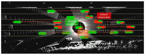
Figure 10.
Calculation results of modified TTC and Searching for Safety Space (SSS).
Through the application of the equations and safety-space analysis described above, the following section presents the experimental implementation and evaluation results to validate the proposed HMTTC- and SSS-based safety assessment framework. It should also be noted that the present study focuses on the conceptual design and feasibility verification of the proposed LiDAR-based traffic monitoring framework rather than its full-scale implementation. The experiments were conducted on various highway environments in Korea, covering both daytime and nighttime conditions and diverse road geometries, including straight and curved segments. However, adverse weather conditions such as heavy rain or fog, which can significantly affect LiDAR sensing performance, were excluded from the experimental scope. In future work, this framework can be extended by integrating more robust sensing modalities such as 4D Radar to ensure reliable operation under adverse weather conditions.
In addition, this study adopts LiDAR as the primary sensing modality due to its ability to provide high-resolution 3D geometric information for efficient traffic monitoring. The accumulated point clouds generated by LiDAR can also be used to update high-definition (HD) maps, not merely as static maps but as dynamic layers incorporating real-time traffic information. Although LiDAR exhibits limitations under adverse weather, these issues can be mitigated through future integration of more robust sensing modalities, such as 4D Radar.
3. Results
In this section, we evaluate the proposed LiDAR-based road-condition monitoring framework using field data collected on Korean highways. Korean road environments are highly diverse and complex due to the dense concentration of highways and urban expressways, especially in metropolitan areas. Traffic conditions vary significantly between daytime and nighttime, reflecting differences in congestion levels and illumination conditions. Additionally, features such as exclusive bus lanes, on- and off-ramps, and frequent lane merges create a dynamic traffic environment that requires lane-specific rather than section-averaged analysis. Therefore, the experimental dataset in this study was collected to represent these varied and realistic driving conditions on Korean highways. LiDAR-equipped vehicles recorded data across multiple representative segments, including uncongested morning sections, peak-hour congestion zones, and signalized intersections, with each experiment conducted over an hourly driving session to capture temporal variations in traffic flow. The LiDAR detection range was set to 50 m, balancing sensing reliability and computational efficiency within the practical limits of point cloud density and signal return strength. As reported by Corral-Soto et al. [43], LiDAR detection accuracy decreases at longer distances due to the reduction in point cloud density and weaker reflected signals. Peri et al. [44] further demonstrated that restricting the effective detection range is essential to maintain an optimal balance between detection accuracy and latency in 3D perception systems. In addition, Khoche et al. [45] noted that object detection reliability beyond 50–60 m sharply declines due to increased point sparsity and diminished return intensity, emphasizing the practical limitations of current LiDAR sensors for long-range detection. Accordingly, the 50 m range adopted in this study represents a reasonable and empirically supported threshold for ensuring reliable performance in lane-level traffic monitoring. Furthermore, because this study employs a probe-vehicle–based monitoring approach, the meaningful interactions with surrounding traffic occur well within this 50 m range. Extending the ROI beyond this distance would not provide additional analytical benefit for lane-level traffic and safety assessment, while relying on LiDAR measurements that are inherently less reliable at longer ranges. Therefore, the 50 m ROI used in this study is both practically sufficient and methodologically appropriate for the intended traffic-monitoring framework. Based on these conditions, this section evaluates the proposed methodology using situational road data from Korea to validate the system’s approach.
As seen in prior studies, the TTC threshold commonly ranges from 1 to 4 s, with several different standard values used in the literature. To determine which threshold is appropriate for this study, we examined Korean legal criteria, international cases, and our field-collected data. Oh et al. [46] adopted a TTC threshold of 3 s, as established in earlier research, for rear-end collision risk analysis. Their experiment was conducted over a 15 min period on a section of a domestic highway, with the analysis range limited to 70 m. Table 3 summarizes the hourly TTC distribution from their study. The results indicated that TTC values below 3 s accounted for approximately 10% in lane 1, 8% in lane 2, and 7.5% in lane 3. As illustrated in Figure 11, observations with TTC under 3 s comprised about 9% of all cases in total [46].
Table 3.
Hourly distribution of lane-specific TTC by Oh et al. [46].

Figure 11.
Cumulative graph of lane-specific TTC distribution by Oh et al. [46].
Based on data collected in the field and employing the cumulative distribution method used by Oh et al. [46], we analyzed the MTTC cumulative distribution results for two sections of Korean highways: the Pangyo–Osan and Pangyo–Seocho sections. The analysis of MTTC occurrences, as illustrated in Table 4 and Figure 12, revealed that the cumulative percentage of MTTC occurrences under 3 s was approximately 1% for the Kyungbu Expressway’s Busan direction, specifically the Pangyo–Osan section. In contrast, the Pangyo–Seocho section, which often experiences congestion in the direction towards Seoul, showed a cumulative distribution of MTTC at about 4%. Taken together, these analyses justify the choice of 3 s as the HMTTC threshold in the remainder of this study.
Table 4.
Our hourly distribution of lane-specific TTC.
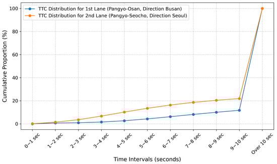
Figure 12.
Our cumulative graph of lane-specific TTC distribution.
Additionally, using field data from the Kyungbu Expressway in the Busan direction, specifically the Pangyo–Osan section, we compared the number of MTTC occurrences across different threshold values. The results, as depicted in Figure 13, indicate that while occurrences with a 1-s threshold are very rare, appearing at most twice at the same moment, the occurrences increase to a maximum of 6 cases for a 3-s threshold and up to 9 cases for a 4.5-s threshold. This pattern, showing an appropriate increase in MTTC at change areas such as IC entrances and exits, and a decrease in other sections, is considered an adequate indicator of safety assessment results. The threshold that best demonstrates this trend, based on field comparison results, was determined to be 3 s. Thus, we conclude that a 3-s threshold serves as an appropriate safety surrogate, suitably representing accident risk, and have opted to use it in our analysis. MTTC occurrences of less than 3 s are referred to as HMTTC in this study.
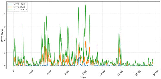
Figure 13.
Graph of MTTC incidents.
In this section, we conducted experiments centered around the evaluation of traffic safety using a variety of traffic information collected from LiDAR sensors during field surveys, in order to validate the proposed methodology. Detailed explanations will be provided in the subsequent sections.
Comparison of Lane-Specific Speeds and Overall Average Speed
In this section, we have analyzed the comparison between lane-specific speeds and the overall average speed of a segment based on data collected from the field. Generally, traditional traffic information detection methods use the concept of an average speed across the entire space, which has limitations in providing accurate information in situations of traffic flow changes, such as congestion. In this study, lane-specific speeds were derived by calculating the relative velocity of each vehicle with respect to the Ego vehicle using Equation (4), and then averaging these relative velocities for all detected vehicles within each lane. As illustrated in Figure 14a, utilizing LiDAR data allows for the immediate comparison of speed differences between lanes. Excluding the first lane (blue), which is a bus lane, there’s a noticeable speed difference of approximately 30 km/h between the second lane (orange) and the fifth lane (purple), indicating that congestion in the fifth lane also affects the fourth lane (red). In the case of Figure 14b, we examined lane-specific speeds and the overall segment-average speed in a section where congestion was gradually clearing. After the congested section, a sharp increase in speed was observed, indicating a similar pattern of increase in the average speed. However, differences in speed between lanes were still evident, contributing to discrepancies in navigation traffic information. To mitigate this, comprehensive information provision, including continuous collection of lane-specific data, is necessary, for which the introduction of the MDS approach is essential.
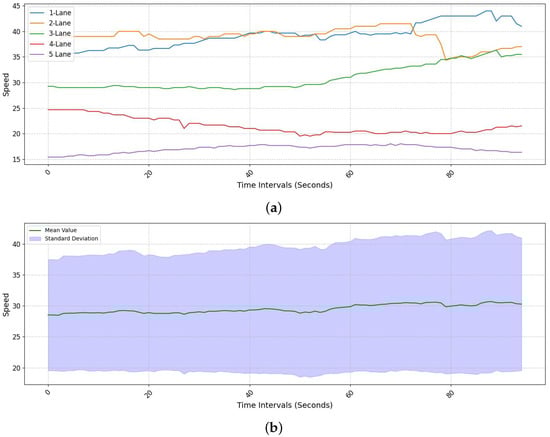
Figure 14.
Comparison of lane-specific speeds and average speed across the entire section during congestion. (a) Lane-specific speeds calculated using LiDAR-derived relative velocities, showing distinct speed differences among lanes during congested conditions. (b) Overall average speed of the road segment and the corresponding standard deviation bands, illustrating how variability across individual lanes influences the aggregated average speed.
Figure 15 illustrates the average speeds between Pangyo IC and Banpo IC, clearly showing the onset of congestion just before Yangjae IC (along the x-axis from 10 to 60). Figure 15a presents the individual speed calculations for each lane, where all lanes except the bus-only lane show generally similar speed values. In Figure 15b, the green line represents the average speed from Figure 15a, while the purple area (standard deviation 1) indicates the standard deviation including the bus-only lane, and the pink area (standard deviation 2) represents the standard deviation excluding the bus-only lane. This figure clearly illustrates how variations in individual lane speeds affect the overall average value. In particular, when the deviation in one lane is excessively large, the overall average speed fails to accurately reflect the actual traffic conditions. Through this experimental result, it was confirmed that using only the overall average speed across all lanes provides limited insight into detailed roadway conditions. The bus-only lane (Lane 1) maintains relatively stable speed fluctuations, whereas other lanes show noticeable decreases in speed near entry and exit ramps, reflecting subtle variations in traffic flow depending on the road environment. Therefore, the conventional approach that relies solely on the average speed across all lanes, including bus lanes and entry/exit lanes, is insufficient for fine-grained road condition analysis.
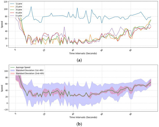
Figure 15.
LiDAR speed graph for all lanes (Pangyo to Banpo). (a) Lane-specific speeds computed from LiDAR measurements, showing variations in speed profiles across lanes. (b) Overall average speed with standard deviation bands, illustrating how lane-to-lane variability influences aggregated traffic conditions.
Figure 16 illustrates the density variation using field data for the section from Pangyo IC to Osan IC on the Busan-bound direction of the Gyeongbu Expressway. In contrast, for the Seoul-bound section from Pangyo to Banpo, initial continuous congestion was observed. Figure 16a displays the overall density changes for each lane. The first lane, being a bus-only lane, shows a significantly lower density, while lanes two through four exhibit a density pattern similar to the overall average. Figure 16b presents the density values for the fifth lane. This lane, serving as an exit and entrance lane, includes junction points at positions 40 and 80 on the x-axis, where an increase in density can be noted. The proposed method of extracting lane-specific density enables detailed analysis of changing traffic conditions at exits and entrances, thus facilitating a fine-grained analysis of expressways that include these features.
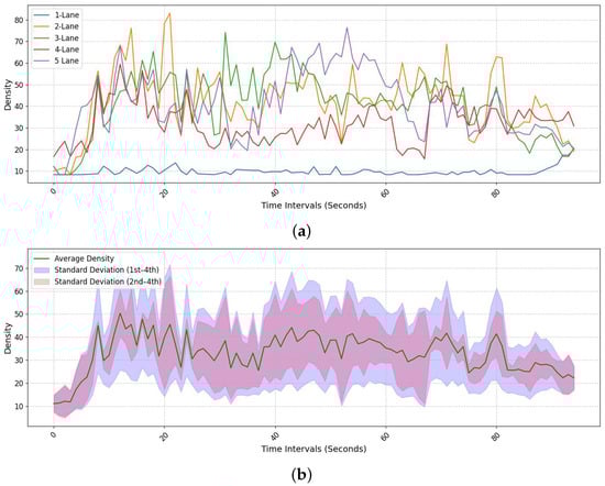
Figure 16.
Density variation graph by lane (Pangyo to Osan). (a) Density changes for lanes 1 through 5, illustrating distinct congestion patterns across individual lanes. (b) Overall average density with standard deviation bands, showing how variability among lanes influences the aggregated density profile.
The following Figure 17 compares traffic conditions between two regions using lane density and LiDAR-derived speed. In this experiment, density denotes the lane length occupied by vehicles within a 50 m window, and speed denotes the lane-average speed. Density values are plotted in blue, and LiDAR speeds in green. Figure 17a shows the segment from Pangyo IC to Osan IC, and Figure 17b from Pangyo IC to Banpo IC. Both plots visibly exhibit an inverse relationship between density and speed, consistent with the fundamental expectation that higher lane occupancy yields lower individual vehicle speeds. This visual experiment demonstrates the qualitative correlation between lane density and speed. To complement this visual evidence, subsequent experiments perform a quantitative correlation analysis between HMTTC occurrences and lane-level speed/density, thereby substantiating the proposed framework’s ability to capture congestion-related safety risk. Therefore, the method proposed in this paper can effectively analyze lane-by-lane traffic conditions.
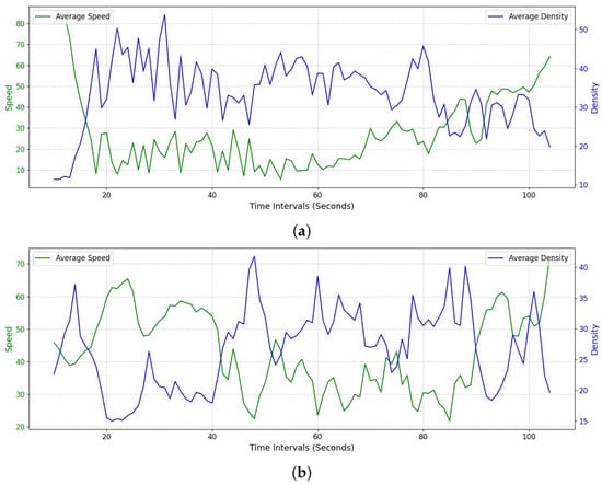
Figure 17.
Density values and LiDAR speed comparison. (a) Density and lane-average LiDAR speed for the Pangyo–Osan IC section, showing clear inverse variation between density and speed. (b) Density and lane-average LiDAR speed for the Pangyo–Banpo IC section, where persistent congestion produces different fluctuation patterns compared with the Busan-bound segment.
In this study, we assessed highway safety for the purpose of monitoring. To diagnose highway safety, we analyzed the occurrence of the surrogate safety measure, HMTTC. Figure 18a compares safety across locations by the number of HMTTC occurrences on the Pangyo–Osan IC section of the Gyeongbu Line toward Busan. The results indicate frequent HMTTC occurrences around the junction near the x-axis at 100 and the IC area near the x-axis at 300. However, it is difficult to identify specific causes or risk mechanisms from this plot alone. Figure 18b shows the Pangyo–Banpo IC section toward Seoul, a regularly congested corridor, where there is no marked increase in HMTTC occurrences around ICs or other locations. To guide interpretation, Figure 18 should be read as a hotspot map: The x-axis is the cumulative distance along each study segment (m), and the y-axis is the HMTTC count per 50 m spatial bin. This step localizes where risk symptoms concentrate but does not by itself explain the underlying causes.
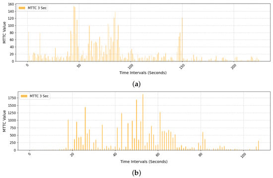
Figure 18.
Results of extracting the number of HMTTC occurrences. (a) HMTTC occurrences along the Pangyo–Osan IC section, showing concentrated risk near major junctions. (b) HMTTC occurrences along the Pangyo–Banpo IC section, where recurrent congestion does not produce localized spikes around IC areas.
In the previous analysis, it was challenging to conduct a precise safety assessment based solely on the number of HMTTC occurrences. Therefore, we additionally considered speed and density. Figure 19a compares changes in density and the number of HMTTC occurrences using field data for the Pangyo–Osan IC section toward Busan. As shown, there is a general trend in which an increase in density corresponds to an increase in HMTTC occurrences. Figure 19b shows a similar pattern in another segment. Through this experiment, we confirmed a clear association between road density and HMTTC. For Figure 19, density (right y-axis) is computed as the occupied length within each 50 m window (m per 50 m), and HMTTC (left y-axis) is the event count in the same co-registered bins. The co-movement of the two series around ramp influence areas indicates that higher density is accompanied by higher HMTTC counts, linking congestion build-up to elevated surrogate risk.
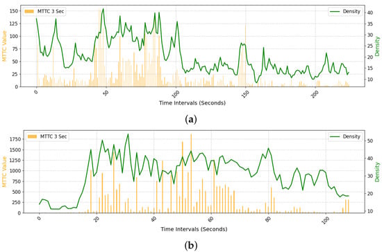
Figure 19.
Comparison of density and the number of HMTTC occurrences. (a) Density and HMTTC counts for the Pangyo–Osan IC section, showing that higher lane density generally corresponds to a greater number of HMTTC occurrences. (b) Density and HMTTC counts for the Pangyo–Banpo IC section, exhibiting a similar trend and reinforcing the relationship between congestion build-up and increased surrogate safety risk.
Figure 20 completes the picture by pairing HMTTC counts with the average speed per 50 m bin (km/h), derived from tracking-based relative velocity estimation. The inverse relationship, with lower speeds coinciding with higher HMTTC counts, is consistent across both the Pangyo–Osan and Pangyo–Banpo segments, reinforcing the link between congestion and surrogate risk.
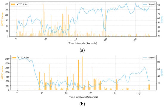
Figure 20.
Comparison of LiDAR speed and the number of HMTTC occurrences. (a) Lane-average speed and HMTTC counts for the Pangyo–Osan IC section, illustrating an inverse relationship in which lower speeds tend to coincide with higher HMTTC occurrences. (b) Lane-average speed and HMTTC counts for the Pangyo–Banpo IC section, showing consistent inverse correlation and further supporting the link between congestion and elevated surrogate safety risk.
In summary, we adopt a three-step reading: (i) locate HMTTC hotspots (Figure 18); (ii) verify that hotspots grow with density (Figure 19); and (iii) confirm the complementary inverse relation with speed (Figure 20). This staged analysis shows that HMTTC is not merely a count map but a congestion-sensitive safety indicator that reflects lane-level operational conditions. These trends are observed consistently in both the Pangyo–Osan and Pangyo–Banpo segments.
In this study, the Hazardous Modified Time to Collision (HMTTC) is treated as a surrogate indicator of collision risk that is expected to covary with macroscopic traffic states such as speed and density. To examine these relationships, we conducted a Pearson correlation analysis between HMTTC counts and lane-level averages of speed and density computed over co-registered 50 m spatial bins. In this experiment, we employed Pearson correlation to analyze the relationship among the proposed HMTTC evaluation metric, average speed, and density. The Pearson correlation coefficient [47,48] is a statistical measure used to evaluate the linear correlation between two variables. The coefficient ranges from +1 to −1, where +1 indicates a perfect positive linear correlation, 0 indicates no linear correlation, and −1 indicates a perfect negative linear correlation. The formula for calculating the Pearson correlation coefficient is given in Equation (15). In Equation (15), and represent individual sample points, while and denote the means of the X and Y samples, respectively. Equation (15) can be further expressed as Equation (16), where n is the number of data points. Along with the Pearson correlation coefficient, the p-value is often provided to evaluate the statistical significance of the correlation. The p-value indicates the probability that the observed correlation occurred by chance and is calculated using the t statistic of the Pearson correlation coefficient, as shown in Equation (17). Applying these definitions, we computed pairwise correlations for the experiments illustrated in Figure 19 and Figure 20 and summarized the resulting coefficients and p-values in Table 5. This quantifies how increases in density and decreases in speed align with elevated HMTTC occurrences, thereby linking congestion conditions to surrogate safety risk.
Table 5.
Pearson correlation coefficients and p-values.
For Figure 19, we report the correlations between HMTTC counts and density for the two study segments: and , with in both cases, indicating statistically significant moderate associations. Here, density is defined as the free-space length within each 50 m bin (larger values imply lower occupancy), which explains the negative sign: as free space decreases (i.e., effective occupancy rises), HMTTC events increase. For Figure 20, the correlations are and with , reflecting statistically significant moderate associations between HMTTC and congestion level. For the correlation calculation, we use the inverse of average speed (a congestion index) per 50 m bin, so higher index values (lower speeds) coincide with more HMTTC events, yielding positive coefficients.
Across all comparisons, the p-values are far below 0.05, indicating statistically significant correlations. The correlation magnitudes are in the moderate range, and the signs are consistent with the expected relationships. Figure 21a,b visualize the Pearson relationships corresponding to Figure 19a,b and Figure 21c,d correspond to Figure 20a,b. As summarized in Table 5, both positive and negative associations are evident. These results confirm that HMTTC is systematically related to speed and density, supporting its use as a congestion-sensitive surrogate safety indicator. These findings provide a quantitative foundation for the interpretation and broader implications discussed in the following section.
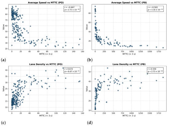
Figure 21.
Comparison of density and the number of HMTTC occurrences. (a) Scatter plot of density vs. HMTTC for the Pangyo–Osan section with fitted regression line. (b) Scatter plot of density vs. HMTTC for the Pangyo–Banpo section. (c) Scatter plot of inverse speed vs. HMTTC for the Pangyo–Osan section. (d) Scatter plot of inverse speed vs. HMTTC for the Pangyo–Banpo section.
4. Discussion
The comparative summary in Table 6 provides a structured overview of representative traffic safety studies based on different sensing modalities and analytical strategies. Synthesizing these findings yields three key insights that clarify the contribution of the proposed framework.
Table 6.
Comparative summary of representative AI and sensor-based traffic safety studies.
First, prior surrogate safety studies have largely relied on single-dimensional indicators such as TTC or PET, which capture only temporal proximity between vehicles [4,14,18]. Although effective for detecting imminent conflicts, these metrics offer limited spatial interpretability and are often constrained to simulation environments or 2D perception domains. In contrast, the present study extends conventional surrogate indicators by introducing HMTTC and SSS, two metrics that jointly consider temporal risk and spatial maneuverability. Leveraging 3D LiDAR geometry enables the proposed system to assess multi-lane interactions and lateral evasive potential, providing a more comprehensive lane-level safety evaluation.
Second, sensor modality plays a critical role in determining the scope and fidelity of risk assessment. Camera- and GPS-based systems [5,17] provide lightweight temporal information but are sensitive to illumination, occlusions, and low spatial resolution. Radar-based systems [43,45] offer robustness in adverse conditions but lack dense spatial detail and exhibit limited angular resolution. By contrast, the vehicle-mounted LiDAR used in this study supplies high-resolution 3D geometry necessary for continuous tracking of surrounding vehicles and for computing HMTTC and SSS. This richer geometric representation bridges the gap between microscopic movement analysis and macroscopic safety assessment, enabling more reliable estimation of interaction-based surrogate safety indicators.
Third, while simulation-based works such as those by Gettman and Head [14] or Ozbay et al. [22] have contributed significantly to surrogate safety methodology, they remain limited by synthetic environments. The present study distinguishes itself by validating its framework using real-world data collected from complex Korean expressways characterized by diverse lighting conditions, dynamic congestion patterns, and frequent merging influences. This empirical validation demonstrates the practical feasibility of interpreting surrogate safety metrics directly from field-measured LiDAR data.
In summary, the proposed AI–LiDAR framework advances surrogate safety research in three major ways: (1) by integrating deep learning–based 3D object detection with quantitative safety modeling, (2) by extending surrogate indicators to incorporate 3D spatial and lane-level risk characteristics, and (3) by demonstrating applicability under real-world urban expressway conditions rather than controlled simulation environments. These contributions collectively address key limitations of prior work and support the development of a scalable, data-driven methodology for urban traffic safety assessment.
Finally, the findings from the experimental evaluation establish a clear empirical foundation for the proposed framework. In particular, the observed relationships among HMTTC, lane-level speed, and density indicate that the metric behaves consistently with established congestion–risk dynamics. This provides strong justification for its use as a congestion-sensitive surrogate safety indicator in practice. Future research may extend this framework by incorporating multi-sensor fusion or modeling more complex driver–vehicle interactions to enable more robust predictive safety assessment.
5. Conclusions
This study highlights the need for advanced traffic monitoring and analysis methods that align with the era of autonomous and connected vehicles. By utilizing vehicle-mounted LiDAR as a dynamic remote sensing platform, the proposed approach enables continuous and high-resolution observation of lane-level traffic conditions on urban and highway corridors.
From a methodological standpoint, we first established an appropriate TTC-based surrogate safety threshold for Korean highway environments. By comparing prior work by Oh et al. [46] with MTTC distributions derived from field data on the Pangyo–Osan and Pangyo–Seocho sections (Figure 11, Figure 12 and Figure 13, Table 3 and Table 4), we verified that a 3 s threshold is both empirically reasonable and sensitive to changes in operational risk. MTTC values below this threshold were defined as HMTTC and adopted as the core surrogate safety indicator in the proposed framework.
Using LiDAR-based measurements, we then demonstrated that lane-specific traffic states cannot be adequately captured by conventional segment-averaged indicators. The results in Figure 14, Figure 15, Figure 16 and Figure 17 show substantial differences in speed and density between lanes, particularly between the bus-only lane and general-purpose lanes, as well as at locations influenced by ramps and junctions. These experiments confirmed that relying solely on overall average speed masks important lane-level variations and can lead to discrepancies with navigation-based traffic information. In contrast, the proposed method provides fine-grained lane-level estimates of speed, density, and TTC, enabling more detailed diagnosis of local bottlenecks and flow transitions.
A safety evaluation was conducted by analyzing the spatial distribution of HMTTC events together with speed and density. The hotspot maps in Figure 18 reveal that HMTTC occurrences tend to concentrate near interchange influence areas on less congested segments, while in persistently congested sections they are more diffusely distributed. When HMTTC counts are jointly examined with density and speed (Figure 19 and Figure 20), a clear association emerges: higher density and lower speed coincide with elevated HMTTC occurrences, especially around ramp influence zones. Pearson correlation analysis (Table 5, Figure 21) further quantified these relationships, indicating statistically significant moderate correlations between HMTTC and both congestion-related density and speed indices. These findings support the interpretation of HMTTC as a congestion-sensitive surrogate safety measure that reflects lane-level operational risk rather than merely counting rare extreme events.
Overall, the proposed HMTTC- and SSS-based framework demonstrates that LiDAR-equipped probe vehicles can be used not only to monitor lane-specific speed and density, but also to identify hazardous locations where evasive safety space is depleted. The color-coded visualization of evasive space and HMTTC hotspots provides an intuitive tool for diagnosing safety-critical areas in real traffic (Figure 10, Figure 11, Figure 12 and Figure 13). Although the present study is limited to data collected from a single probe vehicle and to weather conditions excluding heavy rain and fog, the results confirm the feasibility of LiDAR-based lane-level safety monitoring in complex Korean highway environments.
Future work will extend this framework by deploying multiple sensor-equipped vehicles to form a mobile sensing network and by integrating additional sensing modalities such as 4D Radar to improve robustness under adverse weather conditions. Combining LiDAR-derived point clouds with high-definition (HD) maps and AI-based feature extraction techniques will further enhance real-time hazard detection and support decision-making for intelligent transportation systems. Long-term data accumulation and interdisciplinary collaboration among experts in AI, sensing, and traffic engineering will be essential to establish resilient, data-driven urban traffic management frameworks built upon the proposed methodology.
Author Contributions
Conceptualization, D.K. and W.K.; methodology, D.K. and H.K.; validation, D.K. and H.K.; formal analysis, H.K.; investigation, D.K.; resources, W.K.; data curation, H.K.; writing—original draft preparation, D.K.; writing—review and editing, W.K.; visualization, D.K.; supervision, W.K.; project administration, W.K.; funding acquisition, W.K. All authors have read and agreed to the published version of the manuscript.
Funding
This research was supported by the Culture, Sports and Tourism R&D Program through the Korea Creative Content Agency grant funded by the Ministry of Culture, Sports and Tourism in 2024 (Grant Number: RS-2024-00398310), and by the Ministry of Trade, Industry and Energy (MOTIE) and the Korea Evaluation Institute of Industrial Technology (KEIT) (Grant Number: RS-2024-00487113).
Data Availability Statement
The training and validation datasets used in this study were sourced from the AI Hub Robust Sensor Fusion Object Detection for Autonomous Driving Dataset (https://www.aihub.or.kr/aihubdata/data/view.do?dataSetSn=629, accessed on 27 December 2024). This dataset was utilized for model training, evaluation, and validation. Access to the dataset is governed by AI Hub’s licensing terms and conditions. Any additional processed data derived from this dataset, including re-split data and model outputs, can be made available upon reasonable request to the corresponding author.
Conflicts of Interest
The authors declare no conflicts of interest.
References
- Daganzo, C.F. Fundamentals of Transportation and Traffic Operations; Emerald Group Publishing Limited: Leeds, UK, 1997. [Google Scholar]
- Kim, D.; Kim, H.; Han, S.; Kim, W. Highway Condition Analysis and Traffic Safety Monitoring System Through Analysis of Time-Series Data from LiDAR-based Probe Vehicle. In Proceedings of the 2023 IEEE International Conference on Systems, Man, and Cybernetics (SMC), Honolulu, HI, USA, 1–4 October 2023; pp. 1500–1505. [Google Scholar]
- Shi, C.; Chen, B.Y.; Li, Q. Estimation of travel time distributions in urban road networks using low-frequency floating car data. ISPRS Int. J.-Geo-Inf. 2017, 6, 253. [Google Scholar] [CrossRef]
- Seo, T.; Kusakabe, T.; Asakura, Y. Estimation of flow and density using probe vehicles with spacing measurement equipment. Transp. Res. Part C Emerg. Technol. 2015, 53, 134–150. [Google Scholar] [CrossRef]
- Seo, T.; Kusakabe, T. Probe vehicle-based traffic state estimation method with spacing information and conservation law. Transp. Res. Part C Emerg. Technol. 2015, 59, 391–403. [Google Scholar] [CrossRef]
- Seo, T.; Kusakabe, T.; Asakura, Y. Traffic state estimation with the advanced probe vehicles using data assimilation. In Proceedings of the 2015 IEEE 18th International Conference on Intelligent Transportation Systems, Gran Canaria, Spain, 15–18 September 2015; pp. 824–830. [Google Scholar]
- Gettman, D.; Pu, L.; Sayed, T.; Shelby, S.G.; Siemens Energy and Automation, Business Unit Intelligent Transportation Systems. Surrogate Safety Assessment Model and Validation; Technical Report No. FHWA-HRT-08-051; Turner-Fairbank Highway Research Center: McLean, VA, USA, 2008. [Google Scholar]
- Mahmud, S.S.; Ferreira, L.; Hoque, M.S.; Tavassoli, A. Application of proximal surrogate indicators for safety evaluation: A review of recent developments and research needs. IATSS Res. 2017, 41, 153–163. [Google Scholar] [CrossRef]
- Peng, L.; Lyu, N.; Wu, C. A Road Traffic Crash Risk Assessment Method Using Vehicle Trajectory Data and Surrogate Safety Measures. In Proceedings of the 20th COTA International Conference of Transportation Professionals, Xi’an, China, 14–16 August 2020; pp. 3657–3669. [Google Scholar]
- Amini, R.E.; Yang, K.; Antoniou, C. Development of a conflict risk evaluation model to assess pedestrian safety in interaction with vehicles. Accid. Anal. Prev. 2022, 175, 106773. [Google Scholar] [CrossRef] [PubMed]
- Van der Horst, A.; Hogema, J. Time-to-collision and collision avoidance systems. In Proceedings of the 6th ICTCT Workshop; Austrian Road Safety Board: Vienna, Austria, 1994; pp. 59–63. [Google Scholar]
- Touran, A.; Brackstone, M.A.; McDonald, M. A collision model for safety evaluation of autonomous intelligent cruise control. Accid. Anal. Prev. 1999, 31, 567–578. [Google Scholar] [CrossRef] [PubMed]
- Lee, J.D.; McGehee, D.V.; Brown, T.L.; Reyes, M.L. Collision warning timing, driver distraction, and driver response to imminent rear-end collisions in a high-fidelity driving simulator. Hum. Factors 2002, 44, 314–334. [Google Scholar] [CrossRef]
- Gettman, D.; Head, L. Surrogate safety measures from traffic simulation models. Transp. Res. Rec. 2003, 1840, 104–115. [Google Scholar] [CrossRef]
- Vogel, K. A comparison of headway and time to collision as safety indicators. Accid. Anal. Prev. 2003, 35, 427–433. [Google Scholar] [CrossRef]
- Hourdos, J.N.; Garg, V.; Michalopoulos, P.G.; Davis, G.A. Real-time detection of crash-prone conditions at freeway high-crash locations. Transp. Res. Rec. 2006, 1968, 83–91. [Google Scholar] [CrossRef]
- Guido, G.; Vitale, A.; Astarita, V.; Saccomanno, F.; Giofré, V.P.; Gallelli, V. Estimation of safety performance measures from smartphone sensors. Procedia-Soc. Behav. Sci. 2012, 54, 1095–1103. [Google Scholar] [CrossRef]
- Hayward, J.C. Near Miss Determination Through Use of a Scale of Danger; Pennsylvania Transportation and Traffic Safety Center: Harrisburg, PA, USA, 1972. [Google Scholar]
- Lodinger, N.R.; DeLucia, P.R. Does automated driving affect time-to-collision judgments? Transp. Res. Part F Traffic Psychol. Behav. 2019, 64, 25–37. [Google Scholar] [CrossRef]
- Jiménez, F.; Naranjo, J.E.; García, F. An improved method to calculate the time-to-collision of two vehicles. Int. J. Intell. Transp. Syst. Res. 2013, 11, 34–42. [Google Scholar] [CrossRef]
- Montgomery, J.; Kusano, K.D.; Gabler, H.C. Age and gender differences in time to collision at braking from the 100-car naturalistic driving study. Traffic Inj. Prev. 2014, 15, S15–S20. [Google Scholar] [CrossRef]
- Ozbay, K.; Yang, H.; Bartin, B.; Mudigonda, S. Derivation and validation of new simulation-based surrogate safety measure. Transp. Res. Rec. 2008, 2083, 105–113. [Google Scholar] [CrossRef]
- Minderhoud, M.M.; Bovy, P.H. Extended time-to-collision measures for road traffic safety assessment. Accid. Anal. Prev. 2001, 33, 89–97. [Google Scholar] [CrossRef]
- Behbahani, H.; Nadimi, N.; Naseralavi, S. New time-based surrogate safety measure to assess crash risk in car-following scenarios. Transp. Lett. 2015, 7, 229–238. [Google Scholar] [CrossRef]
- Kiefer, R.J.; LeBlanc, D.J.; Flannagan, C.A. Developing an inverse time-to-collision crash alert timing approach based on drivers’ last-second braking and steering judgments. Accid. Anal. Prev. 2005, 37, 295–303. [Google Scholar] [CrossRef] [PubMed]
- Xie, K.; Yang, D.; Ozbay, K.; Yang, H. Use of real-world connected vehicle data in identifying high-risk locations based on a new surrogate safety measure. Accid. Anal. Prev. 2019, 125, 311–319. [Google Scholar] [CrossRef]
- Kuang, Y.; Qu, X. Applicability Analysis of Aggregated Crash Index (ACI) in Freeways. In Proceedings of the Engineering, Project, and Production Management (EPPM) Conference, Gold Coast, QLD, Australia, 2–4 September 2015. [Google Scholar]
- Tak, S.; Kim, S.; Yeo, H. Development of a deceleration-based surrogate safety measure for rear-end collision risk. IEEE Trans. Intell. Transp. Syst. 2015, 16, 2435–2445. [Google Scholar] [CrossRef]
- Laureshyn, A.; Svensson, Å.; Hydén, C. Evaluation of traffic safety, based on micro-level behavioural data: Theoretical framework and first implementation. Accid. Anal. Prev. 2010, 42, 1637–1646. [Google Scholar] [CrossRef]
- Fanti, M.P.; Iacobellis, G.; Ukovich, W. A risk assessment framework for Hazmat transportation in highways by colored Petri nets. IEEE Trans. Syst. Man Cybern. Syst. 2014, 45, 485–495. [Google Scholar] [CrossRef]
- Zhang, H.; Luo, G.; Li, Y.; Wang, F.Y. Parallel vision for intelligent transportation systems in metaverse: Challenges, solutions, and potential applications. IEEE Trans. Syst. Man Cybern. Syst. 2022, 53, 3400–3413. [Google Scholar] [CrossRef]
- Gao, H.; Zhu, J.; Zhang, T.; Xie, G.; Kan, Z.; Hao, Z.; Liu, K. Situational assessment for intelligent vehicles based on stochastic model and Gaussian distributions in typical traffic scenarios. IEEE Trans. Syst. Man Cybern. Syst. 2020, 52, 1426–1436. [Google Scholar]
- Das, S.; Mustavee, S.; Agarwal, S.; Hasan, S. Koopman-theoretic modeling of quasiperiodically driven systems: Example of signalized traffic corridor. IEEE Trans. Syst. Man Cybern. Syst. 2023, 53, 4466–4476. [Google Scholar] [CrossRef]
- Liao, X.; Zhao, X.; Wang, Z.; Han, K.; Tiwari, P.; Barth, M.J.; Wu, G. Game theory-based ramp merging for mixed traffic with unity-sumo co-simulation. IEEE Trans. Syst. Man Cybern. Syst. 2021, 52, 5746–5757. [Google Scholar] [CrossRef]
- Wang, X.; Zheng, X.; Chen, W.; Wang, F.Y. Visual human–computer interactions for intelligent vehicles and intelligent transportation systems: The state of the art and future directions. IEEE Trans. Syst. Man Cybern. Syst. 2020, 51, 253–265. [Google Scholar] [CrossRef]
- Tan, F.; Zhai, M.; Zhai, C. Foreign object detection in urban rail transit based on deep differentiation segmentation neural network. Heliyon 2024, 10, e37072. [Google Scholar] [CrossRef]
- Tan, F.; Liu, K.; Li, L.; Yang, W. An Intelligent Detection System for Full Crew of Elevator Car. In Proceedings of the 2018 11th International Conference on Intelligent Computation Technology and Automation (ICICTA), Changsha, China, 22–23 September 2018; pp. 183–185. [Google Scholar]
- Deng, J.; Shi, S.; Li, P.; Zhou, W.; Zhang, Y.; Li, H. Voxel R-CNN: Towards high performance voxel-based 3D object detection. In Proceedings of the AAAI Conference on Artificial Intelligence, Online, 2–9 February 2021; Volume 35, pp. 1201–1209. [Google Scholar]
- Yin, T.; Zhou, X.; Krahenbuhl, P. CenterPoint: Center-based 3D Object Detection and Tracking. In Proceedings of the IEEE/CVF Conference on Computer Vision and Pattern Recognition (CVPR), Nashville, TN, USA, 19–25 June 2021; pp. 11784–11793. [Google Scholar]
- Bai, X.; Hu, Z.; Zhu, X.; Huang, Q.; Chen, Y.; Fu, H.; Tai, C.L. TransFusion: Robust LiDAR-Camera Fusion for 3D Object Detection with Transformers. In Proceedings of the IEEE/CVF Conference on Computer Vision and Pattern Recognition (CVPR), New Orleans, LA, USA, 18–24 June 2022; pp. 1080–1089. [Google Scholar]
- Choi, S.; Kim, D.; Park, S.; Paik, J. Point cloud-based lane detection for optimal local path planning. In Proceedings of the 2022 International Conference on Electronics, Information, and Communication (ICEIC), Jeju, Republic of Korea, 6–9 February 2022; pp. 1–4. [Google Scholar]
- Wakasugi, T. A study on warning timing for lane change decision aid systems based on drivers lane change maneuver. In Proceedings of the 19th International Technical Conference on the Enhanced Safety of Vehicles, Washington, DC, USA, 6–9 June 2005; p. 05-0290. [Google Scholar]
- Corral-Soto, E.R.; Grandhi, A.; He, Y.Y.; Rochan, M.; Liu, B. Improving lidar 3d object detection via range-based point cloud density optimization. arXiv 2023, arXiv:2306.05663. [Google Scholar]
- Peri, N.; Li, M.; Wilson, B.; Wang, Y.X.; Hays, J.; Ramanan, D. An empirical analysis of range for 3d object detection. In Proceedings of the IEEE/CVF International Conference on Computer Vision, Paris, France, 2–3 October 2023; pp. 4074–4083. [Google Scholar]
- Khoche, A.; Sánchez, L.P.; Batool, N.; Mansouri, S.S.; Jensfelt, P. Towards long-range 3D object detection for autonomous vehicles. In Proceedings of the 2024 IEEE Intelligent Vehicles Symposium (IV), Jeju Island, Republic of Korea, 2–5 June 2024; pp. 2206–2212. [Google Scholar]
- Oh, C.; Jo, J.-I.; Kim, J.-H.; Oh, J.-T. Methodology for Evaluating Real-Time Rear-End Collision Risks Based on Vehicle Trajectory Data Extracted from Video Image Tracking. J. Korean Soc. Transp. 2007, 25, 173–182. [Google Scholar]
- Pearson, K., VII. Note on regression and inheritance in the case of two parents. Proc. R. Soc. Lond. 1895, 58, 240–242. [Google Scholar]
- Moore, D.S.; McCabe, G.P.; Craig, B.A. Introduction to the Practice of Statistics; WH Freeman: New York, NY, USA, 2009; Volume 4. [Google Scholar]
Disclaimer/Publisher’s Note: The statements, opinions and data contained in all publications are solely those of the individual author(s) and contributor(s) and not of MDPI and/or the editor(s). MDPI and/or the editor(s) disclaim responsibility for any injury to people or property resulting from any ideas, methods, instructions or products referred to in the content. |
© 2025 by the authors. Licensee MDPI, Basel, Switzerland. This article is an open access article distributed under the terms and conditions of the Creative Commons Attribution (CC BY) license (https://creativecommons.org/licenses/by/4.0/).