High-Resolution Retrieval of Radial Ocean Current Velocity from SAR Strip-Map Imagery

Highlights

What are the main findings?

• A novel high-resolution radial ocean surface current (OSC) velocity estimation method is proposed, utilizing Maximum A Posteriori (MAP) estimation based on signal modeling of the local Doppler power spectrum.
• Compared with existing algorithms, the proposed method substantially improves retrieval accuracy while effectively resolving the azimuth doppler ambiguity problem.

What are the implications of the main findings?

• Obtaining more precise and reliable radial OSC data from SAR is crucial for ocean current research.
• The proposed method is beneficial for high-resolution operational ocean monitoring utilizing SAR image data.

Abstract

The retrieval of radial ocean surface current from Synthetic Aperture Radar (SAR) data is important for ocean current research and effective ocean remote sensing. Existing algorithms, primarily based on the Average Cross-Correlation Coefficient (ACCC) method, suffer from drawbacks, including low Doppler frequency-shift estimation accuracy and susceptibility to azimuth ambiguity, hindering accurate measurements. To address these limitations, this paper proposes a method for high-resolution radial current velocity estimation. This approach employs Maximum A Posteriori (MAP) estimation based on signal modeling of the local Doppler power spectrum. This method achieves better Doppler frequency shift estimation accuracy than ACCC and effectively mitigates the azimuth ambiguity, substantially enhancing the precision of radial ocean surface velocity estimation. The algorithm was validated using raw Sentinel-1 Strip-map mode real data and HYCOM data acquired over the Seychelles Islands on 23 April 2023, and the central Indian Ocean (south of the equator) on 20 May 2023. Compared with the Sentinel-1 Level 2 ocean Surface Radial Velocity (RVL) product, the method demonstrates the improvements in both spatial resolution and retrieval accuracy. Specifically, the quantitative comparison with HYCOM data showed a reduction in Root Mean Square Error (RMSE) of up to 34.3% and an improvement in Mean Absolute Error (MAE) of up to 32.1%. Moreover, its ability to suppress the azimuth Doppler ambiguity is demonstrated in the real-data experiment.

1. Introduction

Ocean current motion is a fundamental marine physical phenomenon that influences ocean transport and impacts global climate change [1]. The rapid development of remote sensing technology has enabled large-area, high-precision, and comprehensive observation and study of ocean currents [1]. Ocean current observation and research provide essential support for uncovering the mechanisms of interaction among the ocean, land, and atmosphere, and serve as a necessary prerequisite for developing marine disaster early warning systems. Sensors commonly used for ocean current remote sensing observation typically include altimeters [2,3], High-Frequency (HF) radar [4], and Synthetic Aperture Radar (SAR) [5]. The retrieval of geostrophic currents from altimeter data is based on the Coriolis force balance equation, with these currents accounting for only a part of the total ocean current. However, the spatial resolution of these methods is relatively low (approximately 25 km [6]), leading to inaccurate measurements of current motion formed by small-scale ocean phenomena [7,8]. Furthermore, these products are not suitable for retrieving ocean surface currents in coastal areas [9]. HF radar is a widely used method for measuring ocean surface currents, but these sensors are primarily deployed near the coast, thereby limiting data acquisition from remote ocean regions [10].

The SAR, with its all-weather, all-time, high-resolution, and wide-swath characteristics, offers an un-substitutable advantage in ocean current observation. After nearly 60 years of development, SAR has been successfully applied to observe many oceanic elements, including ocean currents [11]. Currently, there are two main techniques for observing ocean currents using SAR. The first is the Along-Track Interferometric (ATI) SAR measurement method [12], whose basic principle uses the phase difference between two interferometric SAR images and the Doppler frequency shift to retrieve the radial ocean current velocity. Although ATI technology can retrieve radial ocean current velocity with high precision and high resolution, most existing spaceborne ATI experiments utilize a single-satellite, dual-antenna, short-baseline mode, resulting in a scarcity of data. Examples include TanDEM-X, SRTM-SAR, RadarSat-2, TerraSAR-X, and Gaofen-3. The effective baseline length for TanDEM-X ranges from 25 m to 40 m [13]; SRTM-SAR utilized an additional 7 m along-track antenna separation on the space shuttle [14]; TerraSAR-X in DRA mode has an effective baseline of only 1.15 m [13]; and Gaofen-3’s effective ATI baseline length is 3.75 m [15]. If a short baseline aims to achieve the same ocean current retrieval accuracy as a long baseline, the radial current velocity resolution must be reduced [13]. In ATI technology, selecting a reasonable baseline length to balance retrieval resolution and accuracy remains a challenge. Currently, an operational framework for SAR satellite-based ATI-SAR current observation has not yet been established, hindering widespread research on ocean current retrieval from SAR images [16,17]. The second retrieval method is based on Doppler Centroid Anomaly (DCA) estimation. The DCA method for measuring ocean currents was first proposed by [18], and subsequently theoretically and experimentally verified using Radarsat-1 by Hutt et al. [19]. Chapron [6] first analyzed the theory underlying the modeling and analysis of Doppler information. Their study assessed the feasibility of retrieving the radial ocean current velocity, examined the relationship between the Doppler frequency shift and the backscattering coefficient, proposed a simplified Doppler centroid model, and analyzed possible sources of bias in Doppler frequency-shift estimation. The DCA method has been widely used for ocean current measurements across numerous spaceborne platforms. Among these platforms, Sentinel-1 SAR data is widely used and has been applied to produce the Sea Surface Radial Velocity (RVL) product [20]. For Strip-map (SM), Interferometric Wide Swath (IW), and Extra Wide Swath (EW) modes, the RVL product’s spatial resolution is 1.5 × 1.7 km, 2 × 2 km, and 4 × 4 km, respectively, while in Wave (WV) mode, the resolution is 20 km. Envisat ASAR also provided a Doppler centroid grid data product, with a resolution of 3.5 km to 9 km in the range direction and 8 km in the azimuth direction. Furthermore, Romeiser et al. compared DCA-measured results with TerraSAR-X DRA-mode results at short baselines and found similar accuracy at the exact resolution [13]. Although the DCA method is a good alternative to ATI technology in DRA mode [13], its accuracy has not yet reached that of the ATI method under long-baseline conditions. Nevertheless, the DCA method utilizes SAR data to achieve a spatial resolution superior to that of other sensors, making it suitable for high-resolution current observation and ship velocity measurement [21]. Therefore, research utilizing the DCA method for current retrieval is significant.

The DCA method is a Doppler frequency shift estimation technique for SAR signals, which is not a new problem. Doppler frequency shift estimation methods are generally classified into two categories: methods based on the Doppler Power Spectrum (DPS) and methods based on the phase of the autocorrelation function. Bamler has proposed a Doppler centroid estimation method based on the DPS, whose accuracy can approach the Cramér–Rao Bound [22]. However, this method is highly dependent on a priori information, requiring the prior acquisition of parameters such as antenna patterns, noise characteristics, and azimuth ambiguity. While this information is relatively easy to obtain in the overall estimation of radar signals, it is difficult to apply to per-grid Doppler shift estimation, thereby limiting its widespread use in ocean surface radial velocity retrieval. In contrast, the ACCC method is currently the widely used method for radial ocean current velocity estimation [23,24,25]. Notably, although Sentinel-1’s Doppler product is also constructed using a Doppler spectrum model [26] that estimates the Doppler frequency shift by analyzing the relationship between the first-order inverse Fourier coefficient and the autocorrelation function, the results indicate that the influence of azimuth ambiguity persists within the study area. In SAR systems, azimuth ambiguity is an inherent property of SAR signal processing, arising from moving targets or strong scatterers in the azimuth direction and leading to aliasing of the radar signal’s DPS. This aliasing results in azimuth ambiguity—namely, energy wraparound in the SAR azimuth direction. Crucially, these ambiguous signals severely affect the accuracy of Doppler frequency shift estimation. Previous researchers have conducted extensive research on azimuth ambiguity. Villano et al. estimated the Azimuth Ambiguity-to-Signal Ratio (AASR) of the left and right ambiguous regions from the Doppler spectrum by constructing a Wiener filtering function for the corresponding area [27]. Sun et al. estimated the AASR of the left and right ambiguous regions from SAR images using the aforementioned method and studied the impact of these regions on Doppler frequency shift estimation through modeling [28]. However, these efforts have not effectively mitigated the effect of azimuth ambiguity on Doppler frequency shift estimation.

To overcome the limitations of traditional algorithms in Doppler frequency estimation accuracy and azimuth ambiguity, this paper presents a new method for retrieving radial ocean current velocity. By modeling the local DPS of SAR SLC data within a Maximum a Posteriori (MAP) estimation framework, the proposed approach achieves precise Doppler estimation and effectively eliminates azimuth ambiguities. In this paper, the method offers a “High-Resolution” capability—defined as a medium-resolution improvement from the standard 1 km Sentinel-1 RVL product to approximately a 500 m grid. This enhancement is important for detecting sub-mesoscale features, such as small eddies, which are often smoothed out in conventional kilometer-scale products. For theoretical validation, simulation results demonstrate that, compared to the ACCC method, the proposed method achieves higher precision, with its accuracy approaching the Cramér–Rao Lower Bound (CRLB). For real-data validation, we used raw Sentinel-1 SM-mode data, performing decoding [29] and imaging [30] operations to obtain azimuth-unweighted SAR SLC images, and subsequently retrieved the radial ocean current from these images. To evaluate the proposed method’s improvement in spatial resolution and fine-scale texture of the retrieved radial ocean surface current. The compelling evidence for the preservation of fine-scale detail is the High-Frequency Spectral Energy Ratio. The value obtained by the proposed method (0.101) is more than double that of the Sentinel-1 RVL product (0.048), confirming a substantial retention of high-wavenumber (fine-scale) energy. In terms of spatial resolution, the proposed method achieves a substantial reduction, yielding approximately 54.5% and 45.9% improvements in the Azimuth and Range directions, respectively, compared to the Sentinel-1 RVL product. These metrics consistently confirm that the proposed algorithm not only achieves substantially higher spatial resolution but also enhances the fine-scale variability and structural quality of the retrieval results relative to the Sentinel-1 RVL product. In the comparative validation with the HYCOM model, the proposed method demonstrated clear performance improvements. Specifically, the Mean Absolute Error (MAE) and Root Mean Square Error (RMSE) were reduced by 32.1% and 34.3%, respectively, while the correlation coefficient (R) increased from 0.590 to 0.705. These consistent, quantifiable improvements strongly confirm that, relative to the Sentinel-1 RVL product, the proposed method provides a more accurate and reliable estimate of the radial ocean surface velocity. Furthermore, real-data experiments explicitly verified its capability to eliminate azimuth Doppler ambiguity. Therefore, the proposed method offers a radial ocean current velocity retrieval solution for ocean remote sensing monitoring that is characterized by high resolution, high accuracy.

2. Doppler Frequency Shift Estimation Method

2.1. The Model and Method for Doppler Shift Estimation

Theoretically, SLC SAR data follows a complex Gaussian distribution with independent components. The SLC SAR image data at sampling time ∆t to arrange the complex vector [22]:

$$u=u_s+u_n=[u(1),\cdot \cdot \cdot ,u(k),\cdot \cdot \cdot ,u(N)],$$

(1)

where $u_s$ is the SAR image signal, and $u_n$ represents the SAR image noise. N denotes the total number of samples, and k represents the sample index (k = 1, …, N). $u$ represents data in the azimuth direction. After the discrete Fourier transform, $U$ can be written as:

$$U=U_s+U_n=[U(1),\cdot \cdot \cdot ,U(k),\cdot \cdot \cdot ,U(N)],$$

(2)

$U_s$ and noise $U_n$ are complex Gaussian, zero-mean, and orthogonal processes. Thus, the spectrum samples $U(k)$ are uncorrelated. Thus, the DPS of SLC SAR images can be considered as:

$$S=[S(f_1),\cdot \cdot \cdot ,S(f_k),\cdot \cdot \cdot ,S(f_N)]=[{\left|U(1)\right|}^2,\cdot \cdot \cdot ,{\left|U(k)\right|}^2,\cdot \cdot \cdot ,{\left|U(N)\right|}^2],$$

(3)

$f_k$ is the Doppler frequency range from −PRF/2 to PRF/2, and PRF is the pulse repetition frequency of the spaceborne system. Since U is a complex Gaussian process, S follows an exponential distribution. For SAR imagery data, the average DPS, after averaging m independent samples in the range direction, follows a Gamma distribution [31]. Thus, the averaged DPS probability density function (PDF) can be expressed as follows:

$$p[S(f_k)]=1/\Gamma (m){\left\{m/E\left[S(f_k)\right]\right\}}^m{[S(f_k)]}^{(m-1)}\exp [-mS(f_k)/E\left[S(f_k)\right],$$

(4)

$\Gamma (m)$ is the Gamma function, respectively. The average DPS $E(S(f_k))$ within the above statistical model can be expressed through the modeling [22]:

$$E\left[S(f_k)\right]={\displaystyle \sum _{n=-\infty }^{n=\propto }\overline{\sigma }}(x_0+n{D}_x,y_0+n{D}_y)P_a(f_k-f_d^n+nPRF)+N_0,$$

(5)

$$P_a(f)=\sin c{(f/b)}^4,$$

(6)

here, $\left(x_0,y_0\right)$ refers to the central coordinate of the local statistical data grid. The coordinates $x_0$ and $y_0$ correspond to the range direction and azimuth direction, respectively. Let n be an integer. The n = 0 term refers to the signal from the main lobe, while all non-zero integer values n correspond to the data grids of the azimuth ambiguity signals. The $f_d^n$ is the Doppler shifts, and $\overline{\sigma }\left(x_0+n{D}_x,y_0+n{D}_y\right)$ is the average Radar Cross-Section (RCS) of the data grid along with the azimuth direction. $P_a\left(f\right)$ is the two-way antenna gain pattern function. b is the antenna pattern shape factor. $N_0$ is the noise component within the DPS, which essentially corresponds to white Gaussian noise. The background noise level encountered in SAR image is fundamentally dictated by the intrinsic properties of the radar system. $D_{azi}$ and $D_{rg}$ are the displacements between the position of the azimuthal ambiguity and the corresponding real target in the azimuth and range directions, respectively. These displacements can be written as follows [32]:

$$D_{azi}={\displaystyle \frac{R\lambda F_r}{2V}},D_{rg}=-{\displaystyle \frac{f_0{\lambda }^{2}R{F}_r}{4V^2}},$$

(7)

where R is the slant range of the target, $\lambda$ is the radar wavelength, $F_r$ is the PRF, $V$ is the satellite’s velocity, and $f_0$ is the Doppler centroid of the target. When using Formula (5), analysis is generally restricted to three of its terms, and the justification for this simplification will be presented in Section 2.3. It can thus be approximately written as:

$$\begin{array}{c}E\left[S\left(f_k\right)\right]={{\displaystyle \sum }}_{n=-1}^{n=1}\overline{\sigma }\left(x_0+n{D}_x,y_0+n{D}_y\right)P_a\left(f_k-f_d^n+nPRF\right)+N_0\\ \approx {\sigma }_0{P}_a\left(f_k-f_d\right)+{\sigma }_R{P}_a\left(f_k-f_{dR}+F_r\right)+{\sigma }_L{P}_a\left(f_k-f_{dL}-F_r\right)+N_0\end{array},$$

(8)

where ${\sigma }_0{P}_a(f_i-f_d)$ denotes the DPS of the main lobe signal, ${\sigma }_0$ is equal to $\overline{\sigma }(x_0,y_0)$, $f_d$ is equal to $f_d^0$ which is the Doppler frequency shift in main lobe signal. ${\sigma }_R{P}_a(f_k-f_{dR}+F_r)$ denotes the DPS of the first right azimuth ambiguity signal, ${\sigma }_R$ is equal to $\overline{\sigma }(x_0+D_x,y_0+D_y)$ which denotes the average scattering value of the first right azimuth ambiguity signal, $f_{dR}$ is equal to $f_d^{+1}$ which is the Doppler frequency shift resulting from the first right ambiguity signal. ${\sigma }_L{P}_a(f_k-f_{dL}-F_r)$ denotes the DPS of the first left azimuth ambiguity signal, ${\sigma }_L$ is equal to $\overline{\sigma }(x_0-D_x,y_0-D_y)$ which denotes the average RCS of the first left azimuth ambiguity data grid, $f_{dL}$ is equal to $f_d^{-1}$, which is the Doppler frequency shift resulting from the first left ambiguity. To illustrate the shape differences in the DPS due to system noise, azimuthal ambiguity, and backscattering signal more clearly, a schematic is shown in Figure 1. When the observed signal is not contaminated by azimuth ambiguities due to strong scattering points or moving targets, the amplitude of the left and right ambiguity is close to identical. As shown in the schematic in Figure 1 of the DPS, the SAR simulation image signal is mainly composed of the four parts listed above.

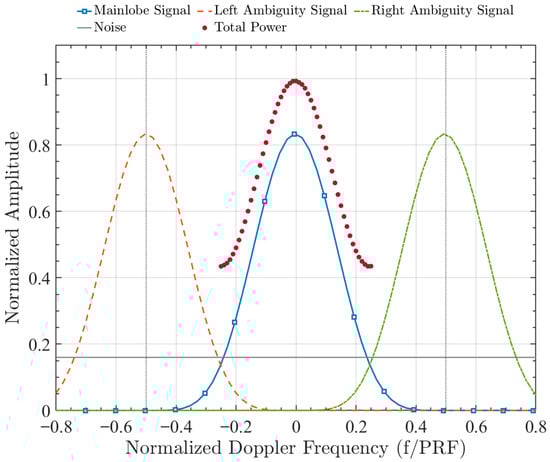
Figure 1. Schematic of the Doppler Power Spectrum (DPS) components. The solid blue line with square markers represents the main lobe signal. The left- and right-azimuth ambiguities are indicated by dashed orange and green lines, respectively. The noise power floor remains flat across all frequencies, as shown by the solid gray line. Finally, the total power is depicted by a dotted red line with circular markers, concentrated near the zero Doppler frequency.

In order to utilize MAP estimation, Equations (4) and (8) can be generalized to the ensemble form of the DPS. Considering that the $f_d$ and ${\sigma }_0$ distributions are independent of each other, through the Bayesian formula expansion, it can be expressed as follows:

$$p(f_d,{\sigma }_0|S)=p(S|f_d,{\sigma }_0)p(f_d)p({\sigma }_0)/p(S),$$

(9)

where $p(S)$ can be a constant, thus:

$$p(f_d,{\sigma }_0|S)\propto p(S|f_d,{\sigma }_0)p(f_d)p({\sigma }_0),$$

(10)

therefore, the problem becomes:

$$\left\{\begin{array}{l}\underset{f_d,{\sigma }_0}{\arg \max } p(f_d,{\sigma }_0|S)=\underset{f_d,{\sigma }_0}{\arg \max } p(S|f_d,{\sigma }_0)p(f_d)p({\sigma }_0)\\ s.t.\begin{array}{c}\end{array}{\sigma }_0\ge 0\end{array}\right.,$$

(11)

where ${\sigma }_0,f_d$ can be regarded as the estimation parameters, namely the average RCS and Doppler frequency shift in the main lobe signal, respectively. $p(f_d)$ is the prior probability density of $f_d$, which is assumed to have a Gaussian distribution with a narrow distribution range, which is expressed as:

$$p(f_d)={\displaystyle \frac{1}{\sqrt{2\pi }{\sigma }_v}}\exp \left[-{\displaystyle \frac{{f_d}^2}{2{{\sigma }_v}^2}}\right],$$

(12)

where ${\sigma }_v$ is the variance of the Doppler shifts, in this study, for the C-band SAR system, in the case of medium sea conditions, considering that the absolute value of the ocean surface radial velocity does not exceed 2 m/s, ${\sigma }_v$ is set to 72 Hz for our model, which can be applied to a general ocean state. $p(S|f_d,{\sigma }_0)$ is defined as the DPS prior probability density, and the statistics of the DPS points are independent of each other.

To accurately estimate the Doppler frequency shift, we also need to estimate the ${\sigma }_0$ of the main-lobe signal. The RCS statistical characterization can be described as a Gamma distribution [33]. Therefore, the PDF of ${\sigma }_0$ can be expressed as:

$$P({\sigma }_0)={\left({\displaystyle \frac{m}{⟨{\sigma }_0⟩}}\right)}^m{\displaystyle \frac{{{\sigma }_0}^{m-1}}{\Gamma (m)}}\exp \left[-{\displaystyle \frac{m{\sigma }_0}{⟨{\sigma }_0⟩}}\right],\begin{array}{cc}& {\sigma }_0\ge 0\end{array},$$

(13)

where m is the number of statistically independent looks, $⟨•⟩$ is the mean operation. It should be noted that the previous model actually contains other variables (${\sigma }_L$, ${\sigma }_R$, $f_{dL}$ and $f_{dR}$). For the MAP estimation, we process these variables by taking the logarithm of the likelihood function of Formula (11). By combining Equations (8), (12) and (13), we can obtain:

$$\begin{array}{l}G({\sigma }_0,{\sigma }_L,{\sigma }_R,f_d,f_{dL},f_{dR})\\ =\{{\displaystyle \sum _{k=1}^N\ln [(m-1)!]-m\ln (m/E[S(f_k)])}-\left(m-1\right)\ln \left[S\left(f_k\right)\right]+(mS\left(f_k\right)/E[S(f_k)])\}\\ +f_d/(2{{\sigma }_v}^2)+\ln \sqrt{2\pi }{\sigma }_v-m\ln (m/⟨{\sigma }_0⟩)-(m-1)\ln {\sigma }_0+\ln (\Gamma (m))+m{\sigma }_0/⟨{\sigma }_0⟩\end{array}$$

(14)

To efficiently solve Equation (14), an alternating minimization strategy is employed, with all variables except the target held fixed. Crucially, parameter identifiability is ensured by specific constraints: the ambiguous Doppler shifts ($f_{dL}$, $f_{dR}$) are not independent variables but are strictly coupled to the main-lobe shift $f_d$ via the geometric relations in Equation (7), while the ambiguity intensities (${\sigma }_L$, ${\sigma }_R$) required to estimate ${\sigma }_0$ are constrained by values from neighboring grids. These constraints effectively ensure a unique solution, reducing the problem to the following sub-problems:

$$\left\{\begin{array}{l}\widehat{{\sigma }_0}=\arg {\min }_{{\sigma }_0}G({\sigma }_0,{\sigma }_L,{\sigma }_R,f_d,f_{dL},f_{dR})\\ s.t.\begin{array}{c}\end{array}{\sigma }_0\ge 0\end{array}\right.,$$

(15)

$$\left\{\begin{array}{l}\widehat{f_d}=\arg {\min }_{f_d}G({\sigma }_0,{\sigma }_L,{\sigma }_R,f_d,f_{dL},f_{dR})\\ s.t.\begin{array}{c}\end{array}{\sigma }_0\ge 0\end{array}\right.,$$

(16)

For the above problems, due to the large number of parameters in this model, and solving the variables ${\sigma }_0$ and $f_d$ of each local data grid needs to use ${\sigma }_{L,R}$ and $f_{L,R}$ parameters will become difficult. To simplify the solution, the Quasi-Alternating Direction Method of Multipliers (quasi-ADMM) is used to optimize the iteration. Unlike the ADMM algorithm, this method provides an approximate solution and can also meet the requirements of parameter estimation.

The Q-ADMM algorithm steps are as follows:

Update the ${\sigma }_0$:

$${\sigma }_0^{(i)}=\arg {\min }_{{\sigma }_0}G({\sigma }_0,{\sigma }_L^{(i-1)},{\sigma }_R^{(i-1)},f_d^{(i-1)},f_{dL}^{(i-1)},f_{dR}^{(i-1)}),$$

(17)

Update the $f_d$:

$$f_d^{(i)}=\arg {\min }_{f_d}G({\sigma }_0^{(i)},{\sigma }_L^{(i)},{\sigma }_R^{(i)},f_d,f_{dL}^{(i-1)},f_{dR}^{(i-1)}),$$

(18)

where i is the iteration count. Each minimization subproblem (Equations (17) and (18)) involves solving a system of two simultaneous equations, which can be performed using Newton’s method. The detailed procedure is described in II-B. For the SAR SLC image data, the Doppler frequency shift $f_d$ estimated through this process generally includes the following parts [24,34]:

$$f_{dc}=f_{\mathrm{e}lec}+f_{att}+\Delta f_{dc}+f_c+f_b+f_l,$$

(19)

where $f_c$ is caused by ocean currents, $f_b$ is caused by the Bragg-wave phase velocity, and $f_l$ is caused by the large-scale wave orbital velocity. The $f_{elec}$ is the antenna electronic mis-pointing term, $f_{att}$ is the error term due to satellite attitude roll, pitch, and yaw deviations, and $\Delta f_{dc}$ is the residual error resulting from the imperfect prediction of non-geophysical terms or other unknown biases. The Sentinel-1 residual variation after recalibration is approximately 3.8 Hz, and the attitude has already been corrected when imaging raw satellite SAR data [24]. In this study, the previous three parts were corrected using Doppler centroid compensation, based on the parameter and auxiliary data files from the XML files. In other words, they can be written as follows [34]:

$$f_d=f_c+f_b+f_l,$$

(20)

where $f_d$ is a geophysical signal related to the ocean RVL by $V_{RVL}=\lambda f_d/2$ (Assuming the satellite radar operates at zero-squint), and $\lambda$ is the radar wavelength. Therefore, the accurate radial Doppler frequency shift in the ocean current is $f_c$. In order to obtain an accurate $f_c$, it is necessary to use the ocean physical model like CDOP [35] to take into account the wind direction and wind speed to obtain the Doppler error caused by the wind. Generally speaking, the Doppler error caused by Bragg scattering is mainly generated by the wind on the sea surface. For the large-scale wave, which is the gravity wave you consider, it is also possible to remove the error Doppler shift through the physical model. Consequently, the $f_d$ estimated by the method proposed in this paper incorporates the above three terms.

2.2. Flowchart and Summary of the Proposed Algorithm

The algorithm used in this method is illustrated in Figure 2. The method of estimating the radial Doppler shift is as follows:

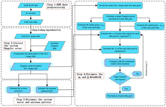
Figure 2. Proposed Workflow for Doppler Frequency Shift Estimation.

2.2.1. RAW Data Preprocessing

Owing to the complex weighting procedures applied to Sentinel-1 SLC product data, the estimation method proposed in this paper is no longer viable. Consequently, we opt to generate SAR SLC images independently—without azimuth weighting—from Sentinel-1 SAR Level 0 (RAW) data. This allows us to employ the proposed estimation method to accurately determine the Doppler frequency shift. Our research employs the MATLAB (R2022b) unpacking routine developed by Ahmed [29].

2.2.2. Correct the System Doppler Error

Following SAR data pre-processing, with the acquired echo data and corresponding radar parameters, the Chirp Scaling Algorithm (CSA) [30] is employed to perform the imaging, which is renowned for its superior phase preservation. According to Equation (19), three types of errors in the Doppler frequency shift are caused by system errors: antenna mis-pointing, satellite attitude roll, pitch, and yaw deviations, and residual errors. These errors need to be removed. SAR SLC data are multiplied by the linear phase term in the time domain to complete the systematic error correction. The linear phase term is determined using auxiliary data file parameters.

2.2.3. Estimate the System Noise and Antenna Pattern

The antenna pattern parameters in Equation (8) are estimated from the SAR SLC image data, specifically using the method detailed in [36]. White noise is present in the SAR signal, which manifests as background noise in the SAR SLC images. We consider the frequency band of the sampling rate that extends beyond the system bandwidth as noise, and use the signal strength in this band as the noise density in the range-frequency domain to estimate the total noise. The processing can be described by the following formula:

$$N_0=S_a\times S_r\times \left(B_r-B_p\right)/S_n/B_p/B_a,$$

(21)

where S_n is the out-of-band noise energy, B_r is the radar system bandwidth, B_p is the range processing bandwidth, S_r is the total energy of the average range power spectrum, Sa is the total energy of the average azimuth DPS, and B_a is the spectrum bandwidth.

2.2.4. Iteratively Estimate ${\sigma }_0$ and $f_d$

In Step 3, the Doppler-centroid-shifted SLC image from Step 1 is divided into many data grids. From the first step of preprocessing, the SAR SLC image has N points in the azimuth direction and M points in the range direction. It is divided into m × n data grids along both the range and azimuth directions, following the principle illustrated in Figure 3.

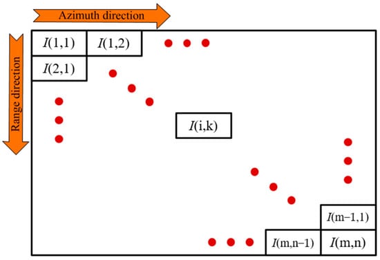
Figure 3. Schematic Diagram of SAR Image dividing.

For each data grid, the local average DPS is estimated first. To solve the optimization problem defined in Equations (15) and (16), we adopt an alternating minimization strategy, referred to here as Quasi-ADMM. Unlike the standard ADMM algorithm which involves dual variable updates and requires tuning penalty parameters, our approach iteratively minimizes the negative log-likelihood function $G(\cdot )$ with respect to one block of variables while holding the others fixed. This formulation eliminates the need for explicit penalty parameters, thereby simplifying the implementation.

To ensure global convergence and reduce computational cost, proper initialization is performed before the iteration. The initial value ${\sigma }_{0\_ini}$ is estimated using the statistical estimation method for low-scattering areas [32], which calculates the mean intensity of the lower percentile of the histogram in the local window. The initial Doppler shift $f_{d\_ini}$ is estimated by the Energy Balancing method [25].

The iterative update process proceeds as follows:

In the update of ${\sigma }_0$ at the i-th step (Equation (17)), $f_d$, ${\sigma }_L$, ${\sigma }_R$, $f_{dL}$, and $f_{dR}$ adopt the values estimated in the (i − 1)-th iteration. Similarly, in the update of $f_d$ at the i-th step (Equation (18)), ${\sigma }_0$, ${\sigma }_L$, and ${\sigma }_R$ adopt the estimated values from the current i-th step, while the ambiguous Doppler shifts $f_{dL}$ and $f_{dR}$ retain the values from the (i − 1)-th iteration. Since both Equations (17) and (18) involve finding the zero-points of the first-order derivatives of the log-likelihood function, we employ the Newton-Raphson method to solve these non-linear sub-problems numerically. This method utilizes the analytical Hessian matrix to achieve quadratic convergence speed. The iteration continues until the parameters converge globally. The stopping criteria require that the updates for both the Doppler shift and the main-lobe RCS fall below their respective thresholds:

$$\left|f_d^{(i)}-f_d^{(i-1)}\right|<{\epsilon }_f \mathrm{and} {\displaystyle \frac{\left|{\sigma }_0^{(i)}-{\sigma }_0^{(i-1)}\right|}{{\sigma }_0^{(i-1)}}}<{\epsilon }_{\sigma },$$

(22)

where $f_d^{\left(i\right)}$ and ${\sigma }_0^i$ are the estimates at the i-th iteration. In our experiments, the tolerance thresholds are set to ${\epsilon }_f=1$ Hz and ${\epsilon }_{\sigma }={10}^{-3}$, respectively. If the condition is not met, the next iteration loop proceeds.

Finally, the computational complexity of the proposed method is linear with respect to the image size, $O\left(K\right)$, where $K$ is the number of data grids. The complexity is determined by $O(K·I_{outer}·I_{inner})$, where $I_{outer}$ is the number of alternating iterations (typically 5) and $I_{inner}$ is the number of Newton iterations for the sub-problems. Due to the quadratic convergence of the Newton method, $I_{inner}$ is very small (typically 5). Therefore, the method is computationally efficient and suitable for large-scale SAR data processing.

2.3. Doppler Frequency Shift Estimation Accuracy Analysis

The fundamental Cramér–Rao inequality from estimation theory states that the variance of any unbiased estimator $f_d$ is lower-bounded by the expression given in [22]:

$$\mathrm{var}[{\widehat{f}}_d]\ge {\displaystyle \frac{1}{E\left\{{[F(f_d)]}^2\right\}}},$$

(23)

$$F(f_d)={\displaystyle \frac{\partial \ln [p(S|{\sigma }_0,f_d)p(f_d)p({\sigma }_0)]}{\partial f_d}},$$

(24)

According to (8), (14), (22), and (23), the Cramér–Rao bound can be written as follows:

$$rms({\widehat{f}}_d)\ge \sqrt{{\displaystyle \frac{1}{\frac{{f_d}^2}{m{{\sigma }_v}^4}+{\displaystyle \sum _{k=1}^N{\left\{\frac{\partial E[S(f_k)]}{\partial f_d}\right\}}^2/{\left\{E[S(f_k)]\right\}}^2}}}},$$

(25)

The principal factors influencing the accuracy of Doppler frequency-shift estimation in SAR images are the frequency offset due to azimuth ambiguity and the Signal-to-Noise Ratio (SNR). Therefore, to verify the effectiveness of the proposed estimation method, its estimation accuracy is assessed through simulation experiments. Given that Doppler shift estimation for ocean SAR images is typically performed by partitioning the image into multiple estimation grids, the SAR signals in the simulation experiments are modeled using a 1-D DPS. This model represents the azimuth DPS profile obtained after range multi-looking of the 2-D DPS within a specific grid. Although real ocean backscatter involves complex modulation mechanisms, this equivalent 1-D model provides a valid and consistent benchmark for comparing the relative estimation accuracy of the proposed algorithm against existing methods. Three simulation experiments were designed (parameters are detailed in Table 1) to compare the estimation accuracy of the proposed method with that of the ACCC method. In Simulation 1, assuming no influence from left/right signal azimuth ambiguity within the signal bandwidth, random SAR image signals with varying SNRs were generated. The true value of the Doppler frequency shift estimate was set to 0 Hz (the settings for the remaining two experiments were identical). Figure 4a presents the comparison results of the estimation accuracy for both methods in Simulation 1. As the SNR increases, the accuracy of Doppler frequency shift estimation improves for both methods, but the proposed method already achieves the CRLB, as shown in Equation (25). Compared with the CRLB, the ACCC algorithm’s estimation accuracy is approximately 8 Hz lower, on average, than that of the proposed method across the SNR range used in this simulation experiment. This indicates that, without the left/right azimuth ambiguity, the proposed method achieves higher estimation accuracy.

Table 1. Simulation parameters.

Simulation Parameter	Simulation 1	Simulation 2	Simulation 3
SNR (Signal to Noise Ratio) (dB)	3~9.5	3~9.5	7.8
Estimate Doppler shift (Hz)	0	0	0
Simulation repeat number	1000	1000	1000
Amplitude of the main lobe signal	1	1	1
Left AASR (dB)	/	−12.45	−16~−7
Right AASR (dB)	/	/	/
PRF (Hz)	1717	1717	1717
The number of azimuth Doppler spectrum bins	1000	1000	1000

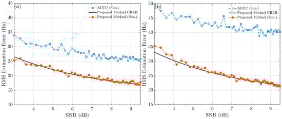
Figure 4. Root Mean Square Error (RMSE) comparison versus SNR (dB). The plots illustrate: the simulated RMSE of the ACCC method (dashed blue line with square markers), the theoretical Cramér–Rao Lower Bound (CRLB) for the proposed method (solid black line), and the simulated RMSE of the proposed method (dashed orange line with circular markers). (a) The result of simulation 1; (b) The result of simulation 2.

In the second simulation, the simulated signal incorporates a left AASR of −12.45 dB. Random SAR image signals with varying SNR were designed. Figure 4b illustrates the estimation accuracy results for both methods under different SNR conditions, with the simulated signal exhibiting left-azimuth ambiguity and an AASR of −12.5 dB. Compared with Simulation 1, the estimation accuracy of both methods is degraded in the presence of ambiguous signals. However, the figure shows that the average discrepancy between the ACCC method’s accuracy and the CRLB is approximately 14 Hz, whereas the proposed estimation method’s accuracy approaches the CRLB. The third simulation was designed to investigate the two methods under a constant SNR and varying left AASR. Keeping the SNR at 8 dB and the left AASR ranging from −16 dB to −7 dB, the bias between the Doppler frequency shift estimated by the two methods and the true value was assessed. From the experimental results in Figure 5a, the ACCC method’s estimates deteriorate at high ambiguity ratios, and the estimated Doppler frequency shift bias increases sharply. In contrast, the estimation error of the proposed method remains consistently around 0 Hz. Consequently, the method proposed in this paper demonstrates the ability to maintain a low estimation bias even under high azimuth ambiguity ratios, which is mainly attributed to the accurate modeling of the DPS. For instance, in the third simulation, with an SNR of 7.8 dB and an AASR of −6.85 dB, the established DPS model is shown in Figure 5b. This model partitions the DPS into two distinct components (i.e., the main-lobe signal and the left azimuth ambiguity signal). Therefore, by constructing this model, the actual Doppler frequency shift within the main signal bandwidth can be estimated with relative precision.

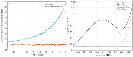
Figure 5. (a) Comparison of the Doppler frequency shift estimation bias between the ACCC method (dashed blue line with square markers) and the proposed method (solid orange line with circular markers) versus different Azimuth Ambiguity-to-Signal Ratios (AASR). (b) Reconstruction of the Power Spectrum Model. This schematic illustrates the partitioning of the Total Signal (solid black line) into the Main Signal Component (dashed blue line), the Ambiguous Component (dashed orange line), and the System Noise (dotted black line) based on the modeled DPS.

For modeling the DPS, it is essential to clarify the rationale for incorporating only first-order azimuth ambiguity in the proposed method. In radar signal processing, the Doppler frequency shift due to the first-order ambiguity is the primary contribution. In contrast, those from higher-order ambiguities are significantly smaller and are often considered negligible, allowing considerable simplification in model computation. To validate the reasonableness of this simplification, a simulation model of the DPS explicitly including fourth-order ambiguity was designed. The simulation parameters were defined as follows: the true Doppler frequency shift in the main lobe signal was set to 0 Hz; the target inducing the right ambiguity exhibited a DPS density 20 dB lower than that of the main signal; the antenna pattern parameters were set according to the Sentinel-1 radar system, with the target velocity ranging from −2 m/s to 2 m/s. The objective was to assess the influence of different orders of ambiguity arising from these varying-velocity targets on the main-lobe signal when using a traditional Doppler radial velocity estimation method. The result is presented in Figure 6, demonstrating that the first-order ambiguity dominates, and the contribution of other ambiguity orders is relatively small and can be effectively ignored.

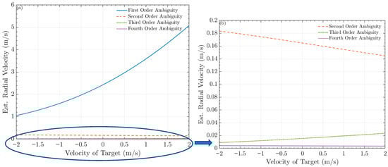
Figure 6. Impact of moving target-induced different order ambiguity in the main signal on Doppler radial velocity estimation: (a) Simulation results of the effects of first-to fourth-order Doppler azimuth ambiguities. (b) Enlarged view of the second- to fourth-order azimuth Doppler ambiguities in (a).

3. The Real Data Experiments and Analysis

3.1. Data Acquisition

3.1.1. Sentinel-1 SAR Data

The Sentinel-1 mission consists of a constellation of two polar-orbiting SAR satellites (Sentinel-1A and Sentinel-1B). Sentinel-1 data are provided in three levels: level-0, which is unfocused raw SAR data; level-1, which includes SLC and ground range detected images; and level-2, which is value-added products derived from the image data. This work is based on Sentinel-1 RAW data (level 0). SM mode acquires data with an 80 km swath and slightly better than 5 m spatial resolution (single look). SM images have a continuous along-track image quality at an approximately constant incidence angle. The centroid frequency of the Sentinel-1 SAR is 5.405 GHz, and the polarization of all acquisitions used is VV and HH polarization.

Level-2 consists of geo-located geophysical products derived from Level-1. Level-2 OCN products for wind, wave, and current applications may contain the following geophysical components derived from SAR data: ocean wind field (OWI), ocean swell spectrum (OSW), and surface radial velocity (RVL). The OWI component is a gridded estimate of wind speed and direction at 10 m above ground level. The RVL component primarily contains the DC (Doppler centroid) and RVL parameters [20]. The spatial resolution of the RVL component is 1 km × 1 km.

3.1.2. HYCOM Data

The global data-assimilative HYCOM product from GOFS 3.1 is run on a 1/12° (0.08°, approximately 8–9 km) tripolar grid with 41 hybrid vertical layers, updated every 3 h. The daily assimilation cycle incorporates altimeter sea-surface height anomaly (SSHA), satellite SST, in situ temperature and salinity profiles, and sea-ice concentration [37]. To compare with SAR radial ocean current, HYCOM surface vector currents are linearly interpolated in time to each Sentinel-1 acquisition, projected onto the radar line-of-sight (LOS), and used as the current-only reference after subtracting the wind-driven radial Doppler component predicted by the CDOP model from both the Sentinel-1 RVL product and our retrieval. Since the native spatial resolutions differ (our retrieval: 0.455 km × 0.575 km; RVL: 1 km × 1 km), both SAR-based products are averaged to the HYCOM native 0.08° grid to reduce scale mismatch and representativeness errors. All analyses are limited to ocean-only pixels after applying a land–sea mask, and all metrics are calculated on an identical set of collocated samples.

3.2. Results and Performance Analysis

In this section, we present two examples to demonstrate the advantages of the proposed method for radial ocean current retrieval. The first example highlights the method’s high resolution, accuracy, and its ability to preserve more textural details of the radial ocean surface current. Conversely, the second example demonstrates the method’s efficacy in eliminating azimuth ambiguity.

3.2.1. Example 1

The first example is an ocean RAW data acquired by Sentinel-1 on 20 May 2023, in the central Indian Ocean, south of the equator. By unpacking raw data to extract echo signals and using imaging parameters, the CSA is applied for imaging. The SLC image used in this example has 19,128 pixels in the Range direction and 57,750 pixels in the Azimuth direction. After completing the previous processing steps for the SAR image, the system’s noise and antenna patterns are estimated. The antenna pattern shape actor b in Equation (5) is estimated to be 1270, and the system noise power density N₀ is 0.4535. The Normalized Radar Cross Section (NRCS) image of the VV polarization is shown in Figure 7a, where ‘Az’ indicates the azimuth direction and ‘Rg’ indicates the range direction. Figure 7b shows the RVL product result at a resolution of 1 km × 1 km, and Figure 7c shows the radial velocity obtained using the proposed method.

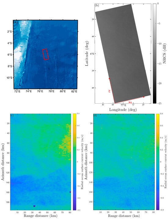
Figure 7. Comparison of radial velocity retrieval results from two methods: (a) Geographic location map of the study area, (b) The SAR NRCS map, (c) The radial ocean surface velocity of the RVL product, (d) The retrieved radial ocean surface velocity using the proposed method.

As shown in Figure 7, the proposed method produces radial ocean current patterns that align with the Sentinel-1 RVL product but have significantly more detailed textures. This enhancement results from the higher effective resolution of our technique. To measure this, we define the following metrics based on the image intensity.

The azimuth (L_az) and range (L_rg) correlation lengths represent the spatial lag $\Delta$ where the normalized autocorrelation functions decay to $1/e$:

$$L_i=\left\{\Delta \left|R_i(\Delta )=R_i(0)/e\right.\right\},i\in \left\{az,rg\right\},$$

(26)

where R_az and R_rg are the autocorrelation functions in the azimuth and range directions, respectively. The equivalent correlation length (L_eq) serves as a unified measure of the effective texture scale:

$$L_{eq}= \sqrt{L_{az}\cdot L_{rg}},$$

(27)

Furthermore, the high-frequency spectral energy ratio (R_HF) quantifies fine-scale details by measuring the proportion of spectral energy above a cutoff wavenumber k₀ within the image power spectrum P(k_x, k_y):

$$R_{HF}={\displaystyle \frac{{\displaystyle \underset{k>k_0}{\iint }P\left(k_x,k_y\right)d{k}_{x}d{k}_y}}{{\displaystyle \iint P\left(k_x,k_y\right)d{k}_{x}d{k}_y}}},$$

(28)

Table 2 presents a quantitative assessment of the spatial-scale characteristics of the retrieved radial ocean surface currents, demonstrating the proposed method’s enhancement in spatial resolution and fine-scale texture. The compelling evidence for fine-scale detail enhancement is the High-Frequency Spectral Energy Ratio. The value obtained by the proposed method (0.101) is more than double that of the Sentinel-1 RVL product (0.048), confirming that an amount of high-wavenumber (fine-scale) energy is successfully retained in the retrieved current. In terms of spatial refinement, the proposed method achieves Azimuth and Range Resolutions of 455 m and 575 m, respectively. This represents a substantial improvement, reducing the original Sentinel-1 RVL resolutions (1000 m and 1000 m) by approximately 54.5% and 42.5%. The physical correlation lengths, measured in meters, show a distinct trend: Azimuth (40,950 m vs. 42,000 m) and Range (3157 m vs. 7950 m). The moderate decrease in Azimuth Correlation Length (2.5%) and the reduction in Range Correlation Length (60.3%) collectively indicate a significant decline in the spatial coherence of the ocean current structures, particularly along the range direction. This collective shortening of correlation lengths is direct proof of the method’s capability to resolve finer-scale features. Consequently, the Equivalent Correlation Length (ECL), also measured in meters, is substantially reduced by 35.8% for the proposed method (16,093.75 m vs. 25,099.8 m). This decrease indicates a reduction in overall structural continuity and an increase in effective statistical noise compared to the Sentinel-1 RVL product. In summary, these metrics demonstrate that the proposed method achieves higher spatial resolution for current retrieval and successfully enhances fine-scale texture details.

Table 2. The assessment of the retrieved method.

Evaluation Metrics	Sentinel-1 RVL Product	The Proposed Method
Azimuth Resolution (m)	1000	455
Range Resolution (m)	1000	575
Azimuth Correlation Length (m)	42,000	40,950
Range Correlation Length (m)	7950	3157
Equivalent Correlation Length (m)	25,099.8	16,093.75
High-Frequency Spectral Energy Ratio	0.048	0.101

Generally, the effectiveness of radial ocean current retrieval from SAR imagery is validated using HF radar data. Unfortunately, there are essentially no corresponding HF radar data covering the Sentinel-1 SM mode data coverage area. As a compromise, the HYCOM model data were chosen to complete the effectiveness validation. The HYCOM vector currents were temporally interpolated to match the SAR observation times and then projected onto the radar LOS direction. To isolate the intrinsic ocean-current signal, the wind-induced Doppler frequency shift component predicted by the CDOP model was subtracted from both the Sentinel-1 RVL product and the proposed retrieval, yielding wind-corrected radial velocities. Considering the difference in native spatial resolutions (proposed method: A_z 0.455 km × R_g 0.575 km; Sentinel-1 RVL product: A_z 1 km × R_g 1 km), both datasets were down-sampled to the native HYCOM grid before comparison, thereby minimizing scale mismatch and representativeness errors. All metrics were computed over the same set of collocated samples. Figure 8a,b presents a visual comparison between the HYCOM reference data (x-axis) and the two retrieval results: the Sentinel-1 RVL product (left column) and the proposed method (right column). The data points are color-coded according to their normalized local density, while the dashed line denotes the ideal 45° reference. In the experiment (N = 398), the Sentinel-1 RVL product yielded a mean absolute error (MAE) of 0.123 m s⁻¹, a root mean squared error (RMSE) of 0.153 m s⁻¹, and a correlation coefficient (R) of 0.590. In contrast, the proposed method achieved an MAE of 0.083 m s⁻¹, an RMSE of 0.100 m s⁻¹, and R = 0.705, corresponding to improvements of 32.1% and 34.3% in MAE and RMSE, respectively. The correlation coefficient was not very high, which is reasonable given that the HYCOM data is model output, not measured data, and is output every 3 h, so the data used were obtained through temporal interpolation. Furthermore, the relatively low resolution of the HYCOM data contributes to the observed discrepancies between the two datasets. The paired boxplots of absolute errors (Figure 8c) further confirm a systematic shift toward lower magnitudes, with the proposed method consistently exhibiting lower MAE values. These consistent and quantifiable improvements demonstrate that, relative to the HYCOM reference, the proposed approach provides a more accurate and reliable estimation of ocean surface radial velocities than the Sentinel-1 RVL product.

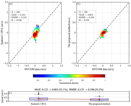
Figure 8. Accuracy comparison against HYCOM for experiment data sets. Panels (a–c) correspond to set Exp.1 (N = 398). Scatter plots (a,b) compare HYCOM data (x-axis) with Sentinel-1 RVL (left column) and the proposed method (right column); data points are colored by normalized local point density. The dashed line is a fixed 45° reference (y = x when axis units and scales match). Insets report N, MAE, R, and RMSE (m s⁻¹). Paired boxplots (c) summarize absolute errors, with red dots marking the MAE. Compared with RVL, the proposed method reduces MAE by 32.1% and RMSE by 34.3% in this experiment (MAE 0.123 → 0.083; RMSE 0.153 → 0.100; R 0.590 → 0.705). All metrics are computed against temporally interpolated HYCOM data to the observation times.

3.2.2. Example 2

To demonstrate the proposed method’s capability to eliminate azimuth ambiguities, SAR imagery exhibiting Doppler azimuth ambiguities was identified and used in an experimental case study. The second example utilized SAR data acquired by the Sentinel-1 satellite on 23 April 2023, in the Seychelles Islands. The SLC image used in this example has 21,186 pixels in the range direction and 46,774 pixels in the azimuth direction. Figure 9a is the geographic location map of the study area. Figure 9b shows the NRCS image of the HH band, which includes an island and a low scattering region. Figure 9c shows the RVL results, and Figure 9d shows the radial ocean current results retrieved using the method proposed in this paper. Significant discrepancies are observed between Figure 9c and Figure 9d at the study points labeled P₁ and P₂ (corresponding to the red-dashed regions marked 1 and 2, respectively).

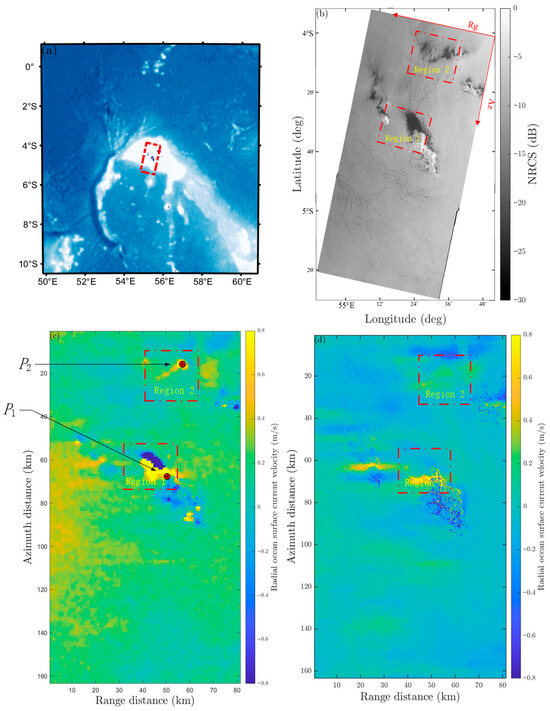
Figure 9. Comparison of radial velocity retrieval results from two methods: (a) Geographic location map of the study area, (b) SAR NRCS map, (c) The radial ocean surface velocity of the RVL product, (d) The radial ocean surface velocity retrieved using the proposed method.

According to the preceding theory, the local DPS shown in Figure 10, corresponding to the two locations selected in Figure 9 for this experiment, contains ambiguous signal components, and the energy contributions from the left and right ambiguous signals are unequal. The analysis for P₁ and P₂ proceeds as follows:

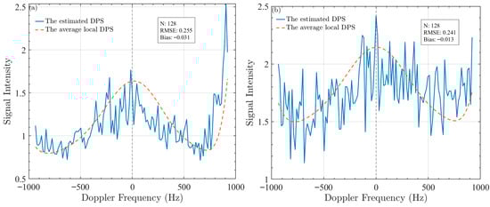
Figure 10. (a) The local DPS and the fitting results of the proposed method at point P₁. (b) The local DPS and the fitting results of the proposed method at point P₂.

Location P₁: Figure 10a presents the local DPS at location P₁ and the corresponding modeling results (Fitting results: RMSE = 0.255, Bias = −0.031) based on the parameters estimated by the proposed method. The local DPS at P₁ is strongly influenced by leftward ambiguity on its right. The SAR image confirms that the selected area is a low-scattering region. According to SAR imaging principles, the Doppler frequency shift in low-scattering areas is susceptible to azimuth ambiguity from strong targets, and the nearby island is such a target. From Equation (7), the azimuth ambiguous signal offset $D_{azi}$ at point P₁ corresponds to the azimuth ambiguity distance observed in the retrieved radial ocean current velocity map. This ambiguity distance can be calibrated to the island’s location, confirming that the strong ambiguous signal is due to the left-azimuth ambiguity generated by the island. Based on the fitting indicators, the strong agreement between the proposed model and the local DPS data suggests that the method is accurate and trustworthy. Crucially, the current value from the RVL product at this point exceeds 1.5 m/s, showing a significant difference compared to the nearby radial ocean current velocity. In contrast, the estimated value from the proposed method is close to 0.15 m/s, a result achieved after eliminating the influence of azimuth ambiguity.

Location P₂: Figure 10b presents the modeling result of the proposed method on the local DPS at point P₂, based on the estimated parameters (Fitting results: RMSE = 0.241, Bias = −0.013). Based on the achieved fitting metrics, the results are highly satisfactory. The SAR image indicates that this position is located within a low-backscatter area, where the left-azimuth ambiguity has a more pronounced effect on the right-hand-side morphology of the local DPS. Further analysis reveals that the NRCS is stronger at the azimuth ambiguity distances ($D_{azi}$) on both sides of the SAR image compared to the location itself. This suggests that ambiguity energy is folding into the DPS of the selected region. At location P₂, the estimated value derived from the RVL product registers 1.2 m/s, which is notably higher than the surrounding areas. Conversely, the estimate derived from the proposed methodology, after mitigation of azimuth ambiguity effects, approximates 0 m/s, thereby achieving substantial consistency with the surrounding regional values.

Analysis of the results at locations P₁ and P₂ demonstrates that the azimuth Doppler ambiguities observed in the Sentinel-1 RVL product (Figure 9a) have been effectively eliminated in Figure 9d. This validates the proposed method’s capability to suppress strong ambiguity signals. It is worth noting that while this visual improvement is most striking for high-contrast point targets (like P₁ and P₂), the underlying suppression mechanism applies equally to the distributed ocean surface. In these distributed regions, ambiguity removal manifests as a general reduction in background noise, thereby improving the overall quality of the retrieved radial ocean current velocity.

4. Discussion

4.1. Accuracy Improvement and Model Consistency

The proposed MAP estimation method offers better accuracy than traditional algorithms. By directly modeling the local DPS, our approach effectively minimizes the estimation variance. The validation against HYCOM data confirms this robustness, showing 34.3% reductions in RMSE and 32.1% in MAE compared to the standard Sentinel-1 RVL product. The increase in the correlation coefficient (from 0.590 to 0.705) indicates that our retrieved currents align much better with the actual ocean circulation patterns.

4.2. High-Resolution Capabilities

A key contribution of this work is the ability to resolve fine-scale ocean features. While standard products often smooth out details to reduce noise, our method maintains a high resolution (approx. 500 m). This is quantitatively proven by the High-Frequency Spectral Energy Ratio, which is more than double that of the RVL product (0.101 vs. 0.048). This enhancement allows for the effective detection of sub-mesoscale dynamics, such as small eddies, which are crucial for detailed oceanographic studies.

4.3. Effective Suppression of Azimuth Ambiguity

Azimuth ambiguity is a significant source of error in coastal SAR observations. Our real-data experiment in the Seychelles clearly demonstrated that the proposed method can suppress ambiguous signals arising from strong scattering targets. Unlike the RVL product, which showed anomalous velocities (>1.5 m/s) due to aliasing, our method successfully corrected these errors, yielding realistic current values (~0 m/s). This proves the method’s reliability for monitoring complex coastal environments.

5. Conclusions

This study proposes and validates a method for retrieving radial ocean current velocity from SAR imagery by employing a Local DPS model within a MAP estimation framework. The method is designed to systematically address two critical limitations inherent in traditional algorithms: insufficient accuracy in Doppler frequency shift estimation and susceptibility to errors induced by azimuth ambiguity. The theoretical superiority of the proposed approach was first confirmed through comprehensive simulation experiments. Results demonstrate that across varying SNR and AASR conditions, the estimation accuracy consistently approaches the CRLB, exhibiting precision superior to that of the traditional ACCC method. This performance advantage was substantiated by processing real Sentinel-1 SM mode data. First, comparisons of the retrieved current velocity with the official Level-2 RVL product and HYCOM model data validated the method’s effectiveness, demonstrating significant reductions in MAE and RMSE of 32.1% and 34.3%, respectively. Concurrently, quantitative metrics confirmed the method’s dual capability of achieving high spatial resolution while preserving the fine-scale textural details of radial ocean currents. Second, the method successfully corrected velocity anomalies caused by azimuth ambiguities arising from strong scatterers (e.g., islands) and high-NRCS regions, thereby explicitly verifying its ability to effectively suppress azimuth ambiguities. Consequently, the proposed algorithm provides a reliable solution for more precise radial ocean current velocity estimates. Given that this research primarily focused on SM mode data, a crucial direction for future work is to extend the method’s application to wider-swath Interferometric Wide Swath (IW) and Extra Wide Swath (EW) mode data. This extension will facilitate direct comparisons with denser HF radar observations in coastal regions, enabling feedback-driven algorithm refinement and further enhancing the accuracy of SAR-derived radial velocities.

References

- Jackson, C.R.; John, R.A. Synthetic Aperture Radar: Marine User’s Manual; National Environmental Satellite: Suitland, MD, USA, 2004.
- Buck, C. An extension to the wide swath ocean altimeter concept. In Proceedings of the 2005 IEEE International Geoscience and Remote Sensing Symposium, Seoul, Republic of Korea, 25–29 July 2005; Volume 8, pp. 5436–5439. [Google Scholar] [CrossRef]
- Quilfen, Y.; Chapron, B. Ocean surface wave-current signatures from satellite altimeter measurements. Geophy. Res. Lett. 2019, 46, 253–261. [Google Scholar] [CrossRef]
- Danilo, C.; Chapron, B.; Mouche, A.; Garello, R.; Collard, F. Comparisons between HF radar and SAR current measurements in the Iroise Sea. In Proceedings of the OCEANS 2007-Europe, Aberdeen, UK, 18–21 June 2007; Volume 6, pp. 1–5. [Google Scholar] [CrossRef]
- Hansen, M.W.; Collard, F.; Dagestad, K.F.; Johannessen, J.A.; Fabry, P.; Chapron, B. Retrieval of sea surface range velocities from Envisat ASAR Doppler centroid measurements. IEEE Trans. Geosci. Remote Sens. 2011, 49, 3582–3592. [Google Scholar] [CrossRef]
- Chapron, B.; Collard, F.; Ardhuin, F. Direct measurements of ocean surface velocity from space: Interpretation and validation. J. Geophys. Res. Oceans 2005, 110, C07008. [Google Scholar] [CrossRef]
- Romeiser, R.; Suchandt, S.; Runge, H.; Steinbrecher, U.; Grunler, S. First analysis of TerraSAR-X along-track InSAR-derived current fields. IEEE Trans. Geosci. Remote Sens. 2009, 48, 820–829. [Google Scholar] [CrossRef]
- Krug, M.; Mouche, A.; Collard, F.; Johannessen, J.A.; Chapron, B. Mapping the Agulhas Current from space: An assessment of ASAR surface current velocities. J. Geophys. Res. Oceans 2010, 115, C10026. [Google Scholar] [CrossRef]
- Moiseev, A.; Johnsen, H.; Hansen, M.W.; Johannessen, J.A. Evaluation of radial ocean surface currents derived from Sentinel-1 IW Doppler shift using coastal radar and Lagrangian surface drifter observations. J. Geophys. Res. Oceans 2020, 125, e2019JC015743. [Google Scholar] [CrossRef]
- Essen, H.H.; Gurgel, K.W.; Schlick, T. On the accuracy of current measurements by means of HF radar. IEEE J. Ocean. Eng. 2002, 25, 472–480. [Google Scholar] [CrossRef]
- Goldstein, R.M.; Zebker, H.A.; Barnett, T.P. Remote sensing of ocean currents. Science 1989, 246, 1282–1285. [Google Scholar] [CrossRef]
- Gabriel, A.K.; Goldstein, R.M.; Zebker, H.A. Mapping small elevation changes over large areas: Differential radar interferometry. J. Geophys. Res. Solid Earth 1989, 94, 9183–9191. [Google Scholar] [CrossRef]
- Romeiser, R.; Runge, H.; Suchandt, S.; Kahle, R.; Rossi, C.; Bell, P.S. Quality assessment of surface current fields from TerraSAR-X and TanDEM-X along-track interferometry and Doppler centroid analysis. IEEE Trans. Geosci. Remote Sens. 2013, 52, 2759–2772. [Google Scholar] [CrossRef]
- Romeiser, R.; Breit, H.; Eineder, M.; Runge, H.; Flament, P.; De Jong, K.; Vogelzang, J. Current measurements by SAR along-track interferometry from a space shuttle. IEEE Trans. Geosci. Remote Sens. 2005, 43, 2315–2324. [Google Scholar] [CrossRef]
- Yuan, X.; Wang, J.; Han, B.; Wang, X. Study on the elimination method of wind field influence in retrieving a sea surface current field. Sensors 2022, 22, 8781. [Google Scholar] [CrossRef]
- Goldstein, R.M.; Zebker, H.A. Interferometric radar measurement of ocean surface currents. Nature 1987, 328, 707–709. [Google Scholar] [CrossRef]
- Wollstadt, S.; López-Dekker, P.; De Zan, F.; Younis, M. Design principles and considerations for spaceborne ATI SAR-based observations of ocean surface velocity vectors. IEEE Trans. Geosci. Remote Sens. 2017, 55, 4500–4519. [Google Scholar] [CrossRef]
- Shuchman, R.A.; Rufenach, C.L.; Gonzalez, F.I.; Klooster, A. The feasibility of measurement of ocean surface currents using synthetic aperture radar. In Proceedings of the Thirteenth International Symposium on Remote Sensing of the Environment, Ann Arbor, MI, USA, 23–27 April 1979; Volume 4. [Google Scholar]
- Hutt, D.; Stockhausen, J.; Osler, J.; Mosher, D. Capability of Radarsat-1 for estimation of ocean surface current on the Scotian Shelf. In Proceedings of the IEEE International Symposium on Geoscience and Remote Sensing, Toronto, ON, Canada, 24–28 June 2002; Volume 4, pp. 2135–2137. [Google Scholar] [CrossRef]
- Bourbigot, M.; Johnsen, H.; Piantanida, R.; Hajduch, G.; Poullaouec, J. Sentinel-1 Product Definition. 2016, ESA Unclassified–For Official Use. Available online: https://sentiwiki.copernicus.eu/__attachments/1673968/S1-RS-MDA-52-7441%20-%20Sentinel-1%20Product%20Specification%202023%20-%203.14.1.pdf (accessed on 18 February 2021).
- Renga, A.; Moccia, A. Use of Doppler parameters for ship velocity computation in SAR images. IEEE Trans. Geosci. Remote Sens. 2016, 54, 3995–4011. [Google Scholar] [CrossRef]
- Bamler, R. Doppler frequency estimation and the Cramer-Rao bound. IEEE Trans. Geosci. Remote Sens. 1991, 29, 385–390. [Google Scholar] [CrossRef]
- Johnsen, H.; Nilsen, V.; Engen, G.; Mouche, A.A.; Collard, F. Ocean doppler anomaly and ocean surface current from Sentinel 1 tops mode. In Proceedings of the 2016 IEEE International Geoscience and Remote Sensing Symposium, Beijing, China, 10–15 July 2016; Volume 7, pp. 3993–3996. [Google Scholar] [CrossRef]
- Moiseev, A.; Johannessen, J.A.; Johnsen, H. Towards retrieving reliable ocean surface currents in the coastal zone from the Sentinel-1 Doppler shift observations. J. Geophys. Res. Oceans 2022, 127, e2021JC018201. [Google Scholar] [CrossRef]
- Madsen, S.N. Estimating the Doppler centroid of SAR data. IEEE Trans. Aerosp. Electron. Syst. 2002, 25, 134–140. [Google Scholar] [CrossRef]
- Engen, G.; Johnsen, H.; Larsen, Y. Sentinel-1 geophysical doppler product-performance and application. In Proceedings of the EUSAR 2014: 10th European Conference on Synthetic Aperture Radar, Berlin, Germany, 3–5 June 2014; pp. 1–4. [Google Scholar]
- Villano, M.; Krieger, G. Spectral-based estimation of the local azimuth ambiguity-to-signal ratio in SAR images. IEEE Trans. Geosci. Remote Sens. 2013, 52, 2304–2313. [Google Scholar] [CrossRef]
- Sun, K.; Diao, L.; Zhao, Y.; Zhao, W.; Xu, Y.; Chong, J. Impact of SAR azimuth ambiguities on Doppler velocity estimation performance: Modeling and analysis. Remote Sens. 2023, 15, 1198. [Google Scholar] [CrossRef]
- Azouz, A.; Fouad, M.; ELbohy, A.; Abdalla, A.; Mashaly, A. SAR image formation scheme implementation and endorsement sprouting from Level-0 data decoding. Egypt. J. Remote Sens. Space Sci. 2023, 26, 253–263. [Google Scholar] [CrossRef]
- Raney, R.K.; Runge, H.; Bamler, R.; Cumming, I.G.; Wong, F.H. Precision SAR processing using chirp scaling. IEEE Trans. Geosci. Remote Sens. 2002, 32, 786–799. [Google Scholar] [CrossRef]
- Chitroub, S.; Houacine, A.; Sansal, B. Statistical characterisation and modelling of SAR images. Signal Process. 2002, 82, 69–92. [Google Scholar] [CrossRef]
- Oliver, C.; Quegan, S. Understanding Synthetic Aperture Radar Images; SciTech Publishing: Raleigh, NC, USA, 2004. [Google Scholar]
- Meng, H.; Wang, X.; Chong, J.; Wei, X.; Kong, W. Doppler spectrum-based NRCS estimation method for low-scattering areas in ocean SAR images. Remote Sens. 2017, 9, 219. [Google Scholar] [CrossRef]
- Ocean Data Lab. S-1 RVL DIL4: Algorithm Description Document. ESRIN: ESA. 2015. Available online: https://sentiwiki.copernicus.eu/__attachments/1673968/S1-TN-NRT-53-0658%20-%20Sentinel-1%20doppler%20and%20Ocean%20Radial%20Velocity%20(RVL)%20ATBD%202024%20-%201.7.pdf?inst-v=b88bce31-6a7b-41d2-99d5-181e8ab7e5d5 (accessed on 15 July 2015).
- Mouche, A.A.; Collard, F.; Chapron, B.; Dagestad, K.F.; Guitton, G.; Johannessen, J.A.; Hansen, M.W. On the use of Doppler shift for sea surface wind retrieval from SAR. IEEE Trans. Geosci. Remote Sens. 2012, 50, 2901–2909. [Google Scholar] [CrossRef]
- Meng, H.; Wang, X.; Chong, J. An Azimuth antenna pattern estimation method based on Doppler spectrum in SAR ocean images. Sensors 2018, 18, 1081. [Google Scholar] [CrossRef]
- Chassignet, E.P.; Hurlburt, H.E.; Smedstad, O.M.; Halliwell, G.R.; Hogan, P.J.; Wallcraft, A.J.; Bleck, R. The HYCOM (hybrid coordinate ocean model) data assimilative system. J. Marine Syst. 2007, 65, 60–83. [Google Scholar] [CrossRef]
Disclaimer/Publisher’s Note: The statements, opinions and data contained in all publications are solely those of the individual author(s) and contributor(s) and not of MDPI and/or the editor(s). MDPI and/or the editor(s) disclaim responsibility for any injury to people or property resulting from any ideas, methods, instructions or products referred to in the content. |
© 2025 by the authors. Licensee MDPI, Basel, Switzerland. This article is an open access article distributed under the terms and conditions of the Creative Commons Attribution (CC BY) license (https://creativecommons.org/licenses/by/4.0/).