Displacement Time Series Forecasting Using Sentinel-1 SBAS-InSAR Results in a Mining Subsidence Case Study—Evaluation of Machine Learning and Deep Learning Methods

Highlights

What are the main findings?

• Data-driven models, including deep neural networks, successfully captured the temporal course of mining-induced ground subsidence based on SBAS-InSAR time series.
• Model performance varied across different forecast horizons and across the study area, with local outliers and heterogeneous accuracy measures.

What is the implication of the main finding?

• Integrating SBAS-InSAR observations with machine learning models can provide a framework for continuous ground deformation monitoring and prediction.
• A comprehensive assessment of models’ accuracy, in both spatial and temporal domains, is essential for improving model reliability in risk assessment and early-warning scenarios.

Abstract

With an abundance of data provided by satellite-based measurements, such as Synthetic Aperture Radar Interferometry (InSAR) or the Global Navigation Satellite System (GNSS), an interest has grown in training highly complex data-driven models for geophysical applications, including displacement modeling. These methods, including machine learning (ML) and deep learning (DL) algorithms, represent a new approach to forecasting ground surface displacements. Yet, the effectiveness of such methods, including their generalization capabilities and performance on non-linear data, remains underexplored. This paper examines the performance of various data-driven algorithms, including regression models and deep neural networks, in predicting mining-induced subsidence. Ground surface displacement data obtained from the Small Baseline Subset (SBAS) InSAR were used as time series samples for training and validation. ML and DL models were evaluated over varying forecast horizons. The results show that data-driven approaches can effectively model InSAR-derived ground subsidence in mining areas. Deep learning models outperform other ML-based models, indicating that increased model complexity can lead to better forecasting accuracy. Nevertheless, it is shown that careful examination of performance metrics and forecast errors in the spatial domain is essential for appropriate model evaluation. The findings demonstrate that combining SBAS-InSAR measurements with data-driven modeling offers a promising direction for developing automated systems for monitoring and forecasting mining-induced ground deformation.

1. Introduction

Underground mining operations generate complex influences on the ground surface, including ground subsidence, that can pose a significant risk to buildings and technical infrastructure. Managing risks posed by underground mining requires accurate forecasting of ground displacements. While a variety of methods and techniques for subsidence prediction have been developed around the world, their individual applicability often depends on locally specific constraints, such as different geological and operational contexts [1].

Methods for mining subsidence monitoring include Global Navigation Satellite System (GNSS) measurements [2], precise leveling [3], Synthetic Aperture Radar (SAR) Interferometry (InSAR) [4], and unmanned aerial vehicle (UAV) photogrammetry [5]. Precise leveling is often the preferred method, owing to high accuracy and extensive experience of mining surveyors in mining area protection. The increasing availability of high-resolution SAR data, particularly from satellite missions such as Copernicus Sentinel-1, presents InSAR as a complementary monitoring tool for mining subsidence studies [6].

In the context of subsidence forecasting, traditional empirical methods, like the Budryk–Knothe approach [7] or the probability integral method (PIM) [8], remain standard practice in numerous mining areas [9,10]. Other approaches include analytical methods [11,12], stochastic modeling [13], methods applying continuous rock mass mechanics [14], and numerical modeling [15]. Each method comes with certain limitations, e.g., numerical methods and rock mechanics models require an extensive knowledge of the modeled rock mass to provide a solution. Empirical methods, while favored by their simplicity, are often confined locally, requiring certain adjustments in different mining areas. Developments in methods based on data analysis, such as machine learning (ML), have introduced a new group of data-driven approaches for subsidence prediction. Using a machine learning approach, ground subsidence is modeled by an algorithm that automatically learns internal relationships and patterns from data without explicit programming. Deep learning (DL) is a subfield of machine learning that uses deep neural networks (DNNs), characterized by multiple hidden layers, to model complex and non-linear relationships in the observed data. In this paper, for the purpose of comparative study, the term machine learning (ML) is specifically applied to denote the non-neural network-based algorithms, while deep learning (DL) is used to describe DNN-based architectures.

ML and DL methods have been applied in surface displacement prediction, including various algorithms such as support vector machines (SVM) [16] and random forest regression (RFR) [17], as well as deep neural networks (DNNs) [18]. An emerging paradigm, including integrating machine learning approaches with time series data for forecasting time series of surface displacements, is an active field of research that could significantly enhance displacement prediction capabilities. These data-driven approaches utilize historical displacement data for model training, beginning with long-established statistical methods like autoregressive modeling and exponential smoothing [19,20]. However, traditional approaches can struggle with non-linear, compound nature of ground deformation processes, while ML methods excel at modeling complex non-linear relationships. Recent studies explored various ML algorithms [19], compared traditional approaches with more complex ML and DL methods [20], and applied novel neural network architectures like long short-term memory (LSTM) [21] or Transformers [22,23] to displacement time series forecasting. Applications of data-driven displacement forecasting also include landslide displacement prediction [24], mining subsidence studies [19,21], and tunnel-induced settlement inspection [25].

The rise of data-driven methods enforced an increased demand for quality time series data for training ML and DL algorithms. With high temporal and spatial resolution, InSAR can provide insight into various geophysical processes. Short-term displacement monitoring using single-pair differential interferometry (DInSAR) proved to be valuable for understanding mining subsidence [26]. Time-series-based InSAR methods are of increasing value for studying mining-induced displacements, supplying researchers and surveyors with regularly delivered, high-resolution data on deformation processes manifesting on the surface [27]. Among the time series InSAR approaches, the Persistent Scatterer (PS) [28,29] and the Small Baseline Subset (SBAS, SBInSAR) [30,31,32] are the two most popular methods for subsidence monitoring.

Despite growing interest in applying machine learning to ground displacement forecasting, several issues are overlooked or require further consideration. Recurrent neural networks (RNNs), particularly the long short-term memory (LSTM) architecture, have emerged as the predominant architecture in displacement time series forecasting thanks to integrated support for sequential data processing [33]. This has often led to a focus on studying novel, more complex neural network architectures, without prior benchmarking with simpler statistical and machine learning algorithms.

With machine learning excelling in processing large quantities of data, an important property is the ability to parse multiple time series from different locations. Geomechanical processes may lead to various kinds of surface deformation, with spatially heterogeneous magnitudes and temporal characteristics. An effective displacement forecasting model should, therefore, consider spatial heterogeneity in the time series data, or be robust against errors and biases associated with these discrepancies. This is not always the case, as traditional forecasting methods create local models on individual time series. On the contrary, machine learning can utilize external information from other time series, providing global forecasting models with broader generalization and scaling capabilities.

Mining displacement forecasts can have a significant impact on decision making; therefore, a robust forecasting strategy needs to be adopted and evaluated. Both short- and long-term forecasting strategies can be considered for operational planning and to mitigate impacts on the surface. Short-term forecasting can supply a prediction system with frequent data updates, enabling anomaly detection and early warning systems. On the other hand, long-term forecasting can provide a more general outlook on the observed and modeled phenomenon, facilitating the planning and coordination processes.

To address the aforementioned challenges and issues, this study proposes a methodological framework for mining subsidence time series forecasting. InSAR time series are used for deploying a number of forecasting models, considering the effectiveness of traditional statistical modeling and machine learning models, as well as novel deep learning architectures. Robustness of global models to spatial heterogeneity is examined through accuracy measures and error maps, and a temporal validation procedure is applied to study the impact of forecast horizon length on model performance. The objective of the study is to investigate time series forecasting models trained on InSAR surface subsidence data in a data-driven approach. Research was conducted on a subsidence trough within a copper ore mining area in southwest Poland.

2. Materials and Methods

2.1. Study Area

The Legnica-Głogów Copper District (LGCD) is an industrial complex located in southwest Poland, in Lower Silesian Voivodeship (Figure 1). The mining area, operated by KGHM Polska Miedź S.A. (Lubin, Poland), covers approximately 492 square kilometers. The LGCD is considered one of the world’s main sources of copper ore. Mining operations, carried out since the 1960s, have had a significant impact on the region’s development [34].

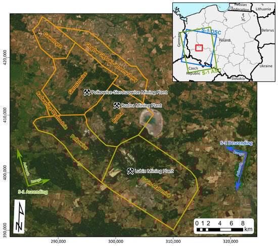
Figure 1. Location of the study area, marked on the inset map of Poland in the top-right corner with a red rectangle. Spatial coverage of Sentinel-1 ascending and descending frames used in the study is highlighted in green and blue, respectively, and the corresponding range vectors have been added to the map. Mining areas are highlighted in orange. Basemap imagery source: ESRI World Imagery. Map coordinate system: PL-1992 (EPSG:2180).

The copper ore deposits of the LGCD feature sedimentary formations within the Fore-Sudetic Monocline, consisting of Permian and Triassic sedimentary rocks, incline slightly towards the northeast. The ore body dips monoclinally at a depth from few hundred meters to 1500 m. The Permian and Triassic formations are covered by Tertiary and Quaternary sediments. The copper-bearing deposits include the white and white–gray Rotliegendes and Zechstein sandstones, as well as copper-bearing Zechstein shales and dolomites. The average bed thickness is around 4 m and varies locally. The deposit is intersected by numerous tectonic faults, further complicating the extraction conditions [34]. Currently, the extraction is carried out in three underground mining plants: Lubin, Rudna, and Polkowice-Sieroszowice (Figure 1).

Mining works in the LGCD are carried out using a room-and-pillar method, with different methods of void fill, depending on geological and mining conditions. Over 45 variants of the method were developed depending on local geological conditions, to optimize both safety and production efficiency [35]. Application of the room-and-pillar method results in a more gentle character of surface subsidence owing to the gradual deterioration of technological pillars.

Surface subsidence monitoring in the LGCD includes multiple complementary approaches, incorporating GNSS measurements [36] and conventional leveling measurements carried out by the mining company. Recent studies employing Copernicus Sentinel-1 SAR data revealed that interferometric SAR effectively captures mining-induced subsidence patterns, achieving measurements with centimeter-level accuracy [29,37,38].

2.2. InSAR Data Processing

Displacement time series derived from SAR interferometry were used in this study. Sentinel-1 SAR Single-Look Complex SLC images from between May 2016 and October 2020 were downloaded from the Alaska Satellite Facility (ASF) archive (https://asf.alaska.edu (accessed on 1 July 2025)), and processed using the DInSAR approach to obtain a set of unwrapped differential interferograms, which were then processed with the SBAS method.

Sentinel-1A/B SAR data from two acquisition orbits (ascending No. 73 and descending No. 22) were considered to facilitate the estimation of vertical displacement time series. Detailed information on the acquired Sentinel-1 data is shown in Table 1. Differential interferograms were created using the InSAR Scientific Computing Environment (ISCE2) software (version 2.6.3) [39]. Precise orbits and enhanced spectral diversity (ESD) were used during image coregistration to meet the required azimuth misregistration accuracy. The Shuttle Radar Topography Mission (SRTM) 1-arc second digital elevation model (DEM) was applied for topographic phase removal in the DInSAR processing [40]. To ensure the quality of the displacement time series after SBAS inversion, only interferograms with a temporal threshold of 50 days and a perpendicular baseline of maximum 150 m were considered in further analysis. Interferograms were multilooked (with 10 looks in range and 2 in azimuth) and filtered using the power spectrum method [41] for noise reduction. Phase unwrapping was performed using the SNAPHU algorithm [42].

Table 1. Information on Sentinel-1 SAR data used for generating interferograms in the SBAS analysis.

Flight Direction	Path No.	Start Date *	End Date	Number of Scenes
Ascending	73	20 May 2016	26 October 2020	278
Descending	22	17 May 2016	23 October 2020	257

* Sentinel-1B data available since 2 October 2016.

Line of sight (LOS) displacement time series were obtained through SBAS inversion of the small baseline interferogram stack, using the MintPy (Miami INsar Time series software in Python) software package (version 1.6.1) [43]. Prior to SBAS inversion, tropospheric correction was estimated following the GACOS approach [44] and applied to interferograms to minimize the impact of tropospheric delay on the displacement time series [37]. Time series results were masked using a temporal coherence threshold (min. 0.7) to ensure the quality of results.

Vertical displacement time series were estimated using the two independent LOS datasets, under an assumption that no displacement is detected in the north–south direction, given the near-polar orbits of the Sentinel-1 satellites and negligible sensitivity to this displacement component [45]. Given the two LOS measurements, the geometric relationship with the vertical and horizontal (east–west) components is given by [46]:

$$\left[\begin{array}{c}{d}_{LOS}^{asc}\\ d_{LOS}^{dsc}\end{array}\right]=\left[\begin{array}{cc}cos{\theta }_{asc}& {\displaystyle \frac{sin{\theta }_{asc}}{cos\Delta \alpha }}\\ cos{\theta }_{dsc}& sin{\theta }_{dsc}\end{array}\right]\left[\begin{array}{c}{d}_V\\ d_{H_{E-W}}\end{array}\right],$$

(1)

where $d_{LOS}^{asc}$ and $d_{LOS}^{dsc}$ are the LOS displacement values from the ascending and descending orbits, respectively; ${\theta }_{asc}$ and ${\theta }_{dsc}$ are incidence angle values for the ascending and descending acquisition, respectively; $\Delta \alpha$ is the difference in the heading angles of the respective LOS acquisitions; and $d_V$ and $d_{H_{E-W}}$ are the vertical and horizontal (E–W) displacement components. Spatial resampling to a common grid with a 30 m spatial resolution was applied to merge the LOS datasets and solve for the displacement components. Furthermore, an assumption on the temporal origin of the displacement data was needed, as the time series are shifted with respect to one another by 3 days, owing to the acquisition strategy of respective ascending and descending orbital paths. The demonstrated methodological approach for vertical displacement estimation corresponds to approaches applied in other studies and monitoring systems, e.g., in the European Ground Motion Service (EGMS) [47]. While mining subsidence is of interest in this paper, only the vertical displacement time series were subject to forecasting.

2.3. Time Series Forecasting Model Development

2.3.1. Forecasting Strategy

The models in this study were developed as univariate, multi-step forecasting models, trained using only ground displacement time series data obtained with the SBAS InSAR method. No additional covariates were considered for prediction. The data-driven models were evaluated in a multi-step forecasting scenario with different lengths of the forecast horizon. Five different forecast horizons were considered when determining the forecasting strategy to evaluate different models’ performance in short- and long-term prediction. Here, 5-, 10-, 20-, 30-, and 60-step horizons were considered, corresponding to 30-day (approx. 1 month), 60-day (approx. 2 months), 120-day (approx. 4 months), 180-day (approx. 6 months), and 360-day (approx. 1 year) forecasts, respectively. The selected time intervals represent different hypothetical horizons required by operational decision making, including short-term prediction (30, 60 days) for immediate and short-term deformation analysis, and longer-term prediction (120, 180, 360 days) for long-range risk assessment. Including a range of forecast horizons places the evaluated models in a variety of operational scenarios, testing their performance both in an immediate horizon, where temporal correlation between subsequent time steps is high, and in a long-term scenario, where non-linearities and anomalous time series behavior may influence the model’s performance.

2.3.2. Time Series Preprocessing

The dataset derived from SBInSAR results contains time series of ground surface displacements in regularly distributed points covering the study area. A total of 9068 points were collected over the studied subsidence trough (described in detail in the Section 3). Each time series covers the period from 20 May 2016 to 26 October 2020, with a time step interval of 6 days. Missing values (resulting from the absence of SAR acquisitions, including the unavailability of Sentinel-1B data for a part of 2016) were inserted through ordinary linear interpolation, assuming that mining-induced subsidence is a process that is generally continuous and smooth over short intervals, and that linear interpolation should provide a good estimate for the short temporal gaps. As only a small portion of the dataset (approx. 5%) exhibited missing values, the interpolation algorithm was considered to not have an impact on the model training process. Prior to model training, the time series values were rescaled to a [0, 1] range, to ensure consistent training across all models and stabilize training of the neural network models.

In order to prevent data leakage during model training, the time series dataset was divided into training and test subsets, using a random split of 30% for training and validation, and the remaining 70% for testing. Each time series was also divided into input (training) and output (validation) series, depending on the length of the forecast horizon (Table 2). The models were validated and tested using only the output series.

Table 2. Temporal splits into training and testing time series datasets, depending on forecast horizon.

Forecast Horizon	Training Data Period	Testing Data Period
5 time steps	20.05.2016–26.09.2020	26.09.2020–26.10.2020
10 time steps	20.05.2016–27.08.2020	27.08.2020–26.10.2020
20 time steps	20.05.2016–28.06.2020	28.06.2020–26.10.2020
30 time steps	20.05.2016–29.04.2020	29.04.2020–26.10.2020
60 time steps	20.05.2016–01.11.2019	01.11.2019–26.10.2020

2.3.3. Model Development

This study compared six data-driven models, including a Holt–Winters exponential smoothing model as a baseline model for comparing ML- and DL-based approaches. Regarding the ML approaches, a linear regression model with regularization (ElasticNet), as well as two tree-based models, random forest and extreme gradient boosting (XGBoost), were considered. Finally, two neural network (DL) models were examined, including a fully connected model (N-BEATS) and a model with recurrent layers (LSTM).

The exponential smoothing approach is a time series forecasting method that applies a weighted average to past observations for generating predictions, with weights decreasing exponentially for earlier observations. As the displacement time series observed in the study area are mainly characterized by trend with minor seasonal oscillations, the Holt–Winters algorithm was adopted in this study as a baseline, extending the model to account for trend and seasonality in the time series through a number of smoothing parameters (error, trend, seasonality (ETS)) [48]. An AutoETS implementation, which searches for the optimal ETS parameters using the Akaike’s information criterion, was used in this study to identify optimal model parameters for local time series data [49].

A machine-learning-based linear regression model learns the relationships between input past time series values and output future values in a supervised manner. A set of input–output data is created from the time series to train the model, following a moving window approach. The ElasticNet regularized linear regression approach was adopted in the study, combining the L1 and L2 regularization terms of Lasso and Ridge regression methods [50].

Another machine learning method used in the study was the random forest model, which fits a number of decision trees (DTs) to random subsets of the training dataset and averages the subsequent DT results for the final regression prediction. Much like in linear regression, past observations are used as input values to predict future values using regression. The random forest approach was considered due to its ability to capture non-linear relationships in the data [51].

A second tree-based model, the XGBoost method, was considered is this paper as an alternative ensemble learning approach to the random forest method. In this method, decision trees are built sequentially, each focusing on correcting the errors of the previous one (boosting) [52].

A first deep learning architecture considered in this study was the N-BEATS (Neural Basis Expansion Analysis for interpretable Time Series forecasting) model. This neural network, developed specifically for time series forecasting, is composed of blocks of networks with fully connected layers. N-BEATS decomposes the input time series into a set of functions capturing various temporal patterns (e.g., trend, seasonality, cycles) [53]. This architecture was implemented to evaluate the performance of a fully connected neural network with no recurrence or attention weights in mining displacement forecasting.

Due to its frequently reported effectiveness in time series forecasting, particularly in the displacement prediction domain, a recurrent neural network (RNN) architecture was also examined. Following a broad number of applications in previous studies, the LSTM variant was considered in this paper. The LSTM architecture uses memory cells to decide which part of input data is relevant for future predictions, therefore allowing us to capture long-term dependencies and avoid the exploding gradient problem [33].

Model hyperparameters were selected iteratively based on validation performance. Due to the high computational cost of training multiple models in multiple scenarios (considering varying output forecast horizon), a full grid search was not applied. Hyperparameter values selected for the evaluated ML and DL models are shown in Table 3.

Table 3. Hyperparameter values applied to the selected forecasting models.

Model	Hyperparameters
ElasticNet	$\alpha =1.0$, $l1\_ratio=0.6$
Random Forest	$n\_estimators=300$, $max\_depth=10$, $min\_samples\_split=2$
XGBoost	$learning\_rate=0.1$, $n\_estimators=300$, $max\_depth=8$
N-BEATS	$learning\_rate=0.001$, $num\_layers=4$, $hidden\_units=128$, $batch\_size=128$, $n\_epochs=20$
LSTM	$learning\_rate=0.001$, $num\_layers=2$, $hidden\_units=64$, $batch\_size=128$, $n\_epochs=20$

ML and DL models evaluated in the study were employed as global models, trained on multiple time series covering the entire study area. This choice was justified by a spatial and temporal heterogeneity observed in the time series, defined by varying temporal profiles of subsidence across the study area (e.g., various acceleration/deceleration rates), and differences in vertical displacement magnitude and spatial extent across the subsidence zone. A global model, unlike independent local models (used by statistical forecasting methods), is hypothesized to effectively learn these varying patterns by developing a feature space across all training samples. This should allow the model to capture the underlying heterogeneous patterns more effectively by learning from a variety of training examples and scenarios, leading to better generalization capabilities.

3. Results

3.1. Ground Surface Displacements

Application of the SBInSAR time series method on a dataset of unwrapped DInSAR interferograms, together with LOS displacement decomposition, allowed us to obtain a time series of vertical ground surface displacements for the LGCD mining area. Total vertical displacements measured from 20 May 2016 to 26 October 2020, cropped spatially to the extent of the LGCD area, are shown in Figure 2. Temporal coherence masking allowed the removal of time series data with low reliability, located particularly over forest-covered areas and water bodies.

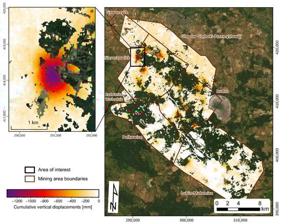
Figure 2. (right) Vertical cumulative displacements for the LGCD mining area, obtained through LOS displacement decomposition of SBAS InSAR results. (left) Subsidence trough located in the Sieroszowice mining area, selected as the case study for the displacement prediction. Basemap imagery source: ESRI World Imagery. Map coordinate system: PL-1992 (EPSG:2180).

A number of subsidence troughs were identified over the area of interest (AOI), which can be attributed to the underground mining operations carried out in the area. The map presented in Figure 2 indicates that subsidence troughs are concentrated mainly in the Sieroszowice mining area (northwest part of the AOI), as well as in the Rudna mining area (central part of the AOI) and the Lubin-Małoszowice mining area (southern part of the AOI). This coincides with the locations of the three mining plants indicated in Figure 1.

Total displacements observed within the subsidence troughs peak up to −1350 mm in the Sieroszowice mining area (indicated on the left map in Figure 2). The majority of troughs’ displacements in the northwestern and central part of the LGCD reached from −1000 mm to −700 mm. Displacement time series exhibit non-linear subsidence trends with varying temporal velocities corresponding to underground extraction activity, as well as occasional rapid accelerations in several subsidence troughs, interrelated with induced mining tremors of high magnitude, owing to seismic activity present in the area [37,54,55,56]. A slight subsidence can also be observed outside the main subsidence zones, mainly over croplands and arable areas. This signal, particularly visible in the northern and northwestern part of the AOI, can most likely be attributed to the fading signal (or phase bias) present when processing multilooked interferograms with short temporal baselines, as reported in numerous publications [57,58].

A subsidence zone in the Sieroszowice mining area (indicated in Figure 2 on the left) exhibits the strongest subsidence signal observed during the study period, reaching −1350 mm. Owing to relatively high temporal coherence in the immediate vicinity, this subsidence zone is clearly visible in the InSAR results, with nearly the entire shape of the subsidence trough outlined. Therefore, this zone was selected as a case study area for training and evaluating the time series forecasting algorithms.

3.2. Displacement Prediction Model Evaluation

Several time series forecasting models, including the traditional Holt–Winters method, machine learning regression algorithms, and deep neural network architectures, were evaluated to assess and compare their ability to predict ground surface displacements. Predictions were performed on a set of time series of displacements, derived from Sentinel-1 SAR SBInSAR results. Models were trained on displacement data from a selected subsidence trough in the Sieroszowice mining area. Model evaluation was conducted on a set of withheld time series observations, following a temporal split to avoid data leakage (described in detail in the Section 2). Time series forecasting models were evaluated in terms of their ability to effectively capture the displacement characteristics, including trends and short-terms fluctuations, considering different forecast horizons. A suite of statistical metrics was used for model evaluation, including the root mean squared error (RMSE), mean absolute error (MAE), and symmetric mean absolute percentage error (sMAPE), calculated with the following formulas:

$$RMSE=\sqrt{{\displaystyle \frac{1}{T}}\sum _{t=1}^T{(y_t-{\widehat{y}}_t)}^2}$$

(2)

$$MAE={\displaystyle \frac{1}{T}}\sum _{t=1}^T|y_t-{\widehat{y}}_t|$$

(3)

$$sMAPE=200\times {\displaystyle \frac{1}{T}}\sum _{t=1}^T{\displaystyle \frac{|y_t-{\widehat{y}}_t|}{|y_t|+|{\widehat{y}}_t|}}$$

(4)

where $y_t$ is the observed value at time step t, ${\widehat{y}}_t$ is the predicted value at time step t, and T is the total number of predicted time steps.

Accuracy metrics were calculated for the individual displacement time series over the study area, using the withheld portions to test the models’ generalization capabilities. Mean performance metrics obtained for all prediction models, considering different forecast horizons, are summarized in Table 4, with the lowest mean metrics for each horizon highlighted in bold. The evaluation metrics (RMSE, MAE, sMAPE) reveal that the Holt–Winters approach and the LSTM neural network achieved the best performance in the study area over different forecast horizons, while the decision-tree-based regression models reported weaker overall performance. A general positive trend can be observed in the mean values of all accuracy metrics with increasing forecast horizon, indicating a growing forecast uncertainty and increasing errors when longer time series are considered.

Table 4. Mean performance metrics of evaluated models, with different forecast horizons considered. Lowest accuracy metrics for each forecast horizon were highlighted in bold.

Model	Metrics	h = 5	h = 10	h = 20	h = 30	h = 60
Holt–Winters	RMSE	6.1	8.3	9.1	11.4	16.6
	MAE	5.5	6.5	7.4	9.4	13.7
	sMAPE	7.3	8.9	10.3	13.5	15.5
ElasticNet	RMSE	6.4	9.8	9.6	10.7	25.6
	MAE	5.6	8.2	7.8	8.8	22.0
	sMAPE	7.3	11.3	10.6	12.0	21.5
Random Forest	RMSE	6.3	10.1	9.7	11.5	27.3
	MAE	5.4	8.4	8.0	9.6	24.2
	sMAPE	6.3	11.5	10.1	11.1	20.0
XGBoost	RMSE	6.8	10.9	12.5	15.5	32.9
	MAE	6.0	9.2	10.6	13.3	29.3
	sMAPE	6.4	10.9	11.1	12.5	18.9
N-BEATS	RMSE	5.4	8.6	10.2	11.6	23.0
	MAE	4.7	7.0	8.3	9.6	19.8
	sMAPE	5.7	9.1	11.0	11.8	18.4
LSTM	RMSE	5.2	8.7	9.4	10.4	20.7
	MAE	4.5	7.1	7.6	8.6	17.3
	sMAPE	5.4	9.2	10.1	11.1	18.9

For short-term forecasting (h = 5), the LSTM model achieved the lowest mean error values across the tested locations, followed by the N-BEATS model and the Holt–Winters model, confirming their capability of predicting displacement time series effectively. The regression models (ElasticNet, random forest, and XGBoost) achieved slightly higher performance metrics, indicating a higher number of forecast errors and a generally lower ability of capturing relevant trends and fluctuations in the time series. This demonstrates that ML-based models, especially tree-based models, exhibit lower performance in short-term interpolation compared to DL-based models. Lower values of the scale-independent sMAPE metric observed for the DL models further indicate that these models generalize better across the entire range of time series characteristics than the simpler ML-based models. This feature is also observed for higher forecast horizons.

Increasing the forecast horizon yields higher performance metrics for all models. For forecast horizons of 10 and 20 time steps, corresponding to 60 and 120 days, the Holt–Winters method achieved performance superior to all other data-driven ML and DL approaches.The performance of the ElasticNet model for h = 10 was slightly worse, even compared to the longer forecast horizon. This might indicate a possible localized effect, where longer output sequences lead to the model better capturing the linear trends and fluctuations in the data during training.

Tests of the 6-months-ahead forecasts (h = 30) further confirmed the capability of ML and DL methods to predict ground surface displacements, with the LSTM and ElasticNet Regression models achieving highest mean performance scores. This implies that models learn from the patterns in the time series to predict future values with higher accuracy compared to traditional forecasting approaches. A higher forecast performance of the linear regression method, compared to shorter forecast horizons, further confirms that this approach, while not being the most suitable predictor for short forecast lengths, is more reliable for longer sequences, better capturing the underlying trends. The lowest metrics of the LSTM model show that a DL-based global model might be more robust and effective in predicting long-term displacements over a range of time series in multiple locations.

Increasing the forecast horizon to 60 time steps, corresponding to 360 days (approx. 1 year), showed that the data-driven approaches failed to contest with traditional statistical approaches in forecasting mining-induced subsidence time series. The performance metrics were significantly higher than those for the lower forecast horizons, understandably indicating lower forecast accuracy with increasing forecast horizon. Out of all the considered ML and DL-based methods, the LSTM model achieved the best performance in terms of RMSE and MAE metrics, while the N-BEATS model obtained slightly lower mean sMAPE, indicating a better relative fit across all scales of time series values.

A more detailed performance analysis of all models is presented in Figure 3, with box plots of the RMSE values reported for the entire test dataset, giving a closer look at the model metrics distribution.

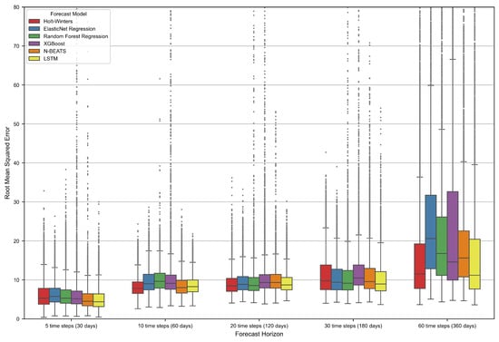
Figure 3. Box plots of RMSE values obtained for the evaluated forecasting models across different forecast horizons. Each box represents the distribution of RMSE values for a given model, including the median, quartile range (box), and variability (whiskers and outliers).

Similar to the summary mean statistics of model performance, the RMSE distribution plots in Figure 3 indicate that prediction uncertainty and the quantity of outliers are increasing with growing forecast horizon. In general, the LSTM model exhibits a similar median RMSE to the Holt–Winters model, indicating a competitive performance of the DL model to a traditional time series forecasting method. For forecast horizons of 5, 10, and 20 time steps, the LSTM model achieved the lowest dispersion of the RMSE values of all models, with lower number of outliers (indicating samples where models failed to forecast the time series effectively). In the case of longer forecast lengths, the LSTM model exhibits better (h = 30) or comparative (h = 60) performance, but the number of large errors is slightly higher. In general, the data-driven models were characterized by an increasing number of outliers for longer forecast horizons. This might be attributed to a higher likeliness of the forecasted sequence to have a different distribution than training data, causing the models to fail in extrapolating and predicting non-linear patterns in long-term subsidence dynamics.

Looking at the RMSE distributions for short-term predictions (five time steps), it can be observed that all ML and DL models achieved median performance lower than the statistical model. This indicates that ML and DL methods can effectively capture short-term time series characteristics of the considered displacement dataset. However, it should be noted that models utilizing decision trees (random forest, XGBoost) yield more predictions deviating significantly from the actual value of displacement. This can be attributed to the inability of tree-based models to extrapolate outside the range of the training data. Such cases will occur in the center of the subsidence trough, where displacements reach the highest absolute values, extending beyond the training time series. In these points, the accuracy of tree-based models is likely to diminish, which will be further confirmed later in this section. A similar characteristic is observed for longer forecast horizons.

Relationships between predicted displacement values and the corresponding residuals (defined as differences between actual and predicted values of displacement) were examined using residual plots (Figure 4 and Figure 5), providing a visual means of assessing potential heteroscedastic patterns and biases in the forecasting results.

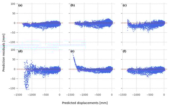
Figure 4. Residual plots of time series predictions, obtained from models trained to predict 5 time steps ahead. Based on predictions developed using models: (a) Holt–Winters exponential smoothing; (b) ElasticNet Regression; (c) random forest regression; (d) XGBoost; (e) N-BEATS; and (f) LSTM.

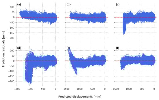
Figure 5. Residual plots of time series predictions, obtained from models trained to predict 30 time steps ahead. Based on predictions developed using models: (a) Holt–Winters exponential smoothing; (b) ElasticNet Regression; (c) random forest regression; (d) XGBoost; (e) N-BEATS; and (f) LSTM.

Residual plots for all six models, with forecast horizon of five steps, are presented in Figure 4. The Holt–Winters (Figure 4a), ElasticNet Regression (Figure 4b), and LSTM (Figure 4f) models show similar patterns of residual distribution. Residuals for these models show a homoscedastic pattern of distribution with a slight bias visible for higher subsidence prediction values. Prediction residuals between −400 and 0 mm exhibit symmetrical distribution around zero. Around −600 mm, a cluster of higher negative residuals occurs in the majority of models. This could likely be an indicator of a problem with accurate prediction of subsidence of this magnitude, possibly related to a displacement pattern unidentified by the model. In the higher-subsidence-magnitude sections (up to −1400 mm), the models achieve low residual variance, while at the same time a slight negative bias can be observed, indicating that the models tend to underestimate larger displacement values (predicted subsidence lower than observed). The random forest model (Figure 4c) shows higher residual dispersion than the previously mentioned models. The residual plot for the XGBoost method (Figure 4d) shows a heteroscedastic pattern, starting in the displacement range of −1000 mm, further confirming that the XGBoost model fails to predict large subsidence due to extrapolation problems. While the N-BEATS model (Figure 4e) shows a good residual distribution up until predictions of −1300 mm, a cluster of high residuals is evident for highest subsidence values, showing that this model tends to overestimate very high displacements.

Figure 5 shows residual plots obtained for long-term forecasting models (forecast horizon of 30 time steps). The Holt–Winters (Figure 5a) and linear regression (Figure 5b) models achieve the best residual dispersion of all models. Both models also show bias towards positive residuals with increasing displacement magnitude, indicating that when forecasting further ahead, these models tend to overestimate the subsidence values (predicted subsidence higher than observed). The random forest (Figure 5c) and XGBoost (Figure 5d) tree-based models show similar residual distribution, with higher dispersion than the exponential smoothing or linear regression, and clear increase of models’ uncertainty with higher values of displacement, indicating heteroscedasticity. Similarly, the N-BEATS model (Figure 5e) also exhibits a heteroscedastic pattern with lower accuracy for higher displacement predictions, a property observed for this model in short-term forecasting as well. The LSTM model (Figure 5f) shows good residual spread across the subsidence prediction range, with a cluster of higher negative residual values for high displacement predictions. This infers that displacements in the center of the subsidence trough (where subsidence is the highest) might be underestimated by the model. This will be further explored in the following subsection.

Figure 6 shows an example of predicted displacement fields obtained with the long-term (30 time steps) forecasting models (cumulative values of vertical displacements between 20 May 2016 and 26 October 2020). As indicated previously in Figure 5, the Holt–Winters (Figure 6a), ElasticNet (Figure 6b), and the LSTM (Figure 6f) models, characterized by the best residual dispersion, predict the displacement field closely reflecting the SBAS-derived displacement field in the study area (Figure 2). The RF (Figure 6c) and XGBoost (Figure 6d) models clearly underestimated the total displacement values, while the N-BEATS model (Figure 6e) overestimated the total displacements in the central part of the subsidence zone.

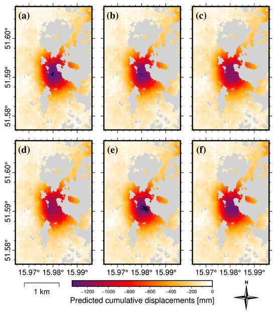
Figure 6. Maps of total displacements predicted with time series forecasting models for long-term horizon (30 time steps, 180 days). Based on predictions developed using models: (a) Holt–Winters exponential smoothing; (b) ElasticNet Regression; (c) random forest regression; (d) XGBoost; (e) N-BEATS; and (f) LSTM.

3.3. Displacement-Prediction-Error Analysis in the Spatial Domain

The analysis of summary statistics and distributions of accuracy metrics values, conducted in the previous subsection, revealed that machine learning models and neural networks perform similarly to statistical forecasting methods. However, a more detailed analysis of prediction residuals revealed certain characteristic patterns and biases, indicating the ineffectiveness of the evaluated models for a portion of the test dataset, specifically within certain displacement ranges. These characteristics can be observed mainly at high predicted subsidence values, as shown in the residual plots (Figure 4 and Figure 5), in the form of slight biases and heteroscedasticity of the forecast residuals.

Mining displacement time series can be highly heterogeneous, depending on location, exploitation parameters (e.g., seam thickness), and geological conditions. Therefore, in terms of operational application of ML and DL methods for forecasting mining displacement time series, forecast accuracy and outliers should be of the highest importance. The heterogeneous nature of subsidence time series should be accounted for, through analysis of spatial distributions of residuals and accuracy metrics. Clusters of residuals or higher-accuracy metrics may indicate that the predictive model does not consider certain characteristics and patterns in the training time series, or that new patterns, previously not present, have emerged. Subsidence forecasting for the protection of mining areas is expected to be uniformly effective across the entire subsidence trough. The central part of the trough undergoes the highest total subsidence, which may pose a challenge for models (lack of training data, inability to extrapolate beyond the training set). The edge areas of the subsiding zones, on the other hand, may be exposed to sudden non-linear changes, making effective prediction difficult.

An analysis of the spatial distribution of forecast errors was performed for test time series in the study area, considering differences in cumulative displacement values (displacement at the last time step) and RMSE distributions (corresponding to the ability to capture the dynamic progress of displacement over time). This assessed the models’ ability to predict total displacements over a specified time (residuals) and to model the dynamic progress of displacements over time, including possible non-linearities (RMSE).

Figure 7 shows the residual values for short-term (five time steps) forecasts of total displacements (defined as the difference between the actual and predicted values for the last time series step). The residual maps show the spatial distributions of total displacement prediction errors for the evaluated models. Spatial clusters of negative residuals are visible in the western part of the subsidence zone, indicating that the predicted values are locally underestimated (predicted subsidence being lower than actual). This may indicate patterns in the test data that were not taken into account by the models. In the case of the XGBoost model (Figure 7d), there is a visible accumulation of negative values throughout the central part of the basin, which confirms the inability of this model to extrapolate high subsidence. The N-BEATS model (Figure 7e) has relatively low residuals, except for a cluster of high residuals in the center. This implies that high subsidence values are overestimated, which was also apparent in the residual plot (Figure 4e).

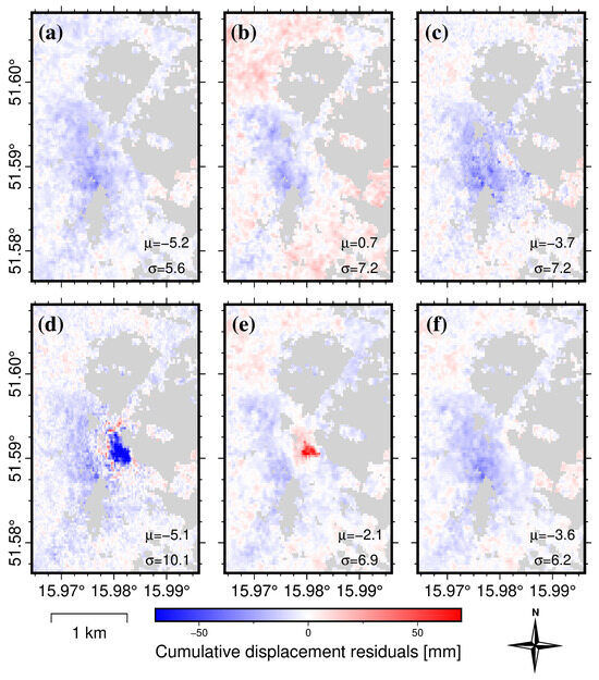
Figure 7. Residual maps of predicted cumulative displacements with forecast horizon = 5 steps (30 days), evaluating the model’s ability to forecast spatially heterogeneous time series. Based on predictions developed using models: (a) Holt–Winters exponential smoothing; (b) ElasticNet Regression; (c) random forest regression; (d) XGBoost; (e) N-BEATS; and (f) LSTM.

The spatial distribution of RMSE values calculated for models with a forecast horizon of five time steps is shown in Figure 8. Similarly to the total displacement residuals, clusters of higher error values are noticeable, particularly in the western and southwestern parts of the studied subsidence trough. The Holt–Winters (Figure 8a), ElasticNet (Figure 8b), and LSTM (Figure 8f) models demonstrate the most spatially uniform distribution of errors. Clusters of high values can be observed in the western part for the Holt–Winters method, as well as for the linear regression method, but with lower intensity. This may indicate potential locations with non-linear trends in the test series that were not found by the linear models. The N-BEATS (Figure 8e) and LSTM (Figure 8f) neural networks are characterized by the lowest error values in areas outside the subsidence trough, as well as the edges of the subsiding zone. These models also showed the lowest average RMSE values for the considered forecast horizon. However, it should be noted that clusters of large errors are present in the central part of the area for the N-BEATS model. The LSTM model shows a similar error distribution to the Holt–Winters model, which may indicate similar prediction problems for these models.

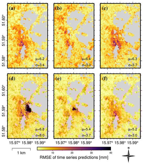
Figure 8. Maps of RMSE values for time series predictions in respective points. Based on predictions developed using models with forecast horizon of 5 time steps (multi-step short-term forecasting): (a) Holt–Winters exponential smoothing; (b) ElasticNet Regression; (c) random forest regression; (d) XGBoost; (e) N-BEATS; and (f) LSTM.

Figure 9 shows the forecast residuals for total displacement predictions with long-term forecasting models (30 time steps). Extending the forecast horizon increases the residual values. The lowest values and the most even spatial distribution are found again for the Holt–Winters (Figure 9a), ElasticNet (Figure 9b), and LSTM (Figure 9f) models. The tree-based models (Figure 9c,d) show clusters of high negative residuals for the highest subsidence values in the central part of the subsidence zone. The N-BEATS model underestimates subsidence in the entire area of the subsidence zone with the exception of the central part, where subsidence values were overestimated (Figure 9e). The Holt–Winters model (Figure 9a) regularly overestimates subsidence inside the studied area, which may indicate a change in the subsidence velocity that the trend forecasting model did not predict. The LSTM model (Figure 9f) and the ElasticNet model (Figure 9b) achieved better results in this aspect.

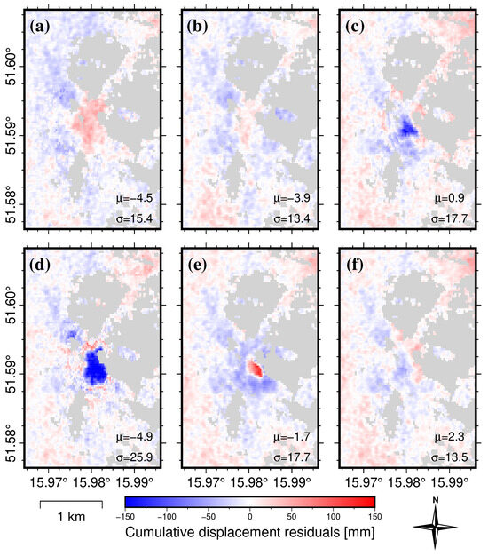
Figure 9. Residual maps of predicted cumulative displacements with forecast horizon = 30 steps (180 days), evaluating the models ability to forecast spatially heterogeneous time series. Based on predictions developed using models: (a) Holt–Winters exponential smoothing; (b) ElasticNet Regression; (c) random forest regression; (d) XGBoost; (e) N-BEATS; and (f) LSTM.

The assessment of the accuracy of time series modeling of displacements, performed using RMSE maps, is presented for long-term forecast models (h = 30) in Figure 10. Figure 10c–e indicate that tree-based and N-BEATS models, trained on heterogeneous time series data, are ineffective in forecasting high settlement values. The Holt–Winters model (Figure 10a) also exhibits error clustering, which may, again, indicate an incorrect estimation of the settlement trend by the model. The LSTM model (Figure 10f), despite obtaining valid forecasts for total displacements and the lowest mean RMSE, is characterized by numerous forecast outliers. This is mainly visible in the central part and in the northeast. The ElasticNet model (Figure 10b), on the other hand, is characterized by the absence of significant clusters of high errors within the center of the subsidence trough, which positions this model as the best for forecasting subsidence over a longer time horizon.

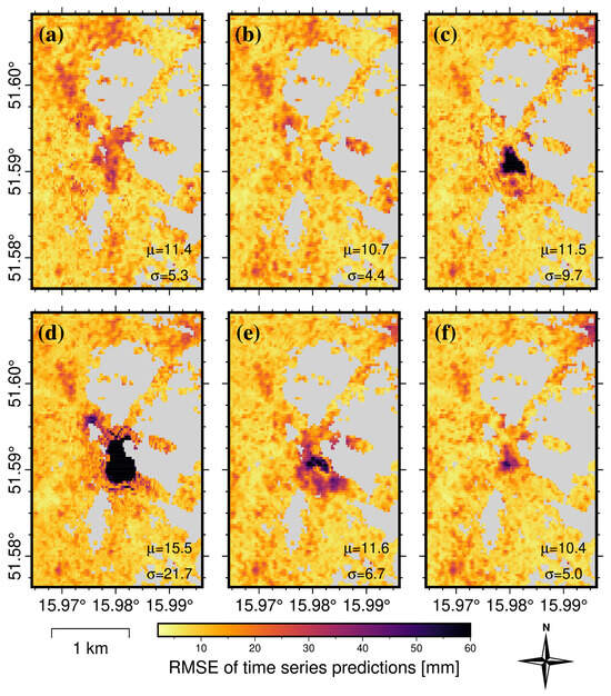
Figure 10. Maps of RMSE values calculated with time series predictions compared to actual InSAR displacements. Based on predictions developed using models with forecast horizon of 30 time steps (multi-step long-term forecasting): (a) Holt–Winters exponential smoothing; (b) ElasticNet Regression; (c) random forest regression; (d) XGBoost; (e) N-BEATS; and (f) LSTM.

4. Discussion

The findings of this study demonstrate and confirm that ML and DL methods can be used to develop models for predicting surface subsidence based on satellite InSAR measurements. Data-driven models, combined with an extensive time series dataset obtained through satellite measurements, can be an alternative to the approaches applied to these types of problems so far. Owing to their ability to model complex, non-linear relationships, machine learning methods can utilize the specific features and characteristics of time series in their predictions.

Building a model based on InSAR measurement results, especially in the case of univariate models, ties the accuracy of the model to the quality of the input data. In the case of InSAR methods, the accuracy of displacement measurements depends on a range of factors, including signal noise and coherence, atmospheric delays, and phase unwrapping errors. In order to ensure high quality of the predictive model, InSAR measurements should comprehensively incorporate corrections of potential errors. Additionally, being a remote sensing measurement method, its results should be verified using field measurement data whenever possible (e.g., leveling data) [59].

This study utilized SBAS measurements to both maximize the coverage of the study area and identify displacements outside built-up areas. Should the analysis focus on specific objects sensitive from the perspective of mining area protection, the methodology could also be based on measurements provided by other methods, such as PSInSAR or GNSS. The methodology could also consider integrating InSAR and GNSS methods, at the same time providing independent verification of InSAR measurements.

Development of models with different forecast horizons, including short- and long-term forecasts (from 1 month to 1 year), allowed examination of forecast accuracy related to the length of the forecast horizon. According to the obtained results, the models’ accuracy depends on the length of the forecast horizon, with longer horizons resulting in increasing model errors. This problem is particularly noticeable in areas with non-linear subsidence trends, where specific time series patterns may not be recognized by the model. The conducted study also showed that in an operational environment, an optimal forecast horizon should consider both practical requirements and model accuracy.

The InSAR measurement data used in the article cover vertical ground displacements in an area of active underground mining. These displacements have a form of subsidence, primarily characterized by a variable trend with limited seasonal patterns. With such data, autoregressive and linear models can achieve a similar performance to more complex deep neural network models. It is also worth noting that the study did not take into account displacements characterized by rapid changes in velocity in this study area, which are caused by seismic tremors induced by mining activity. In order to create a predictive model that considers such characteristics in the time series, it would be necessary to expand the univariate model formula and implement a multivariate model with additional variables explaining the rapid velocity changes. These could include geological data, as well as seismic event catalogs. Accounting for dynamic events influencing the subsidence process could enable the development of a more complex model with better generalization capabilities [60]. A potential approach to explore in a future study would be to expand the time series forecasting model with dynamic covariates describing the seismic events, or to apply an anomaly detection model that could implement updates to the model’s predictions (e.g., through short-term forecast of tremor-induced subsidence).

Machine learning models and neural networks in this paper were established as global models, trained on time series sampled from the entire study area. When investigating a subsidence trough, the time series across its area are heterogeneous, with local clusters of stable points and points with varying magnitudes of subsidence, as well as points with variable time series patterns, where the subsidence has just begun or has already ended. Using global models in the methodology makes it feasible to forecast time series with different characteristics. The model is more scalable and efficient than local models trained on individual time series. The global model, which uses patterns recognized in the time series data, can be used for forecasting in mining areas with similar mining and geological conditions. In areas undergoing deformations of various types (e.g., within different subsidence troughs), an alternative solution would be to create local models for individual subsidence zones. The applicability of such local models in other subsidence zones (e.g., through a transfer learning approach) could be the subject of further research.

The limitations of the proposed methodology are primarily related to the nature of the input data. Univariate models based solely on InSAR data do not consider complex geomechanical mechanisms that influence the subsidence behavior. Therefore, the prediction accuracy depends on the InSAR measurement accuracy; hence, research on this topic should also integrate verification with other independent measurement method, if available. Moreover, expanding the univariate approach (utilizing only displacement history) into a multivariate solution would allow the model to capture the physical drivers of subsidence. This would require integrating specific geospatial data sources into the forecasting model, including e.g., locations of mine panels and panel extraction data (considering the temporal evolution of production), published seismic event catalogs (particularly for seismic tremors influencing the subsidence behavior), and geological maps with fault locations and lithology.

Despite the identified limitations, the results of the study confirm the potential of applying machine learning methods to deformation forecasting in mining areas. This study demonstrated the effectiveness of an LSTM-based DL architecture in predicting InSAR-derived subsidence. Combining satellite monitoring methods, acquiring extensive measurement datasets, with data-driven models allows for effective monitoring and prediction of deformation with high temporal and spatial resolution. A potential implementation of this approach into a monitoring and early warning system would enable pseudo-continuous subsidence monitoring at crucial locations. At the same time, the system could forecast subsidence values and detect anomalies in the subsidence pattern. As subsequent satellite imagery becomes available (e.g., every 6 days with the Sentinel-1 mission), both the measured values and the predictive model would be updated.

While mean accuracy metrics provide insight into the overall performance of time series forecasting models, they may obscure important spatial variability of forecast errors and prediction quality, as indicated in this article. For ground deformation monitoring context, local behavior of displacements is of critical importance for effective predictive modeling, possibly indicating subsidence accelerations and anomalous behavior. Spatial assessment of models’ accuracy can provide a more comprehensive understanding of model generalization capabilities. This can be particularly relevant when applying data-driven forecasting models in heterogeneous mining areas, where deformation dynamics can vary over short distances. Incorporating spatial analysis of forecast errors into the model validation process can, therefore, support the development of more reliable and interpretable forecasting systems for ground deformation monitoring.

5. Conclusions

This study assessed the performance of ML and DL models in forecasting InSAR-derived displacement time series in a mining subsidence scenario. Data-driven models were evaluated in terms of performance relative to the length of forecast horizon, considering both short-term (1-month ahead) and long-term (1-year ahead) time series forecasts.

The results demonstrated that ensemble tree-based methods (random forest, XGBoost) achieved the lowest prediction accuracy according to the RMSE, MAE, and sMAPE measures, due to the nature of the processed input data and inability to extrapolate higher subsidence values. The linear regression model performed comparatively to the baseline exponential smoothing approach, while DL-based approaches (N-BEATS, LSTM) often achieved a comparative or superior performance, albeit with numerous outliers. Based on the prediction results, it was shown that while more complex models can achieve satisfactory results, a careful examination benchmarking various data-driven models is recommended for the optimal model selection in practical scenarios.

A detailed forecast error analysis in both spatial and temporal domains indicated certain problems with ML and DL models’ performance, emphasizing that the models are underperforming most often in predicting displacements in the central part of the subsidence trough, where absolute vertical displacement values are the highest. The results also indicated that forecast errors tend to concentrate in specific locations, suggesting that certain time series patterns typical to these locations would not be captured by the models.

This study contributes to the development of predictive deformation monitoring frameworks, based on open satellite-derived data and open-source software. Based on the presented results, it can be concluded that a thorough analysis of forecast accuracy metrics and forecast errors, considering both temporal and spatial domains, is essential when dealing with a data-driven model for displacement prediction.

Future works will include the incorporation of other mining and geological variables into time series forecasting models, the application of a suite of models attributed locally to different subsidence zones (with transfer learning capability evaluation), and the testing of other neural network models (including attention-based architectures) for time series forecasting with improved explainability.

References

- Kratzsch, H. Mining Subsidence Engineering; Springer: Berlin/Heidelberg, Germany, 1983. [Google Scholar] [CrossRef]
- Tondaś, D.; Kazmierski, K.; Kapłon, J. Real-Time and Near Real-Time Displacement Monitoring With GNSS Observations in the Mining Activity Areas. IEEE J. Sel. Top. Appl. Earth Obs. Remote Sens. 2023, 16, 5963–5972. [Google Scholar] [CrossRef]
- Tajduś, K.; Sroka, A.; Misa, R.; Hager, S.; Rusek, J.; Dudek, M.; Wollnik, F. Analysis of Mining-Induced Delayed Surface Subsidence. Minerals 2021, 11, 1187. [Google Scholar] [CrossRef]
- Witkowski, W.T.; Łukosz, M.; Guzy, A.; Hejmanowski, R. Estimation of Mining-Induced Horizontal Strain Tensor of Land Surface Applying InSAR. Minerals 2021, 11, 788. [Google Scholar] [CrossRef]
- Ćwiąkała, P.; Gruszczyński, W.; Stoch, T.; Puniach, E.; Mrocheń, D.; Matwij, W.; Matwij, K.; Nędzka, M.; Sopata, P.; Wójcik, A. UAV Applications for Determination of Land Deformations Caused by Underground Mining. Remote Sens. 2020, 12, 1733. [Google Scholar] [CrossRef]
- Witkowski, W.T.; Mrocheń, D.; Sopata, P.; Stoch, T. Integration of the Leveling Observations and PSInSAR Results for Monitoring Deformations Caused by Underground Mining. In Proceedings of the 2021 IEEE International Geoscience and Remote Sensing Symposium IGARSS, Brussels, Belgium, 11–16 July 2021; pp. 6614–6617. [Google Scholar] [CrossRef]
- Knothe, S. Równanie Profilu Ostatecznie Wykształconej Niecki Osiadania. Archiwum Górnictwa i Hutnictwa 1953, 1, 22–38. [Google Scholar]
- Luo, Y. An Improved Influence Function Method for Predicting Subsidence Caused by Longwall Mining Operations in Inclined Coal Seams. Int. J. Coal Sci. Technol. 2015, 2, 163–169. [Google Scholar] [CrossRef]
- Apanowicz, B.; Milczarek, W.; Kowalski, A. Novel Method for Determining the Time Coefficient c in Knothe’s Function and Disappearance Time of Deformation Increase Using SAR Data. Measurement 2024, 235, 114898. [Google Scholar] [CrossRef]
- Chen, Y.; Zha, J.; Wang, L. Adaptive Dynamic Prediction Model of Mining Subsidence Aided by Measured Data. Sci. Rep. 2025, 15, 14754. [Google Scholar] [CrossRef]
- Knothe, S.M. Prognozowanie Wpływów Eksploatacji Górniczej; Wydaw. Śląsk: Katowice, Poland, 1984. [Google Scholar]
- Kochmański, T. Całkowa Teoria Ruchów Górotworu Nad Eksploatacją Złoża Pokładowego Na Podstawie Pomiarów Geodezyjnych. Geod. Kartogr. 1955, 2. [Google Scholar]
- Litwiniszyn, J. Przemieszczenia Górotworu w Świetle Teorii Prawdopodobieństwa. Arch. Górnictwa Hut. 1954, 1. [Google Scholar]
- Drzęźla, B. Przybliżona Ocena Niektórych Parametrów Kinematyki Niecki Osiadania Przy Zmianach Prędkości Wybierania i Postojach Ścian. Przegląd Górniczy 1995, 9, 10–16. [Google Scholar]
- Dudek, M.; Mrocheń, D.; Sroka, A.; Tajduś, K. Integrating the Finite Element Method with Python Scripting to Assess Mining Impacts on Surface Deformations. Appl. Sci. 2024, 14, 7797. [Google Scholar] [CrossRef]
- Li, P.; Tan, Z.; Yan, L.; Deng, K. Time Series Prediction of Mining Subsidence Based on a SVM. Min. Sci. Technol. 2011, 21, 557–562. [Google Scholar] [CrossRef]
- Rahmati, O.; Falah, F.; Naghibi, S.A.; Biggs, T.; Soltani, M.; Deo, R.C.; Cerdà, A.; Mohammadi, F.; Tien Bui, D. Land Subsidence Modelling Using Tree-Based Machine Learning Algorithms. Sci. Total Environ. 2019, 672, 239–252. [Google Scholar] [CrossRef] [PubMed]
- Yang, W.; Xia, X. Prediction of Mining Subsidence under Thin Bedrocks and Thick Unconsoliyeard Layers Based on Field Measurement and Artificial Neural Networks. Comput. Geosci. 2013, 52, 199–203. [Google Scholar] [CrossRef]
- Cieślik, K.; Milczarek, W. Application of Machine Learning in Forecasting the Impact of Mining Deformation: A Case Study of Underground Copper Mines in Poland. Remote Sens. 2022, 14, 4755. [Google Scholar] [CrossRef]
- Hill, P.; Biggs, J.; Ponce-López, V.; Bull, D. Time-Series Prediction Approaches to Forecasting Deformation in Sentinel-1 InSAR Data. J. Geophys. Res. Solid Earth 2021, 126, e2020JB020176. [Google Scholar] [CrossRef]
- Chen, B.; Yu, H.; Zhang, X.; Li, Z.; Kang, J.; Yu, Y.; Yang, J.; Qin, L. Time-Varying Surface Deformation Retrieval and Prediction in Closed Mines through Integration of SBAS InSAR Measurements and LSTM Algorithm. Remote Sens. 2022, 14, 788. [Google Scholar] [CrossRef]
- Moualla, L.; Rucci, A.; Naletto, G.; Anantrasirichai, N.; Da Deppo, V. Hybrid GIS-Transformer Approach for Forecasting Sentinel-1 Displacement Time Series. Remote Sens. 2025, 17, 2382. [Google Scholar] [CrossRef]
- Wang, J.; Fan, X.; Zhang, Z.; Zhang, X.; Nie, W.; Qi, Y.; Zhang, N. Spatiotemporal Mechanism-Based Spacetimeformer Network for InSAR Deformation Prediction and Identification of Retrogressive Thaw Slumps in the Chumar River Basin. Remote Sens. 2024, 16, 1891. [Google Scholar] [CrossRef]
- Zhou, C.; Ye, M.; Xia, Z.; Wang, W.; Luo, C.; Muller, J.P. An Interpretable Attention-Based Deep Learning Method for Landslide Prediction Based on Multi-Temporal InSAR Time Series: A Case Study of Xinpu Landslide in the TGRA. Remote Sens. Environ. 2025, 318, 114580. [Google Scholar] [CrossRef]
- Cao, Y.; Zhou, X.; Yan, K. Deep Learning Neural Network Model for Tunnel Ground Surface Settlement Prediction Based on Sensor Data. Math. Probl. Eng. 2021, 2021, 9488892. [Google Scholar] [CrossRef]
- Wright, P.; Stow, R. Detecting Mining Subsidence from Space. Int. J. Remote Sens. 1999, 20, 1183–1188. [Google Scholar] [CrossRef]
- Raspini, F.; Caleca, F.; Del Soldato, M.; Festa, D.; Confuorto, P.; Bianchini, S. Review of Satellite Radar Interferometry for Subsidence Analysis. Earth-Sci. Rev. 2022, 235, 104239. [Google Scholar] [CrossRef]
- Ferretti, A.; Prati, C.; Rocca, F. Permanent Scatterers in SAR Interferometry. IEEE Trans. Geosci. Remote Sens. 2001, 39, 8–20. [Google Scholar] [CrossRef]
- Antonielli, B.; Sciortino, A.; Scancella, S.; Bozzano, F.; Mazzanti, P. Tracking Deformation Processes at the Legnica Glogow Copper District (Poland) by Satellite InSAR—I: Room and Pillar Mine District. Land 2021, 10, 653. [Google Scholar] [CrossRef]
- Berardino, P.; Fornaro, G.; Lanari, R.; Sansosti, E. A New Algorithm for Surface Deformation Monitoring Based on Small Baseline Differential SAR Interferograms. IEEE Trans. Geosci. Remote Sens. 2002, 40, 2375–2383. [Google Scholar] [CrossRef]
- Gee, D.; Bateson, L.; Sowter, A.; Grebby, S.; Novellino, A.; Cigna, F.; Marsh, S.; Banton, C.; Wyatt, L. Ground Motion in Areas of Abandoned Mining: Application of the Intermittent SBAS (ISBAS) to the Northumberland and Durham Coalfield, UK. Geosciences 2017, 7, 85. [Google Scholar] [CrossRef]
- Samsonov, S.; d’Oreye, N.; Smets, B. Ground Deformation Associated with Post-Mining Activity at the French–German Border Revealed by Novel InSAR Time Series Method. Int. J. Appl. Earth Obs. Geoinf. 2013, 23, 142–154. [Google Scholar] [CrossRef]
- Hochreiter, S.; Schmidhuber, J. Long Short-Term Memory. Neural Comput. 1997, 9, 1735–1780. [Google Scholar] [CrossRef]
- Piestrzyński, A. Monografia KGHM Polska Miedź SA, 2nd ed.; KGHM CUPRUM Sp. z o.o. CBR: Wrocław, Poland, 2008. [Google Scholar]
- Butra, J.; Kicki, J. Ewolucja Technologii Eksploatacji Złóż Rud Miedzi w Polskich Kopalniach; Biblioteka Szkoły Eksploatacji Podziemnej: Kraków, Poland, 2003. [Google Scholar]
- Kudłacik, I.; Kapłon, J.; Lizurek, G.; Crespi, M.; Kurpiński, G. High-Rate GPS Positioning for Tracing Anthropogenic Seismic Activity: The 29 January 2019 Mining Tremor in Legnica- Głogów Copper District, Poland. Measurement 2021, 168, 108396. [Google Scholar] [CrossRef]
- Milczarek, W. Application of a Small Baseline Subset Time Series Method with Atmospheric Correction in Monitoring Results of Mining Activity on Ground Surface and in Detecting Induced Seismic Events. Remote Sens. 2019, 11, 1008. [Google Scholar] [CrossRef]
- Hejmanowski, R.; Malinowska, A.A.; Witkowski, W.T.; Guzy, A. An Analysis Applying InSAR of Subsidence Caused by Nearby Mining-Induced Earthquakes. Geosciences 2019, 9, 490. [Google Scholar] [CrossRef]
- Rosen, P.A.; Gurrola, E.; Sacco, G.F.; Zebker, H. The InSAR Scientific Computing Environment. In Proceedings of the EUSAR 2012, 9th European Conference on Synthetic Aperture Radar, Nuremberg, Germany, 23–26 April 2012; pp. 730–733. [Google Scholar]
- Farr, T.G.; Rosen, P.A.; Caro, E.; Crippen, R.; Duren, R.; Hensley, S.; Kobrick, M.; Paller, M.; Rodriguez, E.; Roth, L.; et al. The Shuttle Radar Topography Mission. Rev. Geophys. 2007, 45, 1–33. [Google Scholar] [CrossRef]
- Goldstein, R.M.; Werner, C.L. Radar Interferogram Filtering for Geophysical Applications. Geophys. Res. Lett. 1998, 25, 4035–4038. [Google Scholar] [CrossRef]
- Chen, C.W.; Zebker, H.A. Network Approaches to Two-Dimensional Phase Unwrapping: Intractability and Two New Algorithms. J. Opt. Soc. Am. A 2000, 17, 401–414. [Google Scholar] [CrossRef]
- Yunjun, Z.; Fattahi, H.; Amelung, F. Small Baseline InSAR Time Series Analysis: Unwrapping Error Correction and Noise Reduction. Comput. Geosci. 2019, 133, 104331. [Google Scholar] [CrossRef]
- Yu, C.; Li, Z.; Penna, N.T.; Crippa, P. Generic Atmospheric Correction Model for Interferometric Synthetic Aperture Radar Observations. J. Geophys. Res. Solid Earth 2018, 123, 9202–9222. [Google Scholar] [CrossRef]
- Wright, T.J.; Parsons, B.E.; Lu, Z. Toward Mapping Surface Deformation in Three Dimensions Using InSAR. Geophys. Res. Lett. 2004, 31, L01607. [Google Scholar] [CrossRef]
- Samieie-Esfahany, S.; Hanssen, R.F.; Van Thienen-Visser, K.; Muntendam-Bos, A. On the Effect of Horizontal Deformation on Insar Subsidence Estimates. In Proceedings of the Fringe 2009 Workshop, Frascati, Italy, 30 November–4 December 2009; pp. 1–7. [Google Scholar]
- Costantini, M.; Minati, F.; Trillo, F.; Ferretti, A.; Novali, F.; Passera, E.; Dehls, J.; Larsen, Y.; Marinkovic, P.; Eineder, M.; et al. European Ground Motion Service (EGMS). In Proceedings of the 2021 IEEE International Geoscience and Remote Sensing Symposium IGARSS, Brussels, Belgium, 11–16 July 2021; pp. 3293–3296. [Google Scholar] [CrossRef]
- Hyndman, R.J.; Athanasopoulos, G. Forecasting: Principles and Practice, 3rd ed.; OTexts: Melbourne, Australia, 2021. [Google Scholar]
- Garza, A.; Canseco, M.M.; Challú, C.; Olivares, K.G. StatsForecast: Lightning Fast Forecasting with Statistical and Econometric Models; PyCon: Salt Lake City, UT, USA, 2022. [Google Scholar]
- Zou, H.; Hastie, T. Regularization and Variable Selection Via the Elastic Net. J. R. Stat. Soc. Ser. B Stat. Methodol. 2005, 67, 301–320. [Google Scholar] [CrossRef]
- Breiman, L. Random Forests. Mach. Learn. 2001, 45, 5–32. [Google Scholar] [CrossRef]
- Chen, T.; Guestrin, C. XGBoost: A Scalable Tree Boosting System. In Proceedings of the 22nd ACM SIGKDD International Conference on Knowledge Discovery and Data Mining, San Francisco, CA, USA, 13–17 August 2016; Association for Computing Machinery: New York, NY, USA, 2016; KDD’16, pp. 785–794. [Google Scholar] [CrossRef]
- Oreshkin, B.N.; Carpov, D.; Chapados, N.; Bengio, Y. N-BEATS: Neural Basis Expansion Analysis for Interpretable Time Series Forecasting. arXiv 2019, arXiv:1905.10437. [Google Scholar] [CrossRef]
- Witkowski, W.T.; Łucka, M.; Guzy, A.; Sudhaus, H.; Barańska, A.; Hejmanowski, R. Impact of Mining-Induced Seismicity on Land Subsidence Occurrence. Remote Sens. Environ. 2024, 301, 113934. [Google Scholar] [CrossRef]
- Milczarek, W.; Kopeć, A.; Głąbicki, D.; Bugajska, N. Induced Seismic Events—Distribution of Ground Surface Displacements Based on InSAR Methods and Mogi and Yang Models. Remote Sens. 2021, 13, 1451. [Google Scholar] [CrossRef]
- Owczarz, K.; Blachowski, J. Random Forest—Based Identification of Factors Influencing Ground Deformation Due to Mining Seismicity. Remote Sens. 2024, 16, 2742. [Google Scholar] [CrossRef]
- Maghsoudi, Y.; Hooper, A.J.; Wright, T.J.; Lazecky, M.; Ansari, H. Characterizing and Correcting Phase Biases in Short-Term, Multilooked Interferograms. Remote Sens. Environ. 2022, 275, 113022. [Google Scholar] [CrossRef]
- Karami, E.; Shami, S.; Maghsoudi, Y.; Ranjgar, B.; Azadnejad, S. Investigating the InSAR Phase Bias in the SBAS Algorithm and Its Effect on Different Landcovers. IEEE Access 2025, 13, 82514–82526. [Google Scholar] [CrossRef]
- Tao, Q.; Xiao, Y.; Hu, L.; Liu, R.; Li, X. Ground Subsidence Prediction with High Precision: A Novel Spatiotemporal Prediction Model with Interferometric Synthetic Aperture Radar Technology. Int. J. Remote Sens. 2024, 45, 8649–8671. [Google Scholar] [CrossRef]
- Zhang, J.; Gao, J.; Gao, F. Time Series Land Subsidence Monitoring and Prediction Based on SBAS-InSAR and GeoTemporal Transformer Model. Earth Sci. Inform. 2024, 17, 5899–5911. [Google Scholar] [CrossRef]
Disclaimer/Publisher’s Note: The statements, opinions and data contained in all publications are solely those of the individual author(s) and contributor(s) and not of MDPI and/or the editor(s). MDPI and/or the editor(s) disclaim responsibility for any injury to people or property resulting from any ideas, methods, instructions or products referred to in the content. |
© 2025 by the author. Licensee MDPI, Basel, Switzerland. This article is an open access article distributed under the terms and conditions of the Creative Commons Attribution (CC BY) license (https://creativecommons.org/licenses/by/4.0/).