A Semi-Analytical–Empirical Hybrid Model for Shallow Water Bathymetry Using Multispectral Imagery Without In Situ Data

Highlights

What are the main findings?

• A novel semi-analytical–empirical hybrid model was developed to retrieve shallow-water bathymetry from multispectral imagery containing only three visible bands, without relying on in situ depth measurements.
• The proposed model outperformed traditional physics-based methods across four coral reef environments, achieving root-mean-square error (RMSE) values ranging from 0.98 to 1.62 m, mean absolute error (MAE) values between 0.73 and 1.13 m, and coefficients of determination (R²) from 0.91 to 0.95.

What are the implications of the main findings?

• The model enables reliable and highly accurate bathymetric mapping in regions lacking field measurements, providing a robust alternative to existing physics-based approaches.
• The findings offer practical guidance for bathymetric retrieval using band-limited satellite imagery and contribute to advancing optical remote sensing of underwater topography.

Abstract

Water depth in shallow marine environments is a fundamental parameter for oceanographic research and coastal engineering applications. High-resolution satellite imagery and long-term medium-resolution imagery offer significant potential for detailed bathymetric mapping and monitoring spatiotemporal variations in bathymetry. However, most of these images contain only three visible bands (blue, green, and red), making bathymetric mapping from such images challenging in practical applications. For the empirical approach, high-quality in situ depth calibration data, which are essential for establishing a reliable empirical bathymetric model, are either unavailable or excessively expensive. For the physics-based approach, images containing only three visible bands can be problematic in accurately deriving depths. To address this limitation, this study proposes a novel semi-analytical-empirical hybrid model for water depth retrieval. The core of the proposed method is the integration of a semi-analytical model with a physics-based dual-band model. This integration quantifies the relative depth relationships among pixels and uses them as a physical constraint. Through this constraint, the method identifies physically reliable depth estimates from the multiple numerical solutions of the semi-analytical model for a subset of shallow-water pixels, which then serve as an in situ–free calibration dataset. This dataset is subsequently used to determine the empirically based optimal retrieval model, which is finally applied to generate the complete bathymetric map. The results from four typical coral reef regions—Buck Island, Yongxing Island, Kaneohe Bay, and Yongle Atoll—demonstrated that the proposed model achieved root-mean-square errors (RMSE) of 0.98–1.62 m, mean absolute errors (MAE) of 0.73–1.13 m, and coefficients of determination (R²) of 0.91–0.95 in comparison to in situ measurements. Compared to both the physics-based dual-band model and the L-S model (i.e., the bathymetry mapping approach combining Log-ratio and Semi-analytical models), the proposed model reduced the RMSE by 9–55%, reduced the MAE by 4–56%, and improved the R² by 0.01–0.29. Additionally, the accuracy of the proposed model surpasses that of both the physics-based dual-band model and the L-S model across all depth intervals, particularly in deeper depth waters (>15 m). This study offers a robust solution for bathymetric mapping in areas lacking in situ depth data and contributes significantly to advancing optical remote sensing techniques for underwater topography detection.

1. Introduction

Shallow water depth is a critical parameter in the marine environment, playing a significant role in navigation safety, marine resource exploitation, and environmental monitoring [1,2,3]. Traditional bathymetric techniques, such as shipborne single- and multi-beam sonar and airborne LiDAR bathymetry systems, provide high measurement accuracy but are costly and difficult to deploy over large areas [4,5,6]. In contrast, satellite-based techniques for bathymetry retrieval are cost-effective, offer extensive coverage, and provide timely data, making them an essential complement to traditional bathymetric surveys [7,8,9].

Optical satellite-based bathymetry approaches are broadly classified into empirical and physics-based approaches [10,11]. Empirical approaches establish statistical relationships between spectral indices and water depth for bathymetry mapping [12,13]. Due to their simplicity and operational convenience, these approaches are widely used. Common models in this category include the band logarithmic ratio model, the multi-band model, and machine learning models [14,15,16,17,18]. Despite their maturity, empirical approaches heavily depend on in situ depth data and demonstrate limited generalizability, typically performing well only in localized areas represented by the calibration data. Although some studies have explored using ICESat-2 satellite bathymetry data as an alternative calibration source, the spatial coverage of its ground tracks remains incomplete, potentially lacking data support for certain small atolls and coastal zones [19,20,21].

In contrast, physics-based approaches do not rely on in situ depth measurements; instead, they estimate water depth using bio-optical radiative transfer theory [22]. These approaches can be categorized into semi-analytical models, semi-analytical-empirical hybrid models, and adaptive bathymetry estimation models [23]. The Hyperspectral Optimization Process Exemplar (HOPE) model, developed by Lee et al., is a representative semi-analytical bathymetry model that simultaneously retrieves water depth, bottom reflectance, and water optical properties through nonlinear optimization [24,25,26]. Since semi-analytical models involve at least five unknown parameters, hyperspectral data—characterized by numerous narrow and contiguous spectral bands—are more suitable for their application than multispectral data. Nevertheless, semi-analytical models can also be applied to certain satellite multispectral imagery (e.g., Landsat-8/9 and WorldView-2/3), which typically include at least four visible bands (coastal, blue, green, and red) [27,28,29,30]. However, the number of visible bands varies across different satellite-based optical images, significantly affecting the retrieval accuracy of semi-analytical models applied to multispectral imagery. The use of semi-analytical models is limited for most high-spatial-resolution images (e.g., IKONOS-2, QuickBird-2, GeoEye-1, SPOT-6/7, DOVE-C, Ziyuan-3, Gaofen-1/2/7, RapidEye, SuperView-1) and some historical 30 m medium-spatial-resolution images (e.g., Landsat-5/7) because these sensors provide only three visible bands (blue, green, and red) suitable for bathymetry retrieval.

High-resolution imagery holds significant potential for mapping detailed bathymetry, while Landsat-5/7 imagery, spanning two decades, provides valuable data for monitoring spatiotemporal changes in underwater topography. In regions lacking in situ depth measurements, there is a clear need to leverage the strengths of these multispectral data sources. Consequently, developing a physics-based bathymetry model tailored for multispectral imagery with only three visible bands is highly desirable, as such a model eliminates reliance on costly and labor-intensive in situ depth measurements, enabling high-resolution bathymetric mapping and long-term monitoring of bathymetric changes in areas with scarce field data. To this end, semi-analytical-empirical hybrid models, as well as adaptive bathymetry estimation models, have been proposed [31,32,33]. Semi-analytical-empirical hybrid models assume a relative relationship among the water depths of different pixels, enabling the extraction of physically valid depths for a subset of shallow-water pixels using a semi-analytical model. These valid depths are then used to calibrate an empirical approach for bathymetric mapping of the entire area [34]. A typical example is the L-S model, which combines a semi-analytical model with the band logarithmic ratio model developed by Xia et al. [32]. However, the L-S model may produce significant retrieval errors due to potential spurious correlations between the semi-analytically estimated depths and the band logarithmic ratios. Adaptive bathymetry estimation models first derive the analytical expression of an empirical approach, then solve for all unknown parameters using pixels sampled from the image to achieve bathymetry retrieval [35,36]. Notable examples include the adaptive band logarithmic ratio model by Li et al. and the physics-based dual-band model by Chen et al. [31,33]. Nevertheless, both models are sensitive to non-ideal sampled pixels of deep-water regions, and the physics-based dual-band model is challenging to apply in waters lacking a defined waterline. In summary, semi-analytical models are unsuitable for mapping bathymetry from multispectral imagery with only three visible bands. Although existing semi-analytical-empirical hybrid models and adaptive bathymetry estimation models can retrieve depths from such imagery, the reliability of their results remains inadequate.

This study aims to address the limitations of existing bathymetry retrieval methods, which often struggle to generate robust and accurate bathymetric maps using multispectral imagery containing only three visible bands in areas lacking field depth data. To this end, we propose a novel semi-analytical-empirical hybrid model for shallow bathymetry retrieval using such band-limited imagery, eliminating the need for in situ depth data. The core of our method lies in integrating the semi-analytical model with the analytical expression of the physics-based dual-band model. This integration is designed to quantify the relative depth relationships among pixels, which then serve as a physical constraint to identify valid water depths from the multiple numerical solutions of the semi-analytical model for shallow-water pixels. By resolving this solution ambiguity, we obtain a set of physically reliable depths for a subset of shallow-water pixels. These retrieved depths subsequently form an in situ–free calibration dataset, which is used to determine the empirically based optimal retrieval model (from the optimal combination of depth factors and empirical models) for generating the complete bathymetric map. The effectiveness of the proposed model is validated using Gaofen-2 imagery of Kaneohe Bay and Sentinel-2 images of Buck Island, Yongle Atoll, and Yongxing Island. Its retrieval accuracy is rigorously evaluated and compared with that of baseline methods, such as the physics-based dual-band model and the L-S model.

2. Study Area and Data

2.1. Study Area

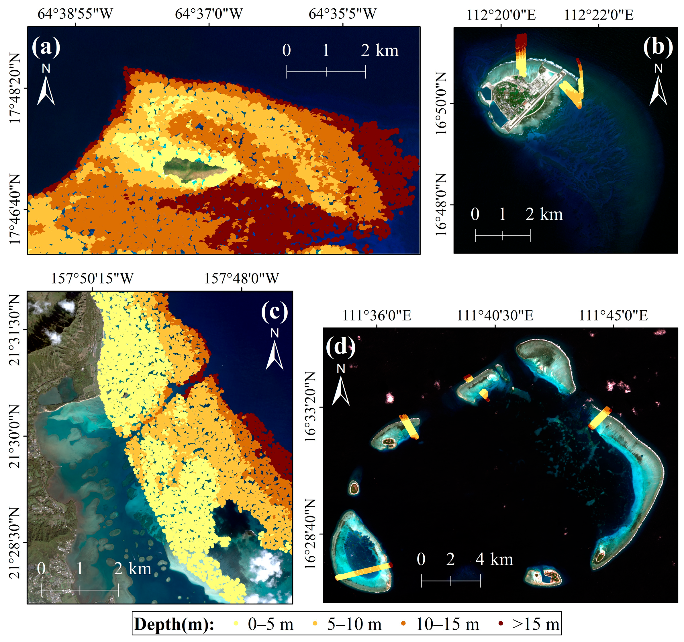
In this study, four representative coral reef environments—Buck Island, Yongxing Island, Kaneohe Bay, and Yongle Atoll—were selected as the study areas (Figure 1).

Buck Island, centered at approximately 17°47′N, 64°37′W, lies about 2.4 km northeast of St. Croix in the U.S. Virgin Islands. An emergent reef bank surrounds Buck Island, creating a lagoon that is 50–150 m wide and 2–4 m deep. This lagoon begins on the southern side and extends counterclockwise to the northwest corner, where it ends and becomes a series of isolated patch reefs. The surrounding waters are highly transparent, characteristic of Case-I tropical waters, and the benthic substrates primarily consist of coral reefs, sand, and seagrass.

Yongxing Island, centered at approximately 16°50′N, 112°20′E, is the largest island in the Xisha Islands. It is a coral island covering an area of about 3.08 km² and has an irregular oval shape. The island features sandy beaches and supports sparse coastal vegetation. The nearshore zone consists of shallow reef flats and sandy substrates, surrounded by clear Case-I waters. Chlorophyll a concentrations in the waters range from 0.02 to 0.4 µg/L, and water transparency can reach up to 30 m.

Kaneohe Bay, centered at approximately 21°29′N, 157°49′W, lies on the northeastern coast of Oahu Island, HI, USA. It is a partially enclosed embayment with an average depth of 8 m and features a sizeable lagoon area. Fringing reefs are widely distributed along its coastlines, and numerous reefs are found within the lagoon. Outside the lagoon, there is a crescent-shaped reef approximately 5 km long and 2 km wide, featuring a steep reef slope on the seaward side. Kaneohe Bay also has a prominent tidal channel that connects the coral reef bay to the open ocean, allowing large volumes of seawater to flow in and out with the rising and falling tides. The bay exhibits significant spatial heterogeneity in the optical properties of its waters. The waters in the northwest and offshore regions of Kaneohe Bay display high transparency, resembling the characteristics of the surrounding Case-I water bodies. In contrast, the nearshore areas, particularly the southeastern waters with increased enclosure, exhibit significantly lower transparency.

Yongle Atoll, centered at approximately 16°30′N, 111°41′E, is located in the western Xisha Islands of the South China Sea. It is a large, discontinuous open atoll primarily composed of seven named coral reef flats—Quanfu Island, Shanhu Island, Ganquan Island, Antelope Reef, Chenhang Island, Jinqing-Shiyu Island, and Yinyu Island—that encircle a central lagoon with depths ranging from 0 to 50 m. The atoll covers a total area of approximately 263 km², including the lagoon, and is connected to the open ocean through several channels. The waters in this area are characterized by high transparency and represent typical Case-I water conditions.

Overall, the selected study sites encompass a variety of typical coral reef environments, providing diverse and representative conditions for evaluating satellite-derived bathymetry retrieval models. The spatial distribution of the study areas is illustrated in Figure 1.

2.2. Data

The remote sensing data for Kaneohe Bay were obtained from the China Centre for Resources Satellite Data and Application (https://data.cresda.cn (accessed on 25 August 2025)), using the Level-1A product of the Gaofen-2 PMS2 sensor. The Gaofen-2 imagery comprises four spectral bands with a spatial resolution of 3.2 m: blue (B1, 485 nm), green (B2, 555 nm), red (B3, 660 nm), and near-infrared (B4, 830 nm). The Gaofen-2 image used in this study was acquired on 19 January 2015. Remote sensing data for Buck Island, Yongle Atoll, and Yongxing Island were obtained from the European Space Agency (https://dataspace.copernicus.eu (accessed on 25 August 2025)), using the Sentinel-2 Level-1C top-of-atmosphere reflectance product. Only the 10 m resolution bands from Sentinel-2 imagery were used, specifically blue (B2, 490 nm), green (B3, 560 nm), red (B4, 665 nm), and near-infrared (B8, 842 nm). The acquisition dates of the Sentinel-2 images were 29 January 2022 for Buck Island, 14 January 2022 for Yongle Atoll, and 5 January 2019 for Yongxing Island.

In situ bathymetric data were used as reference measurements to quantitatively assess the accuracy of model-derived depths. The bathymetric data for Kaneohe Bay were collected in 2013 by the U.S. Army Corps of Engineers using the Coastal Zone Mapping and Imaging Lidar (CZMIL) sensor, which has a vertical accuracy (95% confidence level) of $\sqrt{{\left(0.25\right)}^2+{\left(0.0075\times \mathrm{d}\mathrm{e}\mathrm{p}\mathrm{t}\mathrm{h}\right)}^2}$ meters and a horizontal accuracy (95% confidence level) of $\left(3.5+0.05\times \mathrm{d}\mathrm{e}\mathrm{p}\mathrm{t}\mathrm{h}\right)$ meters. The bathymetric data for Buck Island were collected in 2019 by the NOAA National Geodetic Survey using the Riegl VQ-880-G II sensor, with a vertical accuracy (95% confidence level) of 0.121 m and a horizontal accuracy (95% confidence level) of 0.696 m. Both the Kaneohe Bay and Buck Island datasets are publicly available from the NOAA Data Viewer (https://coast.noaa.gov/dataviewer (accessed on 23 March 2025)). The bathymetric data for Yongle Atoll and Yongxing Island were obtained via single-beam sonar measurements acquired in July 2013 and July 2015, respectively, with vertical accuracy better than 0.3 m and horizontal accuracy better than 10 m. These datasets are available from the National Earth System Science Data Center (https://www.geodata.cn (accessed on 3 July 2024)).

Tidal correction was applied to all in situ data to eliminate water level variations, using tidal height data referenced to the mean sea level (MSL) datum. When linking the in situ depth observations to the multispectral imagery, each depth point was assigned to the image pixel in which it was located. Because the in situ surveys were relatively dense, more than one depth measurement sometimes fell within the same pixel. In such cases, to avoid assigning multiple depth values to a single pixel, we averaged all depth measurements within that pixel. This averaged value was then used as the reference depth for that pixel. After this pixel-level aggregation, 10,000 valid depth pixels were randomly selected for Buck Island and Kaneohe Bay, while 3413 and 2163 valid depth pixels were obtained for Yongle Atoll and Yongxing Island, respectively. The spatial distributions of the depth points used in the experiments are shown in Figure 2.

2.3. Data Preprocessing

The preprocessing of remote sensing data included atmospheric correction, geo-rectification, environmental noise masking, sea–land segmentation, and identification of shallow water regions. Notably, sun glint effects were negligible in all four study areas; therefore, no sun glint correction was applied.

• Atmospheric correction: To minimize atmospheric effects and accurately retrieve surface reflectance, atmospheric correction was performed separately for the Gaofen-2 and Sentinel-2 images. For Gaofen-2 imagery, the open-source Py6S program, based on the 6S radiative transfer model, was employed. During correction, parameters were configured according to the sensor characteristics, imaging geometry, and geographic coordinates of the study area. The aerosol optical depth at 550 nm was fixed at 0.14497, corresponding to a visibility of approximately 40 km. Prior to atmospheric correction, the Gaofen-2 Level-1A product was radiometrically calibrated to convert the original digital numbers into radiance values. For Sentinel-2 imagery, atmospheric correction was performed using the Dark Spectrum Fitting (DSF) algorithm implemented in the ACOLITE processor, with all parameters set to their default values. The DSF algorithm has been widely applied in aquatic remote sensing and has demonstrated strong performance in coastal and inland water studies [30,37]. Notably, in this study, Sentinel-2 Level-1C data were selected for atmospheric correction instead of directly using the Level-2A products, which have already undergone atmospheric correction. This decision was made because the DSF algorithm is specifically designed for water applications and has been shown to outperform the standard Sen2Cor processor (used to generate Level-2A products) in retrieving high-resolution bathymetry in coral reef waters [19]. Consequently, applying the ACOLITE-based DSF to Sentinel-2 Level-1C data ensures a more reliable input for our bathymetry retrieval model.
• Geo-rectification: Accurate spatial co-registration between satellite imagery and in situ bathymetric data is essential for reliable model performance assessment. Sentinel-2 imagery offers geo-location accuracy better than 11 m (at a 95.5% confidence level) without the need for ground control points. Its sub-pixel geo-location accuracy eliminates the requirement for additional geo-rectification. In contrast, Gaofen-2 imagery exhibits relatively lower geo-location accuracy, and misalignment between the imagery and in situ depth points can significantly compromise the reliability of model evaluation. Therefore, Gaofen-2 imagery was geo-rectified using higher-accuracy Google satellite imagery as a reference to remove spatial offsets and ensure spatial consistency across datasets.
• Environmental noise masking: Environmental noise sources—such as clouds, cloud shadows, vessels, ship wakes, and whitecaps—create areas where the seafloor is obscured, potentially causing errors in bathymetry retrieval. These noise sources were manually masked in the imagery to ensure accurate bathymetric mapping.
• Sea–land segmentation: To effectively mask land areas and reduce computational load, the Normalized Difference Water Index (NDWI) was applied to separate land and marine regions [38]. Pixels with NDWI values greater than zero were classified as marine areas, while the remaining pixels were classified as land. Only the marine pixels were retained for subsequent processing and analysis. The NDWI is calculated as follows:

$$\begin{array}{c}\mathit{NDWI}={\displaystyle \frac{\rho \left(Green\right)-\rho \left(NIR\right)}{\rho \left(Green\right)+\rho \left(NIR\right)}}\end{array}$$

(1)

where $\rho \left(Green\right)$ and $\rho \left(NIR\right)$ denote the surface reflectance in the green and near-infrared bands, respectively.

• Identification of shallow water regions: Optical remote sensing bathymetry is primarily applicable to optically shallow water regions. In optically deep-water regions, light cannot effectively penetrate to the seafloor and return to the sensor, resulting in pseudo-shallow signals that compromise retrieval accuracy. Therefore, accurately identifying shallow water regions is essential for delineating the valid bathymetric retrieval range. In the blue and green spectral bands—where water penetration is relatively strong—optically shallow water regions generally exhibit higher brightness than optically deep-water regions. Based on this characteristic, shallow water regions were identified manually through visual interpretation. Additionally, turbid nearshore waters in Kaneohe Bay were manually masked prior to identifying shallow water regions, since physics-based bathymetric approaches are typically designed for clear-water environments and tend to underestimate depths in turbid waters.

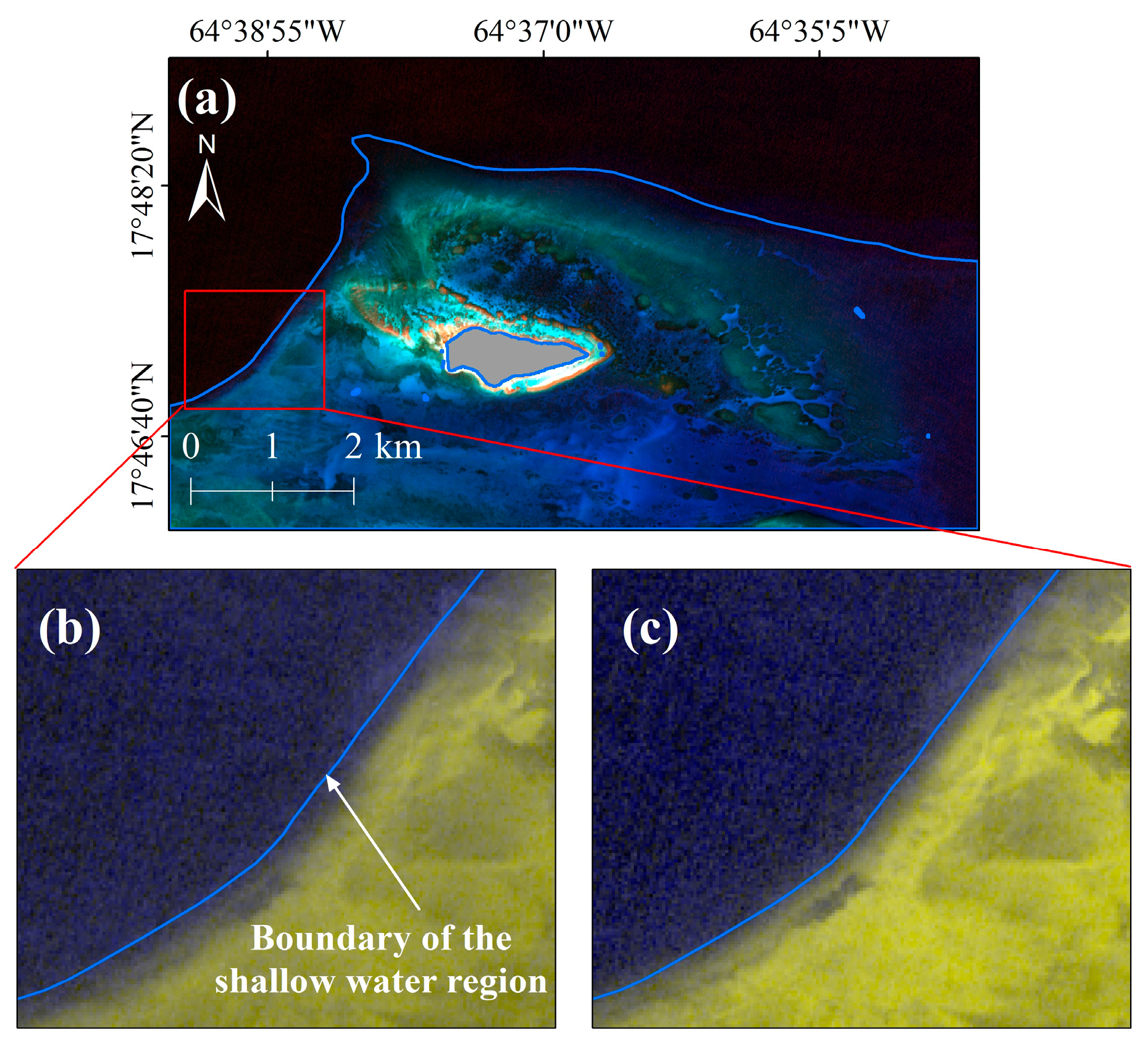
Using the Sentinel-2 image of Buck Island as an example (Figure 3a), the procedure for identifying shallow water regions through manual visual interpretation is described in detail. Two false-color composites were generated to enhance the contrast between shallow- and deep-water regions. Composite Image 1 (Figure 3b) was created by assigning Bands 3, 3, and 4 to the red, green, and blue channels, respectively, while Composite Image 2 (Figure 3c) was generated using Bands 2, 2, and 4 for the red, green, and blue channels, respectively. In both composites, shallow water regions appear yellowish-brown, whereas deep-water regions appear black. Based on this color contrast, the boundary between shallow- and deep-water regions was delineated by visually interpreting the interface between the yellowish-brown and black areas in Composite Image 1, with Composite Image 2 used as a reference to avoid misclassifying dark bottom types within shallow waters as deep-water regions. It should be noted that study areas vary in water transparency, bottom reflectance, and illumination conditions during image acquisition. Additionally, spectral confusion often occurs between dark substrates in shallow waters and pixels in deep-water regions. Consequently, some automated methods, such as threshold-based segmentation and supervised classification algorithms, demonstrate unstable performance across different sites. These methods frequently produce distortions, including “pseudo-shallow signals” in deep-water areas or misclassification of dark-bottom shallow waters as deep-water regions. In contrast, manual delineation based on false-color composite imagery offers more reliable identification of shallow-water boundaries under varying optical conditions. Because visual interpretation is inherently somewhat subjective, the visual criteria mentioned above were applied to ensure consistency in shallow-water boundary identification across the different study areas.

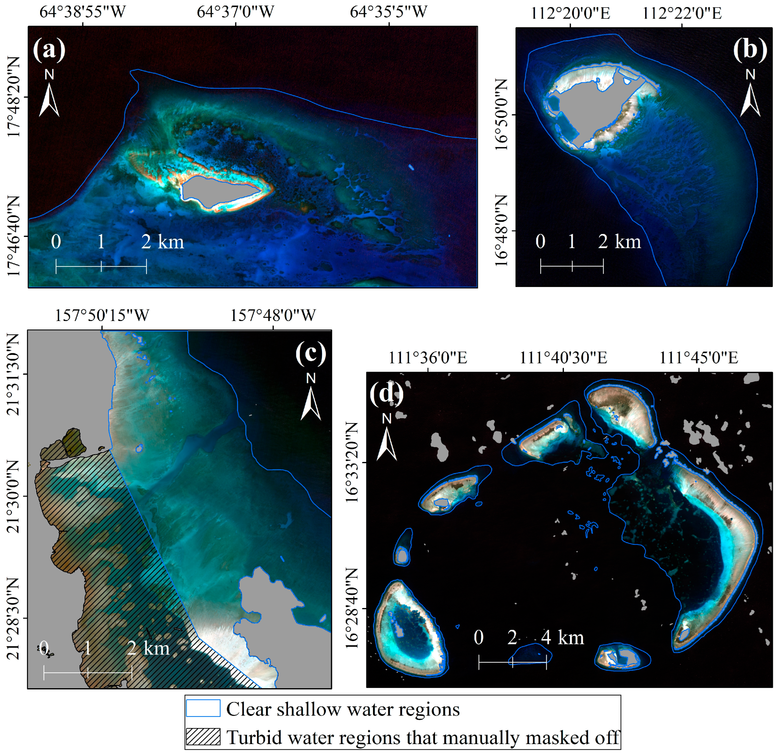
From the preprocessed imagery, the water-leaving reflectance (${\rho }_m$) can be directly obtained (as shown in Figure 4), which is subsequently used to calculate the observed remote sensing reflectance $R_{rs}^{obs}\left(={\rho }_m/\pi \right)$.

3. Methods

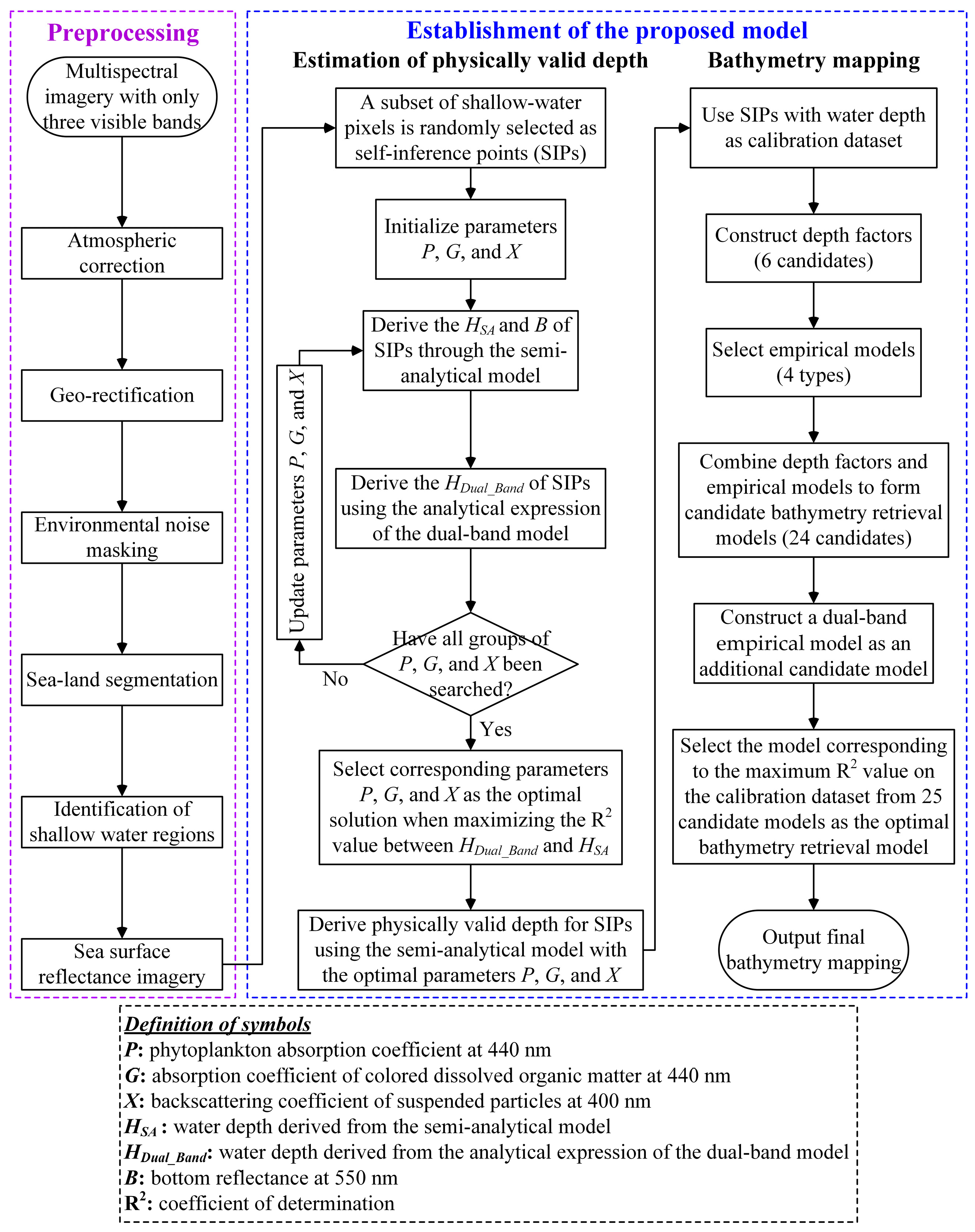
Figure 5 presents a flowchart of the proposed model, which consists of two main components. The first component explains how to integrate the semi-analytical model proposed by Lee et al. [25] with the analytical expression of the physics-based dual-band model developed by Chen et al. [33] to derive physically valid water depths for a subset of shallow-water pixels. The second component describes how to use the water depths from this subset as a calibration dataset to select the optimal model from 25 candidate bathymetry retrieval models, thereby calculating water depth information across the entire study area.

3.1. Traditional Physics-Based Approaches

3.1.1. Semi-Analytical Model

The core principle of the semi-analytical model for bathymetry retrieval is to describe the remote sensing reflectance of optically shallow water, $R_{rs}\left(\lambda \right)$, as a function of water depth, bottom reflectance, and the inherent optical properties of the water column [25]:

$$\begin{array}{c}{R}_{rs}\left(\lambda \right)=f\left(P, G,X,B,H,\lambda \right)\end{array}$$

(2)

where P is the absorption coefficient of phytoplankton at 440 nm, G is the absorption coefficient of yellow substances at 440 nm, X is the backscattering coefficient of suspended particles at 400 nm, B is the bottom reflectance at 550 nm, H is the water depth, and λ is the spectral wavelength.

The detailed radiative transfer equations are presented as follows:

$$\begin{array}{c}{R}_{rs}\left(\lambda \right)={\displaystyle \frac{0.52r_{rs}\left(\lambda \right)}{1-1.7r_{rs}\left(\lambda \right)}}\end{array}$$

(3)

$$\begin{array}{c}{r}_{rs}\left(\lambda \right)=r_{rs}^{dp}\left(\lambda \right)\left(1-e^{-\left(k_d\left(\lambda \right)+k_c\left(\lambda \right)\right)H}\right)+{\displaystyle \frac{{\rho }_b\left(\lambda \right)}{\pi }}{e}^{-\left(k_d\left(\lambda \right)+k_b\left(\lambda \right)\right)H}\end{array}$$

(4)

$$\begin{array}{c}{r}_{rs}^{dp}\left(\lambda \right)=\left(0.084+0.170{\displaystyle \frac{b_b\left(\lambda \right)}{a\left(\lambda \right)+b_b\left(\lambda \right)}}\right){\displaystyle \frac{b_b\left(\lambda \right)}{a\left(\lambda \right)+b_b\left(\lambda \right)}}\end{array}$$

(5)

$$\begin{array}{c}a\left(\lambda \right)=a_w\left(\lambda \right)+\left(a_0\left(\lambda \right)+a_1\left(\lambda \right)\ln P\right)P+G{e}^{-0.014\left(\lambda -440\right)}\end{array}$$

(6)

$$\begin{array}{c}{b}_b\left(\lambda \right)=b_{bw}\left(\lambda \right)+X{\left({\displaystyle \frac{400}{\lambda }}\right)}^{0.681}\end{array}$$

(7)

$$\begin{array}{c}{k}_d\left(\lambda \right)=\left(1+m_0{\theta }_s\right)a\left(\lambda \right)+m_1\left(1-\gamma {\displaystyle \frac{b_{bw}\left(\lambda \right)}{b_b\left(\lambda \right)}}\right)\left(1-m_2{e}^{-m_{3}a\left(\lambda \right)}\right)b_b\left(\lambda \right)\end{array}$$

(8)

$$\begin{array}{c}{k}_c\left(\lambda \right)={\displaystyle \frac{1}{\cos \left({\theta }_v\right)}}\left(a\left(\lambda \right)+b_b\left(\lambda \right)\right)\left[1.03{\left(1+2.4{\displaystyle \frac{b_b\left(\lambda \right)}{a\left(\lambda \right)+b_b\left(\lambda \right)}}\right)}^{0.5}\right]\end{array}$$

(9)

$$\begin{array}{c}{k}_b\left(\lambda \right)={\displaystyle \frac{1}{\cos \left({\theta }_v\right)}}\left(a\left(\lambda \right)+b_b\left(\lambda \right)\right)\left[1.04{\left(1+5.4{\displaystyle \frac{b_b\left(\lambda \right)}{a\left(\lambda \right)+b_b\left(\lambda \right)}}\right)}^{0.5}\right]\end{array}$$

(10)

$$\begin{array}{c}{\rho }_b\left(\lambda \right)=B{\rho }_{norm}\left(\lambda \right)\end{array}$$

(11)

where $r_{rs}\left(\lambda \right)$ denotes the subsurface remote sensing reflectance; $r_{rs}^{dp}\left(\lambda \right)$ represents the subsurface reflectance in deep waters; $k_d\left(\lambda \right)$ is the downwelling diffuse attenuation coefficient; $k_c\left(\lambda \right)$ is the upwelling radiance attenuation coefficient for water-column scattering; and $k_b\left(\lambda \right)$ is the upwelling radiance attenuation coefficient for bottom reflection. The symbols $a\left(\lambda \right)$ and $a_w\left(\lambda \right)$ denote the total absorption coefficient and the pure water absorption coefficient, respectively. The symbols $b_b\left(\lambda \right)$ and $b_{bw}\left(\lambda \right)$ denote the total backscattering coefficient and the pure water backscattering coefficient, respectively. The empirical coefficients $a_0\left(\lambda \right)$ and $a_1\left(\lambda \right)$ are defined in Reference [24]. The angles ${\theta }_s$ and ${\theta }_v$ represent the subsurface solar zenith angle and the subsurface satellite viewing angle, respectively. The empirical constants $m_0$, $m_1$, $m_2$, $m_3$, and $\gamma$ are independent of spectral wavelength and water properties, with values of 0.005, 4.26, 0.52, 10.8, and 0.265, respectively. The symbol ${\rho }_b\left(\lambda \right)$ is the bottom reflectance, and ${\rho }_{norm}\left(\lambda \right)$ is the normalized bottom reflectance.

The remote sensing reflectance for specific bands, $R_{rs}\left({Band}_i\right)$, is then approximated using the spectral response function of the satellite sensor:

$$\begin{array}{c}{R}_{rs}\left({Band}_i\right)={\displaystyle \frac{{\int }_{{\lambda }_{lower}}^{{\lambda }_{upper}}{R_{rs}\left(\lambda \right)SRF}_i\left(\lambda \right)\mathrm{d}\mathsf{\lambda }}{{\int }_{{\lambda }_{lower}}^{{\lambda }_{upper}}{SRF}_i\left(\lambda \right)\mathrm{d}\mathsf{\lambda }}}\end{array}$$

(12)

where ${Band}_i$ and ${SRF}_i\left(\lambda \right)$ denote the spectral band and its corresponding spectral response function.

The cost function for optimization is defined as follows:

$$\begin{array}{c}\mathrm{cost} \mathrm{function}={\displaystyle \frac{\sqrt{\sum _{i=1}^N{\left[R_{rs}\left({Band}_i\right)-R_{rs}^{obs}\left({Band}_i\right)\right]}^2}}{\sum _{i=1}^N{R}_{rs}^{obs}\left({Band}_i\right)}}\end{array}$$

(13)

where N is the number of bands used for spectral matching, the Sequential Least Squares Programming (SLSQP) algorithm from the Python v3.10.14 SciPy v1.15.3 library was employed to minimize this cost function and simultaneously retrieve the parameters P, G, X, B, and H.

3.1.2. Physics-Based Dual-Band Model

The physics-based dual-band model, proposed by Chen et al. in 2019, is an innovative approach for bathymetry retrieval using multispectral imagery [33,36,39]. All unknown parameters in the model are estimated from sampled pixels within remote sensing images, thereby eliminating the need for in situ bathymetric data. The analytical expression for the dual-band model is derived by applying vector addition to the single-band models corresponding to the blue and green bands, as follows:

$$\begin{array}{c}R=-gH+\ln r_b^{*}\end{array}$$

(14)

$$\begin{array}{c}\stackrel{⃑}{\alpha }·\stackrel{⃑}{R}=\stackrel{⃑}{\alpha }·\ln \stackrel{⃑}{r_b}-\left(\stackrel{⃑}{\alpha }·\stackrel{⃑}{g}\right)H\end{array}$$

(15)

$$\begin{array}{c}H=\left[{\displaystyle \frac{-1/g_2}{g_1/g_2\ast {\alpha }_1+{\alpha }_2}}\right]\ast \left[{\alpha }_1{R}_1+{\alpha }_2{R}_2-\left({\alpha }_1\ln r_{b1}^{*}+{\alpha }_2\ln r_{b2}^{*}\right)\right]\end{array}$$

(16)

where H is the water depth, $g$ is the diffuse attenuation coefficient, $R=\ln \left(r_{rs}-r_{rs}^{dp}\right)$, and $\ln r_b^{\mathrm{*}}=\ln \left({\rho }_b/\pi -r_{rs}^{dp}\right)$. The vectors are defined as $\stackrel{⃑}{R}=\left[R_1,R_2\right]$, $\ln \stackrel{⃑}{r_b}=\left[\ln r_{b1}^{\mathrm{*}},\ln r_{b2}^{\mathrm{*}}\right]$, $\stackrel{⃑}{g}=\left[g_1,g_2\right]$, and $\stackrel{⃑}{\alpha }=\left[{\alpha }_1,{\alpha }_2\right]$, where $\stackrel{⃑}{\alpha }$ is the optimal band-rotation coefficient unit vector that minimizes the influence of bottom type on bathymetry retrieval. Subscripts 1 and 2 refer to the blue and green bands, respectively.

Assuming that the water depths of two adjacent pixels are approximately equal, a set of $R_1$~$R_2$ pixel pairs can be randomly selected from the imagery. These pixel pairs must be located at the boundaries separating different bottom types that occur at varying depths. The vector $\stackrel{⃑}{\alpha }$ is then estimated by minimizing the following objective function:

$$\begin{array}{c}f\left({\alpha }_1,{\alpha }_2\right)=\mathrm{argmin}\left[{\displaystyle \sum _{j=1}^n}{\left({\left|\left({\alpha }_1{R}_1^A+{\alpha }_2{R}_2^A\right)-\left({\alpha }_1{R}_1^C+{\alpha }_2{R}_2^C\right)\right|}_j\right)}^2\right]\end{array}$$

(17)

where $j$ denotes a specific adjacent pixel pair, $n$ is the number of pixel pairs, and $\left|\stackrel{⃑}{\alpha }\right|=1$. Superscripts A and C refer to the two pixels within a pair, representing different bottom types.

As reported in Reference [33], the mean value of ${\alpha }_1{R}_1+{\alpha }_2{R}_2$, derived from pixels of different bottom types near the waterline, serves as an estimate of the bottom parameter ${\alpha }_1\ln r_{b1}^{\mathrm{*}}+{\alpha }_2\ln r_{b2}^{\mathrm{*}}$. The ratio $g_1/g_2$ can be regarded as the slope of the regression equation constructed from the $R_1$~$R_2$ dataset collected for the same bottom type at different depths. The green-band diffuse attenuation coefficient $g_2$ is calculated using the latest version of the Quasi-Analytical Algorithm (QAA_v6).

3.1.3. L-S Model

Xia et al. proposed a hybrid approach that combines a logarithmic ratio model with a semi-analytical model, referred to as the L-S model, which eliminates the need for in situ bathymetric data [32]. Directly solving for the optimal set of parameters P, G, X, B, and H in the semi-analytical model (as described in Section 3.1.1) is often ill-conditioned when only three visible bands are available. To address this issue, the L-S model constrains the semi-analytical retrieval using a logarithmic ratio relationship. For each selected pixel, the water depth is expressed as follows:

$$\begin{array}{c}{H}_{SA}=m_1{\displaystyle \frac{\mathrm{l}\mathrm{n}\left(1000R_{rs}\left(Blue\right)\right)}{\mathrm{l}\mathrm{n}\left(1000R_{rs}\left(Green\right)\right)}}-m_0\end{array}$$

(18)

where $H_{SA}$ is the water depth derived from the semi-analytical model, $R_{rs}\left(Blue\right)$ and $R_{rs}\left(Green\right)$ represent the remote sensing reflectances in the blue and green bands, respectively, and $m_0$ and $m_1$ are empirical fitting coefficients.

All combinations of P, G, and X are iteratively input into the semi-analytical model to solve for the corresponding B and H. During the iteration process, when the correlation between $H_{SA}$ and $\frac{\mathrm{l}\mathrm{n}\left(1000R_{rs}\left(Blue\right)\right)}{\mathrm{l}\mathrm{n}\left(1000R_{rs}\left(Green\right)\right)}$ reaches its maximum, the associated values of B and H are considered optimal. The corresponding P, G, and X values are then regarded as the best representation of the prevailing water conditions. Finally, the calibrated logarithmic ratio model is applied to estimate bathymetry across the entire study area.

3.2. Establishment of the Novel Semi-Analytical-Empirical Hybrid Model

3.2.1. Model Overview

Traditional semi-analytical models involve at least five unknown parameters, so solving them using only three visible bands from a multispectral image often results in multiple numerical solutions and, consequently, unstable depth retrieval outcomes. To address this issue, it is necessary to reduce the number of unknowns in the semi-analytical model. In regions of relatively small geographic extent, water clarity tends to be approximately uniform, allowing the water-optical parameters P, G, and X to be treated as constants. By assigning the same values of P, G, and X to all water pixels within the area, the number of unknowns in the semi-analytical model is effectively reduced, making it applicable to nearly any multispectral image. Therefore, determining the optimal values of P, G, and X is crucial when applying the semi-analytical model to imagery containing only three visible bands.

If P, G, and X are held constant within a given area, an analytical expression for a dual-band model can be derived from the shallow-water radiative transfer equation. This derivation explicitly reveals the relative relationship among the depths of different pixels, as described by the dual-band model. However, traditional semi-analytical models solve for each pixel independently and in parallel, without considering this relationship. By utilizing the analytical expression from the dual-band model, the solution processes of the semi-analytical model for different pixels within the same image can be linked, thereby ensuring successful bathymetry retrieval.

Specifically, all combinations of the parameters P, G, and X are exhaustively enumerated, and each combination is input into the semi-analytical model to compute the corresponding bottom reflectance B and depth H. Each set of parameters (P, G, X, B, H) is considered a numerical solution of the semi-analytical model because it satisfies the condition $R_{rs}\left({Band}_i\right)\approx R_{rs}^{obs}\left({Band}_i\right)$. For each combination of P, G, and X, the analytical depth is then calculated using the dual-band model. For each combination of P, G, and X, the difference between the depth calculated by the semi-analytical model and the depth analytically determined by the dual-band model is evaluated. The combination that minimizes this difference is selected as the optimal set of parameters. These optimal values of P, G, and X effectively represent the optical properties of the water in the area, and the depth obtained by inputting this set into the semi-analytical model is considered physically valid. Once physically valid depths for a subset of shallow-water pixels are obtained, these depths are used as a calibration dataset to determine the optimal combination of a depth factor and an empirical method, collectively forming the optimal bathymetry retrieval model. This model is then applied to calculate water depth across the entire study area.

3.2.2. Determining Physically Valid Depth by Combining Semi-Analytical and Dual-Band Models

The proposed model initially quantifies the relative relationships among the depths of different pixels by integrating the semi-analytical model with the dual-band model. This relative relationship is then used as a constraint to identify physically valid depths from the multiple numerical solutions provided by the semi-analytical model for a subset of shallow-water pixels. The detailed estimation process for obtaining valid depths for this subset of shallow-water pixels is as follows:

• Step 1: Randomly select a specific number of pixels (e.g., 200) within the shallow-water region. These pixels serve as Self-Inference Points (SIPs) to assess whether the relative depth relationships among pixels are maintained.
• Step 2: Set the initial values of the parameters P, G, and X (e.g., P = 0.005, G = 0.005, X = 0.003).
• Step 3: Input the initial values of P, G, and X into the semi-analytical model to derive the corresponding bottom reflectance B and depth H for each SIP.
• Step 4: For each SIP, the semi-analytical model produces retrieved values of B and H. Additionally, the depth of each SIP can be expressed analytically using the dual-band model:

$$\begin{array}{c}{H}_{Dual\_Band}=\left[{\displaystyle \frac{-1/g_2}{g_1/g_2\ast {\alpha }_1+{\alpha }_2}}\right]\ast \left[{\alpha }_1{R}_1+{\alpha }_2{R}_2-\left({\alpha }_1\ln r_{b1}^{*}+{\alpha }_2\ln r_{b2}^{*}\right)\right]\end{array}$$

(19)

where $H_{Dual\_Band}$ is the depth analytically derived from the dual-band model, and the symbols $R_1$, $R_2$, ${\alpha }_1$, ${\alpha }_2$, $g_1$, $g_2$, $\ln r_{b1}^{\mathrm{*}}$, and $\ln r_{b2}^{\mathrm{*}}$ are defined as in Equation (16) of the main text. In this model, the parameters $g_1$, $g_2$, and the combination ${\alpha }_1\ln r_{b1}^{\mathrm{*}}+{\alpha }_2\ln r_{b2}^{\mathrm{*}}$ are not estimated using the method described in Section 3.1.2; instead, they are treated as constants that depend on P, G, and X, with unknown values. This adjustment is intended to prevent the physics-based dual-band model from being affected by non-ideal deep-water sample pixels and to enable the model to be applied to waters without a waterline.

From previous research, $g\left(\lambda \right)=k_d\left(\lambda \right)+\left(k_b\left(\lambda \right)+k_c\left(\lambda \right)\right)/2$. Thus, the diffuse attenuation coefficient $g\left(\lambda \right)$ can be expressed as a function of the parameters P, G, and X, i.e., $g\left(\lambda \right)=f\left(P,G,X,\lambda \right)$. Using the sensor spectral response function ${SRF}_i\left(\lambda \right)$, the band-averaged diffuse attenuation coefficient $g_i$ for the ith band can be approximated by:

$$\begin{array}{c}{g}_i={\displaystyle \frac{{\int }_{{\lambda }_{lower}}^{{\lambda }_{upper}}g\left(\lambda \right){SRF}_i\left(\lambda \right)\mathrm{d}\mathsf{\lambda }}{{\int }_{{\lambda }_{lower}}^{{\lambda }_{upper}}{SRF}_i\left(\lambda \right)\mathrm{d}\mathsf{\lambda }}}\end{array}$$

(20)

The values of $g_1$ and $g_2$ for the blue and green bands, respectively, are obtained from Equation (20). Similarly, from Equation (11) in the main text, it is known that the bottom reflectance, ${\rho }_b\left(\lambda \right)$, is a function of the parameter B; that is, ${\rho }_b\left(\lambda \right)=f\left(B,\lambda \right)$. For each SIP, using ${SRF}_i\left(\lambda \right)$, the bottom reflectance ${\rho }_{b,i}$ in the ith band can be approximated by:

$$\begin{array}{c}{\rho }_{b,i}={\displaystyle \frac{{\int }_{{\lambda }_{lower}}^{{\lambda }_{upper}}{\rho }_b\left(\lambda \right){SRF}_i\left(\lambda \right)\mathrm{d}\mathsf{\lambda }}{{\int }_{{\lambda }_{lower}}^{{\lambda }_{upper}}{SRF}_i\left(\lambda \right)\mathrm{d}\mathsf{\lambda }}}\end{array}$$

(21)

Using the values of ${\rho }_{b,i}$, the expression ${\alpha }_1\ln r_{b1}^{\mathrm{*}}+{\alpha }_2\ln r_{b2}^{\mathrm{*}}$ is calculated for each SIP under the current combination of P, G, and X. The average of all these ${\alpha }_1\ln r_{b1}^{\mathrm{*}}+{\alpha }_2\ln r_{b2}^{\mathrm{*}}$ values from the SIPs is then taken as the estimate of this bottom-related parameter. At this stage, all unknowns in the analytical expression of the dual-band model (Equation (19)) are determined, enabling the calculation of $H_{Dual\_Band}$ for all SIPs under the current combination of P, G, and X.

For convenience, denote the depth obtained from the semi-analytical model as $H_{SA}$. For each SIP, different sets of parameters P, G, and X produce varying values of $H_{SA}$ and $H_{Dual\_Band}$. When the correct values of P, G, and X are selected, the difference between $H_{SA}$ and $H_{Dual\_Band}$ for each SIP should be close to zero. Theoretically, if P, G, and X are accurate, the coefficient of determination R² between $H_{SA}$ and $H_{Dual\_Band}$ across all SIPs should approach 1. Conversely, if P, G, and X are incorrect, R² should approach 0.

• Step 5: Adjust parameters P, G, and X according to their predefined ranges and step sizes, and repeat step 4 until all combinations of P, G, and X have been searched. This is a brute-force search process. When the coefficient of determination R² between $H_{SA}$ and $H_{\mathit{Dual}\_\mathit{Band}}$ reaches its maximum value, the corresponding values of P, G, and X are considered optimal. Notably, the ranges of P, G, and X are determined with References [32,34], and their search step sizes are empirical values chosen to balance accuracy and computational efficiency. The parameter ranges and step sizes of the model are provided in

  Table 1. Parameter ranges and search step sizes for the model.

  Parameter	Initial Value	Range	Step
  P	0.005	0.005–0.1	0.002
  G	0.005	0.005–0.03	0.002
  X	0.003	0.003–0.15	0.002
  B	0.5	0.002–1.0
  H	3	0–30

  .

Here, we provide a detailed explanation of the reasons for selecting the brute-force search method, which is used for determining the globally optimal solution for the parameters P, G, and X. Gradient-based optimization methods are inherently unsuitable for optimizing our objective function—used to find the values of P, G, and X that maximize the R² value between $H_{SA}$ and $H_{Dual\_Band}$—due to the function’s complex structure and potential non-differentiability. Although heuristic algorithms (e.g., Genetic Algorithm, Particle Swarm Optimization, and Bayesian Optimization) could be considered as alternatives, they do not guarantee convergence to the global optimum, and their performance is often sensitive to hyperparameter tuning. Given the critical importance of identifying the globally optimal parameters P, G, and X for accurate bathymetry retrieval, and considering that the search space involves only three dimensions (P, G, and X), a brute-force grid search strategy was adopted. While computationally intensive, this approach exhaustively explores the predefined parameter ranges, is embarrassingly parallelizable, and, most importantly, provides a valid guarantee of finding the global optimum within the discretized search space. This guarantee is paramount for the reproducibility and reliability of our retrieval method.

• Step 6: After determining the optimal P, G, and X parameters, retrieve the depths of all SIPs using the semi-analytical model with these parameters.

3.2.3. Bathymetry Mapping Using the Optimal Bathymetry Retrieval Model

After obtaining the valid depths for the SIPs, these depths are used as a calibration dataset. An optimal bathymetry retrieval model, which enables depth estimation across the entire study area, is then developed by selecting the best combination of a depth factor and an empirical method. Numerous depth factors and empirical methods are available; even pairing the same factor with different methods or pairing different factors with the same method can produce varying retrieval results. Therefore, to identify the optimal bathymetry retrieval model in practice, it is essential to systematically compare the performance of all possible combinations of depth factors and empirical methods.

To construct depth factors suitable for Case-I water environments, we select three physical quantities that contain depth information: the remote sensing reflectance $R_{rs}\left({Band}_i\right)$, the subsurface remote sensing reflectance $r_{rs}\left({Band}_i\right)$, and the inherent optical parameter $u\left({Band}_i\right)$. These quantities are related as follows: $r_{rs}\left({Band}_i\right)=\frac{R_{rs}\left({Band}_i\right)}{0.52+1.7R_{rs}\left({Band}_i\right)}$, $u\left({Band}_i\right)=\frac{-p_0+\sqrt{{\left(p_0\right)}^2+4p_1\ast r_{rs}\left({Band}_i\right)}}{2p_1}$ where $p_0=0.0895$ and $p_1=0.1247$. Next, we form ratios and logarithmic ratios between the blue and green bands of these quantities, generating a total of six depth factors as follows: $R_{rs}\left(Blue\right)/R_{rs}\left(Green\right)$, $r_{rs}\left(Blue\right)/r_{rs}\left(Green\right)$, $u\left(Blue\right)/u\left(Green\right)$, $\mathit{ln}\left(1000R_{rs}\left(Blue\right)\right)/\mathit{ln}\left(1000R_{rs}\left(Green\right)\right)$, $\mathit{ln}\left(1000r_{rs}\left(Blue\right)\right)/\mathit{ln}\left(1000r_{rs}\left(Green\right)\right)$ and $\mathit{ln}\left(1000u\left(Blue\right)\right)/\mathit{ln}\left(1000u\left(Green\right)\right)$.

Given that the number of SIPs is only on the order of a few hundred, the calibration dataset remains relatively small; therefore, complex machine learning methods that may lead to overfitting are not employed. In practice, the linear relationship between water depth and the logarithmic ratio of the blue and green bands is generally valid only within a certain shallow depth range, beyond which the relationship becomes nonlinear. Moreover, nonlinearity may arise not only in the logarithmic ratio factor but also in other depth factors derived from the blue and green bands. To more accurately characterize the potentially complex relationship between water depth and various depth factors, four classical empirical models commonly referenced in previous studies are adopted for fitting: a linear model (Equation (22)), a quadratic polynomial model (Equation (23)), a power model (Equation (24)), and an exponential model (Equation (25)) [40].

$$\begin{array}{c}H=m_0+m_{1}x\end{array}$$

(22)

$$\begin{array}{c}H=m_0+m_{1}x+m_2{x}^2\end{array}$$

(23)

$$\begin{array}{c}H=m_0+m_1{x}^{m_2}, m_2>0\end{array}$$

(24)

$$\begin{array}{c}H=m_0+m_1{m_2}^x, m_2>1\end{array}$$

(25)

where H denotes the water depth, x is a depth factor, and $m_0$, $m_1$, and $m_2$ are adjustable parameters.

By combining the six depth factors described above with the four empirical models, a total of 24 candidate bathymetry retrieval models are obtained. In addition, the widely used dual-band empirical method is included in the evaluation set, resulting in 25 candidate models for identifying the optimal bathymetric retrieval approach. For each model, the coefficient of determination R² is calculated using the calibration dataset, and the model yielding the highest R² is selected to estimate water depth across the entire study area.

3.3. Accuracy Evaluation Indicators

In this paper, the root-mean-square error (RMSE), mean absolute error (MAE), and coefficient of determination (R²) are used to evaluate the accuracy of bathymetry estimation results. RMSE and MAE quantify the errors between the derived and measured bathymetry; smaller RMSE and MAE values indicate more accurate bathymetry estimations. R² reflects the degree of fit between the derived and measured bathymetry, with values ranging from 0 to 1. The closer the R² value is to 1, the better the bathymetry estimation results.

$$\begin{array}{c}\mathrm{RMSE}=\sqrt{{\displaystyle \frac{\sum _{i=1}^n{\left(y_i-y_i^T\right)}^2}{n}}}\end{array}$$

(26)

$$\begin{array}{c}MAE={\displaystyle \frac{\sum _{i=1}^n\left|y_i-y_i^T\right|}{n}}\end{array}$$

(27)

$$\begin{array}{c}{\mathrm{R}}^2={\displaystyle \frac{\sum _{i=1}^n{\left(y_i-\overline{y}\right)}^2}{\sum _{i=1}^n{\left(y_i^T-\overline{y}\right)}^2}}\end{array}$$

(28)

where $y_i$ and $y_i^T$ represent the derived and measured bathymetry of the $i$-th validation sample, respectively, $\overline{y}$ denotes the average of the measured bathymetry across all validation samples, and $n$ indicates the total number of validation samples.

4. Results

4.1. Selection Results of the Optimal Bathymetry Retrieval Model

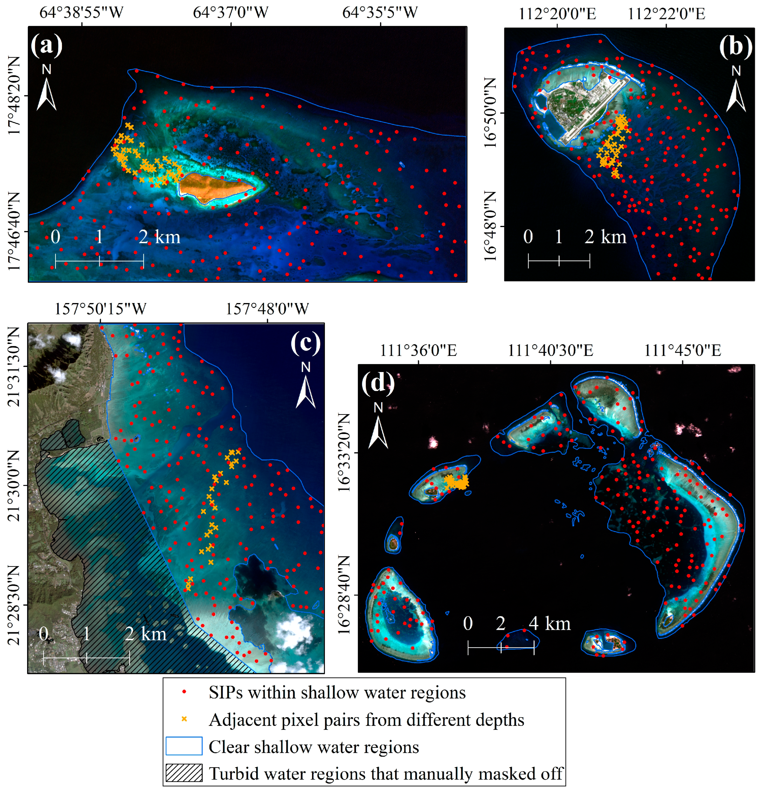
In each of the four study areas, two types of sampled pixels were selected from the preprocessed multispectral images: (1) adjacent pixel pairs located at the boundaries of different bottom types at varying depths (following the same selection strategy as the physics-based dual-band model), and (2) SIPs randomly distributed within the shallow-water regions. When selecting SIPs, a large minimum spacing between points was enforced to prevent spatial clustering. The spatial distribution of the sampled pixels is illustrated in Figure 6.

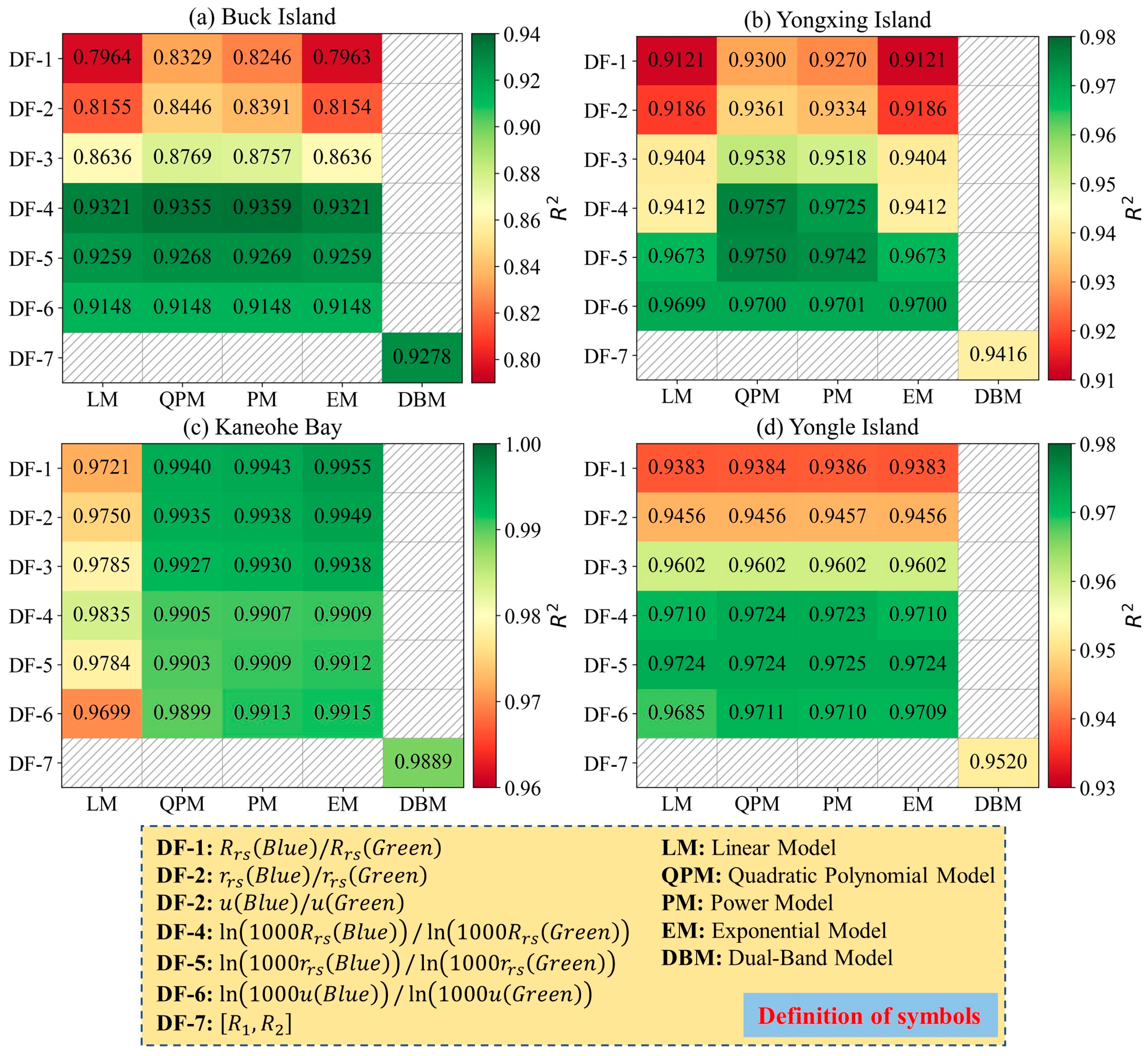
Using the selected adjacent pixel pairs, the optimal band-rotation coefficient unit vectors $\left[{\alpha }_1,{\alpha }_2\right]$ were estimated for each study area. The obtained values were [−0.545, 0.839] for Buck Island, [−0.550, 0.835] for Yongxing Island, [−0.665, 0.747] for Kaneohe Bay, and [−0.609, 0.793] for Yongle Atoll. Subsequently, the semi-analytical model and the dual-band model were jointly applied to calculate the physically valid depths of the SIPs, which were then used as a calibration dataset. A total of 25 candidate bathymetry retrieval models were constructed. The coefficient of determination (R²) for each model was calculated based on the calibration dataset. The R² values for all 25 models in each region are presented in Figure 7.

Based on the results presented in Figure 6, the optimal retrieval model for each study area was determined, and the corresponding outcomes are summarized in

Table 2. Results of the selected optimal bathymetry retrieval model.

Model Option	Buck Island	Yongxing Island	Kaneohe Bay	Yongle Atoll
Optimal depth factor x	$\ln \left(1000R_{rs}\left(Blue\right)\right)/\ln \left(1000R_{rs}\left(Green\right)\right)$	$\ln \left(1000R_{rs}\left(Blue\right)\right)/\ln \left(1000R_{rs}\left(Green\right)\right)$	$R_{rs}\left(Blue\right)/R_{rs}\left(Green\right)$	$\ln \left(1000r_{rs}\left(Blue\right)\right)/\ln \left(1000r_{rs}\left(Green\right)\right)$
Optimal empirical model	Power model	Quadratic polynomial model	Exponential model	Power model
Model expression	$H=-144.7182+148.0490x^{0.2381}$	$H=-38.4748+50.6708x-9.2318x^2$	$H=-6.4351+3.3332\times {2.8527}^x$	$H=-49.4724+52.9514x^{1.1093}$

.

4.2. Bathymetric Map

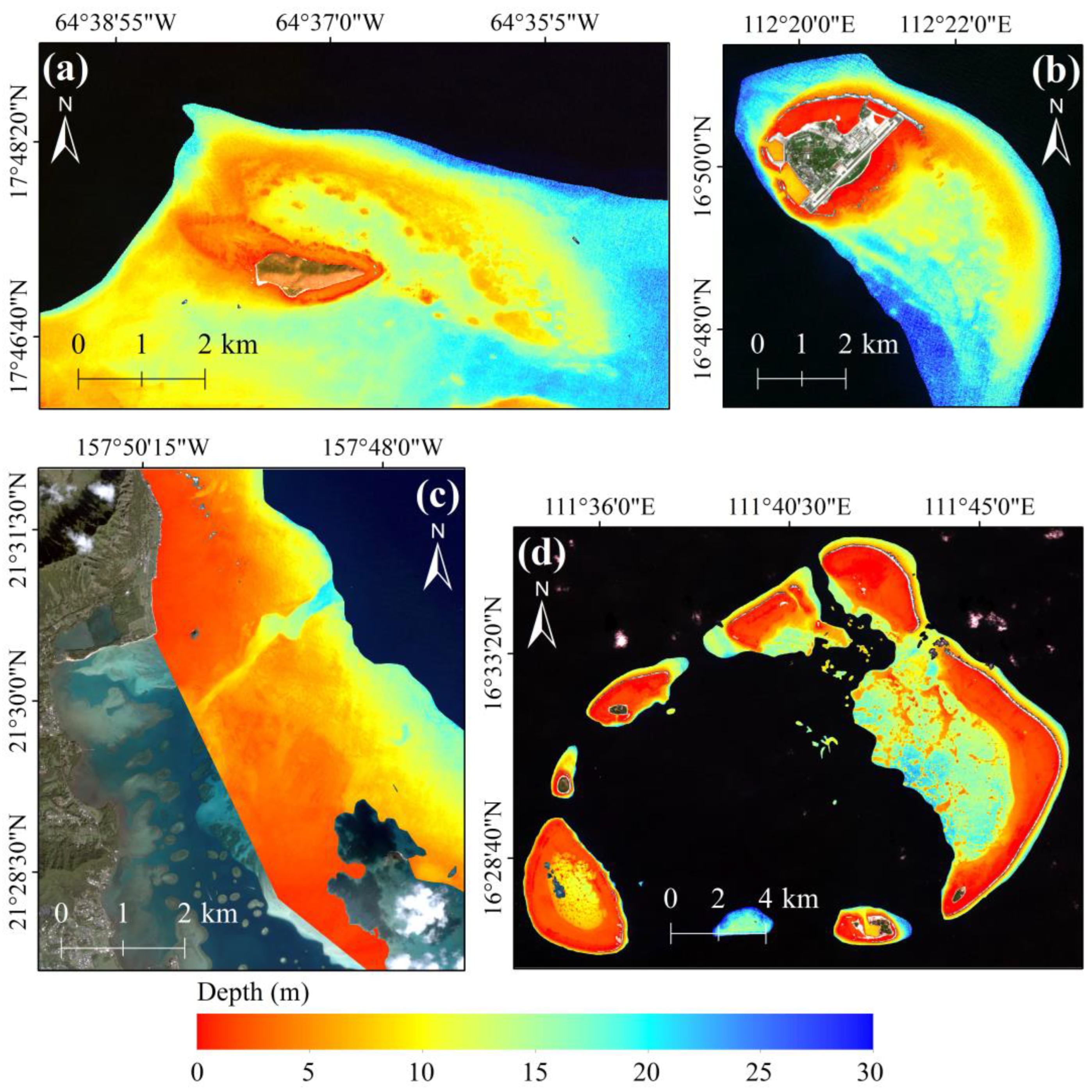
The optimal models identified above were subsequently applied to the full multispectral images of the four study areas to generate complete bathymetric maps. The resulting maps are presented in Figure 8. Visually, the bathymetric maps produced by the proposed model clearly depict the underwater terrain, including gullies and undulations, and capture detailed seafloor features in shallow-water regions. Each map exhibits a consistent trend of increasing depth moving outward from the reef platform, accurately reflecting the actual depth distribution. This demonstrates that the proposed model can generate spatially continuous depth estimates from multispectral imagery containing only three visible bands, without relying on any in situ depth measurements. The objective accuracy of these estimates will be rigorously evaluated in Section 4.3 using independent in situ data.

4.3. Overall Accuracy Evaluation

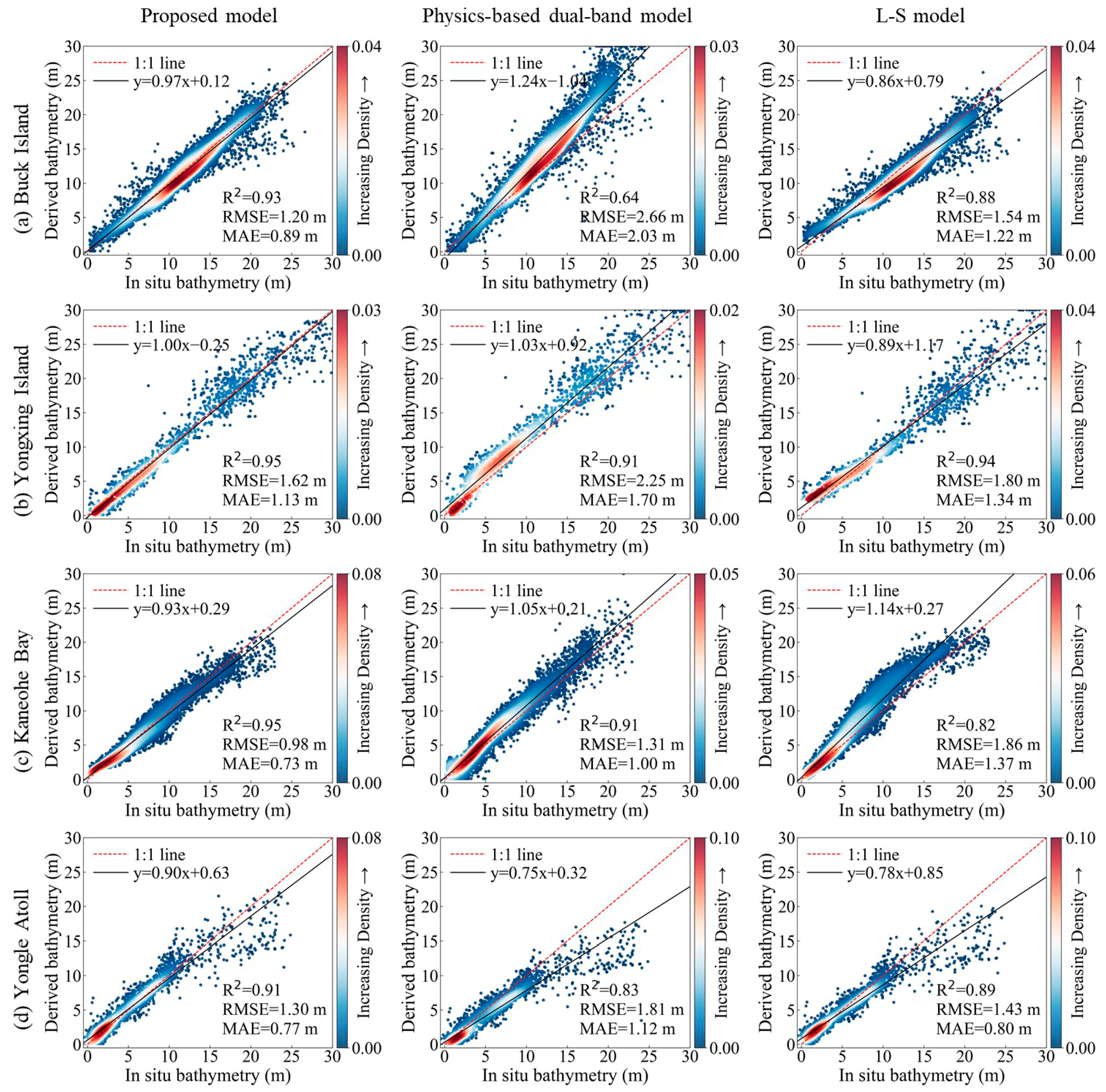
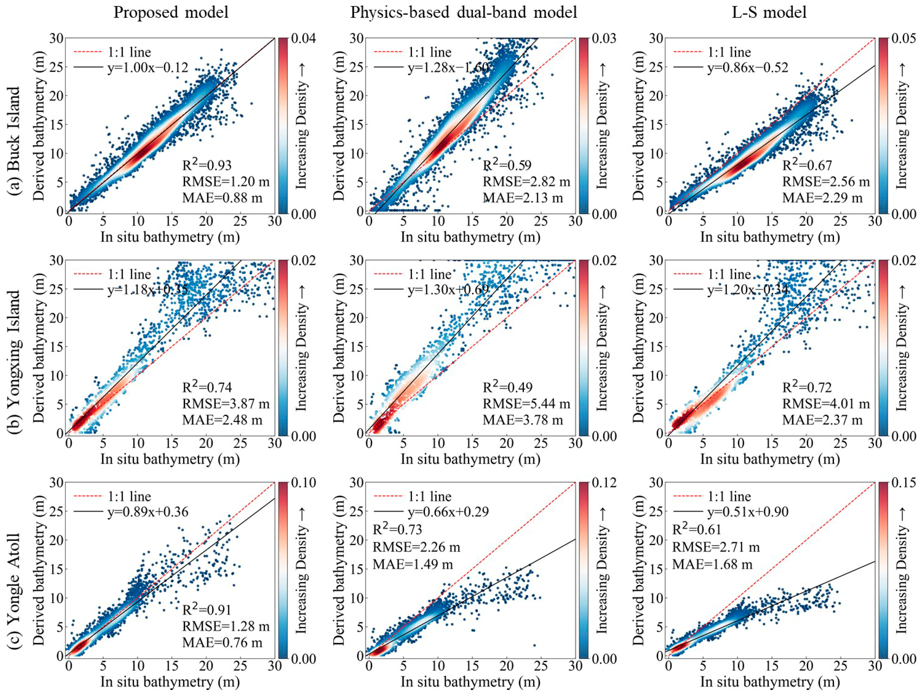
To systematically evaluate the performance of the proposed model in Case-I waters, its retrieval accuracy was compared with that of two widely used methods: the physics-based dual-band model and the L-S model. This comparison was conducted by plotting the derived bathymetry against the in situ bathymetry for each model (see Figure 9) and by calculating the RMSE, MAE and R² values. As shown in Figure 9, the proposed model exhibits a clear accuracy advantage across all study areas. The quantitative comparison results are summarized below:

• Buck Island: The proposed model demonstrated excellent performance, achieving an RMSE of 1.20 m, an MAE of 0.89 m, and an R² of 0.93. Compared to the physics-based dual-band model, the RMSE decreased by 55%, the MAE by 56%, and the R² increased by 0.29. Relative to the L-S model, the RMSE was 22% lower, the MAE was 27% lower, and the R² improved by 0.05.
• Yongxing Island: The proposed model achieved an RMSE of 1.62 m, an MAE of 1.13 m, and an R² value of 0.95. This represents a 28% reduction in RMSE and a 34% reduction in MAE compared to the physics-based dual-band model, along with a 0.04 increase in R². Compared to the L-S model, the RMSE and MAE decreased by 10% and 16%, respectively, while the R² improved by 0.01.
• Kaneohe Bay: The proposed model achieved an RMSE of 0.98 m, an MAE of 0.73 m, and an R² value of 0.95. It outperformed the physics-based dual-band model, exhibiting 25% and 27% reductions in RMSE and MAE, respectively, along with a 0.04 increase in R². Compared to the L-S model, the improvements were even more significant: RMSE and MAE both decreased by 47%, while R² increased by 0.13.
• Yongle Atoll: The proposed model achieved an RMSE of 1.30 m, an MAE of 0.77 m, and an R² of 0.91. Compared to the physics-based dual-band model, the RMSE and MAE were reduced by 28% and 31%, respectively, while the R² increased by 0.08. Compared to the L-S model, it demonstrated a 9% lower RMSE, a 4% lower MAE, and a 0.02 higher R².

These results indicate that the proposed model consistently achieves superior bathymetry retrieval accuracy across all study areas. Its derived bathymetry closely matches the in situ measurements and clearly outperforms both the physics-based dual-band model and the L-S model, neither of which utilize in situ depth data.

4.4. Accuracy Evaluation in Different Depth Intervals

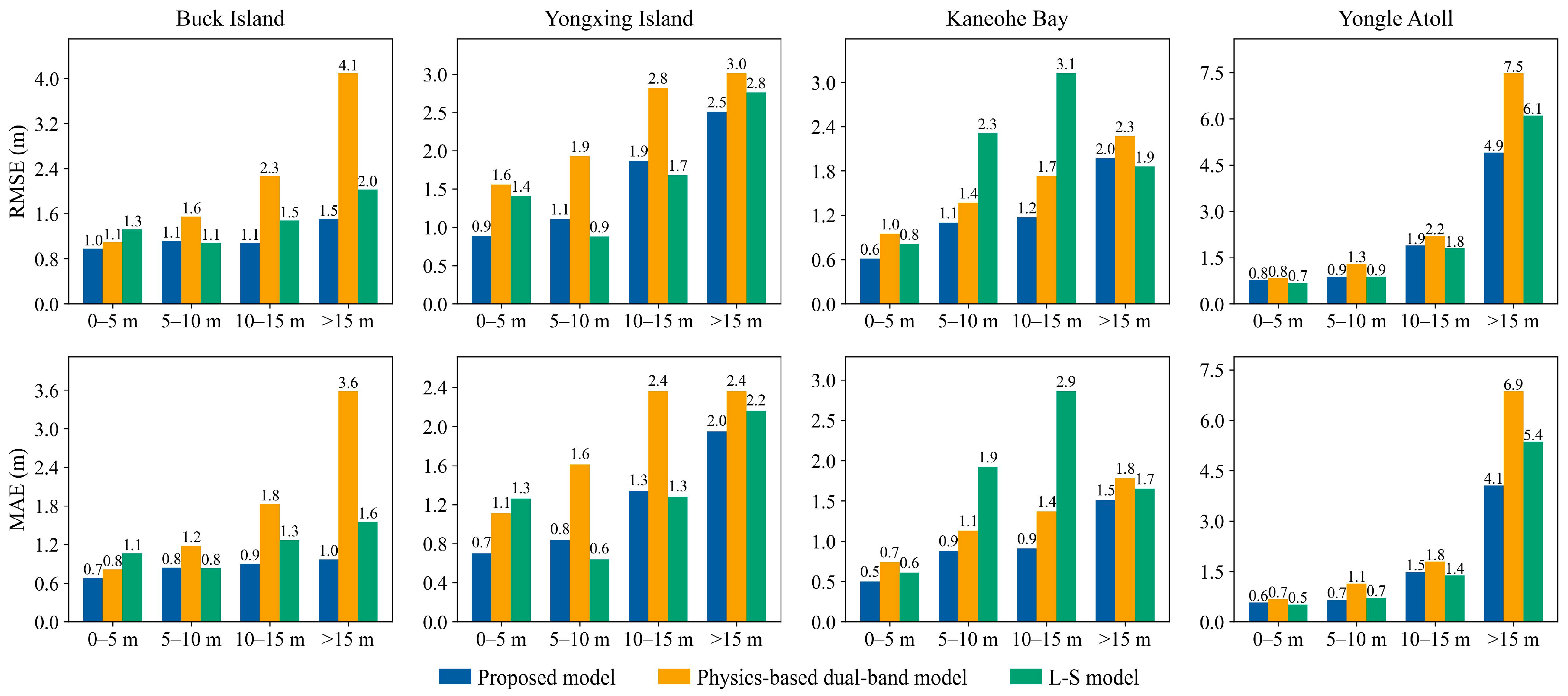
Figure 9 shows that the three models exhibit varying accuracies across different depth ranges. To quantify these differences, the measured depths were divided into four typical intervals (0–5 m, 5–10 m, 10–15 m, and >15 m), and the RMSE and MAE values for each model were calculated within each interval. The results are presented in Figure 10. As shown in Figure 10, with increasing water depth, the RMSE and MAE of the three models in each study area generally show an increasing trend. Furthermore, the proposed model demonstrates a clear accuracy advantage across all depth intervals in each study area. Detailed results are provided below:

• Buck Island: The proposed model achieves the highest retrieval accuracy across all depth intervals. In the 0–5 m interval, its performance is comparable to that of the physics-based dual-band model, with RMSE and MAE differences within 0.1 m. However, at depths greater than 5 m, the proposed model significantly outperforms the physics-based dual-band model, reducing RMSE by approximately 0.5–2.6 m and MAE by 0.4–2.6 m. Compared to the L-S model, the proposed model performs similarly within the 5–10 m interval but demonstrates clear advantages in both the 0–5 m and >10 m intervals, reducing RMSE by approximately 0.3–0.5 m and MAE by 0.4–0.6 m.
• Yongxing Island: The proposed model achieves the highest or second-highest retrieval accuracy across all depth intervals. Specifically, in the 0–5 m and >15 m intervals, its accuracy is significantly superior to that of the other two models, with RMSE reductions of at least 0.3 m and MAE reductions of at least 0.2 m. Within the 5–15 m interval, the proposed model performs slightly worse than the L-S model; however, it clearly outperforms the physics-based dual-band model, achieving reductions in RMSE and MAE of at least 0.8 m.
• Kaneohe Bay: The proposed model achieves the highest retrieval accuracy across all depth intervals. Compared to the physics-based dual-band model, it demonstrates a significant advantage, reducing the RMSE by approximately 0.3–0.5 m and the MAE by 0.2–0.5 m. Relative to the L-S model, its performance advantage is particularly pronounced in the 5–15 m interval, reducing both RMSE and MAE by at least 1.0 m. In the 0–5 m and >15 m intervals, the proposed model also performs slightly better than the L-S model.
• Yongle Atoll: The proposed model achieves the best or near-best retrieval accuracy across all depth intervals. In the 0–5 m interval, its performance is comparable to that of the other two models. Within the 5–15 m interval, the proposed model performs similarly to the L-S model, with RMSE and MAE differences not exceeding 0.1 m, but it clearly outperforms the physics-based dual-band model, reducing both RMSE and MAE by at least 0.3 m. In the >15 m interval, the accuracy advantage of the proposed model is pronounced, with RMSE and MAE reductions of at least 1.2 m compared to the other two models.

In summary, across all study areas, the proposed model consistently achieves higher accuracy from very shallow (0–5 m) to moderate (5–15 m) depths and maintains a clear advantage in deeper depth waters (>15 m), where optical signal attenuation typically limits bathymetric retrieval performance. This consistent performance advantage across different depth intervals highlights the model’s robustness and demonstrates its potential for broader applicability in optical bathymetry.

The performance analysis in the >15 m depth interval warrants further discussion. Previous research has well established that optical bathymetry retrieval becomes challenging at depths beyond approximately 15–20 m, even in clear Case-I waters [41]. This difficulty arises due to the exponential decay of light penetration and the diminishing contribution of bottom reflectance to the total signal measured by the sensor. The accuracy degradation observed in all models within this interval (Figure 10) aligns with this fundamental physical constraint. However, the proposed model exhibits less degradation and consistently outperforms both the L-S and physics-based dual-band models, suggesting that its novel hybrid semi-analytical-empirical structure provides enhanced robustness under weak bottom-signal conditions. Therefore, the proposed method not only offers a more robust solution for the challenging depth interval beyond 15 m but also demonstrates the potential to extend reliable retrieval to greater depths for physics-based approaches using band-limited multispectral imagery.

5. Discussion

5.1. Impact of the Optimal Band-Rotation Coefficient Unit Vector on Retrieval Accuracy

The selection of adjacent pixel pairs is a crucial step in estimating the optimal band-rotation coefficient unit vectors, which are essential parameters in the model. However, this process can be influenced by human factors. Within the same study area, different researchers may select adjacent pixel pairs with varying spatial distributions based on subjective judgment, potentially affecting the stability and repeatability of the model parameter estimates. To minimize subjective bias, the selection of adjacent pixel pairs should follow these guidelines:

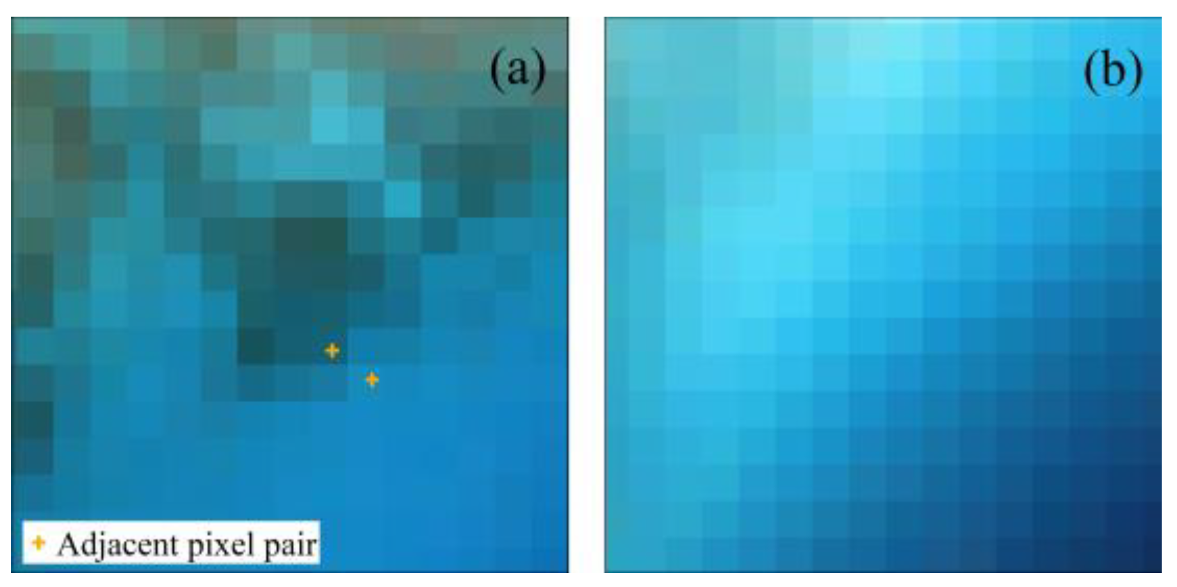
• Prioritize selecting adjacent pixel pairs that exhibit distinct boundaries between bright and dark pixels, as illustrated in Figure 11a. Avoid selecting adjacent pixel pairs within the same bottom type or in regions where the boundaries between different bottom types are blurred, as shown in Figure 11b.

• Ensure that the selected adjacent pixel pairs span different depth intervals. If a clearly defined waterline exists in the study area, select adjacent pixel pairs at varying distances from the waterline. In the absence of a waterline (e.g., in submerged reef environments), an isobath can be constructed based on the logarithmic ratio of blue to green band reflectance, expressed as $\frac{\mathrm{l}\mathrm{n}\left(1000R_{rs}\left(Blue\right)\right)}{\mathrm{l}\mathrm{n}\left(1000R_{rs}\left(Green\right)\right)}$. Pixels with equal values of this ratio are assumed to have the same depth. Adjacent pixel pairs should then be selected at varying distances from the same isobath.

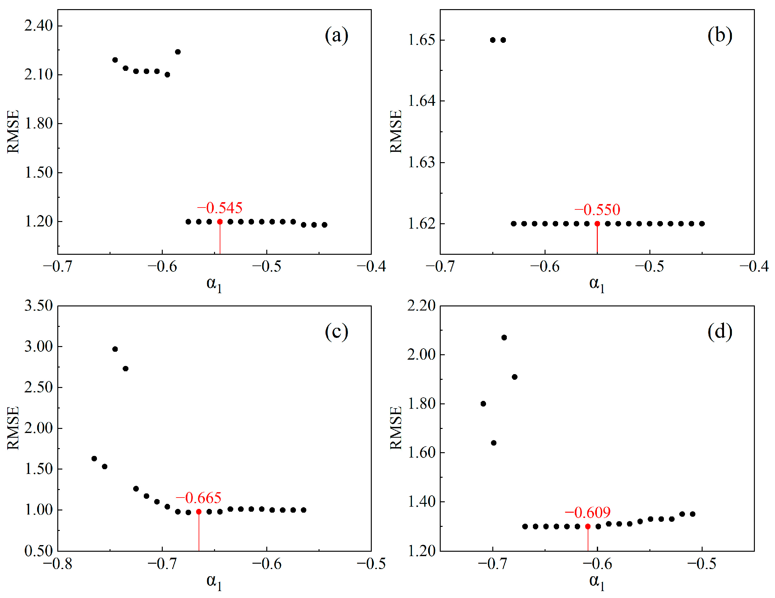
To verify the effectiveness of the optimal band-rotation coefficient unit vector estimated from adjacent pixel pairs, this study examined how variations in these unit vectors affect bathymetry retrieval accuracy. Using the estimated optimal band-rotation coefficient unit vectors as a baseline, the first component (${\alpha }_1$) was adjusted upward and downward by 0.1, with a step size of 0.01, to generate a series of perturbed unit vectors. The RMSE was then calculated for each vector. The results, shown in Figure 12, indicate that each subgraph exhibits a relatively flat RMSE distribution region, with values close to the global minimum. This suggests that within this region, multiple band-rotation coefficient unit vectors can achieve similarly optimal retrieval performance and can be considered equivalent solutions. Notably, the optimal band-rotation coefficient unit vectors estimated from adjacent pixel pairs in each study area represent such equivalent optimal solutions. This finding validates the reasonableness of the adjacent pixel pair selection criteria and the effectiveness of the estimated optimal unit vectors. Furthermore, within the variation range of ${\alpha }_1$, the RMSE changes for Buck Island, Yongxing Island, Kaneohe Bay, and Yongle Atoll were 1.06 m, 0.03 m, 2.00 m, and 0.77 m, respectively. These results indicate that the proposed model is sensitive to the optimal band-rotation coefficient unit vector in Buck Island, Kaneohe Bay, and Yongle Atoll, but less sensitive in Yongxing Island.

In conclusion, the proposed model is sensitive to the optimal band-rotation coefficient unit vector in most study areas. The estimated optimal unit vector, derived from adjacent pixel pairs, is valid and represents an optimal solution.

5.2. Impact of the Number of SIPs on Model Performance

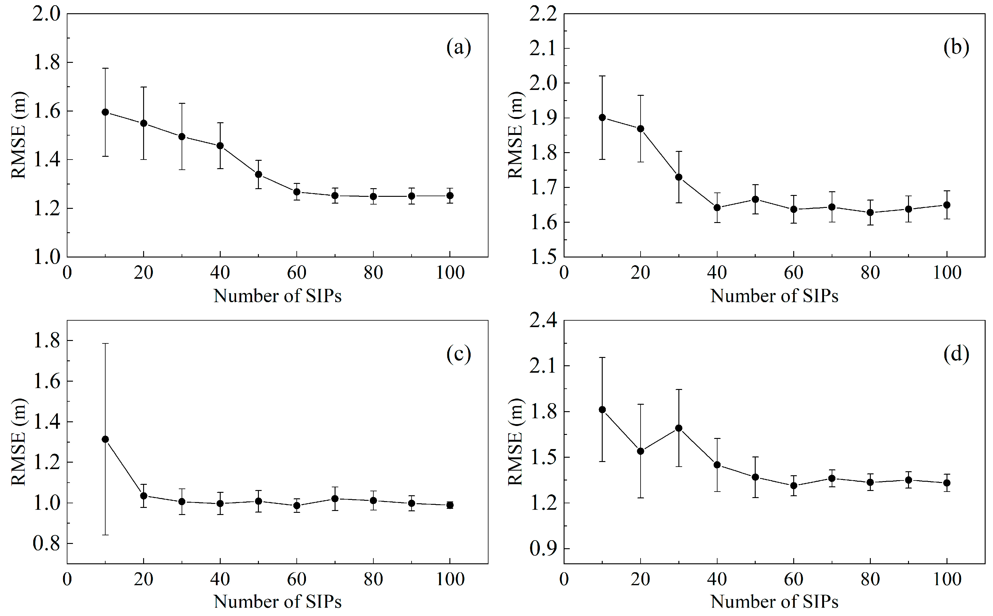
Figure 13 systematically illustrates the impact of the number of SIPs on model performance. The black circles represent the average RMSE values from ten independent experiments, with error bars indicating the standard deviation. As shown in Figure 13, RMSE decreases significantly across all study areas as the number of SIPs increases. When the number of SIPs approaches 70, 50, 30, and 60 for Buck Island, Yongxing Island, Kaneohe Bay, and Yongle Atoll, respectively, RMSE begins to stabilize, with fluctuations smaller than 0.05 m. Simultaneously, the standard deviation of repeated experiments in each study area also decreases significantly with an increasing number of SIPs and stabilizes at similar SIP counts, indicating enhanced repeatability of model outputs and a substantial reduction in uncertainty during parameter retrieval.

Overall, the 200 SIPs used in this study significantly exceed the minimum number required to achieve stable performance in each study area. This not only ensures that the proposed model delivers stable and reliable bathymetry retrieval in typical coral reef waters but also provides a valuable reference for SIP sampling strategies in marine environments with similar optical properties and underwater topographic features.

5.3. Impact of Atmospheric Correction on Retrieval Accuracy

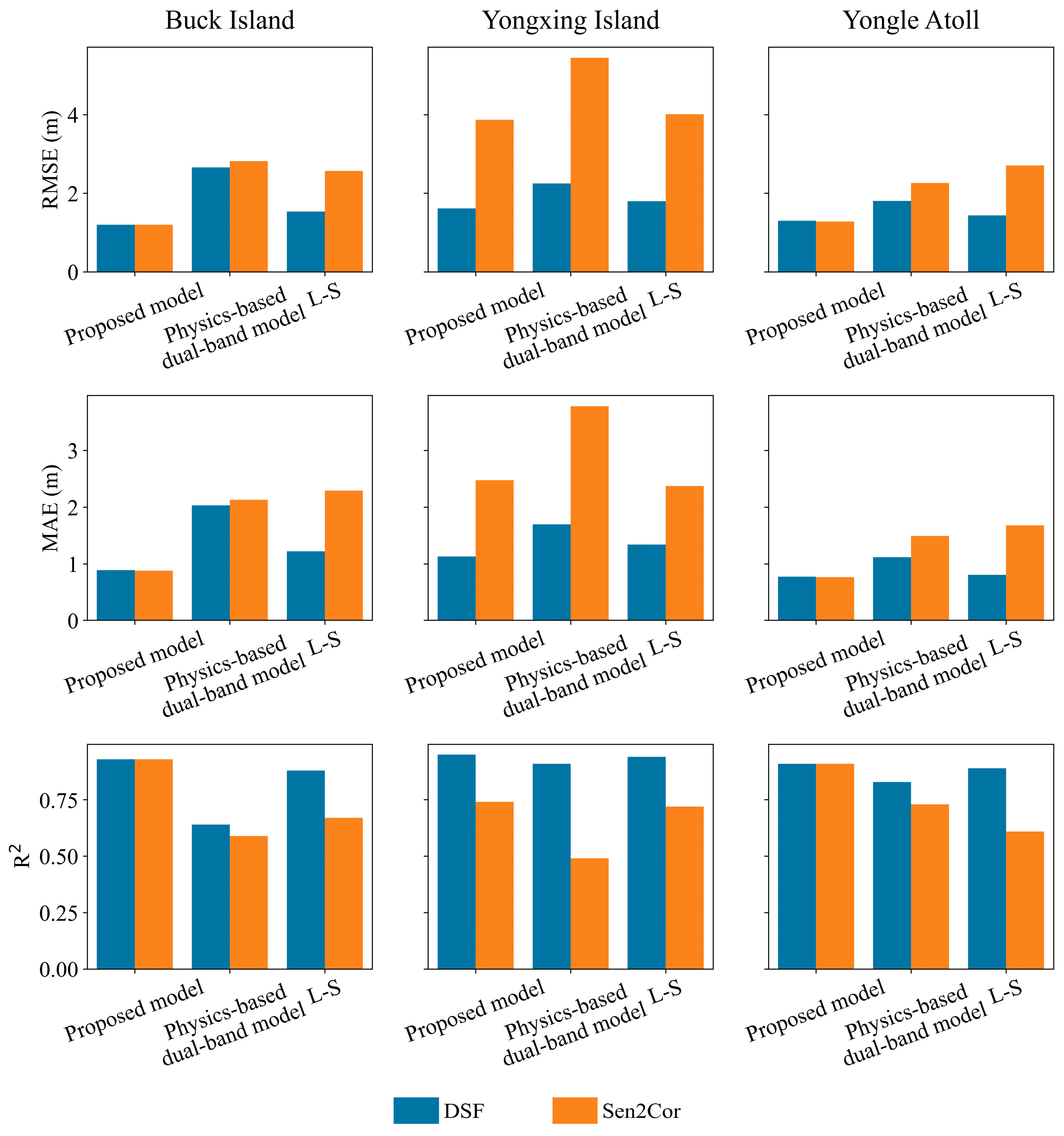
To evaluate the effectiveness of the proposed model on remote sensing images processed with different atmospheric correction algorithms, Sentinel-2 images from Buck Island, Yongxing Island, and Yongle Atoll were used to compare the bathymetry retrieval accuracy of the proposed model, the physics-based dual-band model, and the L-S model under two atmospheric correction methods: the DSF algorithm implemented in the ACOLITE v20250402.0 software, and the official Sen2Cor atmospheric correction algorithm provided by the European Space Agency for Sentinel-2 images. Previous studies have demonstrated that both the DSF and Sen2Cor algorithms are effective for shallow-water bathymetry retrieval in coral reef environments. It is important to note that the Gaofen-2 imagery from Kaneohe Bay was excluded from this comparison because validated sensor configurations for Gaofen-2 imagery are not available in either the DSF or Sen2Cor atmospheric correction frameworks. The comparison results using the DSF algorithm were detailed in Section 4.3. This study now focuses on presenting the comparison results using the Sen2Cor algorithm (see Figure 14). As shown in Figure 14, the proposed model demonstrates significant accuracy advantages over other models at Buck Island, Yongxing Island, and Yongle Atoll. The detailed comparison results are summarized below:

• Buck Island: The proposed model achieved an RMSE of 1.20 m, an MAE of 0.88 m, and an R² value of 0.93. Compared to the physics-based dual-band model, this represents reductions of 57% in RMSE and 59% in MAE, along with an increase of 0.34 in R². Relative to the L-S model, the improvements include a 53% lower RMSE, a 62% lower MAE, and a 0.26 higher R².
• Yongxing Island: The proposed model achieved an RMSE of 3.87 m, an MAE of 2.48 m, and an R² value of 0.74. These results correspond to a 29% reduction in RMSE and a 0.25 increase in R² compared to the physics-based dual-band model, as well as a 3% decrease in RMSE and a 0.02 increase in R² relative to the L-S model. Regarding MAE, the proposed model demonstrates a 34% reduction compared to the physics-based dual-band model (from 3.78 m to 2.48 m), but is approximately 5% higher than the L-S model (2.37 m).
• Yongle Atoll: The proposed model achieved an RMSE of 1.28 m, an MAE of 0.76 m, and an R² of 0.91. This corresponds to a 43% reduction in RMSE, a 49% reduction in MAE, and a 0.18 increase in R² compared to the physics-based dual-band model, as well as a 53% lower RMSE, a 55% lower MAE, and a 0.30 higher R² relative to the L-S model.

These results demonstrate that the proposed model maintains high bathymetry retrieval accuracy under the Sen2Cor atmospheric correction process and outperforms both the physics-based dual-band model and the L-S model, confirming its effectiveness on remote sensing images processed using this algorithm.

Figure 15 compares the performance of the DSF and Sen2Cor atmospheric correction algorithms in terms of bathymetry retrieval accuracy. For the proposed model, the DSF algorithm produced similar RMSE, MAE, and R² values in Buck Island and Yongle Atoll compared to the Sen2Cor algorithm. However, at Yongxing Island, the DSF algorithm achieved noticeably lower RMSE and MAE, as well as higher R², than Sen2Cor. For both the physics-based dual-band model and the L-S model, the DSF algorithm outperformed Sen2Cor across all study areas in terms of RMSE, MAE, and R². These results suggest that the DSF algorithm is more effective than Sen2Cor for bathymetry retrieval using physics-based approaches.

5.4. Limitations of the Proposed Model and Future Work

Physics-based approaches typically require high imaging conditions and superior image quality. As a physics-based method, the proposed model is no exception. In the future, it may be possible to stack multiple high-resolution multispectral images to synthesize a single high-quality image, thereby reducing the quality requirements for the proposed model. Additionally, the current model faces a time-consuming challenge when searching for the optimal combinations of P, G, and X. This search process often involves traversing numerous possible combinations, many of which are clearly unpromising. Future work could explore new search strategies to pre-screen and eliminate unpromising P, G, and X combinations, thereby skipping their computation and focusing computational resources on the more promising parameter sets. This approach would significantly enhance the model’s operational efficiency. Furthermore, the assumption that P, G, and X remain constant within a small area is a fundamental premise of the model; however, the applicability and limitations of this assumption have not been adequately discussed in this study. In future work, we will include a quantitative analysis of influencing factors, such as the spatial extent of the study area and the degree of variation in the optical properties of the water body.

6. Conclusions

This study addresses the challenge of reliably retrieving bathymetric maps from multispectral images containing only three visible light bands, a limitation inherent in existing physical methods. We propose a novel semi-analytical-empirical hybrid model. The core innovation of this model lies in integrating a semi-analytical model with the analytical expression of the dual-band model to quantify the relative water depth relationships among different pixels. This relationship is then used as a constraint to select the most physically valid water depth from multiple numerical solutions generated by the semi-analytical model. By using the derived depths from SIPs as a calibration dataset, the optimal bathymetric retrieval model for each study area is systematically selected, ultimately enabling the reliable generation of bathymetric maps for the entire region. The key conclusions drawn from the experimental results are as follows:

• The proposed model demonstrates exceptional accuracy and robustness across several typical coral reef environments, consistently producing stable bathymetric maps. In the four study areas—Buck Island, Yongxing Island, Kaneohe Bay, and Yongle Atoll—the model’s retrieval results (with RMSE values ranging from 0.98 to 1.62 m, MAE values from 0.73 to 1.13 m, and R² values between 0.91 and 0.95) significantly outperform existing mainstream bathymetry retrieval methods, such as the physics-based dual-band model and the L-S model, which do not rely on in situ depth measurements. Notably, the proposed model maintains excellent retrieval accuracy across all depth intervals, especially in deeper waters (>15 m), underscoring its robustness and broad applicability.
• Sensitivity analysis of the optimal band rotation coefficient unit vector reveals that, although the proposed model is sensitive to this vector in most regions, it can reliably obtain equivalent optimal solutions by adhering to a clear set of criteria for selecting adjacent pixel pairs. This ensures the method’s reproducibility. Furthermore, the analysis identifies the minimum number of SIPs required for stable model performance—ranging from 30 to 70—offering practical guidance for sampling strategies in future applications. Additionally, the proposed model maintains a significant accuracy advantage under both the ACOLITE DSF and Sen2Cor atmospheric correction algorithms, further demonstrating its robustness for real-world applications.

In summary, the proposed model demonstrates significant potential for application in regions lacking prior bathymetric information. However, it still faces limitations, including high image quality requirements and the need for improved computational efficiency. Future work could focus on enhancing its applicability and operational efficiency through image synthesis techniques and optimization of the parameter search strategy.

References

1. Yang, J.; Ma, Y.; Zheng, H.; Xu, N.; Zhu, K.; Wang, X.H.; Li, S. Derived Depths in Opaque Waters Using ICESat-2 Photon-Counting Lidar. Geophys. Res. Lett. 2022, 49, e2022GL100509. [Google Scholar] [CrossRef]
2. Su, H.; Liu, H.; Wang, L.; Filippi, A.M.; Heyman, W.D.; Beck, R.A. Geographically Adaptive Inversion Model for Improving Bathymetric Retrieval From Satellite Multispectral Imagery. IEEE Trans. Geosci. Remote Sens. 2014, 52, 465–476. [Google Scholar] [CrossRef]
3. Zhang, M.; Yang, F.; Wang, R.; Qi, C. High-Precision Water Depth Inversion in Nearshore Waters with SAR and Machine Learning. IEEE Geosci. Remote Sens. Lett. 2024, 21, 4003505. [Google Scholar] [CrossRef]
4. Li, N.; Tang, Q.; Chen, Y.; Dong, Z.; Li, J.; Fu, X. Satellite-derived bathymetry integrating spatial and spectral information of multispectral images. Appl. Opt. 2023, 62, 2017–2029. [Google Scholar] [CrossRef]
5. Wang, Y.; Zhou, X.; Li, C.; Chen, Y.; Yang, L. Bathymetry Model Based on Spectral and Spatial Multifeatures of Remote Sensing Image. IEEE Geosci. Remote Sens. Lett. 2020, 17, 37–41. [Google Scholar] [CrossRef]
6. Xu, N.; Ma, X.; Ma, Y.; Zhao, P.; Yang, J.; Wang, X.H. Deriving Highly Accurate Shallow Water Bathymetry From Sentinel-2 and ICESat-2 Datasets by a Multitemporal Stacking Method. IEEE J. Sel. Top. Appl. Earth Obs. Remote Sens. 2021, 14, 6677–6685. [Google Scholar] [CrossRef]
7. Chen, A.; Ma, Y.; Zhang, J. Partition satellite derived bathymetry for coral reefs based on spatial residual information. Int. J. Remote Sens. 2021, 42, 2807–2826. [Google Scholar] [CrossRef]
8. Cheng, J.; Chu, S.; Cheng, L. Advancing Shallow Water Bathymetry Estimation in Coral Reef Areas via Stacking Ensemble Machine Learning Approach. IEEE J. Sel. Top. Appl. Earth Obs. Remote Sens. 2025, 18, 12511–12530. [Google Scholar] [CrossRef]
9. Zhu, J.; Qin, J.; Yin, F.; Ren, Z.; Qi, J.; Zhang, J.; Wang, R. An APMLP Deep Learning Model for Bathymetry Retrieval Using Adjacent Pixels. IEEE J. Sel. Top. Appl. Earth Obs. Remote Sens. 2022, 15, 235–246. [Google Scholar] [CrossRef]
10. Lumban-Gaol, Y.; Ohori, K.A.; Peters, R. Extracting Coastal Water Depths from Multi-Temporal Sentinel-2 Images Using Convolutional Neural Networks. Mar. Geod. 2022, 45, 615–644. [Google Scholar] [CrossRef]
11. Duan, Z.; Cheng, L.; Mao, Q.; Song, Y.; Zhou, X.; Li, M.; Gong, J. MIWC: A multi-temporal image weighted composition method for satellite-derived bathymetry in shallow waters. ISPRS J. Photogramm. Remote Sens. 2024, 218, 430–445. [Google Scholar] [CrossRef]
12. Caballero, I.; Stumpf, R.P. Retrieval of nearshore bathymetry from Sentinel-2A and 2B satellites in South Florida coastal waters. Estuar. Coast. Shelf Sci. 2019, 226, 106277. [Google Scholar] [CrossRef]
13. Lowell, K.; Rzhanov, Y. Global and local magnitude and spatial pattern of uncertainty from geographically adaptive empirical and machine learning satellite-derived bathymetry models. GISci. Remote Sens. 2024, 61, 2297549. [Google Scholar] [CrossRef]
14. Casal, G.; Monteys, X.; Hedley, J.; Harris, P.; Cahalane, C.; McCarthy, T. Assessment of empirical algorithms for bathymetry extraction using Sentinel-2 data. Int. J. Remote Sens. 2018, 40, 2855–2879. [Google Scholar] [CrossRef]
15. Eugenio, F.; Marcello, J.; Mederos-Barrera, A.; Marques, F. High-Resolution Satellite Bathymetry Mapping: Regression and Machine Learning-Based Approaches. IEEE Trans. Geosci. Remote Sens. 2022, 60, 5407614. [Google Scholar] [CrossRef]
16. Hartmann, D.; Gravey, M.; Price, T.D.; Nijland, W.; de Jong, S.M. Surveying Nearshore Bathymetry Using Multispectral and Hyperspectral Satellite Imagery and Machine Learning. Remote Sens. 2025, 17, 291. [Google Scholar] [CrossRef]
17. Qi, J.; Zhang, D.; Ren, Z.; Cui, A.; Yin, F.; Qin, J.; Zhan, J.; Zhu, J. Determination of the Initial Value Ranges of Nonlinear Solutions for a Log Ratio Bathymetric Inversion Model and Bathymetry Retrieval. IEEE J. Sel. Top. Appl. Earth Obs. Remote Sens. 2021, 14, 10875–10888. [Google Scholar] [CrossRef]
18. Albright, A.; Glennie, C. Nearshore Bathymetry From Fusion of Sentinel-2 and ICESat-2 Observations. IEEE Geosci. Remote Sens. Lett. 2021, 18, 900–904. [Google Scholar] [CrossRef]
19. Huang, Y.; Yang, H.; Tang, S.; Liu, Y.; Liu, Y. An Appraisal of Atmospheric Correction and Inversion Algorithms for Mapping High-Resolution Bathymetry Over Coral Reef Waters. IEEE Trans. Geosci. Remote Sens. 2023, 61, 4204511. [Google Scholar] [CrossRef]
20. Zhang, X.; Chen, Y.; Le, Y.; Zhang, D.; Yan, Q.; Dong, Y.; Han, W.; Wang, L. Nearshore Bathymetry Based on ICESat-2 and Multispectral Images: Comparison Between Sentinel-2, Landsat-8, and Testing Gaofen-2. IEEE J. Sel. Top. Appl. Earth Obs. Remote Sens. 2022, 15, 2449–2462. [Google Scholar] [CrossRef]
21. Xu, C.; Ruan, X.; Shen, C.; Tao, Z.; Xu, X.; Zheng, J.; Wu, W. A subregional shallow water bathymetry derivation method for coral reef using ICESat-2 and Sentinel-2 combined with sediment information. Int. J. Appl. Earth Obs. Geoinf. 2025, 142, 104698. [Google Scholar] [CrossRef]
22. Jay, S.; Guillaume, M.; Minghelli, A.; Deville, Y.; Chami, M.; Lafrance, B.; Serfaty, V. Hyperspectral remote sensing of shallow waters: Considering environmental noise and bottom intra-class variability for modeling and inversion of water reflectance. Remote Sens. Environ. 2017, 200, 352–367. [Google Scholar] [CrossRef]
23. He, J.; Zhang, S.; Cui, X.; Feng, W. Remote sensing for shallow bathymetry: A systematic review. Earth-Sci. Rev. 2024, 258, 104957. [Google Scholar] [CrossRef]
24. Lee, Z.; Carder, K.L.; Mobley, C.D.; Steward, R.G.; Patch, J.S. Hyperspectral remote sensing for shallow waters. I. A semianalytical model. Appl. Opt. 1998, 37, 6329–6338. [Google Scholar] [CrossRef]
25. Lee, Z.; Carder, K.L.; Mobley, C.D.; Steward, R.G.; Patch, J.S. Hyperspectral remote sensing for shallow waters: 2. Deriving bottom depths and water properties by optimization. Appl. Opt. 1999, 38, 3831–3843. [Google Scholar] [CrossRef] [PubMed]
26. Cao, B.; Deng, R.; Xu, Y.; Cao, B.; Liu, Y.; Zhu, S. Practical Differences Between Photogrammetric Bathymetry and Physics-Based Bathymetry. IEEE Geosci. Remote Sens. Lett. 2022, 19, 8016705. [Google Scholar] [CrossRef]
27. Liu, Y.; Deng, R.; Li, J.; Qin, Y.; Xiong, L.; Chen, Q.; Liu, X. Multispectral Bathymetry via Linear Unmixing of the Benthic Reflectance. IEEE J. Sel. Top. Appl. Earth Obs. Remote Sens. 2018, 11, 4349–4363. [Google Scholar] [CrossRef]
28. Liu, Y.; Deng, R.; Qin, Y.; Cao, B.; Liang, Y.; Liu, Y.; Tian, J.; Wang, S. Rapid estimation of bathymetry from multispectral imagery without in situ bathymetry data. Appl. Opt. 2019, 58, 7538–7551. [Google Scholar] [CrossRef]
29. Liu, Y.; Zhao, J.; Deng, R.; Liang, Y.; Gao, Y.; Chen, Q.; Xiong, L.; Liu, Y.; Tang, Y.; Tang, D. A downscaled bathymetric mapping approach combining multitemporal Landsat-8 and high spatial resolution imagery: Demonstrations from clear to turbid waters. ISPRS J. Photogramm. Remote Sens. 2021, 180, 65–81. [Google Scholar] [CrossRef]
30. Lei, C.; Deng, R.; Liu, R.; Li, J.; Guo, Y.; Yang, J.; Hua, Z.; Zhang, R. Advancing Multispectral Image-Derived Physics-Based Bathymetry: Multi-Objective Evolutionary Computation for Shallow Water Depth Retrieval. IEEE J. Sel. Top. Appl. Earth Obs. Remote Sens. 2025, 18, 23858–23878. [Google Scholar] [CrossRef]
31. Li, J.; Knapp, D.E.; Schill, S.R.; Roelfsema, C.; Phinn, S.; Silman, M.; Mascaro, J.; Asner, G.P. Adaptive bathymetry estimation for shallow coastal waters using Planet Dove satellites. Remote Sens. Environ. 2019, 232, 111302. [Google Scholar] [CrossRef]
32. Xia, H.; Li, X.; Zhang, H.; Wang, J.; Lou, X.; Fan, K.; Shi, A.; Li, D. A Bathymetry Mapping Approach Combining Log-Ratio and Semianalytical Models Using Four-Band Multispectral Imagery Without Ground Data. IEEE Trans. Geosci. Remote Sens. 2020, 58, 2695–2709. [Google Scholar] [CrossRef]
33. Chen, B.; Yang, Y.; Xu, D.; Huang, E. A dual band algorithm for shallow water depth retrieval from high spatial resolution imagery with no ground truth. ISPRS J. Photogramm. Remote Sens. 2019, 151, 1–13. [Google Scholar] [CrossRef]
34. Xu, Y.; Cao, B.; Deng, R.; Cao, B.; Liu, H.; Li, J. Bathymetry over broad geographic areas using optical high-spatial-resolution satellite remote sensing without in-situ data. Int. J. Appl. Earth Obs. Geoinf. 2023, 119, 103308. [Google Scholar] [CrossRef]
35. McCarthy, M.J.; Otis, D.B.; Hughes, D.; Muller-Karger, F.E. Automated high-resolution satellite-derived coastal bathymetry mapping. Int. J. Appl. Earth Obs. Geoinf. 2022, 107, 102693. [Google Scholar] [CrossRef]
36. Zhu, W.; Ye, L.; Qiu, Z.; Luan, K.; He, N.; Wei, Z.; Yang, F.; Yue, Z.; Zhao, S.; Yang, F. Research of the Dual-Band Log-Linear Analysis Model Based on Physics for Bathymetry without In-Situ Depth Data in the South China Sea. Remote Sens. 2021, 13, 4331. [Google Scholar] [CrossRef]
37. Duan, Z.; Chu, S.; Cheng, L.; Ji, C.; Li, M.; Shen, W. Satellite-derived bathymetry using Landsat-8 and Sentinel-2A images: Assessment of atmospheric correction algorithms and depth derivation models in shallow waters. Opt. Express 2022, 30, 3238–3261. [Google Scholar] [CrossRef] [PubMed]
38. Zhu, W.; Huang, Y.; Cao, T.; Zhang, X.; Xie, Q.; Luan, K.; Shen, W.; Zou, Z. Satellite-Derived Bathymetry Combined with Sentinel-2 and ICESat-2 Datasets Using Deep Learning. IEEE J. Sel. Top. Appl. Earth Obs. Remote Sens. 2025, 18, 18376–18390. [Google Scholar] [CrossRef]
39. Yang, Q.; Chen, J.; Chen, B.; Tao, B. Evaluation and Improvement of No-Ground-Truth Dual Band Algorithm for Shallow Water Depth Retrieval: A Case Study of a Coastal Island. Remote Sens. 2022, 14, 6231. [Google Scholar] [CrossRef]
40. Legleiter, C.J.; Harrison, L.R. Remote Sensing of River Bathymetry: Evaluating a Range of Sensors, Platforms, and Algorithms on the Upper Sacramento River, California, USA. Water Resour. Res. 2019, 55, 2142–2169. [Google Scholar] [CrossRef]
41. Kerr, J.M.; Purkis, S. An algorithm for optically-deriving water depth from multispectral imagery in coral reef landscapes in the absence of ground-truth data. Remote Sens. Environ. 2018, 210, 307–324. [Google Scholar] [CrossRef]
Figure 1. Geographic distribution of the study areas. True-color composite images derived from multispectral remote sensing data for each study area. (a) Buck Island; (b) Yongxing Island; (c) Kaneohe Bay; (d) Yongle Atoll.
Remotesensing 17 03879 g001
Figure 2. Spatial distribution of in situ bathymetric data within the study area. (a) Buck Island; (b) Yongxing Island; (c) Kaneohe Bay; (d) Yongle Atoll.
Remotesensing 17 03879 g002
Figure 3. Example of identifying shallow-water regions through visual interpretation. Gray areas indicate masked land and environmental noise. The blue polygon represents the boundary of the shallow-water region. (a) True-color composite of the Sentinel-2 imagery. (b) False-color composite image generated by assigning Bands 3, 3, and 4 to the red, green, and blue channels, respectively. (c) False-color composite image generated by assigning Bands 2, 2, and 4 to the red, green, and blue channels, respectively.
Remotesensing 17 03879 g003
Figure 4. Water-leaving reflectance obtained from the preprocessed imagery. Gray areas indicate masked land and environmental noise. (a) Buck Island; (b) Yongxing Island; (c) Kaneohe Bay; (d) Yongle Atoll.
Remotesensing 17 03879 g004
Figure 5. Technical flowchart of the proposed model.
Remotesensing 17 03879 g005
Figure 6. Spatial distribution of sampled pixels. (a) Buck Island; (b) Yongxing Island; (c) Kaneohe Bay; (d) Yongle Atoll.
Remotesensing 17 03879 g006
Figure 7. Coefficients of determination (R2) of the 25 candidate bathymetry retrieval models on the calibration dataset for each study area.
Remotesensing 17 03879 g007
Figure 8. Bathymetric maps derived from the proposed model. (a) Buck Island; (b) Yongxing Island; (c) Kaneohe Bay; (d) Yongle Atoll.
Remotesensing 17 03879 g008
Figure 9. Scatter plots comparing derived bathymetry with in situ bathymetry for each study area. The red line represents the 1:1 line, indicating perfect agreement. Points above this line indicate overestimation of depth, while points below indicate underestimation.
Remotesensing 17 03879 g009
Figure 10. Comparison of retrieval errors of different models across different depth intervals.
Remotesensing 17 03879 g010
Figure 11. Example of adjacent pixel pair selection. (a) A region with distinct boundaries between bright and dark pixels; (b) a region with blurred pixel boundaries and a gradual transition.
Remotesensing 17 03879 g011
Figure 12. Impact of changes in optimal band-rotation coefficient unit vectors on bathymetry retrieval accuracy. Red circles represent the optimal band-rotation coefficient unit vectors estimated based on adjacent pixel pairs (only showing α 1 ). (a) Buck Island; (b) Yongxing Island; (c) Kaneohe Bay; (d) Yongle Atoll.
Remotesensing 17 03879 g012
Figure 13. Impact of the number of SIPs on model performance. (a) Buck Island; (b) Yongxing Island; (c) Kaneohe Bay; (d) Yongle Atoll.
Remotesensing 17 03879 g013
Figure 14. Scatter plot comparing the derived bathymetry with in situ measurements under the Sen2Cor atmospheric correction. The red line represents the 1:1 line, indicating perfect agreement. Points above this line indicate overestimation of depth, while points below indicate underestimation.
Remotesensing 17 03879 g014
Figure 15. Comparison of the DSF and Sen2Cor atmospheric correction algorithms on bathymetry retrieval accuracy.
Remotesensing 17 03879 g015