Article

Research on Forest Fire Smoke and Cloud Separation Method Based on Fisher Discriminant Analysis

College of Geo-Exploration Science & Technology, Jilin University, Changchun 130026, China
*
Author to whom correspondence should be addressed.
Remote Sens. 2025, 17(23), 3880; https://doi.org/10.3390/rs17233880
Submission received: 28 September 2025 / Revised: 14 November 2025 / Accepted: 26 November 2025 / Published: 29 November 2025

Highlights

What are the main findings?
  • The spectral responses of smoke and clouds vary significantly under different underlying surfaces. The study found that for dark underlying surfaces (vegetation and water), smoke and cloud spectra in the short-wave infrared show significant overall differences, while for bright underlying surfaces (soil), smoke and cloud spectra show the opposite trend from the near-infrared to the short-wave infrared.
  • Based on the screening of sensitive bands and the distribution patterns of smoke and clouds in spectral space, the Fisher discriminant analysis was used to construct the FSCRI model, which is suitable for vegetation, soil, and water underlying surfaces, achieving high discrimination accuracy with just a few bands.
What are the implications of the main findings?
  • The analysis of the spectral response differences in smoke and clouds under different underlying surfaces provides a theoretical basis for the construction of index models, thereby improving the accuracy of smoke and cloud discrimination.
  • The FSCRI model can effectively suppress the interference of clouds on smoke identification, provide strong technical support for early warning of forest fires, and improve the overall effectiveness of fire monitoring systems.

Abstract

In remote sensing monitoring of forest fires, smoke and clouds exhibit similar spectral characteristics in satellite imagery, which can easily lead to clouds being misjudged as smoke. This incorrect discrimination may result in missed detections or false alarms of fire points. The precise differentiation of smoke and clouds has become increasingly challenging, significantly limiting the ability to accurately identify fires in their early stages. Additionally, electromagnetic waves penetrating the smoke and clouds interact with the underlying surface, which interferes with the effective separation of smoke and clouds. In response to the aforementioned issues, this paper systematically studies the impact mechanism of different underlying surfaces on the spectral response of smoke and clouds. We constructed a dataset using sample collection and gradation methods. It contains smoke at varying concentrations and clouds of different thicknesses over three typical underlying surfaces: vegetation, soil, and water. Based on the analysis of spectral characteristics, analysis of variance (ANOVA) was applied to screen sensitive bands suitable for the separation of smoke and clouds. Furthermore, considering the distribution characteristics of smoke and cloud samples in spectral space, single-band threshold models, visible-band index (VBI) models, ratio index models, and Fisher smoke and cloud recognition index (FSCRI) models were developed for three typical underlying surfaces. The validation results demonstrate that the FSCRI models significantly outperform other models in terms of both robustness and accuracy. Their recognition accuracy rates for smoke and clouds in the underlying surfaces of vegetation, soil and water reached 95.5%, 93.5% and 99%, respectively. The proposed method effectively suppresses cloud interference to improve smoke and cloud separation. This capability enables more accurate early detection of forest fires and localization of their sources.

1. Introduction

Forest fires have a detrimental impact on the ecological environment, not only disrupting the ecosystem balance, but also causing substantial losses in human and material resources [1,2]. Therefore, early detection of forest fires is crucial for fire prevention and control. In the initial stages of a fire, the flames are typically weak, cover a small area, and are easily obscured by vegetation, making timely detection difficult for satellites, particularly those with medium or low resolution [3]. In contrast, smoke is the earliest and most significant remote sensing signal to appear during the forest fire, with a larger coverage area, making it the core source of information for earlier forest fire detection [4].
The extensive coverage, rich spectral information, and high spatial resolution of satellite imagery make the accurate detection of early fire smoke feasible [5,6]. As early as the 1970s, researchers began exploring the use of remote sensing satellites to detect and identify smoke for early forest fire monitoring [7]. Based on the physical relationship between smoke concentration and reflectance, Sun, Pan et al. [8] constructed a Mahalanobis distance index to characterize the spectral anomalies caused by smoke. Subsequently, they established a semi-physical and semi-empirical model of Mahalanobis distance–smoke concentration, achieving smoke identification and concentration inversion [9]. However, this method fails to effectively distinguish clouds from smoke due to the highly similar spectral properties. Cloud interference remains a core problem in smoke identification, seriously restricting the accuracy of early fire monitoring and becoming a widespread challenge in current satellite-based smoke detection research.
In the development of smoke and cloud differentiation methods, early studies primarily relied on visual interpretation and the analysis of morphological features for discrimination. Chung and Le [10] used NOAA satellite images and assigned different bands to the RGB channels to emphasize the visual differences between smoke and cloud. Nagatani et al. [11] used MODIS data and identified smoke and cloud through a false-color composite image created using the smoke reflectance index (SARI), short-wave infrared (SWIR), and the water index (WI). However, visual interpretation is highly dependent on manual analysis, which can result in significant errors and make it difficult to apply for the rapid processing of large-scale images. Miao et al. [12] developed an approach using edge detection technology to identify smoke based on its strip-like morphological features. Nevertheless, this method was only effective for strip smoke and clustered clouds.
To overcome the limitations of visual interpretation, researchers have gradually transitioned from relying on morphological features to automated multi-threshold identification algorithms based on spectral characteristics. Baum, Li, and Chrysoulakis [13,14,15] utilized the visible, near-infrared, and thermal infrared bands of the AVHRR satellite to classify and identify smoke, clouds, and underlying surface through a multi-threshold approach. However, limited spectral channels of the AVHRR satellite resulted in recognition accuracy that could not meet the requirements for high-precision monitoring. Jiang et al. [16] used radar satellite data to extract parameters such as horizontal reflectivity (ZH), differential reflectivity (ZDR), and correlation coefficient ( ρ H V ) of smoke clouds, and then set thresholds to identify smoke clouds. However, their threshold selection relied on experience, resulting in limited accuracy in smoke cloud identification. Xie et al. [17] developed a multi-threshold smoke plume detection method based on eight MODIS bands. Although this method gradually eliminated non-smoke pixels through thresholding, it still faced issues of missed detection and misclassification at cloud edges or in smoke-cloud mixed areas.
With the increasing abundance of visible light image data sources, researchers have begun using drone imagery and aerial photography datasets for model training. Javier et al. [18] used RGB images to effectively distinguish smoke and cloud regions based on the different fractal dimension distribution patterns of smoke and clouds in the images. However, in early fire detection, this method had low accuracy in identifying smoke and clouds due to the relatively faint smoke. Shang and Leon [19,20] used the You Only Look Once (YOLO) model, combining drone imagery with thermal infrared imaging and the fire weather index (FWI), to identify smoke and clouds. However, this model has limited ability to distinguish small-area smoke and cloud targets in the images.
In order to further improve the accuracy of smoke and cloud identification, researchers began to combine the differential characteristics of smoke and clouds in multiple spectral bands with machine learning methods. Wang et al. [21] utilized the difference in top-of-atmosphere (TOA) reflectance at 936 nm from MODIS, combined with the water absorption depth (WAD) of cloud and smoke, to effectively differentiate biomass burning smoke from clouds in marine environments using a decision tree method. However, this approach is limited to marine environments. Suo et al. [22] differentiated smoke and clouds by measuring the reflectance difference between the ultraviolet band (355 nm) and the red band (670 nm) using a decision tree classification method. However, the accuracy of this approach is dependent on a high-precision ultraviolet sensor, which restricts its applicability. Li et al. [23] integrated MODIS data with K-means clustering and Fisher discriminant analysis to achieve automated discrimination between smoke, cloud, water, and vegetation. However, the study did not consider the impact of seasonal variations on the model. Li et al. [24] further introduced seasonal training samples to develop a back-propagation neural network (BPNN) classification model, which achieved effective separation of smoke and clouds in spring, summer, and autumn. Nevertheless, the model showed limited effectiveness in detecting smoke and thin clouds.
To address the challenge of identifying smoke and thin clouds, recent research has shifted toward high-resolution satellite data. Wang and Wu [3,25] utilized Landsat 8 and Sentinel-2 satellite data, based on deep learning models such as U-Net and AttU-Net, and constructed models by combining multiple bands and extracting texture features of smoke and clouds, achieving the segmentation of smoke, clouds and other ground types. Wang et al. [26] utilized Sentinel-2 imagery and proposed a Summed Parameter of the Reflection Peak Difference (SPRPD) index based on the distinct reflectance peaks of smoke and cloud at 864 nm and 945 nm. This approach effectively distinguishes thin clouds from smoke when the underlying surface is vegetation. However, its performance in identifying smoke and clouds over other types of underlying surfaces remains to be validated. Current research methods predominantly focus on the influence of seasonal and regional variations on identification, while the potential interference from different underlying surfaces on the spectral characteristics of smoke and clouds has not been adequately addressed.
Both smoke and clouds are aerosol particles, and their spectral characteristics in satellite images represent a composite signal from both the aerosols and the underlying surface. Most existing studies have focused on the spectral analysis of high-concentration or high-thickness smoke clouds, ignoring the influence of the underlying surface on the spectral characteristics of smoke clouds. As a result, in medium- and low-resolution images, the missed detection rate of small areas of smoke clouds or light smoke and thin clouds is relatively high.
To address the aforementioned issues and further improve the accuracy of smoke and clouds recognition, this study focuses on examining the impact of different underlying surfaces on the spectral characteristics of smoke and clouds. Based on the absorption-scattering mechanisms of smoke and clouds, this study used Landsat 8/OLI images to construct a dataset of smoke at different concentrations and clouds of different thicknesses across underlying surfaces of vegetation, soil, and water. The spectral response characteristics of smoke clouds on different underlying surfaces and their distribution patterns in the two-dimensional spectral feature space were systematically analyzed. Analysis of variance (ANOVA) was applied to validate differences in spectral sensitivity across varying underlying surfaces. Using the single-band threshold method, the spectral index method, and Fisher discriminant analysis (FDA), smoke and cloud recognition models specifically for various underlying surfaces were systematically constructed. The accuracy, precision, recall, and F1 score of each model were calculated, and the models were subsequently applied to wildfire remote sensing image analysis, which supports the precise identification of wildfire smoke.
The article is organized as follows. In Section 2, the basic principles are introduced. In Section 3, the study area and data sources are described. In Section 4, the spectral characteristics of smoke and clouds and their sensitive bands are analyzed. In Section 5, smoke and cloud recognition models are developed, including single-band models, visible-band index (VBI) models, ratio index models, and Fisher smoke and cloud recognition index (FSCRI) models. In Section 6, application cases using satellite imagery are presented. In Section 7, the spectral mechanisms of smoke and clouds and the applicability of the models are discussed. In Section 8, the advantages of this study are summarized and future research directions are proposed.

2. Principles and Methods

2.1. Theoretical Basis of Remote Sensing Scattering for Smoke and Clouds

2.1.1. Smoke Aerosol

Forest fire smoke is essentially an aerosol, with its dispersed phase consisting of carbonaceous particles and water-soluble potassium (K+) generated from biomass burning, and air serving as the dispersant. Carbonaceous particles can account for up to 73% of the composition of smoke aerosols. These particles are primarily composed of two core components: organic carbon (OC) and elemental carbon (EC) [27,28].
From the perspective of particle physics characteristics, smoke aerosol particle size is primarily distributed in the range of 0.01–1 μm [29], which belongs to the category of typical fine particle aerosol. According to the physical parameters of smoke aerosol particles (including particle shape, particle size, concentration, particle size spectrum distribution and complex refractive index) [30,31,32,33], the radiative effect of such particles in the visible to near-infrared band is mainly Mie scattering—this scattering characteristic is one of the core physical foundations of smoke remote sensing detection.
Furthermore, the carbonaceous particles in smoke exhibit significant absorption of solar radiation. Across a broad spectrum from ultraviolet to thermal infrared band, these particles strongly absorb solar radiation, with the peak wavelengths for both absorption and scattering effects typically centered around 560 nm [34].

2.1.2. Cloud Aerosol

Clouds are visible aggregates in the atmosphere, formed by small water droplets or ice crystals resulting from the condensation of water vapor as it cools. Based on the temperature within the cloud and the phase of the cloud particles, clouds can be classified into three types: water clouds, composed of liquid water droplets; ice clouds, composed of ice crystal particles; and mixed-phase clouds, consisting of both liquid water droplets and ice crystals. When classified by altitude, clouds can be further divided into high, medium, and low clouds. High clouds are predominantly ice clouds, while medium and low clouds are mostly water clouds [35,36]. Both are easily confused with smoke in remote sensing images. Therefore, this paper focuses on the scattering–absorption characteristics of water clouds and ice clouds.
(1)
Water cloud remote sensing scattering mechanism
Water clouds are primarily found in the lower atmosphere where temperatures are relatively high. Due to the surface tension of water molecules, it is widely accepted that water clouds consist of spherical liquid water droplets. These droplets are the smallest cloud particles, with a typical radius of approximately 5 μm, and their overall size range is concentrated in the 2 to 25 μm range [37].
According to Mie scattering theory, the average extinction coefficient of water clouds in the visible to near-infrared band decreases as the effective radius of the cloud droplets increases. Within this spectral range, the absorption efficiency of water clouds is very low, meaning that the attenuation of electromagnetic wave energy is primarily due to scattering. However, as the wavelength increases, particularly in the short-wave infrared, absorption by water cloud particles becomes significantly stronger [38].
(2)
Ice cloud remote sensing scattering mechanism
Ice clouds primarily occur in the upper troposphere and lower stratosphere, and are composed of various nonspherical ice crystals. Existing ice cloud observation data indicate that the main forms of non-spherical ice crystals include solid columns, hollow columns, hexagonal plates, bullet rosettes, and aggregates [39,40,41]. Particle sizes span a wide range, from micrometers to centimeters, and typically follow a vertical distribution pattern, with smaller ice crystals at the cloud top and larger crystals at the cloud base.
From the perspective of scattering–absorption characteristics, ice clouds exhibit an albedo close to unity in the visible and near-infrared spectrum, indicating that scattering dominates the attenuation of electromagnetic energy. However, as the wavelength increases, the absorption effect of ice crystal particles becomes significantly stronger. At this point, the extinction coefficient of ice cloud particles decreases with an increase in the effective radius of the particles, while the albedo decreases as the absorption efficiency increases [42,43].

2.1.3. Comparison of Scattering–Absorption Mechanisms for Smoke and Clouds in Remote Sensing

Based on the analysis of the scattering–absorption characteristics of smoke and clouds (water clouds and ice clouds), their fundamental differences across spectral bands can be summarized as follows, providing a key theoretical basis for smoke and clouds identification in satellite images.
  • In the visible spectrum, clouds exhibit weaker absorption but stronger scattering compared to smoke particles. The reflectance of clouds is primarily determined by their optical thickness—both water and ice clouds show increased reflectance with greater optical thickness [44]. In contrast, smoke reflectance increases with aerosol concentration. Because the radius of cloud particles is much larger than that of smoke particles, their scattering ability is much stronger than that of smoke. Additionally, smoke particles exhibit a strong absorption effect in the visible light band. In the visible light range, for thick clouds, the particle radius is large, and the clouds are relatively thick. Incident electromagnetic waves are largely unable to penetrate the entire cloud layer, with most of the energy being scattered or reflected. As a result, the reflectivity of thick clouds is much higher than that of smoke. Within the visible light band, the reflectance variation patterns of smoke and clouds are similar, as both increase with an increase in their respective thickness or concentration. Consequently, the reflectance of thinner clouds and smoke becomes difficult to distinguish, leading to confusion between the two.
  • The short-wave infrared is a key spectral range for distinguishing smoke from clouds, with significant differences in their reflectance characteristics. Smoke particle radii are typically smaller than or close to the wavelength in this band, and their optical radiation is primarily Rayleigh and Mie scattering, resulting in a relatively weak overall scattering effect. Combined with strong absorption by components such as black carbon, smoke reflectance decreases significantly with increasing wavelength and remains generally low. Cloud particles are typically larger than the wavelength in this band, and radiation is primarily influenced by Mie scattering. Although their reflectance decreases with increasing wavelength, it can remain relatively high due to greater optical thickness. This effect is particularly pronounced in ice clouds, where multiple scattering by non-spherical particles helps maintain higher reflectance levels.
In summary, within the shortwave infrared band, the reflectivity of smoke should be lower than that of clouds. This key difference may be the crucial basis for distinguishing smoke and clouds in remote sensing images.

2.2. Research on Band Sensitivity Analysis Methods

2.2.1. Sensitive Bands for Smoke Concentration and Cloud Thickness

Analyzing the response differences in various bands to concentration/thickness changes under the same underlying surface is key to developing a high-precision smoke and cloud recognition model. This study employs analysis of variance and constructs a separability measurement index ( F ) to assess the ability of each band to distinguish smoke at different concentrations and clouds of different thicknesses.
ANOVA compares the within-group variation with the between-group variation to determine whether there are significant differences in the means of different groups [45]. In this study, the sum of squares between-group Q A reflects the differences between samples of different concentration/thickness grades, while the sum of squares within- group Q e represents the degree of variation within samples of the same grade. The F statistic is defined as:
F = Q A f A / Q e f e ~ F ( f A , f e )
Q A = i = 1 n j = 1 m ( x ¯ j x ¯ ) ,   Q e = i = 1 n j = 1 m ( x i j x ¯ j )
where m is the number of smoke/cloud concentration/thickness levels ( m = 5 ); n is the total number of smoke/cloud samples at each concentration/thickness level; x i j is the i th sample value at the j th concentration level, x ¯ j is the mean of the j th concentration/thickness smoke/cloud samples, and x ¯ is the total mean of the smoke/cloud samples; f A = m 1 is the degrees of freedom of Q A , and f e = m n m is the degrees of freedom of Q e .
Assuming that the means of the data in each group are equal (the null hypothesis H 0 indicates that this band is not sensitive to changes in smoke concentration/cloud thickness and is not a sensitive band), find the critical value F α ( f A , f e ) at the significance level α (in this paper, a significance level of α = 0.01 was chosen for analysis of variance to screen for sensitive bands. This choice is more stringent than the commonly used α = 0.1   or   0.05 , which can effectively reduce the risk of misclassifying non-sensitive bands as sensitive bands and improve the reliability of the selected bands and the robustness of the model). If F > F α ( f A , f e ) , then the null hypothesis is rejected at the significance level α , indicating that the band is sensitive to changes in smoke/cloud concentration/thickness and can be used as a sensitive band for smoke concentration/cloud thickness; otherwise, the null hypothesis is accepted.

2.2.2. Sensitive Bands for Smoke and Cloud Detection

Based on the concentration and thickness sensitivity analysis, in order to further distinguish between easily confused smoke and thin clouds, it is necessary to select feature bands that are sensitive to the differences in smoke and cloud categories. This method still uses the ANOVA and the separability measurement index F to determine whether a band has a significant ability to distinguish between smoke and cloud. In this process, the within-group sum of squares represents the internal variation in the same category (smoke or cloud) at a given concentration/thickness level, while the between-group sum of squares reflects the differences between smoke and cloud samples at that level. Continue to use Formula (1) to calculate the F -value and follow the above hypothesis testing process: if F > F α ( f A , f e ) , then it is considered that the band is sensitive to the smoke cloud category and is suitable for smoke and clouds separation.

2.3. Research on Smoke and Cloud Identification Methods

2.3.1. Threshold Method

A single band is selected as an indicator for smoke and cloud identification. Simply selecting a fixed threshold such as the median or mean is subjective and cannot ensure optimal classification performance. This study uses the receiver operating characteristic (ROC) curve and Youden’s index maximization method to determine the classification threshold. ROC is an effective tool for evaluating classification model accuracy. It helps us to comprehensively evaluate model performance at different thresholds and to determine the optimal classification threshold [46,47].
Suppose we have a set of samples with known true categories (smoke or cloud). We use a classification model to calculate the probability or score of each sample belonging to smoke. By setting a threshold, samples with scores above the threshold are classified as smoke and those below the threshold are classified as cloud. This yields the following classification results:
True Positive (TP), the number of samples whose true category is smoke and which are correctly classified as “smoke” by the model; False Positive (FP), the number of samples whose true category is “cloud” but is misclassified as “smoke” by the model; True Negative (TN), the number of samples whose true category is “cloud” and which are correctly classified as “cloud” by the model; False Negative (FN), the number of samples whose true category is “smoke” but is misclassified as “cloud” by the model.
Based on the above statistics, we can further define:
True Positive Rate (TPR), also known as sensitivity, indicates the proportion of samples that are correctly identified as “smoke”:
TPR = TP/(TP + FN)
A higher TPR indicates a stronger ability of the model to correctly identify smoke.
False Positive Rate (FPR) refers to the proportion of samples that are actually clouds but are incorrectly classified as “smoke”:
FPR = FP/(FP + TN)
A lower False Positive Rate (FPR) indicates fewer misclassifications of clouds as smoke.
Specificity (also called True Negative Rate, TNR) measures the proportion of actual cloud samples correctly identified:
TNR = TN/(TN + FP) =1 − FPR
The ROC curve is constructed by plotting the FPR on the horizontal axis and the TPR on the vertical axis, connecting the corresponding (FPR, TPR) points at different thresholds. The curve is formed by evaluating all possible thresholds. This study determines the optimal threshold by maximizing Youden’s index, defined as:
Youden’s Index = TPR + TNR − 1
Its geometric meaning is the vertical distance between a point on the ROC curve and the diagonal line. When Youden’s index reaches its maximum value, the corresponding threshold achieves the optimal balance between TPR and TNR. This point lies closest to the top-left corner of the ROC plot (FPR = 0, TPR = 1), indicating optimal discrimination between smoke and clouds at this threshold.

2.3.2. Spectral Index Method

Single spectral bands provide limited spectral information, and relying solely on the reflectance of a single band for smoke and cloud identification is highly limited and unreliable. We introduce a spectral index approach that combines multiple spectral bands sensitive to smoke and clouds into composite indices, with the goal of improving classification accuracy.
The spectral index method combines the reflectance of specific spectral bands in a mathematical manner, enabling dimensionality reduction while enhancing spectral differences between target objects such as smoke and clouds [48]. Based on the distribution patterns of smoke and cloud clusters in a two-dimensional spectral space and characteristic bands, we used operations such as summation and ratio to fuse multi-band reflectance information into a single index. On this basis, an optimal threshold was determined using the ROC curve and Youden’s index to establish a discrimination rule for effective classification of smoke and clouds.

2.3.3. Fisher Discriminant Analysis (FDA)

Each smoke and cloud sample contains reflectance information from seven bands. There is redundancy and overlap in this information, which hinders high-precision smoke and cloud identification. Spectral index methods can reduce redundancy by manually selecting bands and constructing an index, but they may also overcorrect and remove important information. Fisher Discriminant Analysis (FDA) is a classic linear classification method suitable for binary classification problems [49]. Its core goal is to find an optimal linear projection direction where samples of the same type (smoke samples or cloud samples) are clustered as closely as possible (minimizes the within-class scatter), while the centers of samples of different types (smoke samples and cloud samples) are as far apart as possible (maximizes the between-class scatter). The within-class scatter matrix S W and the between-class scatter matrix S B are defined as follows:
S W = q = 1 Q i = 1 Q q ( η i η ¯ q ) ( η i η ¯ q ) T
S B = q = 1 Q Q q ( η ¯ η ¯ q ) ( η ¯ η ¯ q ) T
where Q is the total number of smoke and cloud categories ( Q = 2 , representing smoke and cloud); Q q is the number of training samples in the q th category ( { q Z | 1 q 2 } , where q = 1 represents the number of smoke samples and q = 2 represents the number of cloud samples.); η ¯ is the mean vector of all smoke and cloud samples; η i represents the i th training sample vector; and η ¯ q represents the mean vector of the q th category training samples.
The FDA aims to maximize the ratio of between-class scatter to within-class scatter, which can be achieved by finding the eigenvalue:
S W 1 S B ω = λ
where the eigenvector ω corresponding to the largest eigenvalue λ represents the optimal projection direction. The linear discriminant function is defined as follows:
y = ω T x
where x is the input band vector, and y is the projected coordinate value. The coefficient ω associated with each band reflects its importance to the classification. Therefore, the coefficient can be used to select key bands and eliminate redundant information, thereby optimizing complex models and improving recognition accuracy.

3. Study Area and Data Sources

3.1. Overview of the Study Area

To systematically explore the spectral characteristics and identification methods of smoke and clouds over different underlying surfaces, this study selected regions with vegetation, soil, and water as the primary underlying surface types, including New South Wales and Victoria in Australia, and British Columbia in Canada. These regions are characterized by frequent forest fires, extensive smoke and cloud coverage, and diverse underlying surface types, which facilitate the acquisition of abundant and representative training samples.
(1)
New South Wales, Australia (28°~37°S, 141°~153°E)
The state is located on the southeastern coast of Australia and has a temperate oceanic climate, characterized by high summer temperatures that increase the likelihood of wildfires. The terrain is complex, with a variety of landforms, including mountains, grasslands, forests, water, and large areas of soil, distributed from the coast to the inland. On 8 October 2019, the northern part of the state experienced a major wildfire triggered by sustained high temperatures and lightning strikes. The fire lasted for 210 days, burning an area of 25,000 km2 [50,51]. This event provided samples of soil–smoke, soil–cloud, and vegetation–cloud.
(2)
Victoria, Australia (34°~39°S, 141°~150°E)
Located along the southeastern coast of Australia, the state has a coastline approximately 1800 km long. Its coastal climate is temperate maritime, while its inland climate is temperate continental. The southeastern area contains numerous lakes, and moist air masses from the ocean are transported inland, supplying ample moisture for cloud formation. These conditions facilitate the collection of a large number of water–cloud samples.
(3)
British Columbia, Canada (48°~60°N, 115°~140°W)
Bordering the Pacific Ocean to the west, the province has a Mediterranean climate, characterized by hot, dry summers and frequent forest fires. The province boasts a well-developed water system, with the Fraser River (1357 km) flowing through the western plains, creating a complex underlying surface of river–forest–soil. More than 50% of the province is covered by forests, primarily coniferous trees like pine and spruce—species with high oil content that are easy to trigger fire. Historically, the province has experienced numerous cross-regional forest fires, providing excellent conditions for selecting vegetation–smoke and water–smoke samples.

3.2. Data Source

3.2.1. Basis for Data Source Selection

To obtain samples of smoke and clouds over three types of underlying surfaces—vegetation, soil, and water—the selected satellite imagery must meet the following conditions: ① It must include three types of underlying surfaces; ② It must cover both smoke/cloud and their corresponding smoke/cloud-free underlying surface images; ③ The spatial resolution must be appropriate to clearly distinguish the details of smoke, clouds, and the underlying surface. Based on these requirements, this study selected Landsat-8 OLI/TIRS satellite imagery, which provides seven bands from visible to short-wave infrared (B1–B7, with central wavelengths of 0.440 μm, 0.482 μm, 0.562 μm, 0.655 μm, 0.865 μm, 1.609 μm, 2.201 μm).
Since a single Landsat-8 image cannot cover all three types of underlying surfaces simultaneously, this study adopts the strategy of region-specific targeted selection. (1) Vegetation: select British Columbia, Canada (smoke and smoke-free underlying surface samples, see Figure 1(a-1,a-2)) and Victoria, Australia (cloud and cloud-free underlying surface samples, see Figure 2(a-1,a-2)). (2) Soil: select a bushfire-scarred or farmland area in New South Wales, Australia (smoke and smoke-free underlying surface samples, see Figure 1(b-1,b-2), cloud and cloud-free underlying surface samples, see Figure 2(b-1,b-2)). (3) Water: select rivers and lakes around British Columbia, Canada (smoke and smoke-free underlying surface samples, see Figure 1(c-1,c-2)) and Victoria, Australia (cloud and cloud-free underlying surface samples, see Figure 2(c-1,c-2)).

3.2.2. Smoke and Cloud Sample Selection and Gradation Standards

To quantitatively analyze the spectral characteristics of smoke of different concentrations and clouds of different thicknesses on three underlying surfaces, a “visual interpretation + graded sampling” method was used to select samples. The specific process is as follows:
(1)
Sample gradation standards
Referring to existing remote sensing research [52] and combining the actual visual characteristics of smoke and clouds in the images, this study divides smoke into 5 levels according to concentration and clouds into 5 levels according to thickness (level 1 represents light smoke/thin clouds, and level 5 represents dense smoke/thick clouds). The classification is mainly based on the degree of obstruction of the underlying surface by smoke and clouds. A unified interpretation mark is established on the true color composite (R(4)G(3)B(2)) image (see Table 1 and Table 2), and interpretations are independently conducted by two professionals. For samples with inconsistent interpretation results, a consensus is reached through joint consultation to ensure consistency in the visual interpretation classification results.
Furthermore, in terms of physical mechanisms, and based on existing smoke concentration inversion models [9] the reflectance difference between the underlying surface and smoke regions within a single band can be attributed to the attenuation and scattering effects of smoke on electromagnetic radiation; similarly, the reflectance difference between the underlying surface and cloud regions is primarily caused by the cloud layer [53]. Since the reflectance of smoke and clouds usually increases with their concentration or thickness, the reflectance difference between underlying surface and smoke cloud samples can serve as an effective indicator for quantifying smoke concentration and cloud thickness.
To verify the reliability of the visually interpreted grading samples, a quantitative discrimination threshold was further constructed in this study. Based on the maximum reflectance difference between the densest smoke/thickest cloud area and the underlying surface, five intervals were divided using an equal-interval method, each corresponding to a discrimination threshold for different smoke concentrations/cloud thicknesses. During the sample validation phase, it was verified whether the reflectance difference between each smoke/cloud sample and its corresponding underlying surface fell within the threshold interval corresponding to its visual grading. All samples were verified individually to ensure the accuracy and consistency of the grading results.
(2)
Sampling method
For the three types of underlying surfaces—vegetation, soil, and water—we selected smoke samples across five concentration levels and cloud samples across five thickness levels. To minimize random errors, 500 pixels were randomly selected for each level, resulting in a sample set structured as 3 types of underlying surfaces × 10 types of targets × 500 pixels, totaling 15,000 valid samples. During the selection process, areas with a smaller range and a single type of underlying surface should be selected. Additionally, the edges of smoke or clouds should be avoided to ensure the purity of the sample and eliminate the influence of mixed pixels.

4. Spectral Characteristics and Band Sensitivity of Smoke and Clouds

To achieve accurate identification of smoke and clouds over different underlying surfaces, this study first extracts and analyzes sample spectra to identify the spectral differences between smoke and clouds, and then combines the analysis of variance to screen sensitive bands to provide a basis for subsequent discrimination models.

4.1. Spectral Characteristics of Smoke and Clouds

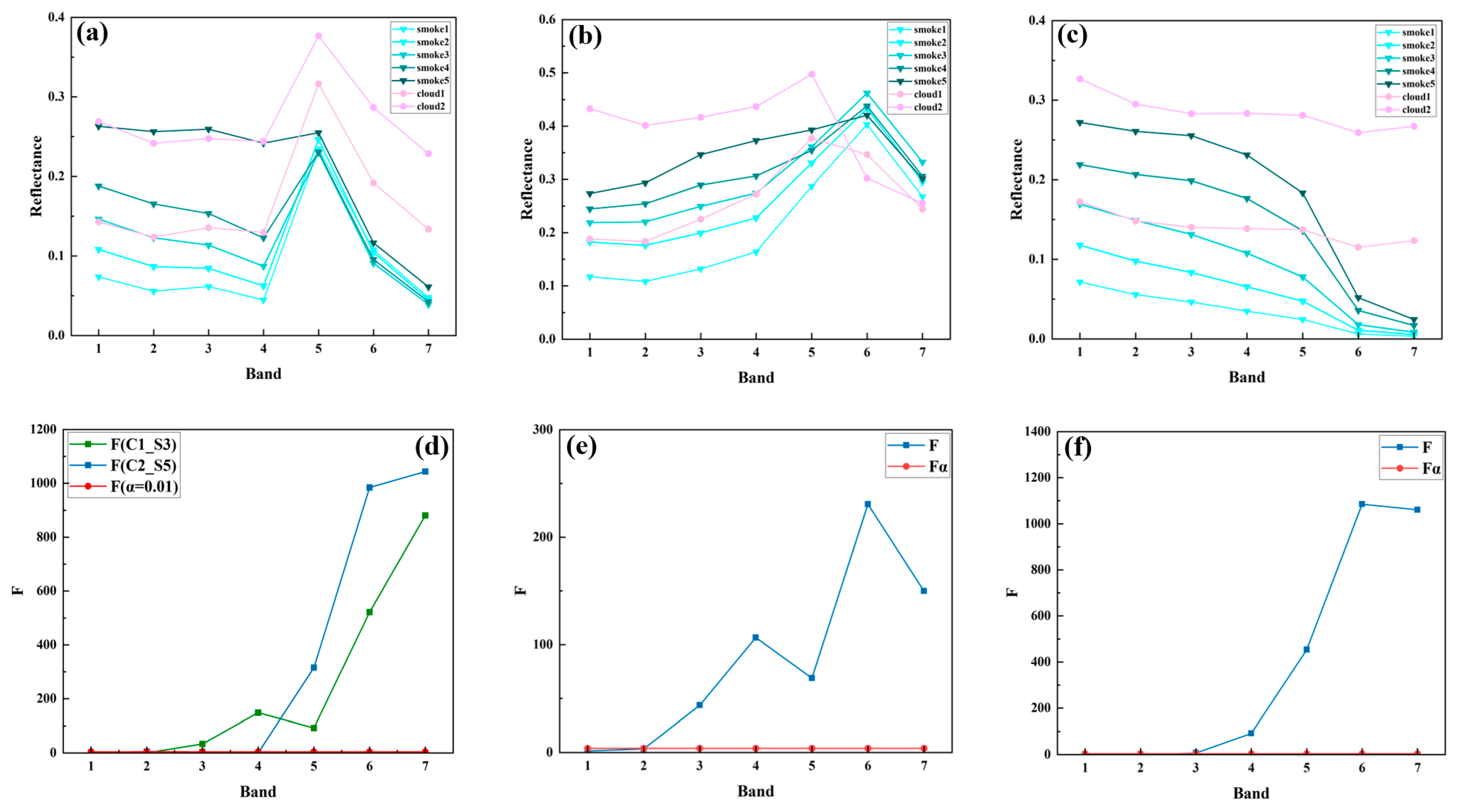
Figure 3 displays the average reflectance spectral curves of smoke at five concentration levels and clouds at five thickness levels against three types of underlying surfaces—vegetation (Figure 3a), soil (Figure 3b), and water (Figure 3c). Overall, except for some spectral overlap between low-thickness clouds and high-concentration smoke in certain bands, the reflectance of clouds is generally higher than that of smoke. Both smoke and clouds show similar spectral shapes in the visible to near-infrared range. In the visible bands (B1–B4), reflectance increases with higher concentration or thickness, consistent with Mie scattering theory. In the short-wave infrared bands (B6–B7), the reflectance significantly decreases, which is consistent with the theory of reduced scattering and enhanced absorption discussed above.
The spectral responses of smoke and clouds under different underlying surfaces exhibit significant differences. For the vegetation underlying surface (Figure 3a), smoke and thin clouds (levels 1–2) show an increasing reflectance trend in bands B4–B5 (red to near-infrared) and a decreasing trend in bands B5–B7 (shortwave infrared), with their overall spectral shapes resembling that of vegetation. For medium to thick clouds (levels 3–5), the reflectance increases with thickness in the visible to near-infrared range. For the soil underlying surface (Figure 3b), the reflectance of smoke increases in bands B5–B6, while clouds show a decreasing trend, with the decline becoming more pronounced as cloud thickness increases. Both smoke and clouds show a decrease in bands B6–B7, with smoke exhibiting a more significant reduction. In bands B1–B5, the reflectance of both smoke and clouds increases with concentration/thickness. For the water underlying surface (Figure 3c), reflectance generally decreases across bands B1–B7 for both smoke and clouds. Smoke declines most markedly in bands B5–B6, while medium to thick clouds (levels 3–5) exhibit strong reductions in bands B5–B7, with thick clouds (level 5) showing the greatest decrease in bands B5–B6.
These results confirm that smoke exhibits strong scattering in the visible bands, while its scattering effect weakens significantly in the near-infrared bands. Clouds generally have stronger scattering and absorption compared to smoke, with cloud reflectance ideally much higher than that of smoke. The spectral characteristics of smoke and clouds over different underlying surfaces are the result of the combined effects of their intrinsic scattering–absorption properties and the underlying surface spectra.

4.2. Overall Sensitivity Analysis of Smoke and Clouds over Different Underlying Surfaces

Through variance analysis, the F -values of seven bands for smoke with varying concentrations and clouds with different thicknesses were calculated. The F -values for each band were used to evaluate the sensitivity of the band to changes in smoke concentration and cloud thickness, with a higher F -value indicating greater sensitivity. The results (Figure 4) show that the F -values of all smoke cloud samples under the three underlying surfaces exceeded the critical value F ( α = 0.01 ) . For vegetation and soil underlying surfaces, the F -values of the bands B1–B4 (visible light) were generally higher than those of the bands B5–B7. For water underlying surfaces, the F -values of the bands B1–B5 were significantly higher than those of the bands B6–B7, indicating that the visible light bands are more sensitive to changes in smoke concentration and cloud thickness.
For the vegetation underlying surface (Figure 4a), the F -values for clouds in bands B5–B7 are significantly higher than those for smoke. In this underlying surface, the near-infrared to short-wave infrared bands are more sensitive to variations in cloud thickness but less sensitive to changes in smoke concentration, making them suitable for smoke and cloud discrimination. For the soil underlying surface (Figure 4b), the F -value for clouds in band 5 is significantly higher than that for smoke. In bands B6–B7, the F -values for both are similar but generally lower, indicating that band 5 is more sensitive to changes in cloud thickness and is thus an effective band for distinguishing smoke and clouds. For the water underlying surface (Figure 4c), bands B1–B5 maintain high sensitivity to both smoke and clouds. The F -values of smoke in bands B6–B7 are higher than that of clouds, indicating that the short-wave infrared band is more sensitive for identifying smoke and clouds.

4.3. Sensitivity Analysis of Smoke and Clouds over the Same Underlying Surface

For the combination of thin clouds (levels 1–2) and thick smoke (levels 3–5), which are most easily confused (Figure 3), targeted ANOVA was further conducted based on the overall sensitivity analysis to identify the characteristic bands that can effectively distinguish smoke and clouds.
Analysis of variance was conducted using the easily confused samples in the vegetation underlying surface, Cloud 1–Smoke 3 and Cloud 2–Smoke 5 (Figure 5a). The F -values for bands B5–B7 are significantly higher than those for the visible bands (Figure 5d), indicating that the near-infrared to short-wave infrared bands are the characteristic bands for distinguishing thin clouds from thick smoke in the vegetation underlying surface. For the soil underlying surface, ANOVA was performed using the easily confused samples: Cloud 1–Smoke 2 (Figure 5b). The F -values for bands B4–B7 are significantly higher than those for bands B1–B3 (Figure 5e), suggesting that these bands are suitable for distinguishing thick smoke and thin clouds in this underlying surface. For the water underlying surface, ANOVA was conducted using Clouds 1–Smoke 3 as easily confused samples (Figure 5c). The F -values of the bands B5–B7 were significantly higher than those of the visible bands (Figure 5f), making them key bands for distinguishing smoke and clouds from underlying surface.
The results of the band sensitivity analysis for smoke and clouds under different and the same underlying surface conditions show that the visible bands are more sensitive to changes in smoke concentration and cloud thickness, but have limited ability to distinguish between thick smoke and thin clouds, which are easily confused. In contrast, the near-infrared to short-wave infrared bands exhibit stronger discriminative capacity in such detailed scenarios. Therefore, for practical recognition, both types of bands should be combined to improve discrimination accuracy and robustness.

5. Construction and Verification of Smoke and Cloud Recognition Models

To effectively distinguish smoke and clouds over different underlying surfaces, this study constructed discrimination models for smoke and clouds using the single-band threshold method, the spectral index method, the ratio index method, and Fisher discriminant analysis. A comprehensive evaluation was then conducted from the perspectives of model separability and resistance to underlying surface interference.

5.1. Single-Band Threshold Model

Using the cross-validation method, 80% of all smoke and cloud samples from each underlying surface were randomly selected for modeling, while the remaining 20% were used for validation. By analyzing the spatial distribution and frequency distribution characteristics of smoke and clouds in bands B1–B7 across different underlying surfaces, a smoke and cloud recognition index was constructed. The discrimination thresholds for smoke and clouds in each band were determined using Youden’s index maximization method.
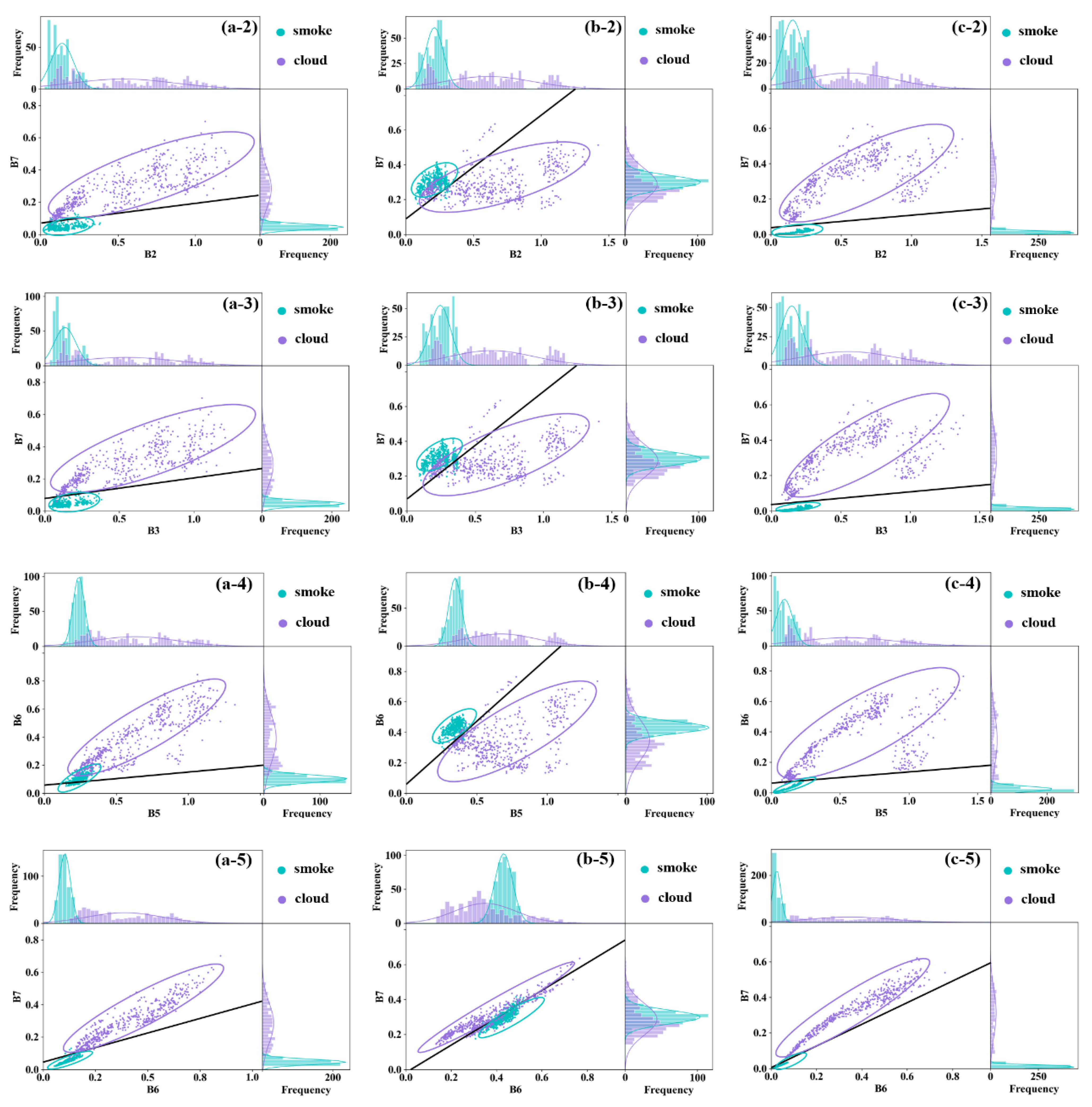
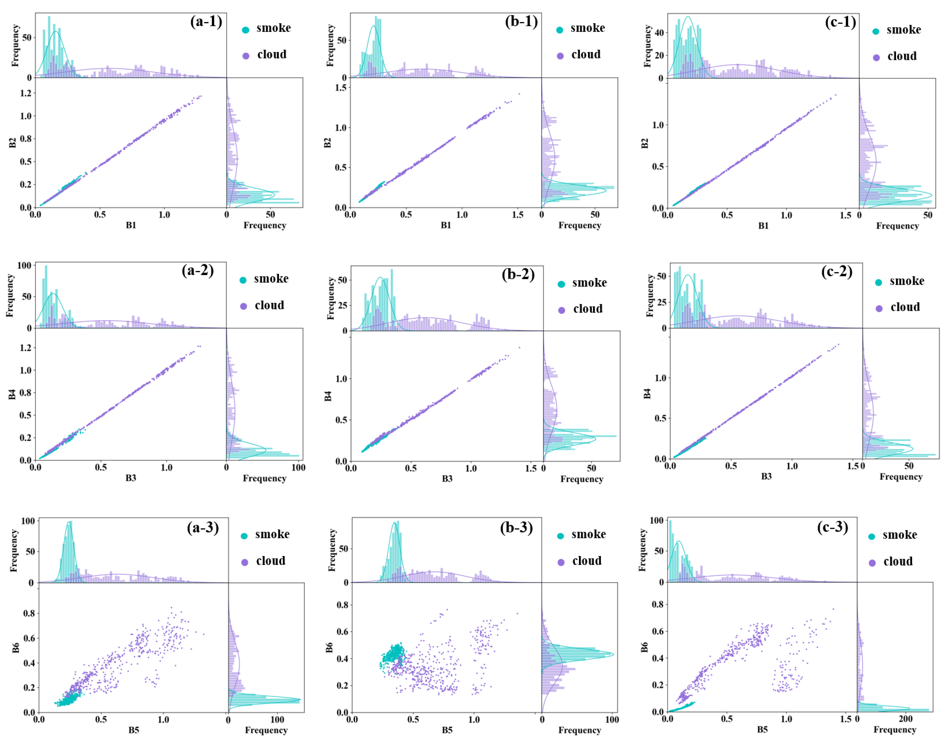
Figure 6 shows that in the spectral space composed of bands B1–B4, the distribution of smoke and cloud samples is concentrated and exhibits a linear trend. In the frequency histogram, the two point groups overlap significantly. However, in bands B5–B7, the separation between smoke and cloud points is noticeably improved, with reduced overlap and increasing separation as the wavelength increases. For the vegetation underlying surface, the recognition accuracy of bands B1–B4 is 6% lower than that of bands B5–B7 (Figure 11a). For the soil underlying surface, band B5 has the highest accuracy, exceeding the other bands by 7% (Figure 11b). For the water underlying surface, the accuracy of bands B1–B4 is approximately 10% lower than that of bands B5–B7 (Figure 11c). These results consistently demonstrate that the near-infrared bands (B5–B7) have superior discrimination capabilities compared to the visible bands, consistent with the conclusions of the band sensitivity analysis in Section 4. Notably, for the soil underlying surface, the point cluster overlap between bands B6–B7 increases, and discrimination accuracy decreases, which is also consistent with the previous results showing low sensitivity of these two bands in this underlying surface.

5.2. Visible-Band Index (VBI) Model

The visible-band index (VBI) is constructed based on the bands B1–B4, which are more sensitive to smoke concentration and cloud thickness:
VBI = B1 + B2 + B3 + B4
The VBI frequency distributions of smoke and cloud samples were statistically analyzed across the three underlying surfaces (Figure 7). The results indicate a high degree of overlap between thin clouds and smoke across all underlying surfaces. In the overall ANOVA across the three underlying surfaces, the VBI F -value was 737.57 ± 19.42, exceeding the significance level of α = 0.01   ( F α = 0.01 = 6.66 ) , with the discrimination accuracy measured at 85.07% ± 2.9%. However, obvious overlap remains between thick smoke and thin clouds. An additional ANOVA was conducted for this confusion combination. The F -values for the vegetation, soil, and water underlying surfaces were 4.97, 7.05, and 0.41, respectively ( F α = 0.01 = 6.69 ) , and the F -value for the water underlying surface was below the significance threshold. The results indicate that while VBI performs well overall, it has significant limitations in distinguishing thick smoke from thin clouds, consistent with the fact that visible light is sensitive to both smoke concentration and cloud thickness.

5.3. Ratio Index Model

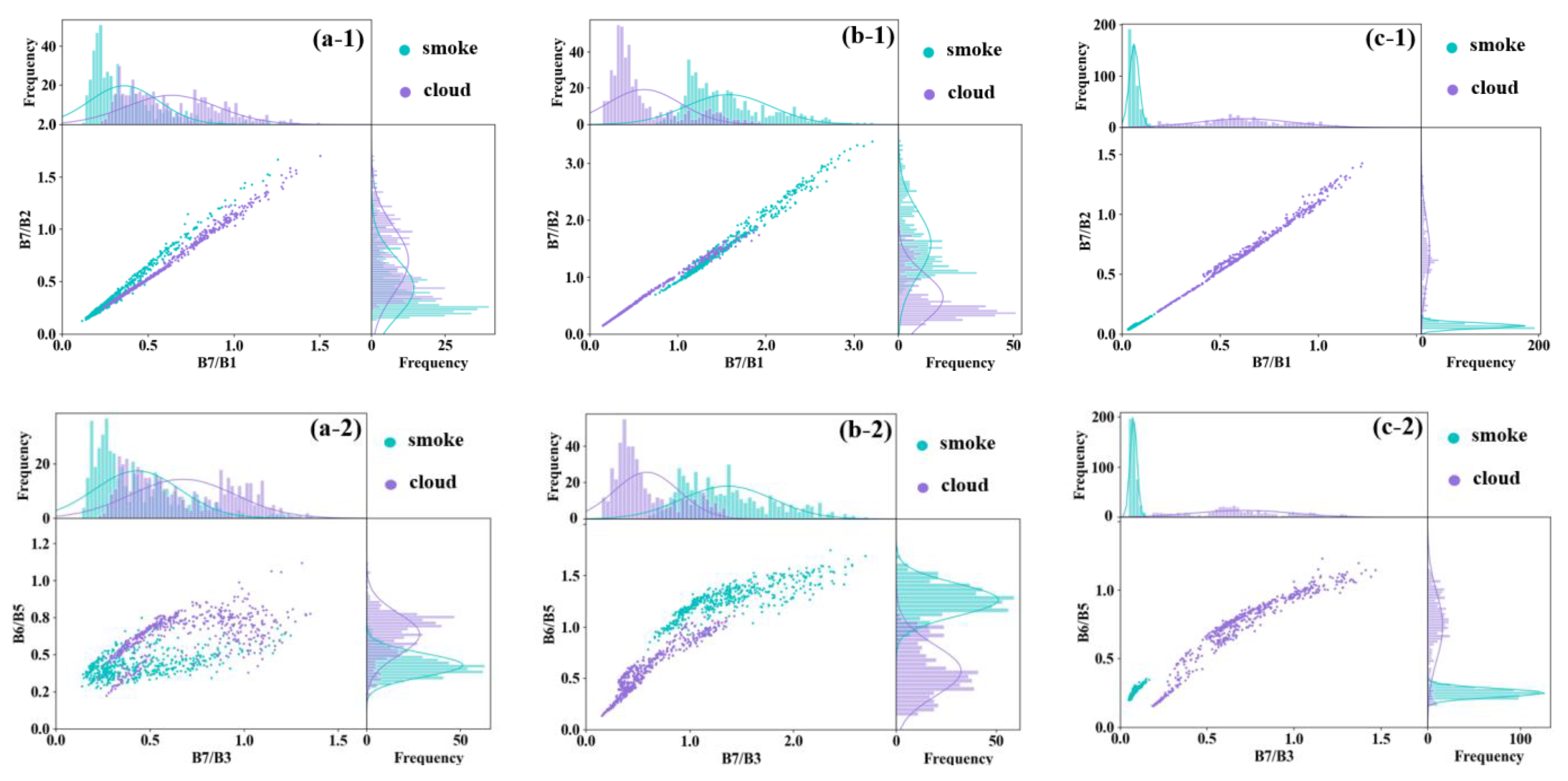
Given the high sensitivity of bands B6 and B7 in smoke and cloud identification, as well as the differences in the variation trends of smoke and clouds between bands B5–B6 under the soil underlying surface, this study developed five ratio indices—B7/B1, B7/B2, B7/B3, B7/B6, and B6/B5—to enhance the spectral differences between smoke and clouds. Figure 8 shows that within the two-dimensional index space formed by the B7/B1 and B7/B2 indices, the smoke and cloud point clusters exhibit a linear distribution. Among these, the highest degree of overlap between smoke and clouds occurs across vegetation underlying surface, while the best separation is achieved for water underlying surface. In the two-dimensional index space including B7/B6, the separation of smoke and cloud point clusters is most obvious for vegetation (Figure 8(a-2,a-3)) and water (Figure 8(c-2,c-3)) underlying surfaces. The F -value of B7/B6 in the vegetation underlying surface is 2397.37, exceeding the significance level of α = 0.01   ( F α = 0.01 = 6.66 ) , and the discrimination accuracy is 98.7% (Figure 11a). The F -value of B7/B6 in the water underlying surface is 5749.19, exceeding the significance level of α = 0.01   ( F α = 0.01 = 6.66 ) , and the discrimination accuracy is 100% (Figure 11c). The histogram overlap of B6/B5 in the soil underlying surface is the lowest (Figure 8(b-2,b-3)). The F -value of the B6/B5 index is 2805.36, exceeding the significance level of α = 0.01   ( F α = 0.01 = 6.66 ) , and the discrimination accuracy is 94.2% (Figure 11b).

5.4. Fisher Smoke and Cloud Recognition Index (FSCRI) Model

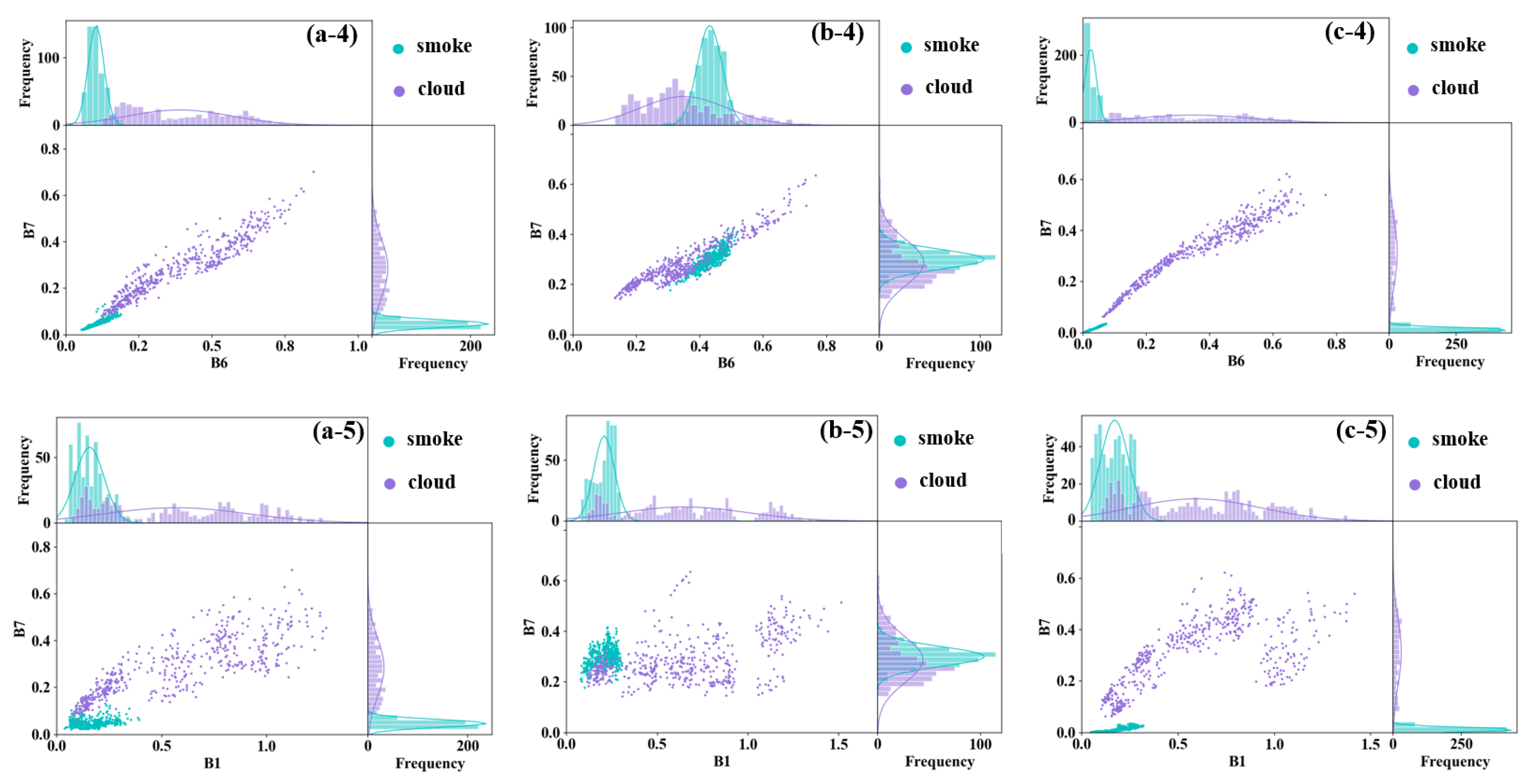
According to the results of variance analysis of easily confused smoke and thin clouds in different underlying surfaces (Figure 5), the F -values of B6 in the underlying surfaces of vegetation, soil and water are 423.21, 230.73 and 1085.15, respectively, and the F -values of B7 are 8105.49, 149.81 and 1061.05, respectively. The F -values of both bands are significantly higher than those of B1–B5. Therefore, B6 and B7 were selected to construct the Fisher smoke cloud recognition index (FSCRI). Given the high discrimination accuracy (94.2%) of the B5/B6 combination in the soil underlying surface, it was also incorporated into the recognition index. Based on the two-dimensional band scatter plot (Figure 9), in vegetation and water underlying surfaces, smoke and cloud point clusters are linearly separable in the spectral space formed by B7 with B1–B3, and B7 with B6. For the soil underlying surface, smoke and cloud point clusters exhibit high separability in the spectral space formed by B5 with B6. In summary, Fisher smoke and cloud recognition index (FSCRI) models are constructed for B7 with B1–B3, B5 with B6, as well as B7 with B6. The discriminant threshold (Table 3) was determined using the ROC curve by maximizing Youden’s index. A sample is distinguished as a cloud if FSCRI ≥ T, except for the FSCRIS-24567, FSCRIS-67, and FSCRIW-56 models, where FSCRI ≤ T distinguishes it as a cloud; otherwise, it is distinguished as smoke.
The results of the Fisher discriminant model show that the coefficients of each band reflect their contribution weights (Table 3). In the vegetation underlying surface, band 1, band 6, and band 7 have the largest coefficients; in the soil underlying surface, bands B5–B7 contribute significantly; and in the water underlying surface, band 2 and band 7 predominate. These results are consistent with the bands selected based on the characteristic bands and two-dimensional scatter plots, thereby validating the effectiveness of the characteristic band screening.
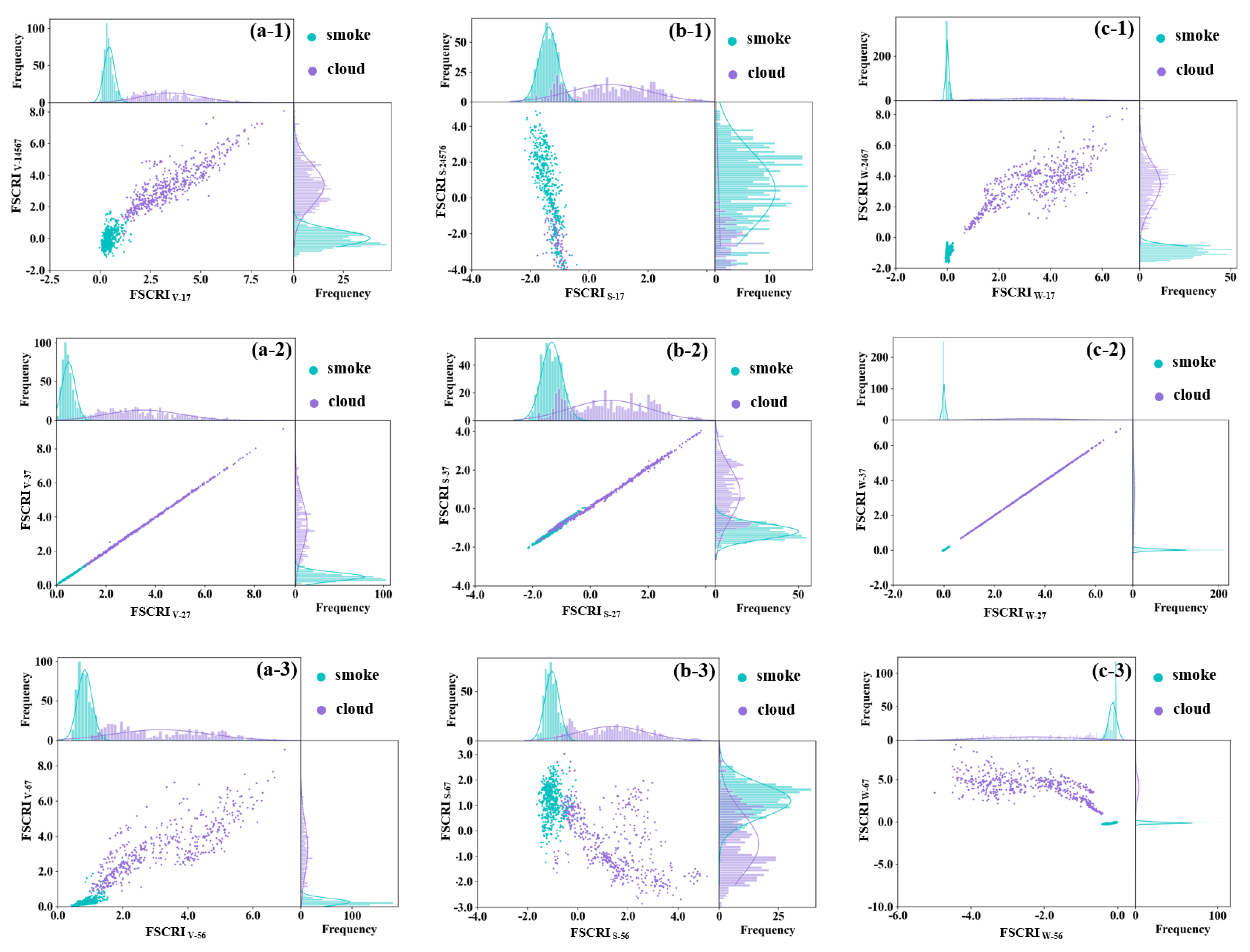
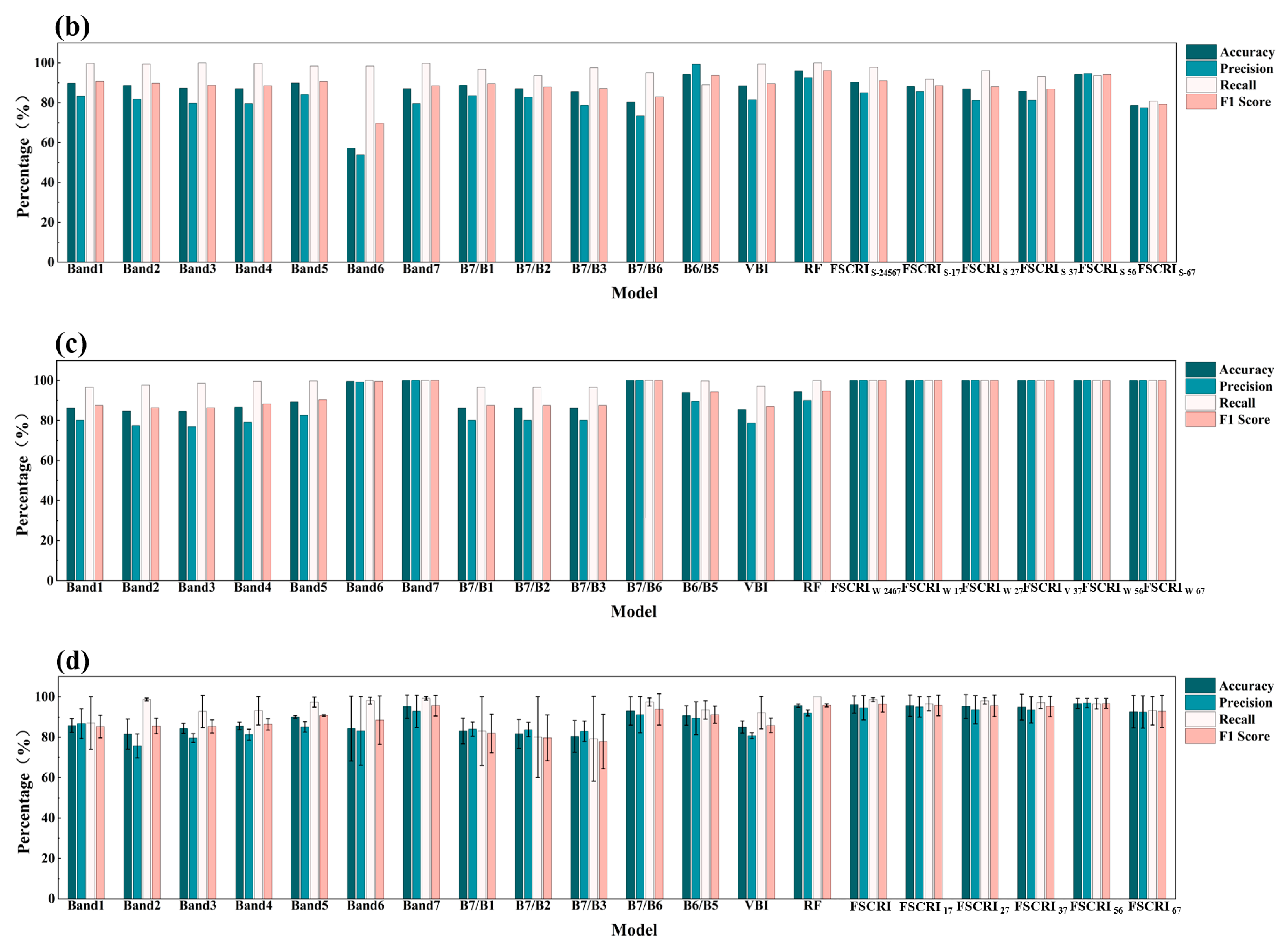
As shown in Figure 10, the FSCRI histograms demonstrate minimal overlap and clear separation between smoke and cloud clusters across three underlying surfaces. An exception occurs in the soil underlying surface, where FSCRIS-67 exhibits partial overlap (Figure 10(b-3)). The accuracy, precision, recall, and F1 score of each model and existing random forest (RF) classification method were calculated using 20% validation samples (Figure 11). Overall, the FSCRI discriminant method effectively distinguishes between smoke and clouds and outperforms both the single-band threshold method and the index method under various underlying surface conditions. Among them, FSCRIX-56 (X can be V, S, or W) achieves a relatively high recognition accuracy in all underlying surfaces, with a small fluctuation range of accuracy, demonstrating higher model robustness. As shown in Figure 11d, the total accuracy of this model under three underlying surfaces is 96.77% ± 2.41%, and the F1 score is 0.967 ± 0.024, which is the highest F1 score among all FSCRI. The random forest classification method also achieved good recognition accuracy in smoke and cloud recognition (Figure 11). The overall accuracy of this method under the three underlying surfaces was 95.67% ± 0.85%, and the F1 score was 0.958 ± 0.01. The overall accuracy was slightly lower than the best-performing FSCRI. For the vegetation underlying surface, the FSCRIV-67 index exhibited optimal performance across all metrics. For the soil underlying surface, FSCRIS-56 demonstrated the best discriminant capability. All FSCRI exhibited excellent recognition ability in the water underlying surface. Notably, the FSCRI constructed using all available bands did not significantly outperform other FSCRI combinations in any metric, further underscoring the importance of characteristic band selection for enhancing both model efficiency and discriminative power.
Figure 9. The two-dimensional band scatter plot and frequency distribution histogram composed of the bands used to construct the Fisher smoke and cloud recognition model. (a-1a-5) Vegetation; (b-1b-5) Soil; (c-1c-5) Water. The scatter plot has x and y axes representing the bands, showing the relationship between smoke and cloud point clusters in the two-dimensional spectral space. The histogram at the top shows the frequency distribution of smoke and cloud samples corresponding to the x-axis, along with the normal distribution curve. The histogram on the right shows the frequency distribution of smoke and cloud samples corresponding to the y-axis, also with the normal distribution curve. The black line in the figure represents the Fisher smoke and cloud recognition model constructed from this band combination. The purple ellipse encloses cloud samples, while the blue ellipse encloses smoke samples.
Remotesensing 17 03880 g009aRemotesensing 17 03880 g009b
Figure 10. Two-dimensional index scatter plots and frequency distribution histograms of smoke and cloud samples based on the FSCRI under different underlying surfaces. (a-1a-3) Vegetation; (b-1b-3) Soil; (c-1c-3) Water. The scatter plot has x and y axes representing the FSCRI, showing the relationship between smoke and cloud point clusters in the two-dimensional index space. The histogram at the top shows the frequency distribution of smoke and cloud samples corresponding to the x-axis, along with the normal distribution curve. The histogram on the right shows the frequency distribution of smoke and cloud samples corresponding to the y-axis, also with the normal distribution curve.
Remotesensing 17 03880 g010
Figure 11. The accuracy index histograms of each model and the random forest model (RF). (a) Vegetation; (b) Soil; (c) Water; (d) The overall accuracy index of each model in three underlying surfaces. Accuracy = (TP + TN)/(TP + FP + TN + FN), which reflects the proportion of smoke cloud samples that the model correctly predicted out of the total sample. Precision = TP/(TP + FP), which reflects the probability that the samples predicted as smoke by the model are actually smoke. Recall = TP/(TP + FN) denotes the proportion of samples that are actually smoke and are correctly identified as smoke, which represents the model’s ability to recognize “smoke samples”. F1 = (2 × Precision × Recall)/(Precision + Recall). The F1 score reconciles precision and recall to provide a more comprehensive evaluation result.
Remotesensing 17 03880 g011aRemotesensing 17 03880 g011b

6. Case Study: Verification of Forest Fire Smoke Identification and Cloud Separation

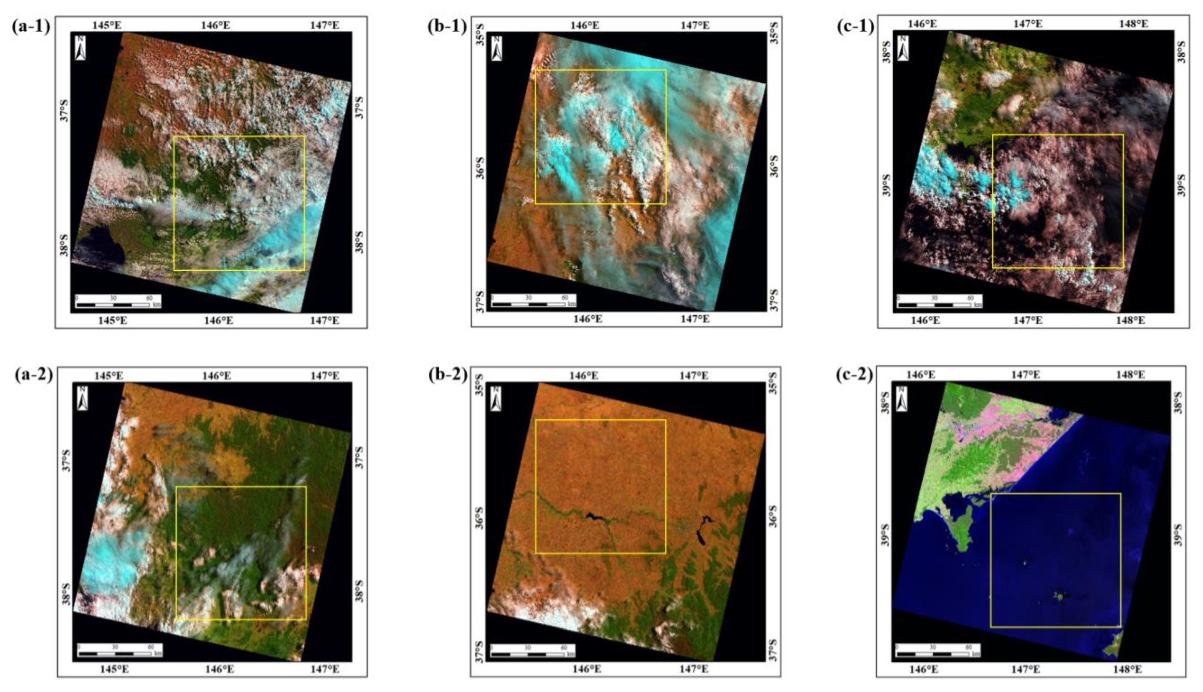
To validate the applicability of the proposed method, samples that were not involved in the initial modeling were selected for testing. In November 2019, a large-scale forest fire occurred in the mountainous region near New South Wales, Australia (35°S, 150°E), affecting an area of over 25,000 km2. For validation, a satellite image of the area taken on 31 December 2019, was used (Figure 12). The image covers various typical underlying surfaces, including vegetation, soil, and water. Moreover, the image was captured under weather conditions, providing an ideal scenario for testing the smoke and cloud detection algorithm.
First, the smoke detection method based on Mahalanobis distance (MD) proposed by Sun et al. (2023) [9] was applied for smoke target extraction. Subsequently, using the FSCRI discrimination index developed in this study, the vegetation underlying surface index FSCRIV-67, soil underlying surface index FSCRIS-56, and water underlying surface index FSCRIW-67 were applied to the separation of smoke and cloud pixels in different underlying surfaces. Meanwhile, the random forest (RF) method is utilized to separate the smoke and clouds on different underlying surfaces.
The results (Figure 12(a-3–d-3)) showed that although MD method was able to identify smoke in the smoke-cloud mixed regions, it also misclassified most clouds as smoke, resulting in a high false detection rate. The discriminative performance of FSCRI is significantly superior to that of the Mahalanobis distance (MD) method. This can be attributed to the inherent mechanisms of the two methods. The MD method is fundamentally an anomaly detection algorithm, which calculates the generalized distance between the target spectrum and the underlying surface spectrum. In this study, both smoke and clouds exhibit significant spectral anomalies relative to the underlying surface, such as vegetation and water, allowing the MD method to effectively separate smoke and clouds as a whole from the underlying surface. However, due to the highly similar spectral characteristics of smoke and clouds in specific bands, the MD method struggles to effectively distinguish between them within the “anomaly set” they form.
In contrast, the FSCRI method proposed in this study does not rely on the measurement of a single outlier but on the distinct physical mechanisms of smoke and clouds (such as aerosol particle size, complex refractive index) for systematic modeling. Fisher discriminant analysis captures the subtle spectral differences between smoke and clouds by seeking the optimal projection direction, maximizing the variance between classes (smoke and cloud), and minimizing the variance within classes, thereby achieving the separation of smoke and clouds. As a result, the FSCRI method can identify smoke and clouds more accurately and can be considered an improvement over the MD smoke recognition method. The Mahalanobis distance can be used to remove underlying surface pixels without smoke or clouds during the smoke and cloud separation process.
Figure 11 demonstrates that both random forest and FSCRI effectively distinguish between smoke and clouds compared to the Mahalanobis distance, with significantly fewer misclassifications. However, the FSCRI model proposed in this paper is simpler than the random forest classification method, achieving high recognition accuracy with only a few bands, significantly reducing computational cost, while still meeting the experimental requirements.
For the FSCRI identification results, random samples of smoke and cloud pixels were selected equally from pure vegetation, soil, and water areas, and accuracy validation was conducted using a confusion matrix. The results (Table 4) indicate that the overall accuracy of smoke and cloud discrimination reached 96% ± 2.27%. The misclassification rate for smoke pixels was relatively low, at 1.33% ± 0.94%, while the error rate for cloud pixels was somewhat higher, at 6.67% ± 3.68%. Due to the lower reflectance of water, which preserved the spectral differences between smoke and clouds more effectively, the detection accuracy in this underlying surface was the highest, surpassing both vegetation and soil underlying surfaces.
The FSCRI method achieved high recognition accuracy using only a few spectral bands across different underlying surfaces. The accuracy for water was 99%, for soil it was 95.5%, and for vegetation it was 93.5%. The misclassification rate for smoke pixels across all underlying surfaces was below 2%, indicating that the method is highly applicable and stable across various environments, fulfilling the requirements for practical operational applications.

7. Discussion

7.1. Correlation Analysis of Smoke and Cloud Scattering–Absorption Mechanisms with Multi-Spectral Responses

Based on the aforementioned fundamental physical mechanisms of scattering and absorption, the differences in spectral behavior between smoke and clouds, from the visible to the short-wave infrared bands, can primarily be attributed to disparities in their optical processes, which are governed by particle properties, such as radius and complex refractive index. The spectral response patterns observed in this study across various underlying surfaces were highly consistent with this theoretical framework.
In the visible bands (B1–B4), both smoke and cloud reflectance increase with concentration or thickness (Figure 3), and their spectral curves are similar. Thicker clouds have significantly higher scattering capacity than smoke, resulting in much greater reflectance in the visible bands and thus higher separability between the two. In contrast, thin clouds and smoke exhibit relatively similar reflectance levels, making them more prone to confusion. This phenomenon is closely related to the dominant role of Mie scattering in this band. Although there are differences in particle size, the overall scattering behavior of both is similar in this range, and the contribution of absorption is negligible. Therefore, in the spectral curve of smoke and clouds, the reflectance difference between smoke and thin clouds in the visible light range is minimal, making it difficult to achieve a stable distinction between the two using only visible light.
The near-infrared and short-wave infrared bands (B5–B7) exhibit significant spectral separation (Figure 5), making this region essential for distinguishing between smoke and clouds. On the one hand, the fine carbonaceous particles predominant in smoke exhibit strong absorption, resulting in overall low reflectance, which further decreases with increasing wavelength (Figure 3). On the other hand, cloud particles—especially ice clouds—have relatively large particle sizes, where Mie scattering remains dominant. Multiple scattering also occurs, allowing clouds to maintain high reflectance levels in the short-wave infrared (Figure 3). The experimental results are highly consistent with the theoretical results. As shown in Figure 3a,c, the reflectance of clouds in the short-wave infrared (B6–B7) is significantly higher than that of smoke in dark underlying surfaces (vegetation and water), which aligns with the theoretical derivation. In bright underlying surfaces (soil), smoke is strongly affected by the underlying surface, causing a significant increase in reflectance in the B6 band. Smoke and clouds exhibit distinct spectral response trends in the B5–B6 range (Figure 3b), providing a strong theoretical foundation for the recognition of smoke and clouds under bright underlying surface conditions. This further validates the physical superiority of the near-infrared and short-wave infrared bands (B5–B7) for recognition and offers a theoretical basis for constructing a robust discriminative model.

7.2. Impact of Underlying Surfaces on Spectral Characteristics and Identification Models of Smoke and Clouds

The interaction between electromagnetic waves and the underlying surface significantly affects the apparent reflectance of smoke and clouds, thereby influencing the band sensitivity and the accuracy of the identification model. This study focuses on three typical underlying surfaces—vegetation, soil, and water—and systematically analyzes their interference mechanisms as well as modeling strategies.
Vegetation underlying surface exhibits high reflectance in the near-infrared bands (B5), causing strong interference with thin smoke and thin clouds, and even inducing false peaks resembling vegetation spectra (Figure 3a). However, in bands B6–B7, the reflectance of vegetation decreases, highlighting the spectral differences between smoke and clouds. Therefore, indices based on bands B6–B7 (B7/B6 and FSCRIV-67) perform best in this underlying surface (Figure 8(a-1–a-3), Figure 10(a-1–a-3) and Figure 11a).
Soil underlying surface exhibits overall high reflectance, particularly maintaining strong signals in the shortwave infrared. Electromagnetic waves penetrate clouds and smoke, interacting with the underlying surface, which elevates the apparent reflectance of thin clouds and smoke. In contrast, shortwave infrared radiation struggles to penetrate thicker clouds, resulting in no significant reflectance increase for thick clouds in this band. This leads to confusion between smoke and clouds in the band 6 (Figure 3b). However, the differences in the response of smoke and clouds to underlying surface interference in the bands B5–B6 create new separability. For example, smoke and clouds are relatively stable in band 5, while smoke is more strongly affected by underlying surface interference in band 6, leading to a significantly higher reflectance. Consequently, smoke and clouds exhibit opposite trends in bands B5–B6. The ratio index B6/B5 and FSCRIS-56 utilize this spectral trend to effectively enhance smoke-cloud identification accuracy (Figure 8(b-1–b-3), Figure 10(b-1–b-3) and Figure 11b).
The water underlying surface has extremely low reflectance, approximating a black body, which minimizes interference with the smoke and cloud signals, allowing their spectral characteristics to most closely resemble their intrinsic properties (Figure 3c). The inherent differences between smoke and cloud in the shortwave infrared bands (B6 and B7) are largely maintained. Consequently, various models (such as B7/B6, FSCRIW-67, FSCRIW-56) perform effectively in distinguishing between smoke and clouds against this underlying surface (Figure 8(c-1–c-3), Figure 10(c-1–c-3) and Figure 11c).

7.3. Model and Band Selection Strategies for Different Underlying Surfaces

The results of this study indicate that no single band or index is applicable to all underlying surface types. The visible bands (B1–B4) are sensitive to variations in concentration or thickness; however, their discriminative capacity is limited when used independently due to the combined effects of spectral similarity between smoke and clouds, as well as interference from underlying surfaces. The shortwave infrared bands (B5–B7) are generally more advantageous because they better characterize the intrinsic optical differences in smoke and clouds, but the optimal combination must be selected based on the underlying surface.
For vegetation and water underlying surfaces, it is recommended to use bands B6–B7 for constructing spectral indices (such as FSCRIV-67, FSCRIW-67, and B7/B6). For the soil underlying surface, it is advisable to use a combination of band 5 and band 6 (such as FSCRIS-56 and B6/B5) to suppress the interference from the high-reflection underlying surface.
The Fisher and Smoke Cloud Recognition Index (FSCRI) constructed in this study enhances the separability of smoke and clouds across different underlying surfaces by linearly weighting the contributions of characteristic bands. Its overall performance outperforms traditional ratio or visible-bands index models and can be considered a significant improvement for the Mahalanobis distance method proposed by Sun et al. (2023) [9].
Sample selection primarily relied on visual interpretation, supplemented by dual-expert evaluation and physical models to reduce subjectivity. Despite these measures, the discrimination of smoke concentration and cloud thickness remains qualitative, making it difficult to completely avoid subjective bias. Such biases can be regarded as random fluctuations in the data, and empirical models are particularly suitable for extracting dominant patterns and trends from such data—this represents both their advantage and limitation compared to physical models. Additionally, given the frequent summer forest fires and the high likelihood of smoke and cloud confusion, this study selected samples from multiple regions including Canada and Australia to enhance regional adaptability for the model. However, seasonal variations in underlying surface features may cause fluctuations in the weights or thresholds of the model. Meanwhile, variable weather conditions (such as humidity and wind speed) can affect the reflectivity characteristics of smoke and clouds, thus affecting the applicability of the model. Future work should focus on constructing a benchmark dataset covering all seasons, multiple weather conditions, and diverse geographical regions to develop next-generation smoke and cloud identification models with stable performance across different scenarios and regions. Finally, while this study concentrates on the smoke and cloud separation mechanism and the influence of underlying surfaces, it does not address methods for automated underlying surface type interpretation—a critical aspect that will be a key focus of subsequent research.

8. Conclusions

In remote sensing fire monitoring, the accurate identification of smoke during the early stages of a fire is a critical step in providing timely fire warnings. Due to the high visual and spectral similarity between smoke and clouds, smoke detection is often influenced by clouds, leading to frequent false positives and missed detections. Therefore, conducting research on the precise identification of smoke clouds using high-resolution satellite imagery is essential for improving the accuracy of fire monitoring and early warning.
This paper systematically studies the spectral response characteristics of smoke and clouds over different underlying surfaces, including vegetation, soil, and water. It constructs and evaluates multiple models of smoke and clouds recognition. The results show that while the visible bands (B1–B4) are sensitive to variations in smoke concentration and cloud thickness, their ability to discriminate between the two targets is limited when used alone, due to the high similarity in their spectral response characteristics. In contrast, the bands B5–B7 effectively capture the fundamental differences in the scattering–absorption mechanisms between smoke and clouds. Smoke generally exhibits low reflectance due to strong absorption by carbonaceous particles and Mie scattering by fine particles; cloud particles have a larger radius, stronger scattering ability, and multiple scattering increases as thickness increases. Therefore, clouds can still maintain high reflectance. The bands B5–B7 become a key spectral region for achieving high-precision identification of smoke and clouds.
The study also revealed the important influence of the underlying surface reflection characteristics on recognition accuracy, emphasizing that underlying surface effects should be considered when constructing recognition models for practical applications. For water and vegetation underlying surfaces, the short-wave infrared band is less affected by underlying surface reflectance, and the difference in smoke and cloud reflectance is significant, with the FSCRIV-67 and FSCRIW-67 models performing best. In contrast, under the soil underlying surface with high reflectance, the spectral distinctions in bands B6–B7 are partially masked, and the FSCRIS-56 index, constructed based on the bands B5–B6, is more advantageous.
Based on scattering and absorption mechanisms, this study clarifies the critical role of short-wave infrared bands in smoke and clouds discrimination, reveals how different underlying surfaces affect spectral responses and model accuracy, and proposes optimal discrimination functions adapted to three typical underlying surfaces. These findings provide theoretical support for the accurate separation of smoke and clouds in satellite imagery and represent a significant improvement over existing methods for forest fire smoke identification.
In future research, the concentration/thickness grades of smoke and clouds can be quantitatively described based on their physical parameters. Further exploration of multi- underlying surface automatic interpretation algorithms can be carried out to establish a smoke and cloud recognition model that can be used across scenarios, has stronger stability and higher accuracy, and can further improve the accuracy of forest fire remote sensing monitoring.

Author Contributions

Conceptualization, J.Z., J.P. and Y.S.; methodology, J.Z., J.P. and Y.S.; software, J.Z.; validation, J.Z., J.P. and Y.S.; formal analysis, J.Z. and Y.S.; investigation, L.J. and K.L.; resources, J.Z.; data curation, J.Z., L.J. and K.L.; writing—original draft preparation, J.Z.; writing—review and editing, J.P. and Y.S.; visualization, J.Z., L.J. and K.L.; supervision, J.P. and Y.S.; project administration, J.Z.; funding acquisition, Y.S. All authors have read and agreed to the published version of the manuscript.

Funding

The research was supported by the Postdoctoral Fellowship Program (Grade C) of China Postdoctoral Science Foundation under Grant Number GZC20250227.

Data Availability Statement

The data used in this study are linked below. The Landsat-8 remote sensing data for the study area described in Section 3.2 can be downloaded from the USGS at https://earthexplorer.usgs.gov (accessed on 10 March 2025).

Conflicts of Interest

The authors declare no conflicts of interest.

References

  1. Chen, S.; Li, W.; Cao, Y.; Lu, X. Combining the Convolution and Transformer for Classification of Smoke-Like Scenes in Remote Sensing Images. IEEE Trans. Geosci. Remote Sens. 2022, 60, 4512519. [Google Scholar] [CrossRef]
  2. Barmpoutis, P.; Papaioannou, P.; Dimitropoulos, K.; Grammalidis, N. A Review on Early Forest Fire Detection Systems Using Optical Remote Sensing. Sensors 2020, 20, 6442. [Google Scholar] [CrossRef] [PubMed]
  3. Wang, Z.; Yang, P.; Liang, H.; Zheng, C.; Yin, J.; Tian, Y.; Cui, W. Semantic Segmentation and Analysis on Sensitive Parameters of Forest Fire Smoke Using Smoke-Unet and Landsat-8 Imagery. Remote Sens. 2021, 14, 45. [Google Scholar] [CrossRef]
  4. Liang, H.; Zheng, C.; Liu, X.; Tian, Y.; Zhang, J.; Cui, W. Super-Resolution Reconstruction of Remote Sensing Data Based on Multiple Satellite Sources for Forest Fire Smoke Segmentation. Remote Sens. 2023, 15, 4180. [Google Scholar] [CrossRef]
  5. Chen, S.; Cao, Y.; Feng, X.; Lu, X. Global2Salient: Self-Adaptive Feature Aggregation for Remote Sensing Smoke Detection. Neurocomputing 2021, 466, 202–220. [Google Scholar] [CrossRef]
  6. Andrade, S.; Shafiei, N.; Mehlitz, P. Smoke or Cloud: Real-Time Satellite Image Segmentation in a Wildfire Data Integration Application. Comput. Geosci. 2025, 204, 105960. [Google Scholar] [CrossRef]
  7. Graham, E.; Dube, T.; Mpakairi, K.S. Progress in the Remote Sensing of Veld Fire Occurrence and Detection: A Review. Afr. J. Ecol. 2023, 61, 541–553. [Google Scholar] [CrossRef]
  8. Sun, Y.; Hao, L.; Pan, J.; Jiang, L.; Song, J.; Xu, H.; Chen, X.; Wang, H. Remote Sensing of Optical Properties of Smoke Aerosols: Simulation Experiment and Application Based on Spaceborne Data. J. Appl. Remote Sens. 2022, 16, 044514. [Google Scholar] [CrossRef]
  9. Sun, Y.; Jiang, L.; Pan, J.; Sheng, S.; Hao, L. A Satellite Imagery Smoke Detection Framework Based on the Mahalanobis Distance for Early Fire Identification and Positioning. Int. J. Appl. Earth Obs. Geoinf. 2023, 118, 103257. [Google Scholar] [CrossRef]
  10. Chung, Y.-S.; Le, H.V. Detection of Forest-Fire Smoke Plumes by Satellite Imagery. Atmos. Environ. (1967) 1984, 18, 2143–2151. [Google Scholar] [CrossRef]
  11. Nagatani, I.; Kudoh, J.; Kawano, K. A New Technique for Visualization of Forest Fire Smoke Plumes Using MODIS Data. In Proceedings of the 2012 IEEE International Geoscience and Remote Sensing Symposium, Munich, Germany, 22–27 July 2012; pp. 2380–2383. [Google Scholar]
  12. Miao, S.; Lin, H.; Gao, H.; Dong, L. Strip Smoke and Cloud Recognition in Satellite Image. In Proceedings of the 2016 9th International Congress on Image and Signal Processing, BioMedical Engineering and Informatics (CISP-BMEI), Datong, China, 15–17 October 2016; pp. 303–307. [Google Scholar]
  13. Baum, B.A.; Trepte, Q. A Grouped Threshold Approach for Scene Identification in AVHRR Imagery. J. Atmos. Ocean. Technol. 1999, 16, 793–800. [Google Scholar] [CrossRef]
  14. Li, Z.; Alexander, K.; Cihlar, J. Automatic Detection of Fire Smoke Using Artificial Neural Networks and Threshold Approaches Applied to AVHRR Imagery. IEEE Trans. Geosci. Remote Sens. 2001, 39, 1859–1870. [Google Scholar] [CrossRef]
  15. Chrysoulakis, N.; Cartalis, C. A New Algorithm for the Detection of Plumes Caused by Industrial Accidents, Based on NOAA/AVHRR Imagery. Int. J. Remote Sens. 2003, 24, 3353–3368. [Google Scholar] [CrossRef]
  16. Jiang, M.; Bai, M.; He, Z.; Fan, G.; Tang, M.; Liang, Z. A Technology of Forest Fire Smoke Detection Using Dual-Polarization Weather Radar. Forests 2025, 16, 1471. [Google Scholar] [CrossRef]
  17. Xie, Y.; Qu, J.J.; Xiong, X.; Hao, X.; Che, N.; Sommers, W. Smoke Plume Detection in the Eastern United States Using MODIS. Int. J. Remote Sens. 2007, 28, 2367–2374. [Google Scholar] [CrossRef]
  18. Del-Pozo-Velázquez, J.; Aguiar-Pérez, J.M.; Chamorro-Posada, P.; Pérez-Juárez, M.Á.; Wang, X.; Casaseca-de-la-Higuera, P. Smoke Detection in Images through Fractal Dimension-Based Binary Classification. Digit. Signal Process. 2025, 166, 105346. [Google Scholar] [CrossRef]
  19. Shang, D.; Zhang, F.; Yuan, D.; Hong, L.; Zheng, H.; Yang, F. Deep Learning-Based Forest Fire Risk Research on Monitoring and Early Warning Algorithms. Fire 2024, 7, 151. [Google Scholar] [CrossRef]
  20. Gonçalves, L.A.O.; Ghali, R.; Akhloufi, M.A. YOLO-Based Models for Smoke and Wildfire Detection in Ground and Aerial Images. Fire 2024, 7, 140. [Google Scholar] [CrossRef]
  21. Wang, Q.; Lu, Y.; Hu, C.; Hu, Y.; Zhang, M.; Jiao, J.; Xiong, J.; Liu, Y.; Zhang, Z. Discrimination of Biomass-Burning Smoke From Clouds Over the Ocean Using MODIS Measurements. IEEE Trans. Geosci. Remote Sens. 2022, 60, 4102010. [Google Scholar] [CrossRef]
  22. Suo, Z.; Wang, Q.; Lu, Y.; Yao, Y.; Song, Q.; Ding, J.; Ju, W.; Zhang, Z. Satellite-Borne Identification and Quantification of Wildfire Smoke Emissions in North America via a Novel UV-Based Index. Atmos. Environ. 2025, 346, 121069. [Google Scholar] [CrossRef]
  23. Li, X.; Wang, J.; Song, W.; Ma, J.; Telesca, L.; Zhang, Y. Automatic Smoke Detection in MODIS Satellite Data Based on K-Means Clustering and Fisher Linear Discrimination. Photogramm. Eng. Remote Sens. 2014, 80, 971–982. [Google Scholar] [CrossRef]
  24. Li, X.; Song, W.; Lian, L.; Wei, X. Forest Fire Smoke Detection Using Back-Propagation Neural Network Based on MODIS Data. Remote Sens. 2015, 7, 4473–4498. [Google Scholar] [CrossRef]
  25. Wu, J.; O’Sullivan, C.; Orlandi, F.; O’Sullivan, D.; Dev, S. Measurement of Industrial Smoke Plumes from Satellite Images. In Proceedings of the IGARSS 2023—2023 IEEE International Geoscience and Remote Sensing Symposium, Pasadena, CA, USA, 16–21 July 2023; pp. 5680–5683. [Google Scholar]
  26. Wang, K.; Pan, J.; Jiang, L.; Sun, Y.; Wang, K.; Cao, Y. Research on Remote Sensing Recognition of Forest Fire Smoke Based on Machine Learning. In Proceedings of the 2022 International Conference on Image Processing, Computer Vision and Machine Learning (ICICML), Xi’an, China, 28–30 October 2022; pp. 490–495. [Google Scholar]
  27. Cachier, H.; Liousse, C.; Buat-Menard, P.; Gaudichet, A. Particulate Content of Savanna Fire Emissions. J. Atmos. Chem. 1995, 22, 123–148. [Google Scholar] [CrossRef]
  28. Budhavant, K.; Bikkina, S.; Andersson, A.; Asmi, E.; Backman, J.; Kesti, J.; Zahid, H.; Satheesh, S.K.; Gustafsson, Ö. Anthropogenic Fine Aerosols Dominate the Wintertime Regime over the Northern Indian Ocean. Tellus B Chem. Phys. Meteorol. 2018, 70, 1464871. [Google Scholar] [CrossRef]
  29. Dong, W.-H.; Sheng, X.-E.; Wang, S.; Deng, T. Experimental Study on Particle Size Distribution Characteristics of Aerosol for Fire Detection. Appl. Sci. 2023, 13, 5592. [Google Scholar] [CrossRef]
  30. Xie, Q.; Zhang, H.; Wan, Y.; Zhang, Y.; Qiao, L. Characteristics of Light Scattering by Smoke Particles Based on Spheroid Models. J. Quant. Spectrosc. Radiat. Transf. 2007, 107, 72–82. [Google Scholar] [CrossRef]
  31. Shu, X.-M.; Fang, J.; Shao, Q.; Yuan, H.-Y.; Fan, W.-C. Fire Smoke Particle Size Measurement Based on the Multiwavelength and Multiangle Light Scattering Method. Chin. Phys. Lett. 2006, 23, 385–387. [Google Scholar] [CrossRef]
  32. Radney, J.G.; Zangmeister, C.D. Comparing Aerosol Refractive Indices Retrieved from Full Distribution and Size- and Mass-Selected Measurements. J. Quant. Spectrosc. Radiat. Transf. 2018, 220, 52–66. [Google Scholar] [CrossRef]
  33. Smith, D.M.; Fiddler, M.N.; Sexton, K.G.; Bililign, S. Construction and Characterization of an Indoor Smog Chamber for Measuring the Optical and Physicochemical Properties of Aging Biomass Burning Aerosols. Aerosol Air Qual. Res. 2019, 19, 467–483. [Google Scholar] [CrossRef]
  34. Gorchakov, G.I.; Karpov, A.V.; Pankratova, N.V.; Semoutnikova, E.G.; Vasiliev, A.V.; Gorchakova, I.A. Brown Carbon and Black Carbon in the Smoky Atmosphere during Boreal Forest Fires. Izv. Atmos. Ocean. Phys. 2017, 53, 875–884. [Google Scholar] [CrossRef]
  35. Sun, Z.; Shine, K.P. Studies of the Radiative Properties of Ice and Mixed-phase Clouds. Q. J. R. Meteorol. Soc. 1994, 120, 111–137. [Google Scholar] [CrossRef]
  36. Wang, Y.; Shang, H.; Letu, H.; Wei, L.; Chen, F.; Hong, J.; Wang, Z.; Chen, L. Impact of Orbital Characteristics and Viewing Geometry on the Retrieval of Cloud Properties From Multiangle Polarimetric Measurements. IEEE Trans. Geosci. Remote Sens. 2023, 61, 4107617. [Google Scholar] [CrossRef]
  37. Sun, W.; Hu, Y.; Stamnes, S.A.; Trepte, C.R.; Omar, A.H.; Baize, R.R. Effect of Partially Melting Droplets on Polarimetric and Bi-Spectral Retrieval of Water Cloud Particle Size. Remote Sens. 2023, 15, 1576. [Google Scholar] [CrossRef]
  38. Jimenez, C.; Ansmann, A.; Engelmann, R.; Donovan, D.; Malinka, A.; Schmidt, J.; Seifert, P.; Wandinger, U. The Dual-Field-of-View Polarization Lidar Technique: A New Concept in Monitoring Aerosol Effects in Liquid-Water Clouds—Theoretical Framework. Atmos. Chem. Phys. 2020, 20, 15247–15263. [Google Scholar] [CrossRef]
  39. Baran, A.J. A Review of the Light Scattering Properties of Cirrus. J. Quant. Spectrosc. Radiat. Transf. 2009, 110, 1239–1260. [Google Scholar] [CrossRef]
  40. Yang, P.; Liou, K.-N.; Bi, L.; Liu, C.; Yi, B.; Baum, B.A. On the Radiative Properties of Ice Clouds: Light Scattering, Remote Sensing, and Radiation Parameterization. Adv. Atmos. Sci. 2015, 32, 32–63. [Google Scholar] [CrossRef]
  41. Baum, B.A.; Yang, P.; Heymsfield, A.J.; Bansemer, A.; Cole, B.H.; Merrelli, A.; Schmitt, C.; Wang, C. Ice Cloud Single-Scattering Property Models with the Full Phase Matrix at Wavelengths from 0.2 to 100 µm. J. Quant. Spectrosc. Radiat. Transf. 2014, 146, 123–139. [Google Scholar] [CrossRef]
  42. Van Diedenhoven, B.; Ackerman, A.S.; Fridlind, A.M.; Cairns, B.; Riedi, J. Global Statistics of Ice Microphysical and Optical Properties at Tops of Optically Thick Ice Clouds. J. Geophys. Res. Atmos. 2020, 125, e2019JD031811. [Google Scholar] [CrossRef]
  43. Li, M.; Letu, H.; Peng, Y.; Ishimoto, H.; Lin, Y.; Nakajima, T.Y.; Baran, A.J.; Guo, Z.; Lei, Y.; Shi, J. Investigation of Ice Cloud Modeling Capabilities for the Irregularly Shaped Voronoi Ice Scattering Models in Climate Simulations. Atmos. Chem. Phys. 2022, 22, 4809–4825. [Google Scholar] [CrossRef]
  44. Li, D.; Saito, M.; Yang, P.; Loeb, N.G.; Smith, W.L.; Minnis, P. On the Scattering-Angle Dependence of the Spectral Consistency of Ice Cloud Optical Thickness Retrievals Based on Geostationary Satellite Observations. IEEE Trans. Geosci. Remote Sens. 2023, 61, 4108012. [Google Scholar] [CrossRef]
  45. Terra, L.R.; Queiroz, S.C.N.; Terao, D.; Ferreira, M.M.C. Detection and Discrimination of Carica papaya Fungi through the Analysis of Volatile Metabolites by Gas Chromatography and Analysis of Variance-principal Component Analysis. J. Chemom. 2020, 34, e3244. [Google Scholar] [CrossRef]
  46. Adeodato, P.; Melo, S. A Geometric Proof of the Equivalence between AUC_ROC and Gini Index Area Metrics for Binary Classifier Performance Assessment. In Proceedings of the 2022 International Joint Conference on Neural Networks (IJCNN), Padua, Italy, 18–23 July 2022; pp. 1–6. [Google Scholar]
  47. Lin, S.; Ma, Y.; Zou, H. Enhanced Youden’s Index with Net Benefit: A Feasible Approach for Optimal-threshold Determination in Shared Decision Making. Eval. Clin. Pract. 2020, 26, 551–558. [Google Scholar] [CrossRef]
  48. Javed, A.; Cheng, Q.; Peng, H.; Altan, O.; Li, Y.; Ara, I.; Huq, E.; Ali, Y.; Saleem, N. Review of Spectral Indices for Urban Remote Sensing. Photogramm. Eng. Remote Sens. 2021, 87, 513–524. [Google Scholar] [CrossRef]
  49. He, H.; Tian, C.; Jin, G.; Han, K. Principal Component Analysis and Fisher Discriminant Analysis of Environmental and Ecological Quality, and the Impacts of Coal Mining in an Environmentally Sensitive Area. Environ. Monit. Assess. 2020, 192, 207. [Google Scholar] [CrossRef]
  50. Ullah, F.; Khan, S.I.; Munawar, H.S.; Qadir, Z.; Qayyum, S. UAV Based Spatiotemporal Analysis of the 2019–2020 New South Wales Bushfires. Sustainability 2021, 13, 10207. [Google Scholar] [CrossRef]
  51. Driscoll, D.A.; Macdonald, K.J.; Gibson, R.K.; Doherty, T.S.; Nimmo, D.G.; Nolan, R.H.; Ritchie, E.G.; Williamson, G.J.; Heard, G.W.; Tasker, E.M.; et al. Biodiversity Impacts of the 2019–2020 Australian Megafires. Nature 2024, 635, 898–905. [Google Scholar] [CrossRef]
  52. Sheng, S.; Niu, X.; Pan, J.; Jiang, L.; Sun, Y.; Wang, H.; Wang, K. Research on Smoke Relative Concentration Identification Method Based on Landsat8-OLI Multispectral Data and Multivariate Analysis. Int. J. Remote Sens. 2023, 44, 3550–3571. [Google Scholar] [CrossRef]
  53. Teng, S.; Liu, C.; Zhang, Z.; Wang, Y.; Sohn, B.; Yung, Y.L. Retrieval of Ice-over-water Cloud Microphysical and Optical Properties Using Passive Radiometers. Geophys. Res. Lett. 2020, 47, e2020GL088941. [Google Scholar] [CrossRef]
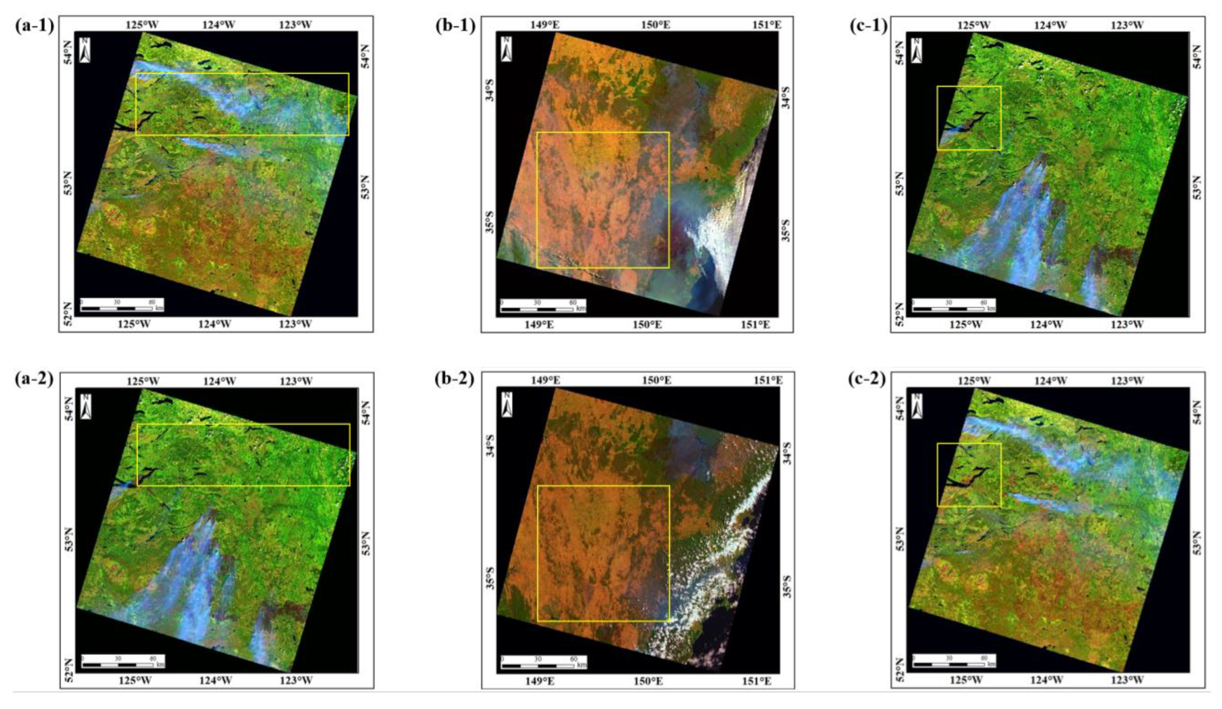
Figure 1. Satellite image of the study area for smoke/smoke-free samples, imagery color composition: 652 (RGB). The yellow boxes in the figure represent the regions where the samples are selected. (a-1,a-2) Vegetation: Landsat 8/OLI images of British Columbia, Canada on 7 August 2018 (a-1) and 4 August 2017 (a-2); (b-1,b-2) Soil: Landsat 8/OLI images of New South Wales, Australia on 31 December 2019 (b-1) and 15 December 2019 (b-2); (c-1,c-2) Water: Landsat 8/OLI images of British Columbia, Canada on 4 August 2017 (c-1) and 7 August 2018 (c-2).
Remotesensing 17 03880 g001
Figure 2. Satellite image of the study area for cloud/cloud-free samples, imagery color composition: 652 (RGB). The yellow boxes in the figure represent the regions where the samples are selected. (a-1,a-2) Vegetation: Landsat 8/OLI images of Victoria, Australia on 16 February 2020 (a-1) and 30 December 2019 (a-2); (b-1,b-2) Soil: Landsat 8/OLI images of New South Wales, Australia on 15 January 2020 (b-1) and 31 January 2020 (b-2); (c-1,c-2) Water: Landsat 8/OLI images of Victoria, Australia on 24 February 2020 (c-1) and 9 January 2021 (c-2).
Remotesensing 17 03880 g002
Figure 3. Spectral curves of smoke and clouds. The figure shows the mean spectral curves of smoke at varying concentration levels and clouds at varying thickness levels under vegetation (a), soil (b), and water (c) underlying surfaces. In the figure, Smoke 1 represents the mean of light smoke samples, and Smoke 5 represents the mean of thick smoke samples, with the sample concentration increasing sequentially as the number increases. Cloud 1 represents the mean of thin cloud samples, and Cloud 5 represents the mean of thick cloud samples, with the sample thickness increasing sequentially as the number increases.
Remotesensing 17 03880 g003
Figure 4. ANOVA results chart of smoke and clouds. ANOVA F -value results for different smoke concentrations and different cloud thicknesses under vegetation (a), soil (b), and water (c) underlying surfaces.
Remotesensing 17 03880 g004
Figure 5. Partial spectral curves and ANOVA results of selected smoke and clouds. (ac) Spectral curves of smoke samples at five concentration levels and cloud samples at levels 1–2 under vegetation (a), soil (b), and water (c) underlying surfaces; (d) Vegetation: ANOVA results for Cloud 1–Smoke 3 and Cloud 2–Smoke 5; (e) Soil: ANOVA results for Cloud 1–Smoke 2; (f) Water: ANOVA results for Cloud 1–Smoke 3.
Remotesensing 17 03880 g005
Figure 6. Two-dimensional scatter plots and frequency distribution histograms of smoke and cloud samples based on single bands under different underlying surfaces. (a-1a-5) Vegetation; (b-1b-5) Soil; (c-1c-5) Water. The scatter plot has x and y axes representing the bands, showing the relationship between smoke and cloud point clusters in the two-dimensional spectral space. The histogram at the top shows the frequency distribution of smoke and cloud samples corresponding to the x-axis, along with the normal distribution curve. The histogram on the right shows the frequency distribution of smoke and cloud samples corresponding to the y-axis, also with the normal distribution curve.
Remotesensing 17 03880 g006aRemotesensing 17 03880 g006b
Figure 7. VBI frequency distribution histograms of smoke and clouds under different underlying surfaces. (a) Vegetation; (b) Soil; (c) Water.
Remotesensing 17 03880 g007
Figure 8. Two-dimensional index scatter plots and frequency distribution histograms of smoke and cloud samples based on the ratio index under different underlying surfaces. (a-1a-3) Vegetation; (b-1b-3) Soil; (c-1c-3) Water. The scatter plot has x and y axes representing the ratio indices, showing the relationship between smoke and cloud point clusters in the two-dimensional index space. The histogram at the top shows the frequency distribution of smoke and cloud samples corresponding to the x-axis, along with the normal distribution curve. The histogram on the right shows the frequency distribution of smoke and cloud samples corresponding to the y-axis, also with the normal distribution curve.
Remotesensing 17 03880 g008aRemotesensing 17 03880 g008b
Figure 12. Satellite image of New South Wales, Australia on 31 December 2019 and the results of smoke and cloud recognition under different underlying surfaces. Imagery color composition: 432 (RGB). Among them, (a-1a-5,b-1b-5) Soil; (c-1c-5) Vegetation; (d-1d-5) Water; (a-1d-1) The locally enlarged images of the corresponding areas; (a-2d-2) The underlying surface images; (a-3d-3) The recognition results based on the MD method; (a-4d-4) The recognition results based on the random forest (RF) classification method; (a-5d-5) The recognition results based on the FSCRI method.
Remotesensing 17 03880 g012
Table 1. Interpretation symbols for smoke and smoke-free samples over different underlying surfaces. In this table, Level 1 represents light smoke. The texture of the underlying surface (such as vegetation canopy, soil furrows, and water waves) is clearly visible. The image color closely matches that of the pure underlying surface, with the type of ground objects only slightly obscured. Level 2 represents relatively light smoke. The texture of the underlying surface is blurred but still recognizable, and the basic color tone of the underlying surface remains identifiable. Level 3 represents medium-concentration smoke. The texture of the underlying surface is invisible, and the type of the underlying surface can only be roughly inferred from color. Level 4 represents relatively thick smoke. The type of the underlying surface is difficult to identify. The smoke is uniformly grayish-white, similar to thin clouds, but with more dispersed boundaries, and it often occurs around thick smoke. Level 5 represents thick smoke, which completely covers the underlying surface. The smoke is bright white with high reflectivity and typically occurs near the fire point. Smoke-free samples are representative underlying surface images from the site where the smoke samples were selected.
VegetationSoilWater
LevelSmokeSmoke-freeSmokeSmoke-freeSmokeSmoke-free
1Remotesensing 17 03880 i001Remotesensing 17 03880 i002Remotesensing 17 03880 i003Remotesensing 17 03880 i004Remotesensing 17 03880 i005Remotesensing 17 03880 i006
2Remotesensing 17 03880 i007Remotesensing 17 03880 i008Remotesensing 17 03880 i009Remotesensing 17 03880 i010Remotesensing 17 03880 i011Remotesensing 17 03880 i012
3Remotesensing 17 03880 i013Remotesensing 17 03880 i014Remotesensing 17 03880 i015Remotesensing 17 03880 i016Remotesensing 17 03880 i017Remotesensing 17 03880 i018
4Remotesensing 17 03880 i019Remotesensing 17 03880 i020Remotesensing 17 03880 i021Remotesensing 17 03880 i022Remotesensing 17 03880 i023Remotesensing 17 03880 i024
5Remotesensing 17 03880 i025Remotesensing 17 03880 i026Remotesensing 17 03880 i027Remotesensing 17 03880 i028Remotesensing 17 03880 i029Remotesensing 17 03880 i030
Table 2. Interpretation symbols for cloud and cloud-free samples over different underlying surfaces. In this table, Level 1 represents thin clouds, which appear semi-transparent, with details and contours of the underlying surface clearly visible. Level 2 represents relatively thin clouds, where surface details appear blurred, but the type of underlying surface can still be distinguished. Level 3 represents medium-thickness clouds, where surface details are completely obscured, but the clouds themselves are not highly bright and exhibit a gray tone. Level 4 represents relatively thick clouds, which are bright and appear in a light white color, typically located at the edges of large, dense cloud masses. Level 5 represents thick clouds, where the cloud surface may exhibit raised textures, and light is completely unable to penetrate, generally found in the central areas of large cloud masses. Cloud-free samples are representative underlying surface images from the site where the cloud samples were selected.
VegetationSoilWater
LevelCloudCloud-freeCloudCloud-freeCloudCloud-free
1Remotesensing 17 03880 i031Remotesensing 17 03880 i032Remotesensing 17 03880 i033Remotesensing 17 03880 i034Remotesensing 17 03880 i035Remotesensing 17 03880 i036
2Remotesensing 17 03880 i037Remotesensing 17 03880 i038Remotesensing 17 03880 i039Remotesensing 17 03880 i040Remotesensing 17 03880 i041Remotesensing 17 03880 i042
3Remotesensing 17 03880 i043Remotesensing 17 03880 i044Remotesensing 17 03880 i045Remotesensing 17 03880 i046Remotesensing 17 03880 i047Remotesensing 17 03880 i048
4Remotesensing 17 03880 i049Remotesensing 17 03880 i050Remotesensing 17 03880 i051Remotesensing 17 03880 i052Remotesensing 17 03880 i053Remotesensing 17 03880 i054
5Remotesensing 17 03880 i055Remotesensing 17 03880 i056Remotesensing 17 03880 i057Remotesensing 17 03880 i058Remotesensing 17 03880 i059Remotesensing 17 03880 i060
Table 3. FCSRI and thresholds for different underlying surfaces.
Underlying SurfacesFisher Smoke and Cloud Recognition IndexThreshold (T)
VegetationFSCRIV-14567 = −18.621 × b1 − 13.948 × b4 + 6.780 × b5 − 15.566 × b6 + 28.874 × b71.2506
FSCRIV-17 = −1.95 × b1 + 16.077 × b71.1821
FSCRIV-27 = −2.032 × b2 + 16.095 × b71.1912
FSCRIV-37 = −1.915 × b3 + 15.914 × b71.2434
FSCRIV-56 = −0.17 × b5 + 8.434 × b61.2812
FSCRIV-67 = −7.503 × b6 + 21.779 × b70.8787
SoilFSCRIS-24567 = −6.479 × b2 − 11.065 × b4 + 25.226 × b5 − 19.043 × b6 + 17.534 × b7−4.208
FSCRIS-17 = 4.477 × b1 − 7.693 × b7−0.9624
FSCRIS-27 = 4.741 × b2 − 7.792 × b7−0.7251
FSCRIS-37 = 4.961 × b3 − 7.943 × b7−0.56
FSCRIS-56 = 5.699 × b5 − 6.94 × b6−0.4750
FSCRIS-67 = 25.757 × b6 − 32.996 × b70.608
WaterFSCRIW-2467 = −22.572 × b2 + 21.358 × b4 − 20.575 × b6 + 35.569 × b70.0043
FSCRIW-17 = −0.823 × b1 + 12.13 × b70.4394
FSCRIW-27 = −0.879 × b2 + 12.157 × b70.4448
FSCRIW-37 = −0.875 × b3 + 12.152 × b70.4514
FSCRIW-56 = 0.47 × b5 − 7.387 × b6−0.4404
FSCRIW-67 = −21.695 × b6 + 37.114 × b70.4746
Table 4. Confusion matrix of smoke and cloud predicted labels and actual labels for the FSCRI model under different underlying surfaces.
VegetationSoilWater
Actual LabelsActual LabelsActual Labels
Predicted LabelsSmokeCloudTotalSmokeCloudTotalSmokeCloudTotal
Smoke98710598111091002102
Cloud293952899109898
Total100100 100100 100100
Disclaimer/Publisher’s Note: The statements, opinions and data contained in all publications are solely those of the individual author(s) and contributor(s) and not of MDPI and/or the editor(s). MDPI and/or the editor(s) disclaim responsibility for any injury to people or property resulting from any ideas, methods, instructions or products referred to in the content.