Mass Change in Antarctica from 2002 to 2025 Using GRACE and GRACE-FO

Highlights

When using GRACE and GRACE-FO for mass change estimates in Antarctica, multiple different solutions can be used. We compared five different Level-2 solutions and found that they agree very well on both trend estimation and monthly mass change when using a point mass inversion method.

What are the main findings?

• The five different Level-2 solutions result in comparable mass change estimates for Antarctica, and the Glacial Isostatic Adjustment (GIA) error is the dominant error source in the trend estimation.
• We can observe a big mass accumulation in the East Antarctic Basins 12 and 13 during 2021, 2022, and 2023.

What is the implication of the main findings?

• When estimating mass change from GRACE and GRACE-FO, the choice of solution is a negligible error source compared to the GIA error.
• Mass change in Antarctica is not linear, and trend estimation is still dependent on the chosen timespan.

Abstract

Several Level-2 solutions for the GRACE(-FO) gravity field exist. We compare five of these solutions using a mascon inversion method to estimate gridded mass change in Antarctica from gravity field grids at orbit height. We compare the mass change for all of Antarctica, as well as for 27 drainage basins. All five solutions show consistent negative mass trends for the period between April 2002 and January 2025 and show a mass accumulation in the East Antarctic basins 12 and 13 during the years 2021, 2022, and the beginning of 2023 but also a rapid mass loss starting in May 2023. While there are regional differences, the error from the Glacial Isostatic Adjustment model exceeds the differences between the solutions looked at in this study.

1. Introduction

Since April 2002, the Gravity Recovery and Climate Experiment (GRACE) Satellite and its follow-on mission, GRACE-FO, have been measuring changes in the Earth’s gravity field [1]. This makes it possible to study mass changes in the Antarctic Ice Sheet (AIS) [2,3,4,5]. The AIS stores roughly 26.5 million km³ of frozen water, which is equivalent to a 57.9 m global sea-level rise [6]. The 2023 IMBIE consortium inter-comparison study [7] combined independent mass change estimates using GRACE(-FO), satellite altimetry, and Surface Mass Balance. They estimated the rates of ice sheet mass change for the AIS from 1992 to 2020 to be −92 ± 18 GT/year. In this study, we focus on the mass change measured by GRACE and GRACE-FO, and estimate a trend for the time period from April 2002 to January 2025, comparing different gravity field solutions.

GRACE and GRACE-FO are satellite pairs separated by roughly 200 km along-track, which measure their position, relative position, and non-gravitational acceleration. Different processing centres then use these measurements to estimate global gravity fields. These gravity fields are referred to as Level-2 data and are available in various temporal and spatial resolutions, typically in the form of spherical harmonic coefficients [8]. These coefficients can then be used to evaluate the gravitational potential of the Earth at any point on or above the Earth. Converting a change in gravitational potential to a change in mass is non-unique. We are using an inversion method where we evaluate the potential on a grid at orbit height and invert it to determine the mass change at ground level, taking into account Glacial Isostatic Adjustment (GIA) and elastic loading, and regularising to overcome both the spatial resolution and non-uniqueness issues [5]. This method enables us to constrain the spatial pattern of mass change by adjusting the grid spacing, grid area, and regularisation parameter during the inversion. The calibration of these parameters has been looked at in detail in [2]. The mentioned studies have investigated the influence of GIA, regularisation, and the choice of mass grid on the error budget; however, the influence of different Level-2 products has not been investigated.

The primary aim of this study is to quantify the impact of using different Level-2 products from different processing centres. Secondly, we aim to extend the time series of ice mass change in Antarctica using data from GRACE and GRACE-FO.

In this study, we estimate monthly ice mass changes and trends from April 2002 to January 2025 for five different GRACE and GRACE-FO gravity field solutions. We do this for both Antarctica as a whole and for 27 drainage basins (Zwally basins [9]). We first present the monthly Level-2 data used and discuss the inversion method along with the corrections applied for elastic loading and GIA. In the Results section, we present the estimated trend for the entire Antarctica, as well as on a basin scale, and the monthly mass change. An analysis of the results is presented in the discussion.

2. Materials and Methods

2.1. Data

For this study, the Level-2 GRACE (RL06.0) and GRACE-FO (RL06.3) data from the three Science Data System analysis centres—Center for Space Research (CSR) [10,11], GeoForschungs Zentrum (GFZ) [12,13], and Jet Propulsion Laboratory (JPL) [14,15]—are used. We compare these results to the independent solution of the centre at the Technical University of Graz (ITSG2018) [16,17], and the combination product of the International Combination Service for Time-variable Gravity Fields (COST-G RL02.0) [18]. These gravity fields, expressed in spherical harmonic coefficients, are retrieved from the ICGEM service [8]. Following the recommendation by the analysis centres, the coefficients C20 and C30 are replaced by the Satellite Laser Ranging (SLR) solutions provided by NASA [19]. In this study, we use the degree 90 solutions but only use the first 60 degrees for the calculations.

2.2. From Spherical Harmonics to Mass Change

The method is described in more detail in [2,5]. To estimate mass change and mass trends from global gravity fields, we use a method based on inverting the gridded gravitational potential at orbit height to mass change at ground level. First, we calculate the gravity disturbance for each month on a grid at orbit height (480 km) using the spherical harmonic coefficients. The gravitational force is the gradient of the gravitational potential, and the gravity disturbance is the difference between the force and the normal ellipsoidal gravity. Using spherical coordinates with the origin at the centre of the Earth, the gravity disturbance at latitude $\varphi$, longitude $\lambda$, and height h above the surface is given by the derivative of the anomalous potential T [20]

$$\begin{array}{c}\delta g(R+h,\varphi ,\lambda )=-{\displaystyle \frac{\partial T}{\partial h}}={\displaystyle \frac{GM}{R^2}}\sum _{n=0}^N(n+1){\left({\displaystyle \frac{R}{R+h}}\right)}^{n+1}\sum _{m=0}^n((C_{nm}-C_{nm}^{normal})\cos \left(m\lambda \right)\hfill \\ \hfill +S_{nm}\sin \left(m\lambda \right))P_{nm}\left(\sin \varphi \right),\end{array}$$

(1)

with the gravitational constant G, the Earth’s mass M, and the Earth’s radius R. The spherical harmonic coefficients $C_{nm}$ and $S_{nm}$ are the provided Level-2 data, and the coefficients of the normal gravity $C_{nm}^{normal}$ are given in [20]. The associated Legendre functions $P_{nm}$ are defined recursively. Since we are studying ice mass change, we also need to account for elastic loading, the response of the Earth’s crust to changes in ice mass as seen in [21]. This is performed by applying corrections to the anomalous spherical harmonic coefficients using the elastic Love numbers $k_n$ [21]

$$C_{nm}^{*}={\displaystyle \frac{1}{1+k_n}}(C_{nm}-C_{nm}^{normal}),S_{nm}^{*}={\displaystyle \frac{1}{1+k_n}}{S}_{nm}.$$

(2)

Next, we estimate a trend and a yearly amplitude and phase for each grid cell i at orbit height h as

$$\delta g_i^h\left(t\right)=b_i+c_i\ast (t-t_0)+A_i\sin (t-t_0)+B_i\cos (t-t_0),$$

(3)

where $\delta g_i^h\left(t\right)$ is the gravity disturbance at orbit height h for grid cell i, $b_i$ is the bias, $c_i$ the trend, $A_i^2+B_i^2$ the amplitude, and $\arctan \left({\displaystyle \frac{A_i}{B_i}}\right)$ is the phase for each grid cell. This results in a gridded estimate for the trend in gravity disturbance at orbit height.

Lastly, we invert the gridded trend and the monthly grids to mass change on the ground using Newton’s law of gravitation (see e.g., [20]). The radial component of the attraction between a point i on the orbit and a point mass $m_j$ on the ground is a function of the distance between the two points. Expressing this distance as a function of orbit height h, Earth radius R, radius $r=R+h$, and spherical distance $\psi$ results in [5,20]

$$\delta g_i=G\delta m_j{\displaystyle \frac{R^{2}r-R^3\cos {\psi }_{ij}}{{(r^2+R^2-2Rrcos{\psi }_{ij})}^{3/2}}},$$

(4)

where i refers to the grid at orbit height and j to the grid on the ground. $\delta g_i$ is either the trend in gravity disturbance (see Equation (3)) or monthly gravity disturbance grids (relative to the first epoch). In both of these cases, $\delta g_i$ describes a change in gravity disturbance. The mass grids $\delta m_j$ are thus either mass trends or mass change relative to the first month. Defining the observation vector $\mathbf{y}=\left\{\delta g_i\right\}$ and the solution vector $\mathbf{x}=\left\{\delta m_j\right\}$, we can write Equation (4) as a matrix equation

$$\mathbf{y}=\mathbf{A}\mathbf{x},$$

(5)

which we solve by generalised inverse using the Tikhonov regularisation

$$\mathbf{x}={({\mathbf{A}}^T\mathbf{A}+{\displaystyle \frac{1}{\kappa }}\mathbf{I})}^{-1}{\mathbf{A}}^T\mathbf{y}.$$

(6)

The regularisation factor ${\displaystyle \frac{1}{\kappa }}$ constrains the model and reduces noise, but it also reduces the signal content. The choice of $\kappa$ affects the inevitable trade-off between residuals and the smoothness of the model. The choice of the regularisation parameter is made based on an L-curve and is discussed in Appendix A. The choice of the regularisation parameter does affect both the amplitude of the measured mass change and the spatial distribution. When choosing a regularisation parameter around the “knee” of the L-curve, the variation of the total trend estimation is negligible (see Figure A2). The choice of grids, both at orbit level and ground level, and the choice of maximum degree also affect the mass change estimation [2]. In this study we uses polar stereographic grids with a grid spacing of 100 km on ground. The grid at orbit height is chosen to be slightly larger than the extent of Antarctica and for the grid on ground, only gridpoints inside the Zwally Basins and an ocean band 500 km away from the coast are selected as point masses for the inversion. While we use the degree 90 Level-2 solutions, we only evaluate the spherical harmonic coefficients up to degree 60. The calibration of these choices is not performed for this study, and the choices are made based on [2]. This does not affect the comparability of solutions.

The Level-2 solutions also provide formal errors for the spherical harmonic coefficients. Using Monte Carlo simulations, these formal errors are propagated to the mass trend and monthly mass change estimates. This is achieved by generating 100 distinct sets of spherical harmonic coefficients for each solution, using random numbers. These are then inverted to monthly mass change and trend estimations following the above method. Finally, the mean and standard deviation are calculated for each month and for the trend. This contribution to the error is referred to as a “formal error” below.

The time series of spherical harmonic coefficients includes all the signals related to moving mass, including ice mass change, hydrology, and Glacial Isostatic Adjustment (GIA), among others. Since we are not interested in measuring the GIA in this study, we need to remove this signal. To remove the GIA signal, we use gravity disturbance trends at orbit height derived from Geoid height trends of the W12a GIA model by [22]. As shown in the IMBIE study [7], the choice of the GIA model affects the ice mass solutions significantly and is a big error source. To quantify this error, the calculation is performed for each solution with the three GIA scenarios (lower bound, best fit, and upper bound) provided by W12a [22]. This choice is based on [23], where they calculated the mass trend using 10 different GIA models and found that the mean and standard deviation of all continent-wide models are very close to the W12a. Other models, such as ICE-6G or IJ05_R2, would change the monthly mass change, especially at the end of the period and the trend estimation. The comparison of the different solutions does not depend on the choice of the GIA model as long as the same one is used.

3. Results

We present the monthly mass changes at the drainage basin scale and for Antarctica as a whole, and estimate a mass trend from April 2002 to January 2025.

3.1. Trends

We estimate trends for all solutions for the Zwally drainage basins [9] between April 2002 and January 2025. Figure 1a shows the estimated trend for the combination solution COST-G with mass gain in red and mass loss in blue. Figure 1b illustrates the error associated with the GIA model. Figure 1c shows the standard deviation between all five solutions. The numbers are the Zwally drainage basin numbers. Figure 2 shows the estimated trend per basin and solution including the estimated trend for the whole of Antarctica for every solution using the “best fit” GIA scenario and the GIA error (−7.8 GT/year when using the upper bound on GIA scenario to +12.9 GT/year for the lower bound GIA scenario) as a table and also includes the standard deviation between all five solutions. Using Monte Carlo simulations, the formal errors of the spherical harmonic coefficients result in an error of about $\pm 0.7$ GT/year for the total trend. As this is much smaller than the GIA error, it is neglected in Figure 1 and Figure 2. We also do not provide a measure for the goodness of fit, as the estimation of the trend is made for the gravity disturbance grids at orbit height before inverting to mass trend grids.

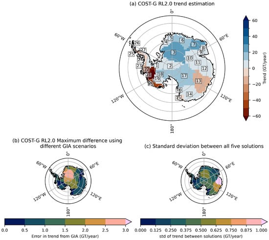
Figure 1. (a) Trend estimation of mass change for Antarctica on basin scale for the combination product COST-G RL2.0. The numbers are the Zwally basin numbers. (b) Maximum difference in the estimated trends when using COST-G RL2.0 and the three different GIA scenarios. (c) Standard deviation between all five solutions.

Figure 2. Trend estimation of mass change for Antarctica on basin scale for all GRACE(-FO) solutions considered in this study. The numbers show the estimated trend using the “best fit” GIA model (number to the left) and the difference when using the upper-bound GIA uplift model (upper right) and the lower-bound GIA uplift model (lower right).

3.2. Monthly Mass Change

The monthly mass change for the period from April 2002 to January 2025 for the whole of Antarctica is shown in Figure 3. Figure 3a shows the mean of the monthly mass change based on all five solutions, as well as the GIA error and errors from formal errors in spherical harmonic coefficients, trend estimation, and GIA error in trend. For comparison, the results of IMBIE2021 [7] are included. Figure 3b shows the difference from the mean for all five solutions, where the mean is removed from each solution. Figure 3c shows the upper and lower bounds of the GIA error (lines) and the error from the formal errors. Figure 3d–f show the comparison between the IMBIE2021 and this study for the East Antarctic Ice Sheet (EAIS), the West Antartic Ice Sheet (WAIS) and the Antarctic Peninsula (API). This figure shows the non-linear nature of the mass change in Antarctica during the GRACE-FO period. The error from formal errors in the spherical harmonic coefficients is almost invisible during the first 10 years of the observation period but increases in the second half of the GRACE period and stays higher during the GRACE-FO period. This is likely due to battery saving mode for the GRACE accelerometer during the last months of the mission [24] and problems with the GRACE-FO accelerometer [25]. The GIA error, which is an error in uplift rates, increases linearly over the full observation period. The mean difference from the mean is calculated for all five solutions, showing that CSR RL6.3, GFZ RL6.3, and JPL RL6.3 generally estimate a higher mass balance (lower mass loss), and ITSG2018 and COST-G estimate a lower mass balance (higher mass loss).

Figure 3. Monthly mass change relative to the first epoch for the whole of Antarctica. (a) The mean of four independent solutions (black dots, not including COST-G RL2), the error from the formal errors (dark grey) in the spherical harmonic coefficients, and the GIA error (light grey) based on the three different uplift scenarios provided by [22]. The trend is the mean trend for CSR RL6.3, GFZ RL6.3, JPL RL6.3 and ITSG2018, shown in Figure 2 with the upper and lower bounds based on the different GIA scenarios. (b) The difference between each solution and the mean. The darker area shows the formal error, while the lighter area is the GIA error. (c) The GIA error (dashed line) and the formal error (dots) for each of the five solutions. The remaining figures show the monthly mass change compared to the IMBIE 2021 study for the three regions (d) East Antarctica, (e) West Antarctica and (f) Antarctic Peninsula.

Figure 4 shows a selection of monthly solutions on basin scale. The rest of the monthly solutions for every basin are provided in Appendix B. The mean of the monthly mass change (relative to the first epoch) based on the independent Level-2 solutions CSR RL6.3, GFZ RL6.3, JPL RL6.3, and ITSG2018 and the trend based on these solutions are shown in the left figures. The difference from the mean for all five solutions is shown on the right. The plots include the GIA error (lighter area) and the error from the formal errors (darker area). These plots show the following basins. Basin 2 shows a small mass trend with inconsistent signs for the different solutions and one of the higher GIA errors (see Figure 2). Basin 3 has the biggest positive mass trend and displays the biggest GIA error. Basin 13 has the biggest negative trend on the EAIS. Basin 17 shows a positive trend and a big GIA error, and Basin 21 has the biggest negative trend in the whole of Antarctica.

Figure 4. Monthly mass change relative to the first epoch for five basins. The left figures show the mean of four independent solutions (not including COST-G RL2), the error from the formal errors in the spherical harmonic coefficients and the GIA error based on the three different uplift scenarios provided by [22]. The linear mass change (blue) is calculated using the mean trend for CSR RL6.3, GFZ RL6.3, JPL RL6.3, and ITSG2018 shown in Figure 2 with the upper and lower bounds based on the different GIA scenarios. The right figures show the difference between each solution and the mean. The darker areas show the formal error, while the lighter areas are the GIA error.

4. Discussion

The estimated trend in Figure 1 and Figure 2 is consistent in sign for all five solutions for most basins. Only basin 2 shows differences in the sign of the trend between solutions. This basin shows a trend close to zero, and the GIA error is bigger than the difference between all solutions. Basin2 is at the border to the West Antarctic Ice Sheet (WAIS), and thus leakage effects might be the reason for this sign change. This difference in sign is thus not an indication that the choice of the Level-2 solution significantly affects the estimated trend.

The GIA error is almost the same for all five solutions. This is expected, as we are using the same GIA model in the processing of these five solutions. The difference between Level-2 solutions exceeds the GIA error in basins 9, 11, 12, 13, 14, 24 and 26. Basins 9 and 11 are very small basins at the edge of the East Antarctic Ice Sheet (EAIS), making them more affected by ringing noise (see Figure A3 in Appendix A), and the GIA error is especially small for basins 9 and 11. The GFZ RL6.3 solution shows a lower amplitude in the trend than the remaining solutions in basin 12 and 13 and a higher mass gain in basin 14. Basins 24 and 26 are on the Antarctic Peninsula (API) which is very narrow and also affected by the increased noise along the coast. In general, GFZ RL6.3 displays higher mass gain and lower mass loss trends. This is visible in the total mass loss trend, which is between 2.3 GT/year and 3.1 GT/year lower than the other four solutions.

Looking at the monthly mass change in Figure 3, we observe that all five solutions show a big mass accumulation in the second half of 2022 and beginning of 2023 but also a big melt event starting between April and May 2023 and again in the second half of 2024. At the end of the GRACE period during 2017, the ITSG2018 solution deviates from the three other independent solutions, CSR RL6.3, GFZ RL6.3 and JPL RL6.3. Usually, the ITSG2018 solution exhibits very low noise, which is also reflected in the COST-G combination, which often gives it a high weight [26]. The COST-G service provides a tool to plot the RMS over the oceans, which is a measure for how noisy a solution is [27]. Based on this, the ITSG2018 solution shows more noise at the end of the GRACE mission. Therefore, we do not use the data from 2017 to estimate the trend.

We also compare our monthly mass balance with the results from the IMBIE2021 results [7]. While the trends of this study cannot be compared directly to the trends in [7] due to different time periods, the monthly mass change estimates on both continental and regional scales are included in Figure 3. The mass gain of the EAIS is estimated to be higher in this study than in the IMBIE dataset, which also affects the total mass balance. In [23], the estimated trend for the EAIS during the period of 1992–2017 is 5 ± 46 GT/year, showing that this region has big uncertainties.

Next, we look at the monthly mass change for the five basins in Figure 4. The monthly mass balance for basin 2 shows a small mass change over the total period, with a relatively big GIA error, and while all solutions agree on the trend, there is a small offset in the mass balance relative to the first epoch.

Basin 3 shows a clear trend and a big difference between the “best fit” GIA solution and the upper bound coming from the minimum GIA rate scenario. While the GFZ RL6.3 solution shows a different behaviour at the end of the GRACE mission, the trend estimation for the whole time period is consistent for all five solutions.

Basin 13 is one of the basins on the EAIS with a negative trend. The monthly mass change shows the mass loss starting at around 2012 and a mass gain between 2022 and 2023. But there is also an estimated mass loss since the peak in 2023, resulting in a net negative mass balance. This mass gain and subsequent mass loss is also seen in the neighbouring basins (see Appendix B) and is big enough to also be reflected in the mass balance for the whole of Antarctica (see Figure 3). This basin is one where the upper bound of GIA uplift rates shows a larger difference from the “best fit” GIA scenario.

Basin 17 does not display a linear trend but rather three steps in mass gain with periods of minimal mass change from 2002 to 2011, from 2011 to 2017 and from 2018 to 2025 with a positive mass balance over all.

Basin 21 is one of the basins on the WAIS with a strong negative trend and is an example of a strong signal where all solutions agree, and the GIA error is relatively small compared to the actual signal (less than 2%, see Figure 2). While the total mass loss over the whole period is estimated to be about 1500 GT, the difference between the solutions is of the order of ±50 GT (not including the year 2017), and when taking the GIA error into account, the error in mass balance towards the end of the observation period increases to the order of ±100 GT.

5. Conclusions

In this study, we looked at five gravity field solutions covering more than twenty years of GRACE and GRACE-FO data and calculated the mass change using these five solutions. We estimated the trend in mass change in Antarctica and investigated whether the different gravity field solutions agree with each other. All five solutions show a clear negative trend and lie within the GIA error of each other with a small exception for ITSG2018 at the end of the GRACE mission in 2017. GFZ RL6.3 differs the most from the other solutions in general. In some cases, the choice of processing centre can influence the derived mass trend on basin scale. Nonetheless, for the entire continent of Antarctica, the GIA error is the dominant error source when estimating both trend and monthly mass balance over long time periods.

The main mass loss occurs on the West Antarctic Ice Sheet (WAIS), while the East Antarctic Ice Sheet (EAIS) is more stable and gains mass in some regions. These results are consistent with those in the study by the IMBIE consortium [28], while the estimated trends cannot be compared directly due to different time periods.

Looking at the monthly mass change in all the basins separately, we identified a big mass accumulation event in basin 13 in June, July, and August 2022. This mass accumulation is also visible in the time series for the entire Antarctica in Figure 3 and is not yet part of the IMBIE study mentioned above. This is also an example of a basin that does not show a linear mass loss, demonstrating that when examining mass trends on a basin scale, it is important to also consider the monthly time series, as not all basins display a linear mass change.

References

- Tapley, B.D.; Bettadpur, S.; Watkins, M.; Reigber, C. The gravity recovery and climate experiment: Mission overview and early results. Geophys. Res. Lett. 2004, 31, L09607. [Google Scholar] [CrossRef]
- Barletta, V.R.; Sørensen, L.S.; Forsberg, R. Scatter of mass changes estimates at basin scale for Greenland and Antarctica. Cryosphere 2013, 7, 1411–1432. [Google Scholar] [CrossRef]
- Shepherd, A.; Ivins, E.R.; Geruo, A.; Barletta, V.R.; Bentley, M.J.; Bettadpur, S.; Briggs, K.H.; Bromwich, D.H.; Forsberg, R.; Galin, N.; et al. A reconciled estimate of ice-sheet mass balance. Science 2012, 338, 1183–1189. [Google Scholar] [CrossRef] [PubMed]
- Groh, A.; Horwath, M.; Horvath, A.; Meister, R.; Sørensen, L.S.; Barletta, V.R.; Forsberg, R.; Wouters, B.; Ditmar, P.; Ran, J.; et al. Evaluating GRACE mass change time series for the Antarctic and Greenland ice sheet—Methods and results. Geosciences 2019, 9, 415. [Google Scholar] [CrossRef]
- Forsberg, R.; Sørensen, L.; Simonsen, S. Greenland and Antarctica ice sheet mass changes and effects on global sea level. In Integrative Study of the Mean Sea Level and Its Components; Cazenave, A., Champollion, N., Paul, F., Benveniste, J., Eds.; Springer International Publishing: Cham, Switzerland, 2017; pp. 91–106. [Google Scholar] [CrossRef]
- Morlighem, M.; Rignot, E.; Binder, T.; Blankenship, D.; Drews, R.; Eagles, G.; Eisen, O.; Ferraccioli, F.; Forsberg, R.; Fretwell, P.; et al. Deep glacial troughs and stabilizing ridges unveiled beneath the margins of the Antarctic ice sheet. Nat. Geosci. 2020, 13, 132–137. [Google Scholar] [CrossRef]
- Otosaka, I.N.; Shepherd, A.; Ivins, E.R.; Schlegel, N.J.; Amory, C.; van den Broeke, M.R.; Horwath, M.; Joughin, I.; King, M.D.; Krinner, G.; et al. Mass balance of the Greenland and Antarctic ice sheets from 1992 to 2020. Earth Syst. Sci. Data 2023, 15, 1597–1616. [Google Scholar] [CrossRef]
- Ince, E.S.; Barthelmes, F.; Reißland, S.; Elger, K.; Förste, C.; Flechtner, F.; Schuh, H. ICGEM – 15 years of successful collection and distribution of global gravitational models, associated services, and future plans. Earth Syst. Sci. Data 2019, 11, 647–674. [Google Scholar] [CrossRef]
- Zwally, H.J.; Giovinetto, M.B.; Beckley, M.A.; Saba, J.L. Antarctic and Greenland Drainage Systems; GSFC Cryospheric Sciences Laboratory: Greenbelt, MD, USA, 2012.
- University of Texas Center for Space Research (UTCSR). GRACE Static Field Geopotential Coefficients CSR Release 6.0; Dataset, NASA Physical Oceanography Distributed Active Archive Center: Pasadena, CA, USA, 2018. [CrossRef]
- GRACE-FO. GRACE-FO Level-2 Monthly Geopotential Spherical Harmonics CSR Release 06.3 (RL06.3); Dataset, NASA Physical Oceanography Distributed Active Archive Center: Pasadena, CA, USA, 2024. [CrossRef]
- Dahle, C.; Flechtner, F.; Murböck, M.; Michalak, G.; Neumayer, H.; Abrykosov, O.; Reinhold, A.; König, R. GRACE Geopotential GSM Coefficients GFZ RL06, Version 6.0; Dataset, GFZ Data Services: Potsdam, Germany, 2018. [CrossRef]
- Dahle, C.; Flechtner, F.; Murböck, M.; Michalak, G.; Neumayer, H.; Abrykosov, O.; Reinhold, A.; König, R. GRACE-FO Geopotential GSM Coefficients GFZ RL06, Version 6.3; Dataset, GFZ Data Services: Potsdam, Germany, 2019. [CrossRef]
- NASA Jet Propulsion Laboratory. GRACE Static Field Geopotential Coefficients JPL Release 6.0; Dataset, NASA Physical Oceanography Distributed Active Archive Center: Pasadena, CA, USA, 2018. [CrossRef]
- GRACE-FO. GRACE-FO Level-2 Monthly Geopotential Spherical Harmonics JPL Release 6.3; Dataset, NASA Physical Oceanography Distributed Active Archive Center: Pasadena, CA, USA, 2024. [CrossRef]
- Mayer-Gürr, T.; Behzadpour, S.; Ellmer, M.; Kvas, A.; Klinger, B.; Strasser, S.; Zehentner, N. ITSG-Grace2018—Monthly, Daily and Static Gravity Field Solutions from GRACE; Dataset, GFZ Data Services: Potsdam, Germany, 2018. [Google Scholar] [CrossRef]
- Kvas, A.; Behzadpour, S.; Ellmer, M.; Klinger, B.; Strasser, S.; Zehentner, N.; Mayer-Gürr, T. ITSG-Grace2018: Overview and evaluation of a new GRACE-only gravity field time series. J. Geophys. Res. Solid Earth 2019, 124, 9332–9344. [Google Scholar] [CrossRef]
- Meyer, U.; Jäggi, A.; Dahle, C.; Flechtner, F.; Kvas, A.; Behzadpour, S.; Öhlinger, F.; Mayer-Gürr, T.; Lemoine, J.M.; Bourgogne, S.; et al. International Combination Service for Time-Variable Gravity Fields (COST-G) Monthly GRACE/GRACE-FO RL02 Series, Version 2; Dataset, GFZ Data Services: Potsdam, Germany, 2025. [CrossRef]
- Loomis, B.D.; Rachlin, K.E.; Wiese, D.N.; Landerer, F.W.; Luthcke, S.B. Replacing GRACE/GRACE-FO With Satellite Laser Ranging: Impacts on Antarctic Ice Sheet Mass Change. Geophys. Res. Lett. 2020, 47, e2019GL085488. [Google Scholar] [CrossRef]
- Hofmann-Wellenhof, B.; Moritz, H. Physical Geodesy; Springer Science & Business Media: Berlin/Heidelberg, Germany, 2006. [Google Scholar] [CrossRef]
- Wahr, J.; Molenaar, M.; Bryan, F. Time variability of the Earth’s gravity field: Hydrological and oceanic effects and their possible detection using GRACE. J. Geophys. Res. Solid Earth 1998, 103, 30205–30229. [Google Scholar] [CrossRef]
- Whitehouse, P.L.; Bentley, M.J.; Le Brocq, A.M. A deglacial model for Antarctica: Geological constraints and glaciological modelling as a basis for a new model of Antarctic glacial isostatic adjustment. Quat. Sci. Rev. 2012, 32, 1–24. [Google Scholar] [CrossRef]
- Team, I. Mass balance of the Antarctic ice sheet from 1992 to 2017. Nature 2018, 558, 219–222. [Google Scholar] [CrossRef] [PubMed]
- Bandikova, T.; McCullough, C.; Kruizinga, G.L.; Save, H.; Christophe, B. GRACE accelerometer data transplant. Adv. Space Res. 2019, 64, 623–644. [Google Scholar] [CrossRef]
- McCullough, C.M.; Harvey, N.; Save, H.; Bandikova, T. Description of Calibrated GRACE-FO Accelerometer Data Products (ACT), Level-1 Product Version 04, Technical report; NASA Jet Propulsion Laboratory/California Institute of Technology: La Cañada Flintridge, CA, USA, 2019.
- Meyer, U.; Lasser, M.; Dahle, C.; Förste, C.; Behzadpour, S.; Koch, I.; Jäggi, A. Combined monthly GRACE-FO gravity fields for a global gravity-based groundwater product. Geophys. J. Int. 2023, 236, 456–469. [Google Scholar] [CrossRef]
- International Combination Service for Time-Variable Gravity Fields (COST-G). COST-G Monthly GRACE/GRACE-FO RL02 Series—Statistics Plot. 2025. Available online: https://plot.cost-g.org/statistics/ (accessed on 12 November 2025).
- Otosaka, I.N.; Horwath, M.; Mottram, R.; Nowicki, S. Mass balances of the Antarctic and Greenland ice sheets monitored from space. Surv. Geophys. 2023, 44, 1–38. [Google Scholar] [CrossRef]
Disclaimer/Publisher’s Note: The statements, opinions and data contained in all publications are solely those of the individual author(s) and contributor(s) and not of MDPI and/or the editor(s). MDPI and/or the editor(s) disclaim responsibility for any injury to people or property resulting from any ideas, methods, instructions or products referred to in the content. |
© 2025 by the authors. Licensee MDPI, Basel, Switzerland. This article is an open access article distributed under the terms and conditions of the Creative Commons Attribution (CC BY) license (https://creativecommons.org/licenses/by/4.0/).