SF3Net: Frequency-Domain Enhanced Segmentation Network for High-Resolution Remote Sensing Imagery

Highlights

What are the main findings?

• SF3Net is proposed, which integrates frequency-domain enhancement and spatial aggregation for semantic segmentation of high-resolution remote sensing images, achieving a superior balance between accuracy and computational efficiency compared with state-of-the-art methods.
• Experimental results demonstrate that frequency-domain enhancement, spatial aggregation, and their fusion improve mIoU by 1.165%, 0.811%, and 1.436%, respectively, while effectively preserving boundary details and spatial structure integrity.

What are the implication of the main findings?

• Provides a high-precision tool for high-resolution remote sensing image segmentation, supporting urban planning and land management research that relies on accurate analysis of high-resolution imagery.
• Validates the effectiveness of frequency-domain strategies in high-resolution remote sensing and demonstrates the necessity of frequency–spatial fusion strategies, offering methodological reference for dual-domain fusion segmentation research.

Abstract

With the rapid development in semantic segmentation in remote sensing (RS) imagery, the balance between segmentation accuracy and computational efficiency has been recognized as a key challenge. Most existing approaches have predominantly been based on spatial features, while the potential of frequency-domain information has remained underexplored. To address this limitation, a Spatial-Frequency Feature Fusion Network (SF3Net) is proposed, aiming to achieve accurate segmentation with reduced computational cost. The framework is composed of two core modules: the Frequency Feature Stereo Learning (FFSL) module, designed to extract frequency features from multiple orientations, and the Spatial Feature Aggregation Module (SFAM), developed to enhance spatial feature representation. In addition, a Feature Selection Module (FSM) is incorporated to retain shallow features from the encoder, thereby compensating for detail loss during downsampling. Comprehensive experiments demonstrate the effectiveness of SF3Net: it achieves mean Intersection-over-Union (mIoU) scores of 80.040% and 83.934% on the ISPRS-Potsdam and ISPRS-Vaihingen datasets, respectively, and 88.657% on a self-constructed farmland dataset. These results consistently surpass those of state-of-the-art spatial–frequency fusion methods. Overall, SF3Net provides an efficient and effective paradigm for jointly modeling spatial and frequency-domain features in remote sensing semantic segmentation.

1. Introduction

With the rapid advancement in high-quality RS imaging technologies, the acquisition of large volumes of high-resolution RS imagery has become possible. At the same time, the progress of artificial intelligence and deep learning has provided powerful tools for analyzing such data. High-resolution RS images are capable of capturing detailed surface information and complex object characteristics, while also offering insights into ecological environments and human activities [1]. By extracting and analyzing relevant information from these images, a comprehensive understanding of natural environments and anthropogenic patterns can be achieved from multiple perspectives. This deeper understanding plays a critical role in supporting analysis, monitoring, and decision-making across a wide range of domains [2]. These capabilities have driven the application of RS semantic segmentation across several domains. In environmental monitoring, it supports land and water body segmentation [3] and disaster assessment [4]; in agricultural management, it enables farmland mapping [5] and crop yield estimation [6]; and in urban planning [7], it facilitates road extraction and infrastructure analysis [8]. Such diverse applications highlight the essential role of semantic segmentation in transforming raw RS imagery into actionable information for environmental assessment, resource management, and decision support.

Traditional image segmentation methods primarily rely on spectral, spatial, and textural features for segmenting RS images [9]. However, these approaches struggle to generalize to complex and diverse high-resolution RS data due to their dependence on handcrafted features and limited capacity for nonlinear representation. Consequently, their performance in large-scale and heterogeneous scenarios remains unsatisfactory. With the advent of deep learning, CNNs, Transformers, and Mamba have achieved remarkable progress in semantic segmentation of RS images. In recent years, CNNs have attained significant success in this field owing to their strong capability for local feature modeling. FCN [10], as a milestone in applying CNNs to image segmentation, substantially improved segmentation accuracy. Subsequently, U-Net [11], with its encoder–decoder architecture incorporating skip connections, has become a standard framework in image segmentation. Nevertheless, the inherent limitations of convolutional kernels restrict the receptive field, hindering the ability to capture long-range dependencies. To address this issue, CCNet [12] integrates a criss-cross attention module to capture long-distance contextual information. DANet [13] employs a dual attention mechanism to enhance the representation of features in both spatial and channel dimensions, thus improving the precision of segmentation. DeepLabv3 [14] combines dilated convolutions with an atrous spatial pyramid pooling (ASPP) structure, further enhancing performance. In addition, several studies have focused on alleviating boundary ambiguity. Ref. [15] replaced skip connections with boundary attention to more effectively restore the boundaries of objects. Ref. [16] incorporated boundary information for the multimodal fusion of characteristics, improving the accuracy of boundary segmentation. Ref. [17] proposed a novel prototype matching strategy for body joint boundaries to mitigate feature aliasing at object edges.

Although CNNs have achieved remarkable success in many computer vision tasks, they are inherently constrained by the limited receptive field of convolutional kernels, making it challenging to capture multi-scale features in RS images. Transformers [18], leveraging self-attention mechanisms, effectively capture global contextual information and demonstrate strong performance in modeling long-range dependencies. Ref. [19] proposed combining a pyramid structure with attention mechanisms to enhance the model’s ability to capture global information. Similarly, ref. [20] introduced lightweight attention modules that preserved global perception while reducing computational cost. However, Transformers often underperform in modeling fine-grained local details. To address this limitation, Swin Transformer [21] introduced a shifted window mechanism to capture multi-scale global features, achieving superior performance in fine-grained classification and boundary recognition. LGBSwin [22] further enhanced global modeling capability by integrating spatial and channel attention, adaptively fusing low- and high-level features to extract boundary information and mitigate boundary ambiguity. In addition, segmentation networks relying solely on CNNs are limited in capturing global representations, while pure Transformer-based networks tend to lose fine-grained local details. Consequently, researchers have increasingly explored hybrid architectures that integrate CNNs with Transformers. For instance, CCTNet [23] couples CNN and Transformer networks through a lightweight adaptive fusion module, effectively integrating local information with global context and demonstrating the effectiveness of hybrid models in RS image segmentation. LETNet [24] embeds Transformer and CNN components to complement each other’s limitations. DAFormer [25] and SegFormer [26] combine the local feature extraction strength of CNNs with the long-range dependency modeling capability of Transformers, delivering outstanding performance in semantic segmentation, particularly in complex and dynamic scenarios. In recent years, Mamba [27] has emerged as a research focus due to its excellent long-range modeling ability and linear computational complexity. VMamba [28] was the first to apply Mamba to image segmentation, verifying its effectiveness in vision tasks. RS3Mamba [29] adopted a dual-encoder structure with Mamba and CNN, significantly improving segmentation accuracy through feature fusion. Overall, existing Transformer-based or hybrid CNN-Transformer or Mamba architectures have demonstrated strong capabilities in capturing global contextual information and integrating multi-scale spatial features. However, these models primarily operate in the spatial domain and rarely exploit frequency-domain representations, limiting their ability to handle complex textures, fine boundaries, and noise-prone details commonly found in remote sensing images. This gap motivates our study to incorporate frequency-domain feature learning into the segmentation framework, aiming to achieve more balanced modeling of both spatial and frequency information for improved segmentation robustness and accuracy.

Frequency-domain techniques have attracted significant attention in RS image semantic segmentation due to their ability to effectively capture both global and local features. Methods such as Fourier and wavelet transforms decompose RS images into frequency components, enabling more efficient extraction of fine details and global structures. FcaNet [30] introduces a frequency channel attention mechanism that enhances feature selection by leveraging both spatial and frequency information to improve the performance of CNNs. XNet [31] employs a wavelet-based network to integrate low- and high-frequency features, thereby improving semantic segmentation of biomedical images in both fully supervised and semi-supervised settings through the joint use of spatial and frequency data. SpectFormer [32] incorporates frequency-domain information and attention mechanisms into the ViTs framework, enhancing its capability to handle visual tasks. In addition, SFFNet [33] adopts a spatial–frequency fusion network based on wavelets to effectively combine spatial and frequency information, thereby improving segmentation performance in remote sensing imagery. Moreover, RS images are often affected by high-frequency noise resulting from sensor limitations, atmospheric interference, and complex surface textures. Such noise overlaps with genuine high-frequency details, making it difficult to distinguish informative signals from irrelevant variations and often leading to degraded segmentation accuracy. To mitigate these effects, frequency-domain techniques have been introduced to enhance useful frequency information and suppress redundant components [34]. However, most existing approaches rely on one-dimensional frequency modeling, treating the frequency domain as an auxiliary enhancement rather than a primary representation. Their limited capacity for multi-dimensional frequency learning and lack of explicit noise suppression strategies can lead to the loss of critical spatial information, restricting their effectiveness in complex real-world scenarios.

Based on the above analysis, we propose a spatial–frequency feature fusion network (SF3Net) with a U-shaped encoder–decoder architecture. The network effectively integrates frequency domain features while preserving spatial features enriched with semantic information. Specifically, to effectively extract comprehensive frequency domain features, we propose the frequency feature stereoscopic learning module (FFSL), which utilizes Fourier transform to capture frequency information from three directions. Moreover, the spatial feature aggregation module (SFAM) enhances spatial contextual features through weighted extraction. Subsequently, the spatial–frequency feature fusion module (SFFM) integrates frequency domain features from FFSL with spatial features from SFAM, enabling comprehensive feature fusion. In addition, a feature selection module (FSM) is introduced to select the shallow features of the encoder to compensate for the loss of detail during the encoder downsampling process.

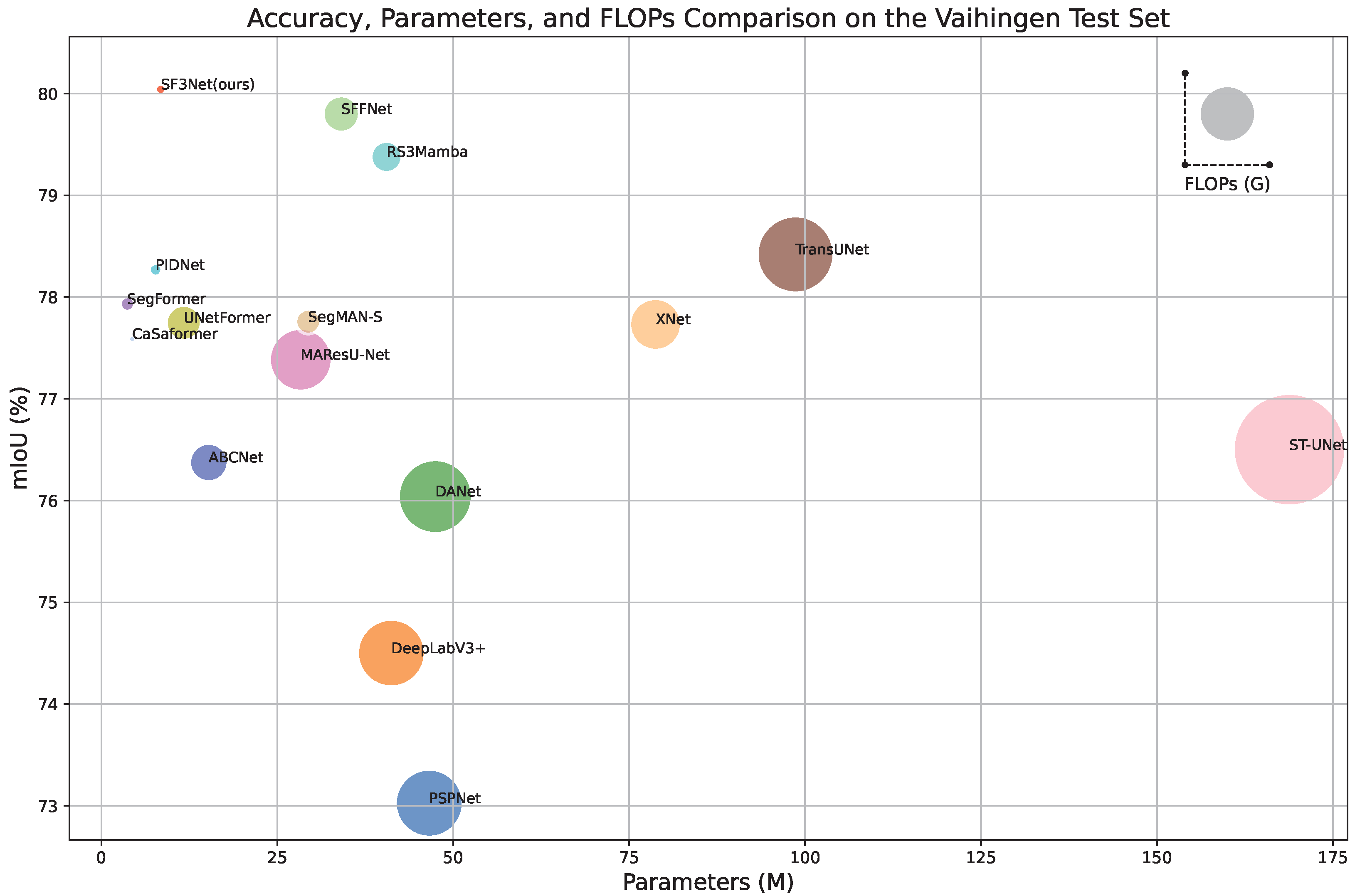
As depicted in Figure 1, SF3Net achieves a good balance between performance and model size. The contributions of this article are as follows.

Figure 1. Accuracy, Parameters and FLOPs comparison on the Vaihingen Test Set, the size of the circle represents FLOPs of network.

• A Frequency Feature Stereoscopic Learning (FFSL) module is proposed, in which adaptive frequency-domain weights are learned to suppress high-frequency noise and enhance informative spectral components through multi-dimensional Fourier modeling.
• A Spatial Feature Aggregation Module (SFAM) is designed to preserve structural details and aggregate spatial context, compensating for information loss during feature extraction.
• SF3Net is constructed, integrating spatial features from SFAM and frequency features from FFSL through a Spatial–Frequency Feature Fusion Module (SFFM). This unified framework jointly models spatial and frequency information, enhancing multi-scale perception and achieving more accurate and robust segmentation in complex RS imagery.

2. Methodology

In this section, we present the overall structure of the proposed SF3Net and subsequently introduce four important modules in SF3Net, namely, SFFM, FFSL, SFAM, and FSM.

2.1. Network Architecture

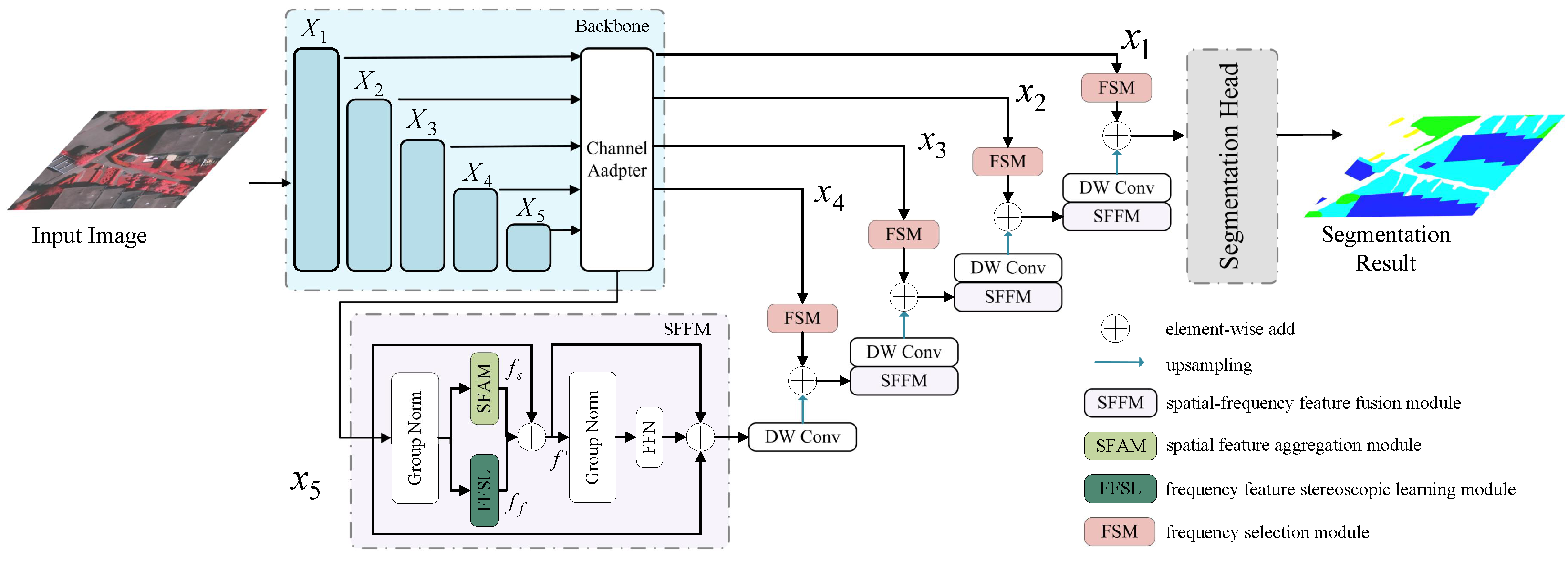
The structure of SF3Net is shown in Figure 2, designed as a U-shaped encoder–decoder architecture. In the encoding phase, MobileNetV2 [35] is used for comprehensive spatial feature extraction, with a channel adapter adjusting the number of channels to [16, 32, 48, 96, 128] to meet the decoder’s lightweight design requirements. In the decoding phase, SFFM is employed to perform frequency domain learning and spatial domain enhancement on the raw data with redundant information, followed by the fusion of the features processed from both representation domains. SFFM consists of two branches: the frequency domain feature stereoscopic learning branch and the spatial domain feature aggregation branch. The frequency domain feature stereoscopic learning branch utilizes Fast Fourier Transform (FFT) to map the raw features to frequency domain features, learning rich frequency domain information from three mutually perpendicular directions. The spatial domain feature aggregation branch uses two parallel dilated convolutions to expand the receptive field, followed by a series of average pooling, convolution, and activation operations to re-calibrate the feature channels. Finally, soft pooling is applied to aggregate pixel-level spatial information across two dimensional directions. Additionally, FSM is designed in the skip connection to adaptively select the shallow features from the encoder, compensating for the loss of detail information during the downsampling process.

Figure 2. The overall architecture of SF3Net. The main framework of the SF3Net encoder–decoder network consists of four key modules: FFSL, SFAM, SFFM, and FSM. During the decoding process, FFSL is first used for frequency domain feature mapping to obtain additional frequency information. Simultaneously, SFAM is employed to enhance spatial feature representation. Subsequently, SFFM is utilized to fuse the features from the two representation domains, ensuring the complementary nature of spatial and frequency domain features is maximized. Finally, FSM is utilized to compensate the detail loss during the encoder downsampling process.

Specifically, for an input image $\mathit{x}\in {\mathbb{R}}^{3\times h\times w}$, h and w represent the height and width of the input image, respectively. The encoding stage of feature extraction yields five features of different scales: $X_1\in {\mathbb{R}}^{16\times (H/2)\times (W/2)}$, $X_2\in {\mathbb{R}}^{32\times (H/4)\times (W/4)}$, $X_3\in {\mathbb{R}}^{96\times (H/8)\times (W/8)}$, $X_4\in {\mathbb{R}}^{320\times (H/16)\times (W/16)}$, $X_5\in {\mathbb{R}}^{1280\times (H/32)\times (W/32)}$, where H and W are the downsampled height and width. Then, the feature channels are adjusted to match the decoder using a channel adapter, consisting of a series of depthwise separable convolutions (DWConv), expressed as follows:

$$\begin{array}{c}\hfill {\mathit{x}}_i=DWConv\left(X_i\right)\end{array}$$

(1)

where i = 1, 2, 3, 4, 5, this stage yields five features of different scales after channel adapter: ${\mathit{x}}_1\in {\mathbb{R}}^{16\times (H/2)\times (W/2)}$, ${\mathit{x}}_2\in {\mathbb{R}}^{32\times (H/4)\times (W/4)}$, ${\mathit{x}}_3\in {\mathbb{R}}^{48\times (H/8)\times (W/8)}$, ${\mathit{x}}_4\in {\mathbb{R}}^{96\times (H/16)\times (W/16)}$, ${\mathit{x}}_5\in {\mathbb{R}}^{128\times (H/32)\times (W/32)}$.

Subsequently, ${\mathit{x}}_1$, ${\mathit{x}}_2$, ${\mathit{x}}_3$, ${\mathit{x}}_4$, ${\mathit{x}}_5$ are used as the raw data for the decoding stage. In decoding stage 5, after performing frequency domain feature stereoscopic learning and spatial domain feature aggregation on ${\mathit{x}}_5$, the features from both domains are fused to produce the output features $ou{t}_5$ of the SFFM.

Next, the output features $ou{t}_5$ obtained from the SFFM are upsampled and element-wise added to the most relevant shallow features selected adaptively by the FSM to form the input for the next stage of the decoder. Using this approach, the outputs of the five stages of the decoder are obtained: $ou{t}_5\in {\mathbb{R}}^{128\times (H/32)\times (W/32)}$, $ou{t}_4\in {\mathbb{R}}^{96\times (H/16)\times (W/16)}$, $ou{t}_3\in {\mathbb{R}}^{48\times (H/8)\times (W/8)}$, $ou{t}_2\in {\mathbb{R}}^{32\times (H/4)\times (W/4)}$, $ou{t}_1\in {\mathbb{R}}^{16\times (H/2)\times (W/2)}$. Finally, a segmentation head is used to generate the final pixel-level prediction.

2.2. Spatial–Frequency Feature Fusion Module

We designed the SFFM to efficiently incorporate frequency domain features with spatial features, as shown in Figure 2. The SFFM consists of two main branches: the spatial domain feature aggregation branch and the frequency domain feature stereoscopic learning branch. In first branch, SFAM is dedicated to spatial feature aggregation, enhancing spatial context information by using parallel dilated convolutions to expand the receptive field and applying soft pooling for pixel-level feature aggregation. Meanwhile, the FFSL branch performs frequency domain feature learning, where the original features are transformed into the frequency domain to capture detailed frequency characteristics. The outputs of two branches, $f_s$ and $f_f$, are then combined and passed through a Group Normalization layer. The resulting features, $f^{\prime }$, are processed further before being fed into a feed-forward network (FFN). This design allows the SFFM to efficiently combine both frequency and spatial domain features, leading to a more comprehensive feature representation for semantic segmentation task. The SFFM can be represented as follows:

$$\begin{array}{cc}\hfill f_s& =F_s\left(GroupNorm\left(x_{in}\right)\right)\hfill \\ \hfill f_f& =F_f\left(GroupNorm\left(x_{in}\right)\right)\hfill \\ \hfill f^{\prime }& =x_{in}\oplus f_s\oplus f_f\hfill \\ \hfill x_{out}& =x_{in}\oplus f^{\prime }\oplus FFN\left(GroupNorm\left(f^{\prime }\right)\right)\hfill \end{array}$$

(2)

where $F_s(·)$ and $F_f(·)$ denote the operations of the SFAM and FFSL for feature mapping, respectively, and ⊕ represents element-wise addition. $x_{in}$, $f_s$, $f_f$, $f^{\prime }$, and $x_{out}$ represent the input features, the mapped spatial features, frequency features, aggregation features, and the output features of SFFM, respectively.

2.3. Spatial Feature Aggregation Module

Although depthwise separable convolution effectively reduces memory consumption, it somewhat weakens the network’s ability to extract spatial structural information. Moreover, the loss of small-scale features caused by mutual occlusion of ground objects in RS images requires more precise spatial structural information to mitigate these challenges. To address this issue, we introduce the SFAM to encode spatial structural infomation more precisely, as shown in Figure 3. First, an dilated convolution with a dilation rate of 2 is applied to reduce the input channel size C to C/2, expanding the receptive field while reducing computational complexity. Then, the receptive field is further expanded using two parallel dilated convolutions with dilation rates of 1 and 3, respectively, and the results from both branches are concatenated for subsequent processing. Next, feature recalibration of the channel dimension is performed using average pooling, two continuous convolution and activation operations. By soft-pool [36] operation introducing attention mechanisms in both horizontal and vertical dimensions to account for pixel relationships, the SFAM overcomes the limitations of convolution operations in capturing global spatial structural information. Finally, a 1 × 1 convolution is used to adjust the number of channels C/2 back to C. This enhances the network’s ability to perceive spatial information in feature maps, thereby improving its representational capacity.

Figure 3. Structure of SFAM.

For an input feature $f_i$, the computation procedure can be expressed as follows:

$$\begin{array}{cc}\hfill f_i^{\prime }& =DCon{v}_{(3,2)}\left(f_i\right)\hfill \\ \hfill f_s^{\prime }& =Cat(DCon{v}_{(3,1)}\left(f_i^{\prime }\right),DCon{v}_{(3,3)}\left(f_i^{\prime }\right))\hfill \\ \hfill f_s^{″}& =f_s^{\prime }\odot \left(sigmoid\left(Conv\left(ReLU\left(Conv\left(Avgpool\left(f_s^{\prime }\right)\right)\right)\right)\right)\right)\hfill \\ \hfill v_{h_i}^k& ={\displaystyle \frac{{\sum }_{j=0}^{w-1}{\widehat{f_s^{″}}}^k(i,j)·e^{{\widehat{f_s^{″}}}^k(i,j)}}{{\sum }_{j=0}^{w-1}{e}^{{\widehat{f_s^{″}}}^k(i,j)}}}\hfill \\ \hfill v_{w_j}^k& ={\displaystyle \frac{{\sum }_{i=0}^{h-1}{\widehat{f_s^{″}}}^k(i,j)·e^{{\widehat{f_s^{″}}}^k(i,j)}}{{\sum }_{i=0}^{h-1}{e}^{{\widehat{f_s^{″}}}^k(i,j)}}}\hfill \\ \hfill f_s& =Conv(v_h\odot v_w)\hfill \end{array}$$

(3)

where i, j, and k represent the indexes for the vertical direction, horizontal direction, and the channel, respectively; $0\le i<h$, $0\le j<w$, $0\le k<c/2$, $DCon{v}_{(3,2)}$ denotes a dilation convolution with convolution kernel 3 and dilation rate 2; $Cat$ represents performing concatenation operation along the channel dimension; $Conv$ represents a 1 × 1 convolution operation; $f_i^{\prime }$, $f_s^{\prime }$ and $f_s^{″}$ denote the intermediate features of the computational process, respectively; and ⊙ stands for element-wise multiplication. The feature $\widehat{f_s^{″}}=f\left(f_s^{″}\right)$, where $f(·)$ represents a dilated convolution layer with Group Normalization and the GELU activation function. $v_h$ and $v_w$ capture the pixel-level weights of the feature map in the two spatial directions. By performing element-wise multiplication of $v_h$ and $v_w$ as shown in Equation (3), the position-aware output feature map $f_s$ is obtained.

2.4. Frequency Feature Stereoscopic Learning Module

In the field of RS image segmentation, recent methods have primarily focused on obtaining richer spatial domain information while often neglecting the significance of the frequency domain. In the spatial domain, the complex backgrounds of RS images frequently lead to blurred segmentation boundaries. In contrast, the frequency domain is more sensitive to grayscale variations, and different objects occupy distinct frequency domains, making them easier to differentiate [37]. Although prior work, such as [31,32,38], has introduced frequency domain features, the global information obtained remains insufficient and lacks effective integration with spatial features. Moreover, RS images are often affected by high-frequency noise caused by sensor limitations, atmospheric interference, and fine-scale clutter. This noise overlaps with true edges and details, making it difficult to distinguish informative from irrelevant frequency components and thus reducing segmentation robustness. To overcome these issues and enhance segmentation accuracy, we design the FFSL module.

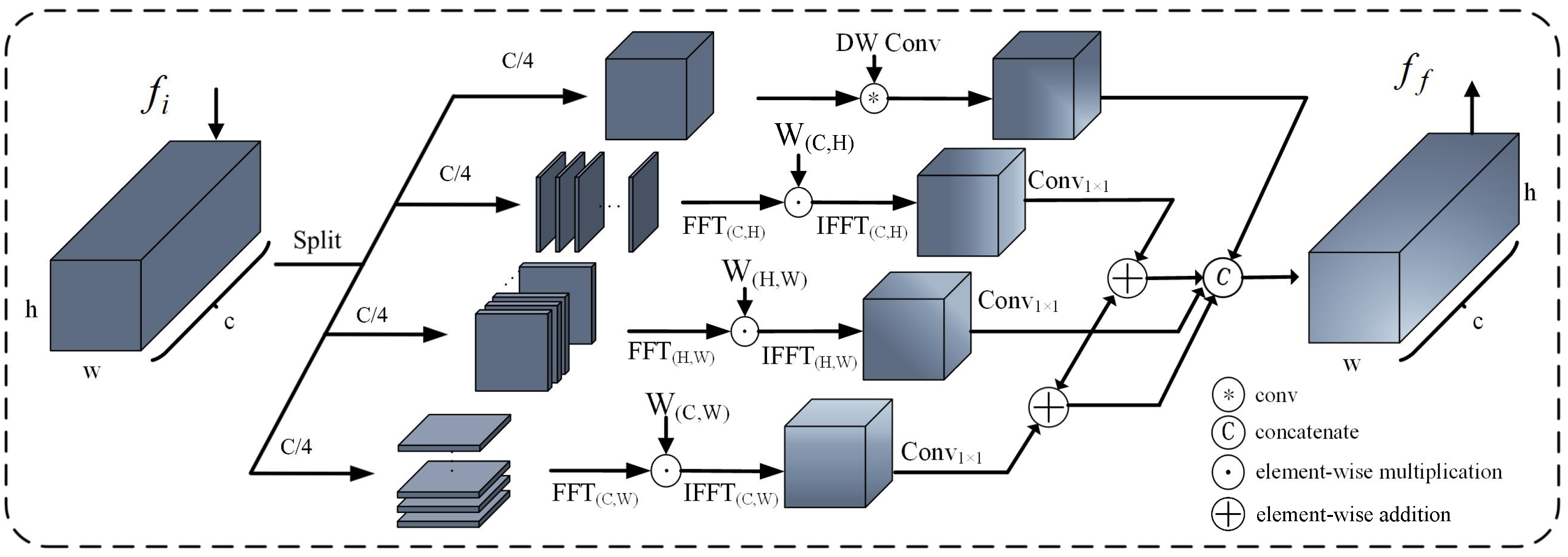
As shown in Figure 4, the input feature $f_i$ is split into four sub-features along the channel dimension, denoted as $f_{i1}$, $f_{i2}$, $f_{i3}$, and $f_{i4}$. Each sub-feature has the number of channels of the $f_i$ quarter. Depthwise separable convolution is then applied to $f_{i1}$ to compute the local spatial feature $f_{i1}^{\prime }$, ensuring that sufficient spatial information is retained for subsequent operations. The computation of $f_{i1}^{\prime }$ is defined as follows:

$$\begin{array}{cc}\hfill f_{i1},f_{i2},f_{i3},f_{i4}& =Split\left(f_i\right)\hfill \\ \hfill f_{i1}^{\prime }& =DWCon{v}_{3\times 3}\left(f_{i1}\right)\hfill \end{array}$$

(4)

where $\mathrm{Split}(·)$ denotes the splitting operation along the channel dimension.

Figure 4. Structure of FFSL.

We utilize the 2D fast fourier transform (FFT) to to extract frequency-domain features. The 2D FFT is an extension of the 1D FFT, applied across both spatial dimensions of an image. For each row x of the image $f(x,y)$, we compute the 1D FFT along the horizontal axis, then for each column v of the intermediate result $F(x,v)$, we compute the 1D FFT along the vertical axis. To derive the 2D FFT formulation, we substitute Equation (5) into Equation (6):

$$\begin{array}{cc}\hfill F(x,v)& =\sum _{y=0}^{N-1}f(x,y)·exp\left(-j2\pi {\displaystyle \frac{yv}{N}}\right)\hfill \end{array}$$

(5)

$$\begin{array}{cc}\hfill F(u,v)& =\sum _{x=0}^{M-1}F(x,v)·exp\left(-j2\pi {\displaystyle \frac{ux}{M}}\right)\hfill \end{array}$$

(6)

$$\begin{array}{cc}\hfill FFT(u,v)& =\sum _{x=0}^{M-1}\sum _{y=0}^{N-1}f(x,y)·exp\left(-j2\pi ({\displaystyle \frac{ux}{M}}+{\displaystyle \frac{yv}{M}})\right)\hfill \end{array}$$

(7)

where M and N are the dimensions of the image, $f(x,y)$ represents the pixel intensity at spatial coordinates $(x,y)$, $F(u,v)$ represents the frequency components at spatial frequencies $(u,v)$, and j is the imaginary unit.

Subsequently, 2D FFT operations are applied to $f_{i2}$, $f_{i3}$ and $f_{i4}$ to transform them into the frequency domain. Unlike a conventional 2D FFT applied solely on the spatial plane, these transforms are generalized to different dimension pairs of the feature tensor, i.e., “Channel-Height”, “Height-Width”, and “Channel-Width”. Three learnable weights, $W_{(C,H)}$, $W_{(H,W)}$ and $W_{(C,W)}$, each initialized with ones, serve as adaptive frequency filters that modulate the amplitude of different frequency components along their respective dimensions. Through task-driven backpropagation, these weights learn to attenuate noisy high-frequency signals while enhancing semantically meaningful low- and mid-frequency components. The computations are defined as follows:

$$\begin{array}{cc}\hfill FFT\left(f_{i2}\right)& =\sum _{c=0}^{(C/4)-1}\sum _{h=0}^{H-1}{f}_{i2}·exp\left(-j2\pi ({\displaystyle \frac{c{u}_c}{C/4}}+{\displaystyle \frac{h{v}_h}{H}})\right)\hfill \\ \hfill FFT\left(f_{i3}\right)& =\sum _{h=0}^{H-1}\sum _{w=0}^{W-1}{f}_{i3}·exp\left(-j2\pi ({\displaystyle \frac{h{u}_h}{H}}+{\displaystyle \frac{w{v}_w}{W}})\right)\hfill \\ \hfill FFT\left(f_{i4}\right)& =\sum _{c=0}^{(C/4)-1}\sum _{w=0}^{W-1}{f}_{i4}·exp\left(-j2\pi ({\displaystyle \frac{c{u}_c}{C/4}}+{\displaystyle \frac{w{v}_w}{W}})\right)\hfill \\ \hfill f_{i2(C,H)}& =W_{(C,H)}\odot FFT\left(f_{i2}\right)\hfill \\ \hfill f_{i3(H,W)}& =W_{(H,W)}\odot FFT\left(f_{i3}\right)\hfill \\ \hfill f_{i4(C,W)}& =W_{(C,W)}\odot FFT\left(f_{i4}\right)\hfill \end{array}$$

(8)

where ⊙ denotes the element-wise multiplication operation.

Next, the learned frequency domain feature $f_{i2(C,H)}$, $f_{i3(H,W)}$, and $f_{i4(C,W)}$ are transformed back into spatial-domain features $f_{i2}^{\prime }$, $f_{i3}^{\prime }$, and $f_{i4}^{\prime }$.

$$\begin{array}{cc}\hfill f_{i2}^{\prime }& =IFFT\left(f_{i2(C,H)}\right)\hfill \\ \hfill f_{i3}^{\prime }& =IFFT\left(f_{i3(H,W)}\right)\hfill \\ \hfill f_{i4}^{\prime }& =IFFT\left(f_{i4(C,W)}\right)\hfill \end{array}$$

(9)

where $\mathrm{IFFT}(·)$ denotes the inverse fast fourier transform.

The feature $f_{i2}^{\prime }$ and $f_{i3}^{\prime }$ are fused, and $f_{i4}^{\prime }$ and $f_{i3}^{\prime }$ are fused, resulting in global feature information enriched through frequency domain weight learning. Finally, the four parts are concatenated to produce the final output features of the FFSL module. This process can be denoted as follows:

$$\begin{array}{cc}\hfill f_{F_1}& =f_{i2}^{\prime }\oplus f_{i3}^{\prime }\hfill \\ \hfill f_{F_2}& =f_{i4}^{\prime }\oplus f_{i3}^{\prime }\hfill \\ \hfill f_f& =Cat(f_{i1}^{\prime },f_{F_1},f_{i3}^{\prime },f_{F_2})\hfill \end{array}$$

(10)

where $f_{F_1}$ and $f_{F_2}$ represent the fused features in the width-channel direction and the height-channel direction, respectively, and $f_f$ represents the output features from the FFSL.

2.5. Feature Selection Module

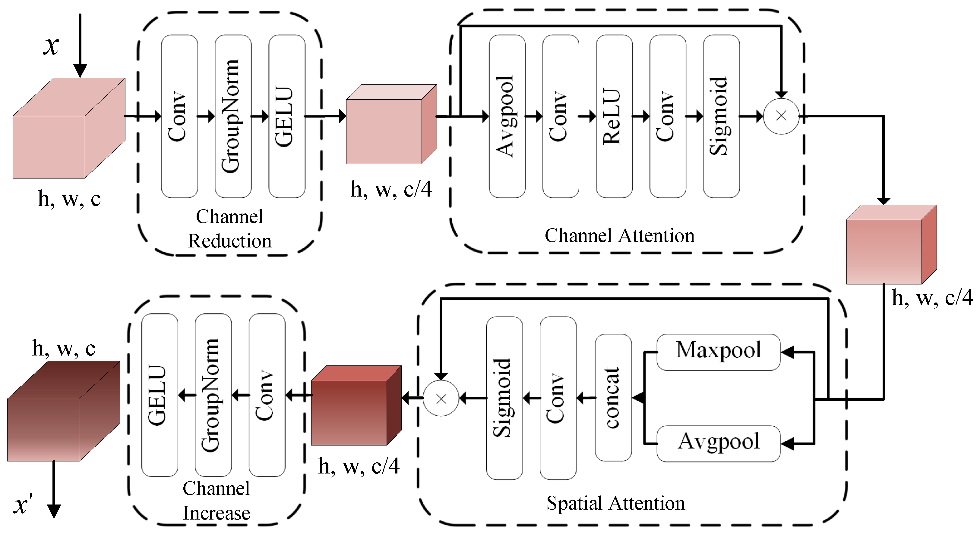
Although the skip connections in U-shaped networks partially compensate for the information loss during the encoder downsampling process, they also introduce noise from shallow features. To enable more refined selection and dynamic fusion of shallow features while reducing noise interference, we incorporate the FSM into the skip connections, as shown in Figure 5.

Figure 5. Structure of SFAM.

Specifically, for a feature from the encoder with size (h, w, c), the feature is first refined through convolution, GroupNorm, and GELU activation functions, reducing the channel dimension to (c/4)

$$\begin{array}{c}\hfill X^{\prime }=GELU\left(GroupNorm\left(Conv\left(x\right)\right)\right)\end{array}$$

(11)

where $X^{\prime }$ represents the features obtained through channel reduction operations.

Next, a channel attention module is applied to obtain the channel attention map, adjusting the importance of each channel and further emphasizing critical features

$$\begin{array}{cc}\hfill A_c& =Sigmoid\left(Conv\left(ReLU\left(Conv\left(Avgpool\left(X^{\prime }\right)\right)\right)\right)\right)\hfill \\ \hfill X_c& =A_c\otimes X^{\prime }\hfill \end{array}$$

(12)

Here, $A_c$ and $X_c$ represents the channel attention map and the features obtained through channel attention operations.

Subsequently, two operations, maximum pooling and average pooling in parallel combined with convolution and Sigmoid activation functions, are used to generate a spatial attention map, filtering the features in spatial dimensions and highlights the feature information in salient regions.

$$\begin{array}{cc}\hfill A_s& =Sigmoid\left(Conv\left(Cat(Maxpool\left(X_c\right),Avgpool\left(X_c\right))\right)\right)\hfill \\ \hfill X_s& =A_s\otimes X_c\hfill \end{array}$$

(13)

where $A_s$ and $X_s$ represents the spatial attention map and the features obtained through spatial attention operations.

Finally, a convolution operation is used to increase the channel dimension, restoring the feature to its original dimensionality.

$$\begin{array}{c}\hfill x^{\prime }=GELU\left(GroupNorm\left(Conv\left(X_s\right)\right)\right)\end{array}$$

(14)

Here, $x^{\prime }$ represents the features obtained through FSM. Through the processing of the FSM, the decoder’s performance in detail recovery and fine feature extraction is effectively enhanced, improving the overall performance of the network.

3. Dataset and Experimental Setting

3.1. Datasets

ISPRS-Vaihingen: The dataset contains 33 RS images with an average size of 2496 × 2064 pixels, covering a total area of 1.38 km² and a GSD of 9 cm. Following the methodology of previous studies [33,39,40], we use ground truth for testing. Specifically, 11 images (image numbers: 1, 3, 5, 7, 13, 17, 21, 23, 26, 32, and 37) are selected for training, image ID 30 is selected as the validation set, and 4 images (image numbers: 11, 15, 28, and 34) are used for testing.

ISPRS-Potsdam: This is a well-known dataset provided for the 2-D labeling competition, consisting of 38 RS images, each with a size of 6000 × 6000 pixels and a GSD of up to 5 cm. Following the methodology of previous studies [33,39,40], 22 images (image numbers: 2_11, 2_12, 3_10, 3_11, 3_12, 4_10, 4_11, 4_12, 5_10, 5_11, 5_12, 6_07, 6_08, 6_09, 6_10, 6_11, 6_12, 7_07, 7_08, 7_09, 7_11, and 7_12) are used for training, ID 2_10 is selected as the validation set, and the remaining 15 images are used for testing.

The Vaihingen and potsdam datasets include the following land cover classes: Impervious Surface, Building, Low Vegetation, Tree, Car, and Clutter/background. Each image is cropped into 512 × 512 patches.

Farmland: Using the DJI Phantom 4 RTK drone, three high-resolution images were captured and stitched together near Dapo Township, Qujing City, Yunnan Province, China. The resolutions of the images are 43,141 × 42,489, 22,866 × 27,463, and 14,452 × 12,638, respectively. The original images were annotated using Labelme, and then cropped with a 12-pixel overlap using ENVI (version 5.3), resulting in patches of 512 × 512. Due to the irregular shape of the captured region, pixel padding was applied during the stitching process, and images with irrelevant pixels occupying more than 75% of the total pixels were removed. Finally, the remaining image data was divided and processed into a five-class Farmland dataset (Tobacco 1, Tobacco 2, Tobacco 3, Other Farmland, and Background). The dataset contains 7264 images, randomly divided into a training set (5811), a validation set (726), and a test set (727) in an 8:1:1 ratio. This dataset can be obtained from https://github.com/Yihe502/SF3Net and accessed on 15 November 2025.

Figure 6 shows the proportion of each semantic label in the three datasets mentioned above. Following [33,39,40,41], we conducted experiments on the ISPRS-Vaihingen and ISPRS-Potsdam datasets, ignoring the clutter/background class.

Figure 6. The proportion of semantic labels for each class in the Potsdam, Vaihingen, and Farmland datasets.

3.2. Implementation Details

All experiments were conducted on a computer equipped with a single NVIDIA RTX 4090D GPU, using PyTorch 2.0.0 framework.

1.

Data Preprocessing: During the training phase, we introduced multiple data augmentation techniques, including random scaling (0.5, 0.75, 1.0, 1.25, 1.5), random flipping, and random ratation. During the testing phase, we employed multiscale evaluation and random flipping augmentation techniques to ensure the robustness and performance of the models.

2.

Training Settings: We use AdamW as the optimizer, setting the weight decay to 0.05, ${\beta }_1$ = 0.9, ${\beta }_2$ = 0.999, initial learning rate to $1.2\times {10}^{-4}$. In addition, we adopt the “poly” learning rate decay strategy and the model is trained using the joint loss function of cross-entropy and dice.

$$\begin{array}{cc}\hfill L_{CE}& =-{\displaystyle \frac{1}{M}}\sum _{m=1}^M\sum _{k=1}^K{y}_k^{\left(m\right)}log{\widehat{y}}_k^{\left(m\right)}\hfill \end{array}$$

(15)

$$\begin{array}{cc}\hfill L_{Dice}& =1-{\displaystyle \frac{2}{M}}\sum _{m=1}^M\sum _{k=1}^K{\displaystyle \frac{y_k^{\left(m\right)}{\widehat{y}}_k^{\left(m\right)}}{y_k^{\left(m\right)}+{\widehat{y}}_k^{\left(m\right)}}}\hfill \end{array}$$

(16)

$$\begin{array}{cc}\hfill L& =L_{CE}+L_{Dice}\hfill \end{array}$$

(17)

where M represents the number of training samples, and K denotes the number of categories in the dataset. $y_k^{\left(m\right)}$ and ${\widehat{y}}_k^{\left(m\right)}$ represent the ground truth semantic labels and the confidence of sample m belonging to category k, respectively. During the training process, we set the batch size to 4 and the maximum iter to 80 K.

3.3. Evaluation Metrics

In our experiments, we adopted commonly used metrics in remote sensing segmentation: The first focuses on segmentation accuracy, utilizing mean intersection over union (mIoU) and Average F1-score (AF1). The second emphasizes the model’s memory requirements and computational speed, measured by the parameters and FLOPs metrics. The calculation methods are as follows:

$$\begin{array}{cc}\hfill \mathrm{IoU}& ={\displaystyle \frac{\mathrm{TP}}{\mathrm{TP}+\mathrm{FN}+\mathrm{FP}}}\hfill \end{array}$$

(18)

$$\begin{array}{cc}\hfill \mathrm{Precision}& ={\displaystyle \frac{\mathrm{TP}}{\mathrm{TP}+\mathrm{FP}}}\hfill \end{array}$$

(19)

$$\begin{array}{cc}\hfill \mathrm{Recall}& ={\displaystyle \frac{\mathrm{TP}}{\mathrm{TP}+\mathrm{FN}}}\hfill \end{array}$$

(20)

$$\begin{array}{cc}\hfill \mathrm{F}1& ={\displaystyle \frac{2\times \mathrm{Precision}\times \mathrm{Recall}}{\mathrm{Precision}+\mathrm{Recall}}}\hfill \end{array}$$

(21)

where TP, FP and FN represent the counts of true positives, false positives and false negatives, respectively, each corresponding to specific classes of objects.

4. Experimental Results and Analysis

4.1. Ablation Experiments

To assess the effectiveness of our proposed SF3Net, we conducted a series of ablation experiments validated on the Vaihingen dataset. All experiments’ results are reported as the average of multiple trials. Furthermore, we investigated the impact of the backbone on the proposed network.

4.1.1. Influence of Frequency Fomain Feature Stereoscopic Learning Module

As shown in Table 1, incorporating the FFSL module into the Baseline improves mIoU by 1.165% and AF1 by 0.735%. The data presented in Table 2 clearly demonstrates that employing depthwise separable convolutions to preserve local information has a significant positive impact on enhancing the overall segmentation performance of the model. Concurrently, extracting frequency-domain features from three dimensions (C-H, H-W, and C-W) compared to single-direction or two-direction combinations, enables the acquisition of richer and more comprehensive frequency-domain features, thereby significantly enhancing the model’s overall segmentation capability. Experimental results demonstrate that the mIoU metric improved by at least 0.574%, while the AF1 metric increased by at least 0.469%. The visualization results in Figure 7 further demonstrate that adding frequency domain features to the Baseline enhances segmentation performance, particularly in edge regions and areas with significant shadow variations. By leveraging frequency domain features through the FFSL, the model’s segmentation capability in regions with substantial grayscale variations is greatly improved.

Table 1. Ablation experiment of the proposed modules on the Vaihingen dataset.

Method	mIoU (%)	AF1 (%)	Parameters (M)	FLOPs (G)
Baseline	77.598	87.214	2.156	2.051
Baseline + FFSL	78.763 (↑ 1.165)	87.949 (↑ 0.735)	7.870	3.680
Baseline + SFAM	78.409 (↑ 0.811)	87.563 (↑ 0.349)	7.014	3.416
Baseline + FFSL + SFAM	78.812 (↑ 1.214)	88.085 (↑ 0.871)	7.945	3.719
Baseline + SFFM	79.034 (↑ 1.436)	88.378 (↑ 1.164)	8.046	3.834
Baseline + FSM	78.379 (↑ 0.781)	87.391 (↑ 0.177)	2.378	2.894
Baseline + FSM + SFFM	80.040 (↑ 2.442)	88.807 (↑ 1.593)	8.454	4.056

The (↑) represents an improvement in performance.

Table 2. Ablation experiment for the FFSL module on the Vaihingen dataset.

DWConv	W (C,W)	W (H,W)	W (C,H)	mIoU (%)	AF1 (%)
−	−	−	−	78.409	87.563
√				78.638	87.676
√	√			78.812	87.914
√		√		78.742	87.762
√			√	78.988	88.048
√	√	√		79.360	88.262
√	√		√	79.466	88.338
√		√	√	79.260	88.206
√	√	√	√	80.040	88.807

The (−) and (√) represent the removal operation and the addition operation respectively.

Figure 7. Comparison of the baseline before and after using the FFSL. (a) Baseline and (b) Baseline + FFSL.

4.1.2. Influence of Spatial Feature Aggregation Module

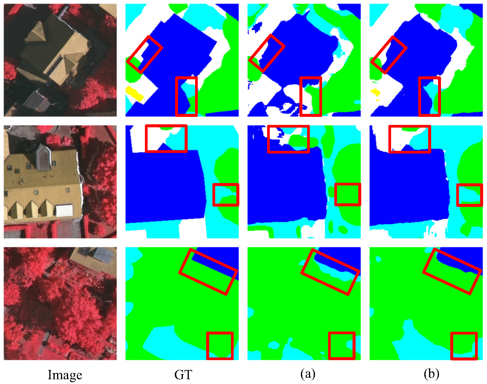
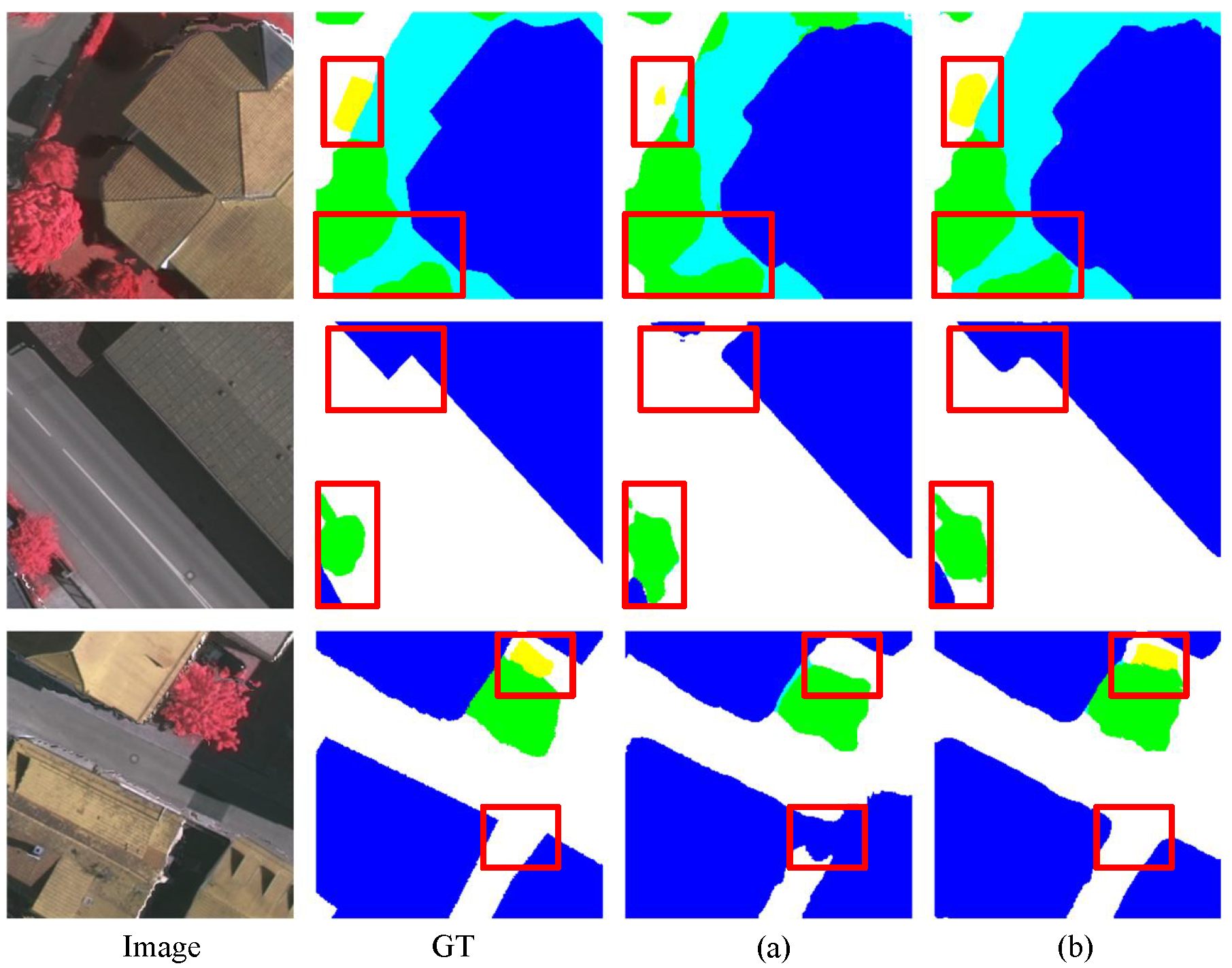
As shown in Table 1, incorporating the SFAM increases mIoU by 0.811% and AF1 by 0.349% compared to the Baseline. More intuitively, the comparison of the visual segmentation results is shown in Figure 8. In the first and second rows, the segmentation results of the model with SFAM are significantly clearer than those of the Baseline, particularly in handling the “Car” category when occluded by “Tree”, where the performance is notably superior. In the third row, the “Car” located next to the “Building” is missed by the Baseline but is accurately identified by the model with SFAM. These results highlight that incorporating SFAM preserves more detail and spatial structure information, significantly enhancing segmentation accuracy.

Figure 8. Comparison of the baseline before and after using the SFAM. (a) Baseline and (b) Baseline + SFAM.

4.1.3. Influence of Spatial–Frequency Feature Fusion Module

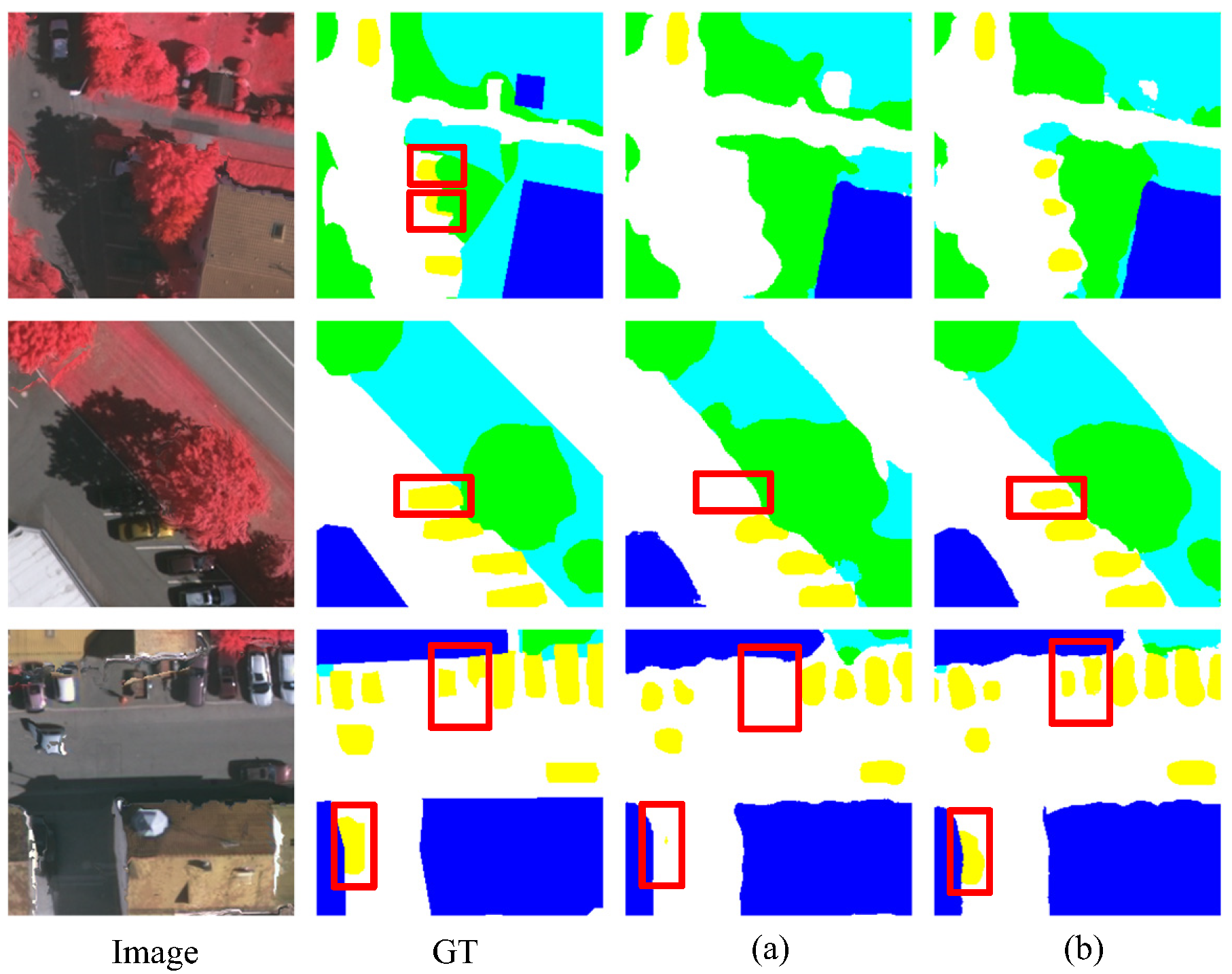
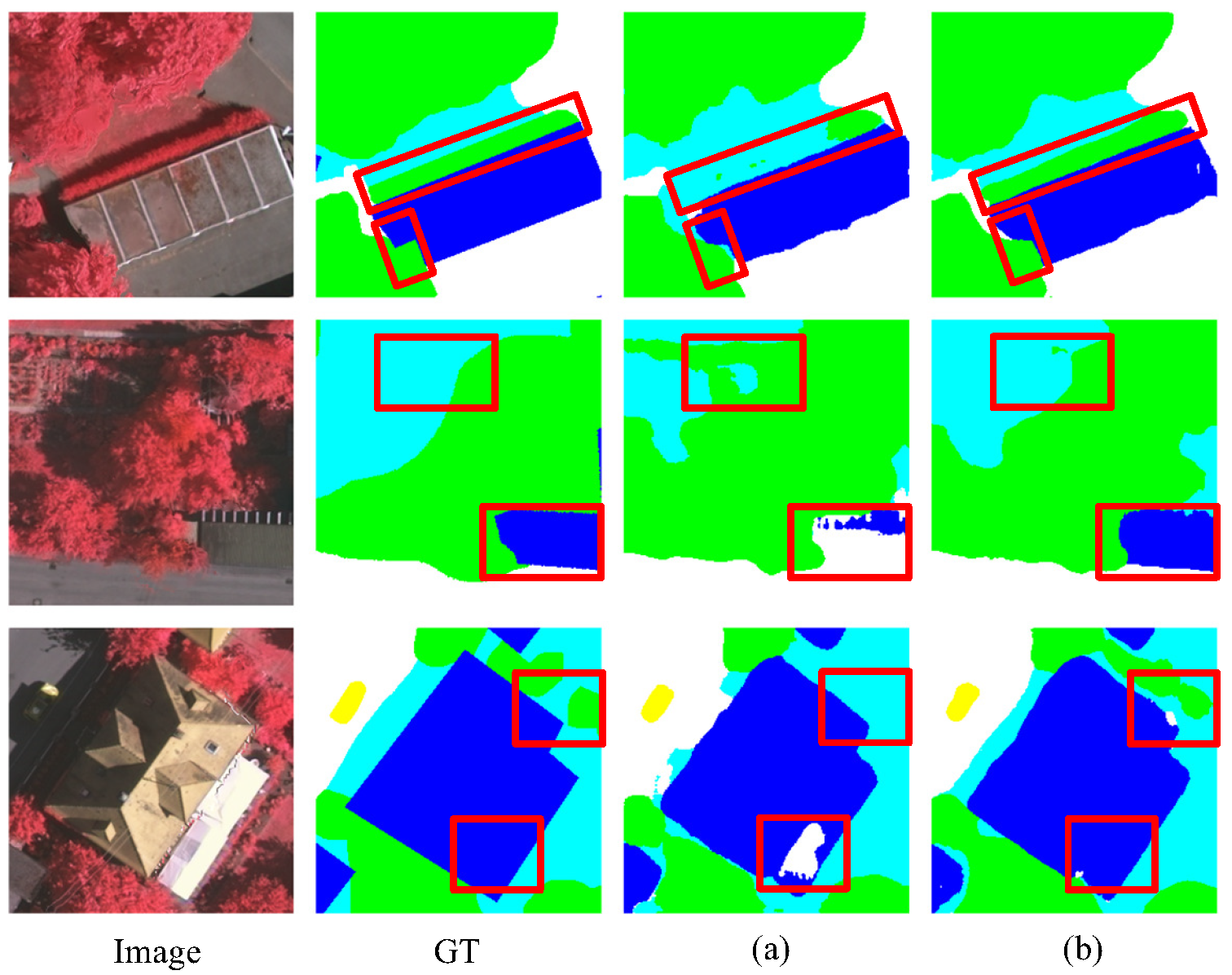
As shown in Table 1, SFFM improves mIoU by 1.436% and AF1 scores by 1.164% by integrating the additional frequency domain information introduced by FFSL and the enhanced spatial structural information from SFAM. Furthermore, compared to the directly concatenated FFSL and SFFM, the SFFM achieves a 0.22% improvement in mIoU and a 0.522% improvement in AF1, with only a marginal increase of 0.101 M parameters and 0.115 G FLOPs. As shown in Figure 9, in the first and third rows, the Baseline fails to effectively identify the “car” under shadow occlusion and the region with significant features. But the model correctly identifies these objects after adding SFFM. Furthermore, in the second row, the inclusion of SFFM improves the Baseline’s ability to handle details, such as the “Building” and “Tree” categories. These results demonstrate the effectiveness of SFFM in integrating frequency domain and spatial domain features. It preserves the detail information of spatial domain features while enhancing the model’s segmentation ability in regions with significant edge and texture changes through the introduction of frequency domain features.

Figure 9. Comparison of the baseline before and after using the SFFM. (a) Baseline and (b) Baseline + SFFM.

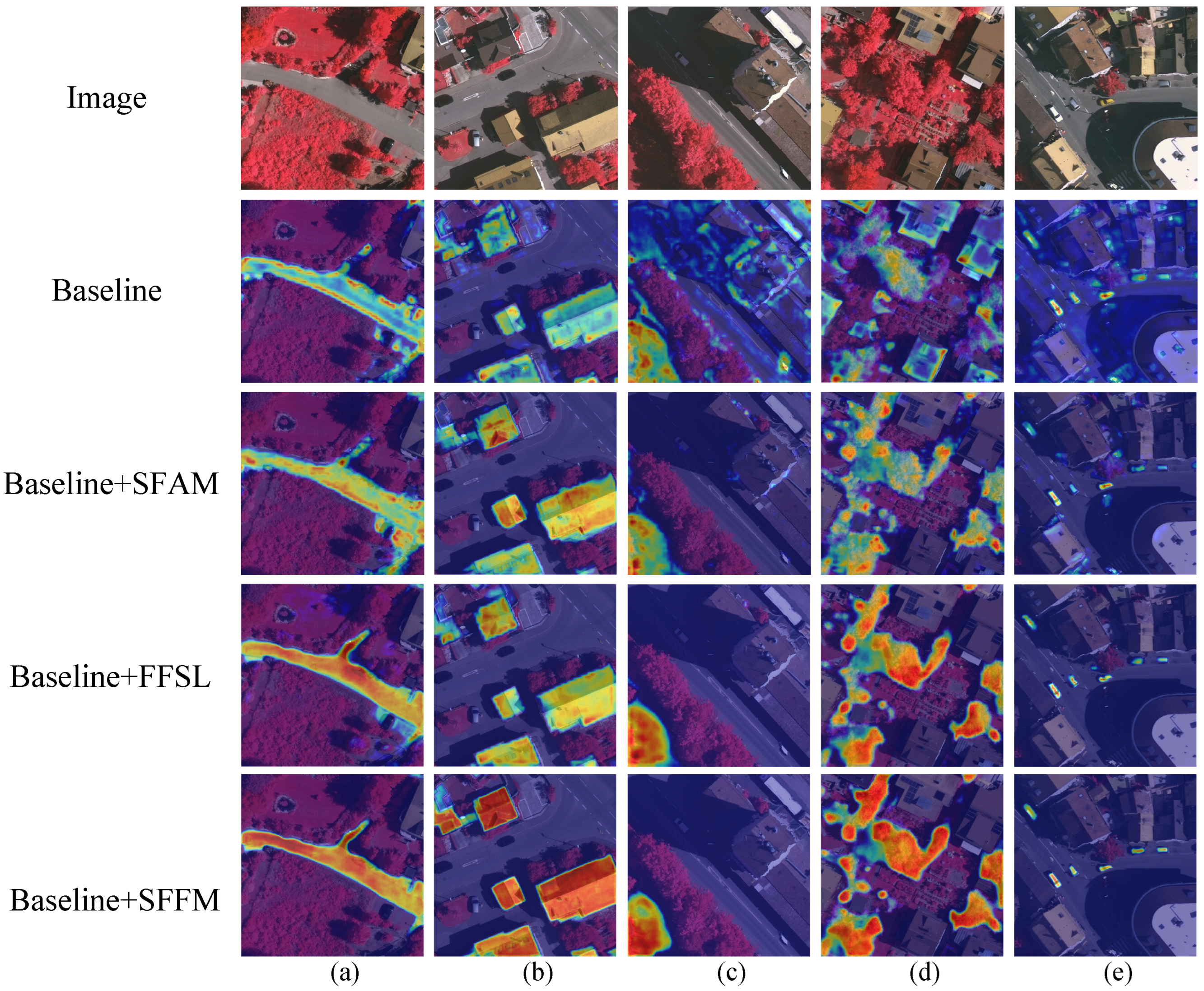
We also visualized the feature heatmaps of the last layer of the Baseline model decoder before and after adding SFAM, FFSL and SFFM to each category, as shown in Figure 10. Starting from the baseline model (second row), the progressive introduction of the SFAM (third row), FFSL (fourth row), and finally the SFFM (fifth row) clearly validates the effectiveness of each component through this incremental enhancement approach. In terms of edge segmentation, compared to the blurred edge activations of the baseline model, the SFFM generates sharp and precise boundary responses. In the boundary regions between “impervious surfaces” and “low vegetation” (columns a and c), improved edge preservation capabilities and reduced feature leakage phenomena are evident. When handling imbalanced classes, the improvement for “Car” (column e) is particularly pronounced, where the baseline model exhibits weak activation capabilities for small targets, while the SFFM produces concentrated and high-intensity responses at vehicle locations, significantly enhancing small target detection performance. “Tree” regions (column d) demonstrate better feature continuity and completeness. The visualization results indicate that the SFAM primarily enhances intra-target consistency, the FFSL strengthens edge and detail representation, while the SFFM perfectly combines the advantages of both, achieving optimal balance between boundary precision and target completeness. This provides robust and accurate feature representation for semantic segmentation of remote sensing images.

Figure 10. Visualization of heatmap on the Vaihingen dataset for SFAM, FFSL, and SFFM integrated into the baseline model. (a) Impervious surface. (b) Building. (c) Low vegetation. (d) Tree. (e) Car.

4.1.4. Influence of Feature Selection Module

As shown in Table 1, incorporating FSM improves mIoU and AF1 scores by 0.781% and 0.177%, respectively. The visualization results in Figure 11 demonstrate significant improvements in the segmentation of edge and detail. In the first and third rows, compared to the Baseline, the segmentation accuracy of continuous edge regions is noticeably improved, particularly for the “Tree” and “Low Vegetation” categories. In the second row, the segmentation accuracy of the “Building” category is also enhanced. These results highlight the effectiveness of using FSM in skip connections to reduce noise propagation and dynamically fuse shallow features, leading to more accurate segmentation.

Figure 11. Comparison of the baseline before and after using the FSM: (a) Baseline and (b) Baseline + FSM.

4.1.5. Influence of Different Backbone Networks

The choice of backbone network significantly affects performance. To analyze this, we conducted a series of backbone replacement experiments on the Vaihingen dataset, using several common and widely adopted backbone models, including ResNet50, ResNext50, MobileNetV2, MobileNetV3-small, and ConvNext-Tiny. The experimental results are shown in Table 3. From the data in Table 3, it is evident that although ResNet50 achieves the highest accuracy, its parameter count is nearly four times larger than MobileNetV2. However, when using MobileNetV3-small, the backbone with the fewest parameters, the accuracy is the lowest. Therefore, we prefer to use MobileNetV2 as the backbone model due to its balance of high accuracy and low parameter count.

Table 3. Number of parameters for differnet backbones on the Vaihingen dataset’s mIoU. The (↑) represents an improvement in performance.

Method	Backbone	Parameters (M) ↓	mIoU (%) ↑
	ResNet50	29.953	80.386
	ResNext50	29.422	80.144
SF3Net	MobileNetV2	8.454	80.040
	MobileNetV3-small	7.048	77.744
	ConvNext-Tiny	19.721	78.824

The (↓) and (↑) represent performance degradation and performance improvement, respectively.

4.2. Comparative Experiments

To validate the efficacy of our proposed SF3Net, a comprehensive analysis is performed comparing it with various advanced segmentation models, namely, PSPNet [42], DeepLabV3+ [14], DANet [13], ABCNet [43], SegFormer [26], TransUNet [44], MAResU-Net [45], ST-UNet [40], UNetFormer [46], PIDNet [47], CaSaFormer [48], XNet [31], SFFNet [33], RS3Mamba [29] and SegMAN [49]. For fairness of comparison, these models adopt ResNet-50 as the backbone. In addition, unless otherwise specified, all quantitative experimental results are presented as percentages (%). The precision results on the three datasets are presented in Table 4, Table 5 and Table 6.

Table 4. Comparison of segmentation results on the Vaihingen test set.

Method	Imp. Surf.	Building	Low Veg.	Tree	Car	mIoU	AF1
PSPNet	78.325/87.277	81.173/89.384	63.961/79.639	76.020/86.213	65.651/79.049	73.026	84.312
DeepLabV3+	79.362/88.649	84.341/89.562	64.657/80.031	76.512/86.331	67.631/80.483	74.501	85.011
DANet	80.738/90.397	85.661/90.253	66.567/80.346	77.734/86.871	69.496/80.838	76.039	85.941
ABCNet	81.883/91.209	84.791/90.013	66.899/80.761	77.981/86.915	70.314/81.537	76.374	86.287
SegFormer	84.061/91.943	88.730/93.702	69.082/82.411	81.389/89.740	66.397/79.809	77.932	87.521
TransUNet	82.361/90.333	87.639/93.410	68.070/81.000	80.593/89.249	73.432/83.000	78.419	87.398
MAResU-Net	82.172/91.995	86.497/90.760	67.920/81.152	78.477/87.856	71.854/82.086	77.384	86.770
ST-UNet	81.381/90.882	86.780/91.021	67.011/80.884	76.993/86.453	70.337/81.603	76.500	86.169
UNetFormer	82.845/92.055	86.864/92.970	67.936/81.769	78.967/88.316	72.124/82.503	77.747	87.523
PIDNet	83.215/92.332	89.930/94.137	68.284/81.872	79.839/88.400	70.065/81.400	78.267	87.628
CaSaFormer	83.411/92.553	88.450/93.396	67.279/80.443	79.858/88.800	68.942/80.747	77.588	87.188
XNet	81.697/91.039	89.378/93.860	67.422/80.939	80.177/89.134	69.981/81.257	77.731	87.246
SFFNet	83.791/92.437	90.759/94.021	68.994/82.189	81.875/90.614	73.578/82.978	79.799	88.448
RS3Mamba	84.187/92.424	89.973/94.072	68.679/81.433	79.964/88.869	74.083/84.110	79.377	88.182
SegMAN-S	83.438/91.962	88.660/93.989	69.648/82.810	78.630/88.039	68.413/80.968	77.758	87.554
SF3Net(Ours)	84.207/92.831	91.433/95.239	69.857/83.150	80.840/89.416	73.864/83.400	80.040	88.807

The (red) and (green) represent the best and second-best performance, respectively.

Table 5. Comparison of segmentation results on the Potsdam test set.

Method	Imp. Surf.	Building	Low Veg.	Tree	Car	mIoU	AF1
PSPNet	80.858/89.995	86.536/91.359	69.961/81.024	72.031/83.174	75.875/83.992	77.052	85.909
DeepLabV3+	82.174/91.426	87.781/93.812	70.356/81.740	72.382/83.883	78.587/86.672	78.256	87.507
DANet	82.741/91.563	87.192/93.326	71.427/82.387	73.640/84.055	79.627/86.437	78.925	87.554
ABCNet	82.053/91.025	87.763/93.957	72.974/83.870	73.834/84.000	80.114/87.763	79.348	88.123
SegFormer	84.458/91.580	88.831/94.082	73.753/84.899	75.354/85.940	87.281/93.208	81.935	89.942
TransUNet	82.240/91.251	87.931/94.672	71.439/83.337	76.164/86.469	87.670/93.433	81.089	89.832
MAResU-Net	82.975/91.756	90.112/94.833	74.798/84.191	75.118/84.565	82.783/90.164	81.157	89.102
ST-UNet	82.637/91.550	87.673/93.543	72.291/83.034	73.770/84.271	81.377/89.575	79.550	88.395
UNetFormer	83.249/92.075	90.504/94.930	74.216/84.536	75.649/84.831	84.416/91.371	81.607	89.549
PIDNet	84.513/92.664	90.835/95.049	74.325/84.770	75.317/85.024	86.642/91.963	82.326	89.894
CaSaFormer	84.442/92.578	89.879/94.678	73.875/84.094	76.578/86.731	87.369/93.700	82.429	90.356
XNet	83.713/92.264	89.801/93.890	73.051/83.933	73.009/84.327	81.895/90.034	80.294	88.890
SFFNet	85.705/93.253	90.726/94.997	76.940/86.637	77.763/86.731	87.141/92.543	83.655	90.832
RS3Mamba	85.591/93.243	90.808/95.181	73.527/83.975	77.450/87.294	89.329/94.353	83.341	90.809
SegMAN-S	83.058/92.741	89.600/94.039	74.729/84.452	76.912/86.645	85.081/91.943	81.876	89.964
SF3Net(Ours)	86.008/93.681	91.674/95.649	75.168/85.818	78.182/87.752	88.637/93.980	83.934	91.376

The (red) and (green) represent the best and second-best performance, respectively.

Table 6. Comparison of segmentation results on the Farmland test set.

Method	Background	Other Land	Tobacco 1	Tobacco 2	Tobacco 3	mIoU	AF1
PSPNet	87.623/90.434	91.156/93.923	60.268/72.383	87.364/90.275	88.932/91.981	83.069	87.799
DeepLabV3+	89.012/91.880	92.414/94.659	62.571/74.134	88.314/91.414	89.975/93.013	84.457	89.020
DANet	90.413/92.577	93.467/95.503	64.378/77.350	89.417/92.801	90.899/94.304	85.715	90.507
ABCNet	90.674/92.970	93.791/95.904	64.978/77.790	89.143/92.392	91.241/94.921	85.965	90.795
SegFormer	90.763/95.160	96.769/98.363	68.241/81.118	90.019/94.753	94.270/97.054	88.012	93.290
TransUNet	89.921/94.694	96.540/98.240	64.624/77.709	88.912/92.450	92.533/96.116	86.506	91.842
MAResU-Net	90.789/94.913	95.437/97.457	67.015/79.578	89.654/93.852	94.789/97.242	87.537	92.608
ST-UNet	89.868/92.091	93.589/95.734	64.621/77.868	89.523/93.136	91.419/95.278	85.804	90.821
UNetFormer	91.003/95.217	95.779/97.813	67.341/80.143	90.913/94.512	94.687/97.519	87.945	93.041
PIDNet	91.308/95.638	95.489/97.848	67.349/80.278	91.348/95.239	94.411/97.023	87.981	93.205
CaSaFormer	90.754/94.837	96.346/98.039	66.437/79.830	91.086/94.766	93.930/96.869	87.711	92.868
XNet	88.865/91.214	93.531/95.841	65.668/78.419	88.817/92.318	91.783/95.177	85.733	90.594
SFFNet	91.634/95.734	95.156/97.317	67.734/80.579	91.339/95.173	94.637/97.623	88.100	93.285
RS3Mamba	92.212/95.948	97.031/98.488	70.192/82.514	92.893/96.321	94.138/96.980	89.293	94.050
SegMAN-S	91.372/95.540	96.621/98.330	68.273/81.139	91.498/95.641	94.320/97.080	88.417	93.546
SF3Net(Ours)	91.433/95.521	96.856/98.410	68.341/81.193	91.724/95.680	94.931/97.980	88.657	93.757

The (red) and (green) represent the best and second-best performance, respectively.

4.2.1. Experimental Results on the Vaihingen Dataset

Table 4 presents the numerical results for each model on the Vaihingen dataset. The results show that our SF3Net achieves performance metrics of 80.040% for mIoU and 88.807% for AF1, respectively. DeepLabV3+ utilizes ASPP to expand the receptive field and capture multi-scale information, achieving better performance than PSPNet. while DANet leverages a dual attention mechanism to extract richer global context from both spatial and channel dimensions, delivering promising results. Compared to other networks, SF3Net performs best in terms of mIoU and AF1, outperforming the pure convolutional network ABCNet, MAResU-Net and PIDNet. Additionally, Transformer-based methods, SegFormer, TransUNet, UNetFormer, ST-UNet, and CaSaFormer, show a strong segmentation ability. In addition to the spatial domain-based methods mentioned above, SFFNet leverages wavelet transform for spatial–frequency fusion, achieving suboptimal accuracy, especially superior to XNet. Compared to SFFNet, SF3Net improves mIoU by 0.241%, AF1 by 0.359%, respectively. Furthermore, compared with the Mamba-based RS3Mamba and SegMAN, SF3Net achieves increases in mIoU of 0.663% and 2.282%, respectively, and improvements in AF1 of 0.625% and 1.253%, respectively.

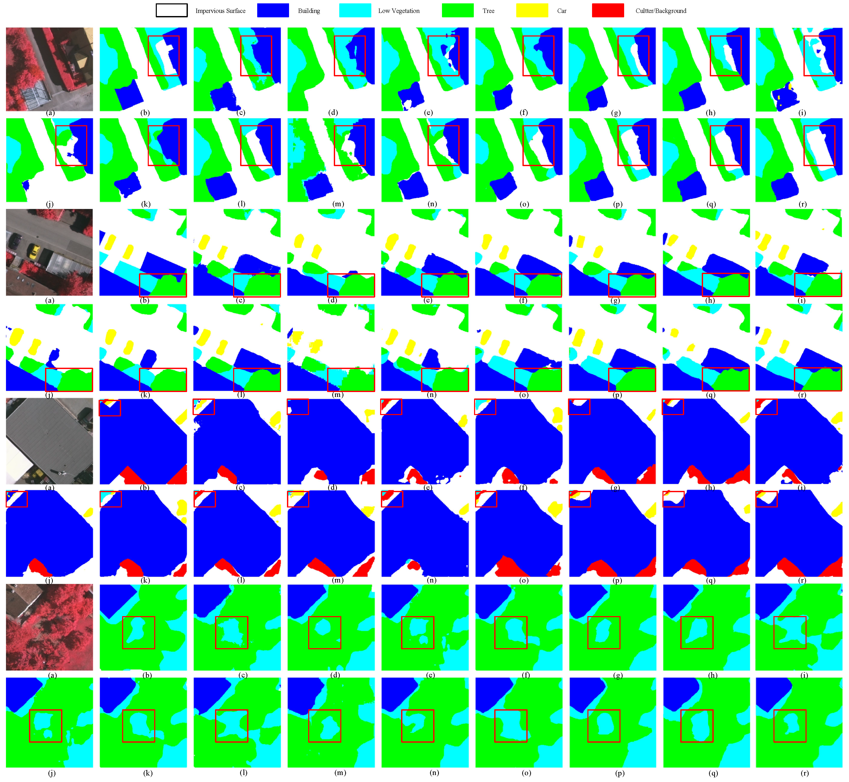
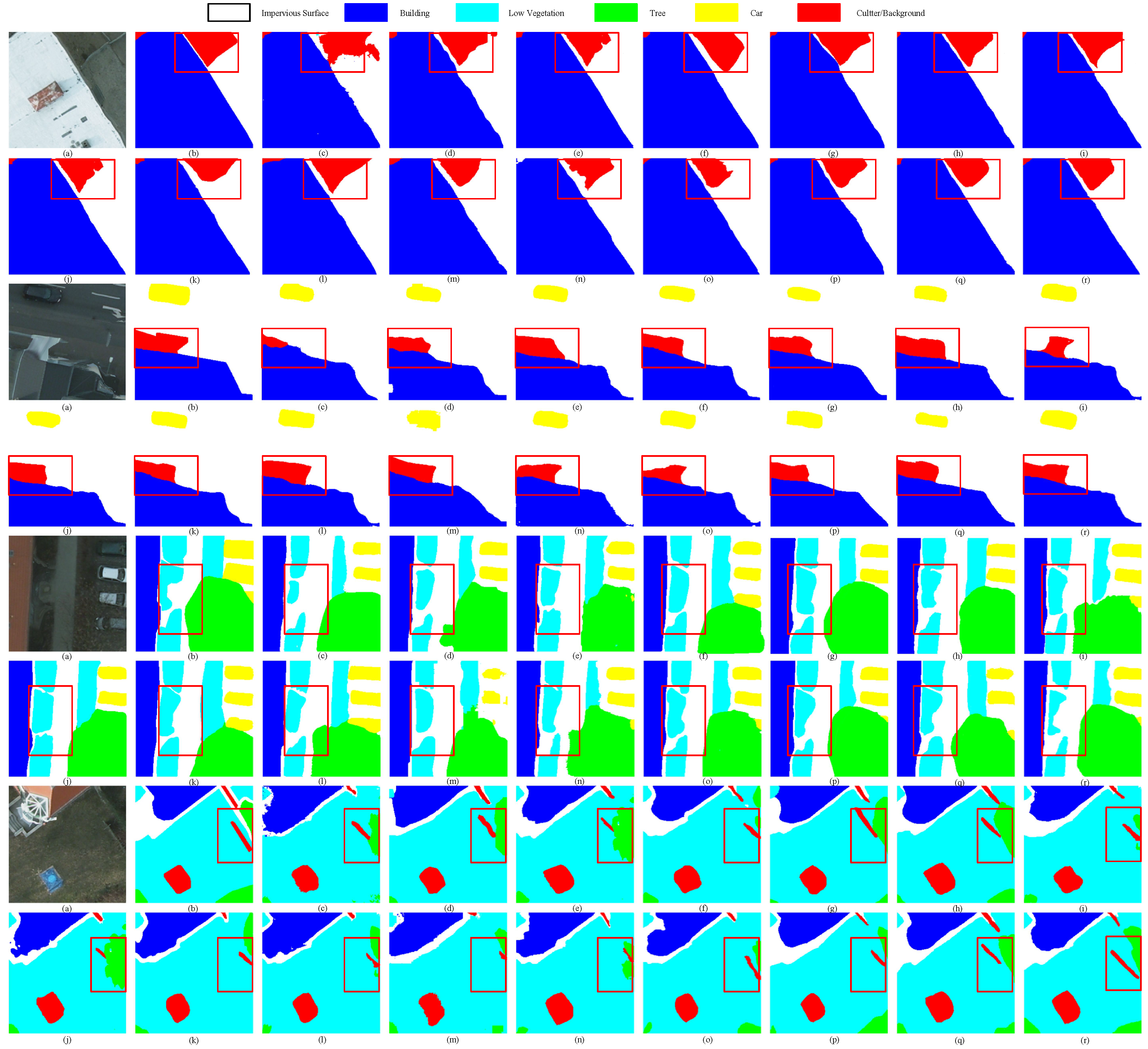
As shown in the second and eighth rows of Figure 12, methods with global modeling capabilities, such as ST-UNet, SFFNet, RS3Mamba, SegMAN and SF3Net, achieve better segmentation results in terms of continuity and correlation of large-scale features compared to CNN-based models like PSPNet and DANet. Furthermore, as observed in the fourth and eighth rows of Figure 12, methods such as ST-UNet and SF3Net, which incorporate spatial feature interaction, demonstrate better performance in mitigating poor segmentation results caused by occlusion. Furthermore, as shown in the first, second, third, and fourth rows of Figure 12, compared to purely spatial segmentation methods (e.g., DeepLabV3 and PIDNet), models incorporating frequency domain features, such as SFFNet and SF3Net, achieve superior segmentation results in shadowed regions (first and third rows), areas with significant texture variations (seventh row) and edges (fifth and sixth rows). However, as shown in the fourth and sixth rows, SFFNet lacks the ability to effectively interact with spatial contextual information, resulting in segmentation errors such as missing a small car and misclassifying shadows as buildings. In contrast, SF3Net demonstrates superior spatial contextual interaction capabilities, effectively leveraging sufficient frequency domain features to improve segmentation accuracy in edge regions and areas with significant grayscale variations. Moreover, SF3Net effectively combines contextual and local information, improving the segmentation accuracy of imbalanced categories.

Figure 12. Visualization of segmentation on the Vaihingen test set: (a) Image, (b) GT, (c) PSPNet, (d) DeepLabV3+, (e) DANet, (f) ABCNet, (g) SegFormer, (h) TransUNet, (i) MAResU-Net, (j) UNetFormer, (k) ST-UNet, (l) PIDNet, (m) CaSaFormer, (n) XNet, (o) SFFNet, (p) RS3Mamba, (q) SegMAN, (r) SF3Net (Ours). There are four sets of results in total in this figure and red boxes indicate key focus areas.

4.2.2. Experimental Results on the Potsdam Dataset

As shown in Table 5, the proposed SF3Net achieves 83.934% for mIoU and 91.376% for AF1 on the Potsdam dataset, significantly outperforming other methods. The hybrid CNN-Transformer model, UNetFormer, surpasses the CNN-based models listed in Table 5, highlighting the superiority of hybrid architecture in global modeling and detail. Notably, the purely frequency-based XNet, lags behind purely spatial-based architecture in segmentation accuracy, such as ST-UNet and CaSaFormer. However, architectures based on a single domain lag behind those that integrate both domains, such as SFFNet and SF3Net, which incorporate frequency domain feature information, achieve improved segmentation accuracy across all categories. Furthermore, compared to SFFNet, our SF3Net demonstrates superior performance by integrating frequency domain features from multiple directions, improving mIoU and AF1 by 0.279% and 0.544%, respectively.

The segmentation results on the Potsdam dataset are visualized in Figure 13. From the fifth and sixth rows of Figure 13, it can be observed that networks with global modeling capabilities, such as UNetFormer, SFFNet, and SF3Net, outperform networks without global dependency, such as PSPNet and DANet, in segmenting large continuous regions (e.g., Tree and low vegetation). As shown in the seventh, eighth rows of Figure 13, SFFNet and SF3Net, which incorporate frequency domain features, demonstrate superior performance in segmenting edges and regions with significant texture variations. However, as shown in the second, fourth, sixth and eighth rows, the frequency domain information captured by SFFNet is less comprehensive, resulting in less precise edge segmentation for categories like low vegetation and trees compared to SF3Net. In contrast, the proposed SF3Net exhibits superior boundary awareness by capturing richer frequency domain information, thereby enhancing the accuracy and robustness of RS image segmentation.

Figure 13. Visualization of segmentation on the Potsdam test set: (a) Image, (b) GT, (c) PSPNet, (d) DeepLabV3+, (e) DANet, (f) ABCNet, (g) SegFormer, (h) TransUNet, (i) MAResU-Net, (j) UNetFormer, (k) ST-UNet, (l) PIDNet, (m) CaSaFormer, (n) XNet, (o) SFFNet, (p) RS3Mamba, (q) SegMAN, (r) SF3Net (Ours). There are four sets of results in total in this figure and red boxes indicate key focus areas.

4.2.3. Experimental Results on the Farmland Dataset

To thoroughly verify the effectiveness and robustness of the proposed SF3Net, further experiments were conducted on the custom Farmland dataset. As shown in Table 6, SF3Net achieved outstanding performance on the Farmland dataset, with an mIoU of 88.657% and an AF1 of 93.757%, surpassing all methods except RS3Mamba. The segmentation performance of XNet, using only frequency domain features, lags behind methods that rely solely on spatial domain features. In contrast, SFFNet and SF3Net, combining both frequency and spatial domain features for segmentation, outperform methods using only spatial domain features. Notably, compared to SFFNet, SF3Net improves mIoU by 0.557% and AF1 by 0.472%. Except for the “Background” category, SF3et attains at least suboptimal segmentation accuracy across all other categories. Furthermore, SF3Net has achieved the optimal segmentation accuracy for the “Tobacco 3” category.

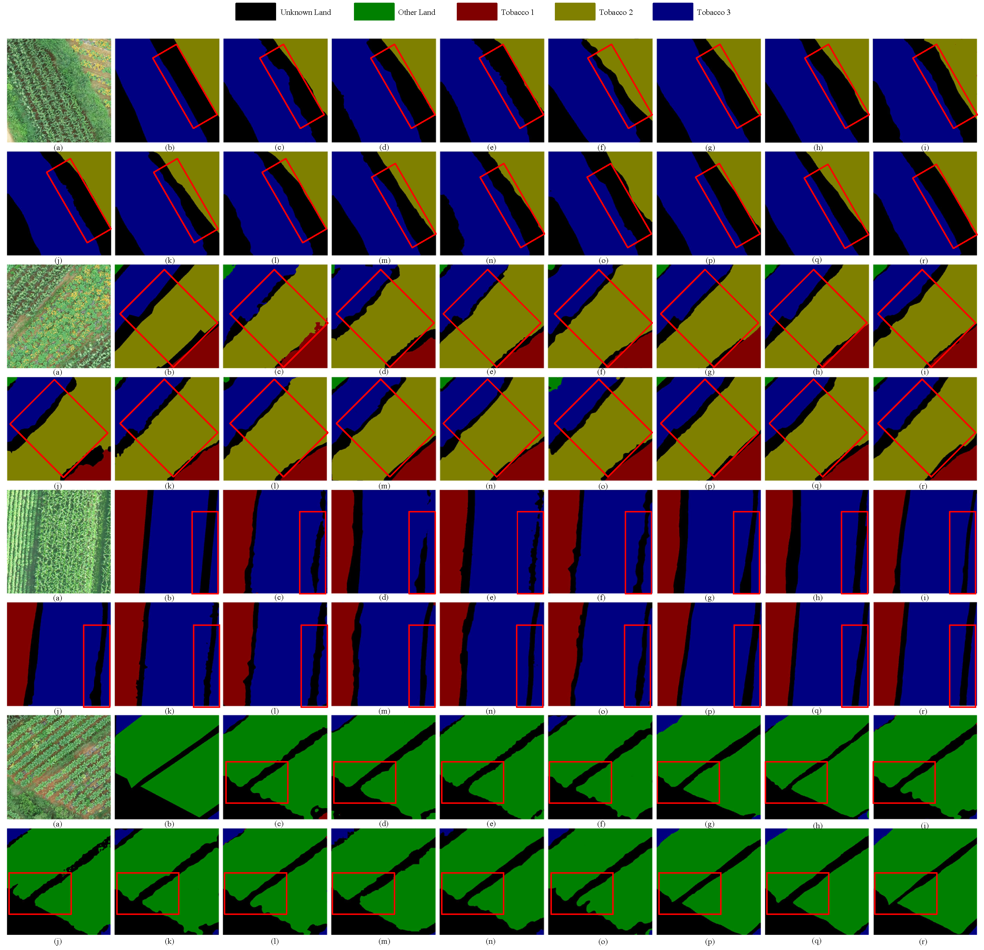
The segmentation results are visualized in Figure 14. In the first and second row, due to the similar color between “Tobacco 2” and the “Background”, “Tobacco 2” is more likely to be misclassified as “Background”. However, by aggregating more discriminative features from frequency domain information and global context, SF3Net perform relatively accurate inference in such challenging cases. In the fifth and sixth row, SF3Net accurately distinguishes “Tobacco 1” and “Tobacco 3” on both sides, outperforming other methods. In the seventh and eighth row, our model demonstrates superior results in recognizing areas with significant texture variation and in segmenting edges, further highlighting its robustness and accuracy in RS image segmentation.

Figure 14. Visualization of segmentation on the Farmland test set: (a) Image, (b) GT, (c) PSPNet, (d) DeepLabV3+, (e) DANet, (f) ABCNet, (g) SegFormer, (h) TransUNet, (i) MAResU-Net, (j) UNetFormer, (k) ST-UNet, (l) PIDNet, (m) CaSaFormer, (n) XNet, (o) SFFNet, (p) RS3Mamba, (q) SegMAN, (r) SF3Net (Ours). There are four sets of results in total in this figure and red boxes indicate key focus areas.

4.2.4. Efficiency Analysis

For a comprehensive comparison, Table 7 lists the parameters of the model and the time of testing on the Vaihingen dataset under the same operating environment. In terms of testing time, SF3Net takes 18.9 s, making it 6.8 s faster than the spatial–frequency fusion network SFFNet with a wavelet decomposer. It is faster than most spatial domain-based segmentation methods, only 1.9 s, 1.5 s and 3.8 s slower than SegFormer, PIDNet and CaSaFormer. Regarding model parameters, as SF3Net adopts a parallel structure for the fusion of spatial and frequency domain features, its parameter count is larger than SegFormer, PIDNet and CaSaFormer but remains smaller than other methods. Its parameters are approximately 4 times fewer than SFFNet, and its FLOPs are about 12 times fewer than SFFNet. Therefore, compared with some segmentation frameworks based solely on spatial domain features, SF3Net does not show significant advantages in terms of model parameters and computational complexity. However, compared with other models that also perform spatial–frequency feature fusion, it reduces both the number of parameters and complexity, achieving a better balance between accuracy and model complexity. In applications where high efficiency is required along with spatial–frequency feature fusion, SF3Net still demonstrates significant effectiveness.

Table 7. Comparison of model parameters and test time.

Method	Parameters (M) ↓	FLOPs (G) ↓	Testing Time(s) ↓
PSPNet	46.604	179.372	19.7
DeepLabV3+	41.219	177.410	31.2
DANet	47.462	211.832	18.4
ABCNet	15.279	56.870	22.3
SegFormer	3.717	7.902	17.0
TransUNet	98.644	229.908	38.4
MAResU-Net	28.346	152.341	24.6
ST-UNet	168.830	492.78	48.3
UNetFormer	11.716	47.026	20.3
PIDNet	7.718	5.933	17.4
CaSaFormer	4.408	1.931	15.1
XNet	78.756	103.780	27.7
SFFNet	34.097	50.696	25.7
RS3Mamba	40.533	37.314	21.4
SegMAN-S	29.404	23.775	20.9
SF3Net	8.454	4.056	18.9
The (↓) represents a degradation in performance.

5. Discussion

Through comprehensive experiments conducted on the Vaihingen, Potsdam, and agricultural datasets, we have thoroughly validated the exceptional capabilities of SF3Net in the field of remote sensing image segmentation. In numerous domains including land resource management, urban planning, and disaster monitoring, efficiency and accuracy remain the core requirements for various tasks. Leveraging the high efficiency and precision characteristics of this method, it demonstrates excellent applicability and outstanding performance in the aforementioned applications, fully showcasing its tremendous potential and promising prospects for widespread application across multiple domains. Furthermore, SF3Net effectively overcomes the limitations inherent in traditional spatial domain segmentation methods by enhancing spatial feature representation and integrating frequency domain features, exhibiting particularly remarkable performance in inferring edge regions and areas with significant texture variations. This advancement further promotes the development in frequency–spatial feature fusion segmentation methods. However, experiments show that while FFSL introduces rich frequency domain information and preserves some local spatial information, the Fourier transform cannot retain fine spatial details when converting the image to the frequency domain, leading to potential missegmentation. Additionally, the Fourier transform requires both frequency domain conversion and inverse conversion, increasing computational overhead and affecting the real-time performance and efficiency of segmentation. On the other hand, the main advantage of SFFM is that it compensates for the spatial information loss caused by FFSL in frequency domain feature learning by fusing SFAM and FFSL. Furthermore, FSM selectively fuses the most relevant shallow features, reducing information loss during the encoder’s downsampling process and further compensating for FFSL’s loss of spatial detail information. In the future, we plan to explore contrastive learning and multimodal techniques to narrow the semantic gap between spatial and frequency domain features, improve fusion efficiency, and ultimately enhance semantic segmentation.

6. Conclusions

In this paper, we propose a novel SF3Net for lightweight spatial–frequency feature fusion in remote sensing semantic segmentation. The network introduces rich frequency-domain features while retaining sufficient spatial features, effectively addressing the challenges of inaccurate segmentation at boundaries and regions with significant grayscale variations by fusing features from two representational domains. Specifically, the proposed FFSL utilizes the fourier transform to extract rich frequency-domain features in three directions. In addition, the SFAM and FSM are designed to further enhance spatial modeling capabilities. SFAM establishes pixel-level information exchange in a weighted manner to alleviate segmentation errors caused by occlusion, while FSM adaptively preserves detailed features that are most relevant to the encoder. Finally, the SFFM fuses frequency-domain features with spatial-domain features, maximizing the combined use of global information and local details. However, the synergistic fusion of frequency-domain and spatial-domain features may, to some extent, limit the efficiency of dual-domain collaborative segmentation. Moreover, the reliance on single-modality remote sensing image data also constrains further improvements in segmentation accuracy. In future work, we plan to explore direct fusion of spatial- and frequency-domain features through semantic alignment, and the incorporation of multimodal remote sensing data to enhance feature fusion efficiency and improve the accuracy of remote sensing image segmentation.

References

1. Zheng, C.; Li, X.; Liang, X.; Huang, L.; Du, S.; Nie, J.; Dong, J. Cross-Modal Progressive Perspective Matching Network for Remote Sensing Image-Text Retrieval. IEEE Trans. Multimed. 2025, 27, 3966–3978. [Google Scholar] [CrossRef]
2. Bi, H.; Xu, F.; Wei, Z.; Xue, Y.; Xu, Z. An active deep learning approach for minimally supervised PolSAR image classification. IEEE Trans. Geosci. Remote Sens. 2019, 57, 9378–9395. [Google Scholar] [CrossRef]
3. Shamsolmoali, P.; Zareapoor, M.; Wang, R.; Zhou, H.; Yang, J. A novel deep structure U-Net for sea-land segmentation in remote sensing images. IEEE J. Sel. Top. Appl. Earth Obs. Remote Sens. 2019, 12, 3219–3232. [Google Scholar] [CrossRef]
4. Hashemi-Beni, L.; Gebrehiwot, A.A. Flood Extent Mapping: An Integrated Method Using Deep Learning and Region Growing Using UAV Optical Data. IEEE J. Sel. Top. Appl. Earth Obs. Remote Sens. 2021, 14, 2127–2135. [Google Scholar] [CrossRef]
5. Huan, H.; Liu, Y.; Xie, Y.; Wang, C.; Xu, D.; Zhang, Y. MAENet: Multiple attention encoder–decoder network for farmland segmentation of remote sensing images. IEEE Geosci. Remote Sens. Lett. 2021, 19, 2503005. [Google Scholar] [CrossRef]
6. Yu, Y.; Bao, Y.; Wang, J.; Chu, H.; Zhao, N.; He, Y.; Liu, Y. Crop Row Segmentation and Detection in Paddy Fields Based on Treble-Classification Otsu and Double-Dimensional Clustering Method. Remote Sens. 2021, 13, 901. [Google Scholar] [CrossRef]
7. Yang, R.; Su, Y.; Zhong, Y. Urban Land-Use Classification with Multi-Source Self-Supervised Representation Learning and Correlation Modeling. In Proceedings of the IGARSS 2024—2024 IEEE International Geoscience and Remote Sensing Symposium, Athens, Greece, 7–12 July 2024; pp. 4693–4696. [Google Scholar]
8. Zhang, P.; Li, J.; Wang, C.; Niu, Y. SAM2MS: An Efficient Framework for HRSI Road Extraction Powered by SAM2. Remote Sens. 2025, 17, 3181. [Google Scholar] [CrossRef]
9. Blaschke, T.; Lang, S.; Hay, G. Object-Based Image Analysis: Spatial Concepts for Knowledge-Driven Remote Sensing Applications; Springer Science & Business Media: Berlin/Heidelberg, Germany, 2008. [Google Scholar]
10. Long, J.; Shelhamer, E.; Darrell, T. Fully convolutional networks for semantic segmentation. In Proceedings of the IEEE Conference on Computer Vision and Pattern Recognition, Boston, MA, USA, 7–12 June 2015; pp. 3431–3440. [Google Scholar]
11. Ronneberger, O.; Fischer, P.; Brox, T. U-net: Convolutional networks for biomedical image segmentation. In Proceedings of the International Conference on Medical Image Computing and Computer-Assisted Intervention, Munich, Germany, 5–9 October 2015; Springer: Berlin/Heidelberg, Germany, 2015; pp. 234–241. [Google Scholar]
12. Huang, Z.; Wang, X.; Huang, L.; Huang, C.; Wei, Y.; Liu, W. Ccnet: Criss-cross attention for semantic segmentation. In Proceedings of the IEEE/CVF International Conference on Computer Vision, Seoul, Republich of Korea, 27 October–2 November 2019; pp. 603–612. [Google Scholar]
13. Fu, J.; Liu, J.; Tian, H.; Li, Y.; Bao, Y.; Fang, Z.; Lu, H. Dual attention network for scene segmentation. In Proceedings of the IEEE/CVF Conference on Computer Vision and Pattern Recognition, Long Beach, CA, USA, 15–20 June 2019; pp. 3146–3154. [Google Scholar]
14. Chen, L.C.; Zhu, Y.; Papandreou, G.; Schroff, F.; Adam, H. Encoder-decoder with atrous separable convolution for semantic image segmentation. In Proceedings of the European Conference on Computer Vision (ECCV), Munich, Germany, 8–14 September 2018; pp. 801–818. [Google Scholar]
15. Nong, Z.; Su, X.; Liu, Y.; Zhan, Z.; Yuan, Q. Boundary-aware dual-stream network for VHR remote sensing images semantic segmentation. IEEE J. Sel. Top. Appl. Earth Obs. Remote Sens. 2021, 14, 5260–5268. [Google Scholar] [CrossRef]
16. Jin, J.; Zhou, W.; Yang, R.; Ye, L.; Yu, L. Edge detection guide network for semantic segmentation of remote-sensing images. IEEE Geosci. Remote Sens. Lett. 2023, 20, 5000505. [Google Scholar] [CrossRef]
17. Mao, Y.Q.; Jiang, Z.; Liu, Y.; Zhang, Y.; Li, Y.; Yan, C.; Zheng, B. Body joint boundary prototype match for few shot remote sensing semantic segmentation. IEEE Geosci. Remote Sens. Lett. 2024, 21, 6016005. [Google Scholar] [CrossRef]
18. Vaswani, A.; Shazeer, N.; Parmar, N.; Uszkoreit, J.; Jones, L.; Gomez, A.N.; Kaiser, L.u.; Polosukhin, I. Attention is All you Need. In Proceedings of the Advances in Neural Information Processing Systems; Guyon, I., Luxburg, U.V., Bengio, S., Wallach, H., Fergus, R., Vishwanathan, S., Garnett, R., Eds.; Curran Associates, Inc.: New York, NY, USA, 2017; Volume 30. [Google Scholar]
19. Wang, W.; Xie, E.; Li, X.; Fan, D.P.; Song, K.; Liang, D.; Lu, T.; Luo, P.; Shao, L. Pyramid Vision Transformer: A Versatile Backbone for Dense Prediction Without Convolutions. In Proceedings of the IEEE/CVF International Conference on Computer Vision (ICCV), Montreal, QC, Canada, 10–17 October 2021; pp. 568–578. [Google Scholar]
20. Cai, H.; Li, J.; Hu, M.; Gan, C.; Han, S. Efficientvit: Lightweight multi-scale attention for high-resolution dense prediction. In Proceedings of the IEEE/CVF International Conference on Computer Vision, Paris, France, 1–6 October 2023; pp. 17302–17313. [Google Scholar]
21. Liu, Z.; Lin, Y.; Cao, Y.; Hu, H.; Wei, Y.; Zhang, Z.; Lin, S.; Guo, B. Swin transformer: Hierarchical vision transformer using shifted windows. In Proceedings of the IEEE/CVF International Conference on Computer Vision, Montreal, BC, Canada, 11–17 October 2021; pp. 10012–10022. [Google Scholar]
22. Lin, R.; Zhang, Y.; Zhu, X.; Chen, X. Local-global feature capture and boundary information refinement swin transformer segmentor for remote sensing images. IEEE Access 2024, 12, 6088–6099. [Google Scholar] [CrossRef]
23. Wang, H.; Chen, X.; Zhang, T.; Xu, Z.; Li, J. CCTNet: Coupled CNN and Transformer Network for Crop Segmentation of Remote Sensing Images. Remote Sens. 2022, 14, 1956. [Google Scholar] [CrossRef]
24. Xu, G.; Li, J.; Gao, G.; Lu, H.; Yang, J.; Yue, D. Lightweight Real-Time Semantic Segmentation Network With Efficient Transformer and CNN. IEEE Trans. Intell. Transp. Syst. 2023, 24, 15897–15906. [Google Scholar] [CrossRef]
25. Hoyer, L.; Dai, D.; Van Gool, L. Daformer: Improving network architectures and training strategies for domain-adaptive semantic segmentation. In Proceedings of the IEEE/CVF Conference on Computer Vision and Pattern Recognition, New Orleans, LA, USA, 18–24 June 2022; pp. 9924–9935. [Google Scholar]
26. Xie, E.; Wang, W.; Yu, Z.; Anandkumar, A.; Alvarez, J.M.; Luo, P. SegFormer: Simple and Efficient Design for Semantic Segmentation with Transformers. In Proceedings of the Advances in Neural Information Processing Systems; Curran Associates, Inc.: New York, NY, USA, 2021; Volume 34, pp. 12077–12090. [Google Scholar]
27. Gu, A.; Dao, T. Mamba: Linear-time sequence modeling with selective state spaces. arXiv 2023, arXiv:2312.00752. [Google Scholar] [CrossRef]
28. Liu, Y.; Tian, Y.; Zhao, Y.; Yu, H.; Xie, L.; Wang, Y.; Ye, Q.; Jiao, J.; Liu, Y. Vmamba: Visual state space model. Adv. Neural Inf. Process. Syst. 2024, 37, 103031–103063. [Google Scholar]
29. Ma, X.; Zhang, X.; Pun, M.O. Rs3 mamba: Visual state space model for remote sensing image semantic segmentation. IEEE Geosci. Remote Sens. Lett. 2024, 21, 6011405. [Google Scholar] [CrossRef]
30. Qin, Z.; Zhang, P.; Wu, F.; Li, X. Fcanet: Frequency channel attention networks. In Proceedings of the IEEE/CVF International Conference on Computer Vision, Montreal, QC, Canada, 10–17 October 2021; pp. 783–792. [Google Scholar]
31. Zhou, Y.; Huang, J.; Wang, C.; Song, L.; Yang, G. XNet: Wavelet-Based Low and High Frequency Fusion Networks for Fully- and Semi-Supervised Semantic Segmentation of Biomedical Images. In Proceedings of the IEEE/CVF International Conference on Computer Vision (ICCV), Paris, France, 1–6 October 2023; pp. 21085–21096. [Google Scholar]
32. Patro, B.N.; Namboodiri, V.P.; Agneeswaran, V.S. Spectformer: Frequency and attention is what you need in a vision transformer. In Proceedings of the 2025 IEEE/CVF Winter Conference on Applications of Computer Vision (WACV), Tucson, AZ, USA, 26 February–6 March 2025; IEEE: Piscataway, NJ, USA, 2025; pp. 9543–9554. [Google Scholar]
33. Yang, Y.; Yuan, G.; Li, J. SFFNet: A Wavelet-Based Spatial and Frequency Domain Fusion Network for Remote Sensing Segmentation. IEEE Trans. Geosci. Remote Sens. 2024, 62, 3000617. [Google Scholar] [CrossRef]
34. Li, X.; Xu, F.; Yu, A.; Lyu, X.; Gao, H.; Zhou, J. A Frequency Decoupling Network for Semantic Segmentation of Remote Sensing Images. IEEE Trans. Geosci. Remote Sens. 2025, 63, 5607921. [Google Scholar] [CrossRef]
35. Sandler, M.; Howard, A.; Zhu, M.; Zhmoginov, A.; Chen, L.C. Mobilenetv2: Inverted residuals and linear bottlenecks. In Proceedings of the IEEE Conference on Computer Vision and Pattern Recognition, Salt Lake City, UT, USA, 18–23 June 2018; pp. 4510–4520. [Google Scholar]
36. Stergiou, A.; Poppe, R.; Kalliatakis, G. Refining activation downsampling with SoftPool. In Proceedings of the IEEE/CVF International Conference on Computer Vision, Montreal, QC, Canada, 10–17 October 2021; pp. 10357–10366. [Google Scholar]
37. Huang, Y.; Zhou, C.; Chen, L.; Chen, J.; Lan, S. Medical frequency domain learning: Consider inter-class and intra-class frequency for medical image segmentation and classification. In Proceedings of the 2021 IEEE International Conference on Bioinformatics and Biomedicine (BIBM), Houston, TX, USA, 9–12 December 2021; IEEE: Piscataway, NJ, USA, 2021; pp. 897–904. [Google Scholar]
38. Rao, Y.; Zhao, W.; Zhu, Z.; Lu, J.; Zhou, J. Global filter networks for image classification. Adv. Neural Inf. Process. Syst. 2021, 34, 980–993. [Google Scholar]
39. Wang, Y.; Liang, B.; Ding, M.; Li, J. Dense Semantic Labeling with Atrous Spatial Pyramid Pooling and Decoder for High-Resolution Remote Sensing Imagery. Remote Sens. 2018, 11, 20. [Google Scholar] [CrossRef]
40. He, X.; Zhou, Y.; Zhao, J.; Zhang, D.; Yao, R.; Xue, Y. Swin transformer embedding UNet for remote sensing image semantic segmentation. IEEE Trans. Geosci. Remote Sens. 2022, 60, 4408715. [Google Scholar] [CrossRef]
41. Fan, L.; Zhou, Y.; Liu, H.; Li, Y.; Cao, D. Combining swin transformer with unet for remote sensing image semantic segmentation. IEEE Trans. Geosci. Remote Sens. 2023, 61, 5530111. [Google Scholar] [CrossRef]
42. Zhao, H.; Shi, J.; Qi, X.; Wang, X.; Jia, J. Pyramid Scene Parsing Network. In Proceedings of the 2017 IEEE Conference on Computer Vision and Pattern Recognition (CVPR), Honolulu, HI, USA, 21–26 July 2017; IEEE: Piscataway, NJ, USA, 2017; pp. 6230–6239. [Google Scholar]
43. Li, R.; Zheng, S.; Zhang, C.; Duan, C.; Wang, L.; Atkinson, P.M. ABCNet: Attentive bilateral contextual network for efficient semantic segmentation of Fine-Resolution remotely sensed imagery. ISPRS J. Photogramm. Remote Sens. 2021, 181, 84–98. [Google Scholar] [CrossRef]
44. Chen, J.; Lu, Y.; Yu, Q.; Luo, X.; Adeli, E.; Wang, Y.; Lu, L.; Yuille, A.L.; Zhou, Y. Transunet: Transformers make strong encoders for medical image segmentation. arXiv 2021, arXiv:2102.04306. [Google Scholar] [CrossRef]
45. Li, R.; Zheng, S.; Duan, C.; Su, J.; Zhang, C. Multistage attention ResU-Net for semantic segmentation of fine-resolution remote sensing images. IEEE Geosci. Remote Sens. Lett. 2021, 19, 8009205. [Google Scholar] [CrossRef]
46. Wang, L.; Li, R.; Zhang, C.; Fang, S.; Duan, C.; Meng, X.; Atkinson, P.M. UNetFormer: A UNet-like transformer for efficient semantic segmentation of remote sensing urban scene imagery. ISPRS J. Photogramm. Remote Sens. 2022, 190, 196–214. [Google Scholar] [CrossRef]
47. Xu, J.; Xiong, Z.; Bhattacharyya, S.P. PIDNet: A real-time semantic segmentation network inspired by PID controllers. In Proceedings of the IEEE/CVF Conference on Computer Vision and Pattern Recognition, Vancouver, BC, Canada, 17–24 June 2023; pp. 19529–19539. [Google Scholar]
48. Li, J.; Hu, Y.; Huang, X. CaSaFormer: A cross-and self-attention based lightweight network for large-scale building semantic segmentation. Int. J. Appl. Earth Obs. Geoinf. 2024, 130, 103942. [Google Scholar] [CrossRef]
49. Fu, Y.; Lou, M.; Yu, Y. SegMAN: Omni-scale context modeling with state space models and local attention for semantic segmentation. In Proceedings of the Computer Vision and Pattern Recognition Conference, Nashville, TN, USA, 10–17 June 2025; pp. 19077–19087. [Google Scholar]
Disclaimer/Publisher’s Note: The statements, opinions and data contained in all publications are solely those of the individual author(s) and contributor(s) and not of MDPI and/or the editor(s). MDPI and/or the editor(s) disclaim responsibility for any injury to people or property resulting from any ideas, methods, instructions or products referred to in the content.
Article Metrics
Citations
Article Access Statistics
Multiple requests from the same IP address are counted as one view.