Article

Semi-BSU: A Boundary-Aware Semi-Supervised Semantic Segmentation Framework with Superpixel Refinement for Coastal Aquaculture Pond Extraction from Remote Sensing Images

1
Aerospace Information Research Institute, Chinese Academy of Sciences (CAS), Beijing 100094, China
2
College of Resources and Environment, University of Chinese Academy of Sciences, Beijing 100049, China
3
Key Laboratory of Earth Observation of Hainan Province, Hainan Aerospace Information Research Institute, Wenchang 571399, China
4
Hainan Aerospace Technology Innovation Center, Wenchang 571333, China
*
Author to whom correspondence should be addressed.
Remote Sens. 2025, 17(22), 3733; https://doi.org/10.3390/rs17223733
Submission received: 15 September 2025 / Revised: 30 October 2025 / Accepted: 12 November 2025 / Published: 17 November 2025

Highlights

What are the main findings?
  • A boundary-aware semi-supervised framework (Semi-BSU) significantly improves the segmentation accuracy of feature edges in remote sensing images, exemplified by coastal aquaculture ponds.
  • Superpixel-guided pseudo-label refinement effectively reduces noise and minimizes intra-class inconsistency.
What is the implication of the main finding?
  • Achieves high-quality remote sensing feature segmentation with minimal labeled samples, exemplified by coastal aquaculture ponds.
  • Provides a practical method for large-scale remote-sensing image interpretation.

Abstract

Accurate segmentation of coastal aquaculture ponds from high-resolution remote sensing images is critical for applications such as coastal environmental monitoring, land use mapping, and infrastructure management. Semi-supervised learning (SSL) has emerged as a promising paradigm by leveraging labeled and unlabeled data to reduce annotation costs. However, existing SSL methods often suffer from pseudo-label quality degradation, manifested as boundary adhesion and intra-class inconsistencies, which significantly affect segmentation accuracy. To address these challenges, we propose Semi-BSU, a boundary-aware semi-supervised semantic segmentation framework based on the mean teacher architecture. Semi-BSU integrates two novel components: (1) a Boundary Consistency Constraint (BCC), which employs an auxiliary boundary classifier to enhance contour accuracy in pseudo labels, and (2) a Superpixel Refinement Module (SRM), which refines pseudo labels at the superpixel level to improve intra-class consistency. Comprehensive experiments conducted on GF6 and ZY1E high-resolution remote sensing imagery, covering diverse coastal environments with complex geomorphological features, demonstrate the effectiveness of our approach. With half of the training set labeled, Semi-BSU achieves an MIOU of 0.8606, F1 score of 0.8896, and Kappa coefficient of 0.8080, outperforming state-of-the-art methods including CPS, GCT, and UniMatch by 0.3–4.9% in MIOU. The method maintains a compact computational footprint with only 1.81 M parameters and 55.71 GFLOPs. Even with only 1/8 labeled data, it yields a 3.57% MIOU improvement over the supervised baseline. The results demonstrate that combining boundary-aware learning with superpixel-based refinement offers an effective and efficient strategy for high-quality pseudo-label generation and accurate mapping of coastal aquaculture ponds in remote sensing imagery.

1. Introduction

Since the 1950s, global aquaculture production has increased substantially, becoming a major source of animal protein and playing an increasingly vital role in the global food security system [1,2]. However, in recent years, the rapid expansion of coastal aquaculture has imposed significant pressure on local coastal ecosystems; among these installations, aquaculture ponds—formed by enclosing tracts of seawater with earthen or concrete embankments—have become a dominant feature. A common development strategy for expanding aquaculture production involves the clearing of mangroves, the alteration of wetlands, and the modification of lakes [3], leading to issues such as habitat destruction [4], loss of biodiversity [5], and water eutrophication [6] in ecosystems like mangroves, wetlands, and lakes. Therefore, it is necessary to conduct scientific monitoring of the location and area of coastal aquaculture ponds.
Remote sensing technology, as an important Earth observation tool [7], plays a crucial role in aquaculture management, primarily applied in three areas: (1) site selection and planning for aquaculture zones based on historical and real-time data; (2) dynamic monitoring of environmental factors in aquaculture zones (such as water quality parameters); and (3) spatial mapping of the distribution of aquaculture facilities of different scales [8,9,10]. These high-precision spatial observation data not only provide scientific basis for research institutions and management departments to understand the development trends of the aquaculture industry but also lay the data foundation for environmental protection policy formulation and resource management decision-making [11]. Spatial distribution information can be obtained through processing of raw remote sensing imagery data, with methods including visual interpretation, spectral classification, object-oriented classification, and deep learning techniques [12]. Visual interpretation relies on visual judgment and comprehensive assessment of remote sensing imagery, requiring the interpreter’s experience and understanding of the color, shape, and texture characteristics of aquaculture areas [13,14]. This method can achieve high-precision results but requires significant human resources and time investment. Spectral classification methods primarily classify the spectral information of each pixel in remote sensing imagery. This method combines remote sensing indices such as NDWI [15,16] and MNDWI [3,17,18] to rapidly identify aquaculture areas in large-scale remote sensing imagery. However, classification results often rely heavily on spectral information, and changes in external lighting or shadows can affect classification accuracy. Additionally, spectral-based methods struggle to capture the overall characteristics of aquaculture ponds, especially when pond shapes are complex and textures vary. Object-oriented classification methods segment aquaculture areas within remote sensing imagery and classify them based on features such as texture and color [19,20,21]. Compared to spectral-based classification methods, this approach better reflects the overall characteristics of aquaculture areas. However, the segmentation algorithms used in this method are highly complex and require significant computational resources; additionally, suitable overall features must be selected subjectively. Deep learning methods automatically perform classification and recognition by learning high-dimensional information about objects in remote sensing images. Among these, some supervised deep learning methods have been extensively applied in the study of coastal aquaculture in recent times [22,23]. Supervised deep learning methods exhibit prominent advantages: they can achieve high segmentation accuracy by leveraging fully labeled data, and their training processes are relatively straightforward with clear optimization objectives, making them reliable baselines for many remote sensing tasks. In the task of identifying coastal aquaculture ponds, some supervised deep learning semantic segmentation networks such as FCN [24], UNet [25,26], and U2-Net [5,27] have achieved good performance.
Supervised semantic segmentation networks perform well in the task of identifying coastal aquaculture ponds, but most methods require large amounts of labeled data for training. Additionally, the models are overly reliant on existing labeled data, leading to insufficient robustness in different scenarios [28]. In recent years, weakly supervised learning methods have been widely applied in remote sensing image scene classification, road extraction, and multi-class object segmentation tasks [29,30,31]. By utilizing low-precision annotation data (such as image-level or sparse point labels) or indirect supervisory signals (such as contextual associations) to train models, these methods significantly reduce the cost and workload associated with high-precision annotations. However, due to the scarcity or ambiguity of supervisory signals, models are prone to learning spurious features, resulting in task accuracy that typically falls below that of fully supervised methods. Compared to supervised and weakly supervised learning, semi-supervised learning not only reduces reliance on fully labeled data but also effectively utilizes a subset of high-precision labeled samples. Semi-supervised learning integrates the features of supervised and unsupervised method, which allows for model training with a substantial quantity of unlabeled data when there is a scarcity of labeled data [32]. If the unlabeled data reaches a certain quantity and the model learns effective information among all data, the accuracy of semi-supervised learning can approach or even exceed that of supervised learning [33]. Semi-supervised learning has made some progress in remote sensing subfields such as building detection [34,35,36] and canopy extraction [37,38,39], but there has been limited research in coastal aquaculture areas. Therefore, exploring the application of semi-supervised learning in identification tasks in coastal aquaculture areas holds significant innovative value and research significance.
Based on existing research, semi-supervised methods primarily include contrastive learning, consistency regularization, and pseudo-labels [40]. Among these, pseudo-label methods typically involve generating pseudo-labels for unlabeled data during training, which are then used to retrain the model. The generation of pseudo-labels generally relies on traditional preprocessing methods, which filter out a large volume of low-confidence information by setting high thresholds. This results in the data features and attributes of the unlabeled data itself not being fully utilized [41,42]. In this paper, the spatial scale of the boundaries of coastal aquaculture ponds is relatively small. If the model lacks sufficient low-level semantic feature extraction capabilities, it may lead to topological errors such as boundary discontinuities or region merging in the pseudo labels. Additionally, isolated high-reflectivity regions may exist within a single aquaculture pond, representing intra-class inconsistency issues. The cause of this issue may be the presence of aeration equipment in aquaculture ponds (Figure 1). During semantic segmentation, the model may misclassify such objects as heterogeneous features, resulting in non-continuous void regions within the aquaculture pond. It is important to note that these aeration devices are inherently part of the aquaculture pond system, and their misclassification directly impacts the integrity and accuracy of the pseudo-labels for the aquaculture pond.
This paper proposes a novel semi-supervised semantic segmentation framework, Semi-BSU, which identifies coastal aquaculture ponds through a self-training mechanism. The core architecture of Semi-BSU is based on the mean teacher model [43]. As a classic framework in the field of semi-supervised learning, Mean-Teacher effectively avoids complex and unstable training processes through its exponential moving average (EMA) mechanism, significantly enhancing training stability compared to other established frameworks like Generative Adversarial Networks (GANs). This characteristic has been extensively validated in semi-supervised segmentation tasks for remote sensing imagery [44,45,46]. This framework achieves predictions on all data through the collaborative training of the teacher and the student model. Specifically, the student model is utilized for training on labeled data and unlabeled data after consistency perturbations, while the teacher model is utilized for training on unlabeled data. During the upsampling stage of the student model, we introduce the boundary consistency constraint (BCC) to ensure that the predicted contours remain spatially consistent. Additionally, we propose the superpixel refinement module (SRM) to optimize the pseudo labels at the superpixel level, addressing the issue of intra-class inconsistency caused by hollow regions within aquaculture ponds.
In summary, this paper proposes a novel semi-supervised learning method, Semi-BSU, to address the following three issues: (1) high annotation costs; (2) pseudo labels prone to boundary breaks or region adhesions; and (3) intra-class inconsistencies in pseudo labels. This paper uses GF6 and ZY1E high-resolution remote sensing imagery as data sources, designing ablation experiments with different components and comparative experiments with advanced semi-supervised learning models to evaluate the contributions of each component module and overall performance. To provide additional validation of the effectiveness of this method, we selected several typical coastal aquaculture zones on Hainan Island, China, to conduct applied research aimed at achieving precise and rapid extraction of aquaculture ponds.

2. Materials and Methods

2.1. Study Area

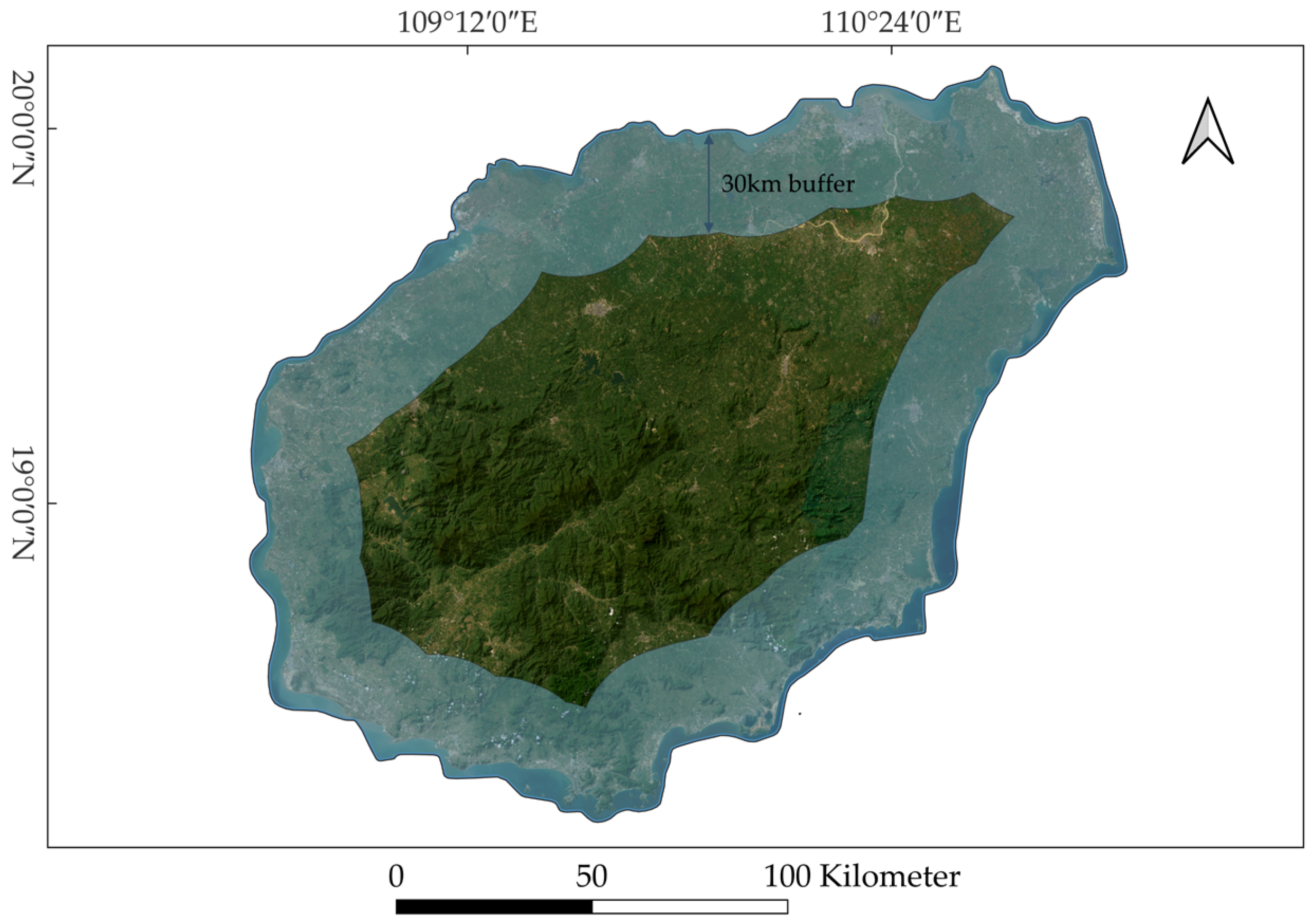
Hainan Island (18°10′–20°10′N, 108°37′–111°03′E) is located at the southernmost tip of China and boasts abundant fishery resources. According to the China Fishery Yearbook 2023, Hainan Province’s fisheries output accounted for 20.5% of its agricultural output in 2022, ranking among the top in the country. Among these, coastal aquaculture output accounted for 17.8%, second only to marine fishing output [47]. Previous studies have shown that a coastal buffer zone of 30 to 50 km can effectively cover coastal aquaculture activities [48,49,50]. Therefore, this study adopts a buffer zone extending 30 km inland from the coastline of Hainan Island as the study area (Figure 2), and selects typical coastal aquaculture scenarios within this zone.

2.2. Dataset and Preprocessing

This paper utilizes high-resolution satellite imagery data to construct a multi-source remote sensing dataset for accurately identifying coastal aquaculture ponds. Specifically, we selected multispectral imagery acquired by the multispectral camera (PMS) of the GF6 satellite and the visible-infrared imaging spectrometer (VIMS) of the ZY1E satellite as the base data, collecting a total of 11 imagery with a time range from 18 January 2024, to 28 September 2024. It is worth noting that although the ZY1E/VIMS sensor provides nine spectral bands, to maintain data consistency with the GF6/PMS sensor (four standard bands), we only extracted and used the four core bands of ZY1E: blue, green, red, and near-infrared. Their technical parameter characteristics are shown in Table 1 below. After undergoing orthorectification and image fusion data preprocessing, we constructed a high-resolution dataset of 1100 images with a size of 224 × 224, including 430 samples from GF6 and 670 samples from ZY1E (Table 2). Typical coastal aquaculture scenarios are mainly divided into estuarine deltas, semi-enclosed seas (such as lagoon types), and coastal bays [51]. To confirm the validity of the method put forward in this study, we selected these typical scenarios mentioned above as experimental areas. As shown in Figure 3, the spatial layout of the samples was determined using a random sampling strategy, covering typical aquaculture areas along the coastal regions of Hainan Island. This ensures that the characteristics of aquaculture ponds in three typical scenarios are adequately represented.

2.3. Methods

2.3.1. Network Architecture

Semi-supervised learning methods can iteratively enhance a model’s unlabeled data understanding and prediction with few labeled samples. In this process, the model first uses the limited labeled data for preliminary training. Subsequently, the trained model is employed to make predictions on unlabeled data and produce pseudo labels. These pseudo labels are then screened and optimized before being reintroduced into the training set to participate in the next round of model training alongside the original labeled data.
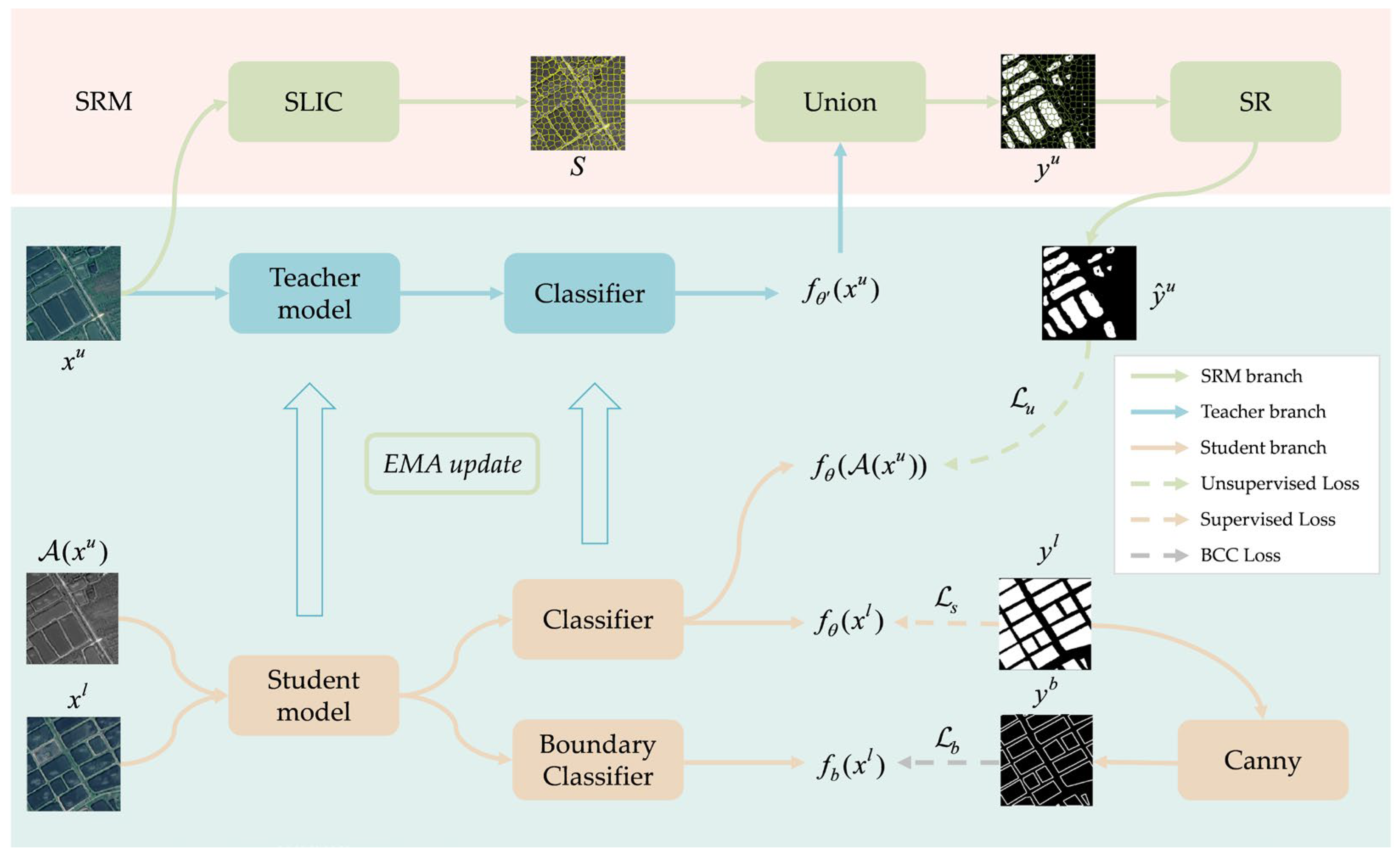
Based on the concept of semi-supervised method, this paper proposes a novel framework, Semi-BSU, which is based on the common mean teacher framework and achieves knowledge transfer and performance optimization through the collaborative training of teacher and student models. Let labeled images be x l C × H × W , labels be y l H × W , and unlabeled images be x u C × H × W (where C is the number of channels, H and W are the height and width of the image, respectively). In each iteration of training, labeled batch data B l = { ( x i l , y i l ) } , unlabeled batch data B u = { x i u } , and consistency-perturbed (Gaussian blur) unlabeled batch data A ( B u ) = { A ( x i u ) } are sampled simultaneously. The teacher model inputs the unlabeled image x u , while the student model inputs two types of data simultaneously: (1) the labeled image x l ; (2) the consistency-perturbed unlabeled image A ( x u ) . The overall architecture is shown in Figure 4. The weights θ of the student model are updated using stochastic gradient descent. Meanwhile, the weights θ of the teacher model can be calculated using exponential moving average (EMA) method as follows:
θ α θ + ( 1 α ) θ
Among these, α is a momentum parameter, which is set to 0.999 based on previous research [43]. In the initial phases of training, the model is just beginning to converge and has weak learning capabilities, which may result in generated pseudo labels containing a significant amount of noise. Therefore, the training process consists of two stages: (1) During the initial training phase, only labeled data is used for pre-training to establish the model’s basic segmentation capabilities. (2) In subsequent stages, both labeled and unlabeled data are utilized for training, enabling the model to fully learn. This EMA update mechanism allows the teacher model to track the learning progress of the student model while maintaining relative stability. The overall loss is calculated as follows:
L = L b + L s + L u
Among these, L b , L s , and L u represent the boundary consistency constraint loss, supervised learning loss, and unsupervised learning loss for labeled data, respectively. The boundary consistency constraint loss is calculated using the boundary prediction f b ( x l ) and boundary map y b from labeled data, while the supervised learning loss is calculated using the standard prediction f θ ( x l ) and true label y l from labeled data. And the unsupervised loss is calculated using the student branch prediction f θ ( A ( x u ) ) and the pseudo label y ^ u of the unlabeled data after consistency perturbations. These will be detailed in Section 2.3.2 and Section 2.3.3.

2.3.2. Student Branch

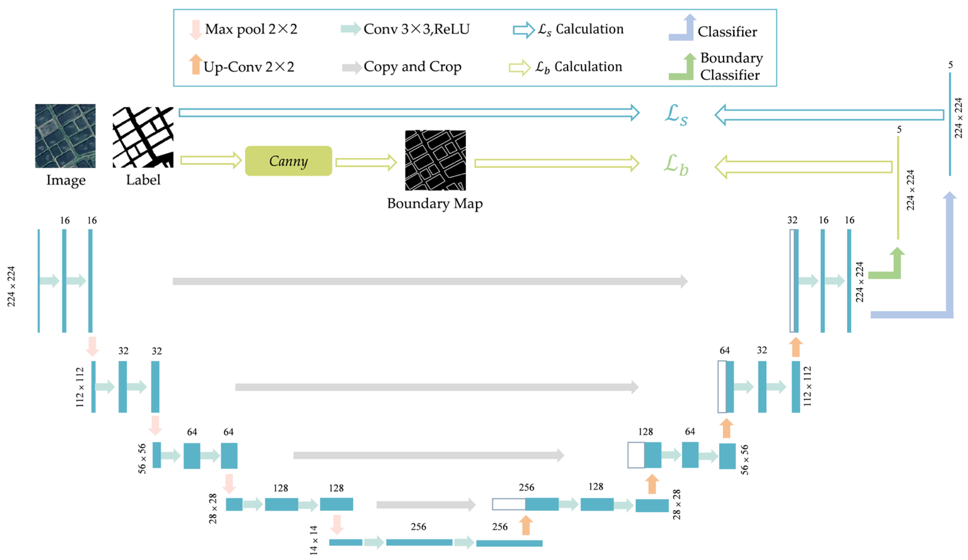
UNet, with its U-shaped convolutional neural network architecture, efficiently accomplishes image segmentation tasks. Originally designed for biomedical image segmentation, the model leverages the similarity between the morphological and distributional characteristics of coastal aquaculture ponds and those of cells in medical images [22]. Consequently, the student branch uses a lightweight UNet as the base model (Figure 5). In the prediction stage of the student branch, a boundary consistency constraint (BCC) is introduced.
Specifically, before the labeled data is input into the student network, the labels are used to generate a true boundary map using the Canny algorithm [52]. The Canny algorithm is a classic and effective method in the field of image boundary detection. Through optimized design, it minimizes boundary false detection rates and achieves precise localization of boundary positions. At its core, the algorithm employs dual-threshold technology for boundary detection and connection. These two thresholds are critical parameters determining its performance, defined as follows: the low threshold filters out non-boundary pixels (pixels below this threshold are deemed non-boundary), while the high threshold identifies strong boundary pixels (pixels above this threshold are classified as strong boundary). Drawing upon relevant research findings on the Canny algorithm in remote sensing image processing [16,53], this study sets the dual thresholds at 0.1 and 0.2, respectively, while retaining all other parameters at their default values.
In addition to the standard prediction output classifier, the model also introduces a boundary classifier to generate a boundary prediction map. The boundary consistency constraint loss is then calculated as follows:
L b = 1 B l i = 1 B l l ( f b ( x i l ) , y i b )
In this context, · represents the set length, l ( · ) denotes the cross-entropy loss function, f b ( x i l ) represents the boundary prediction for the i -th labeled image, and y i b represents the boundary map for the i -th image. Additionally, after the labeled data is input into the student network, it undergoes standard classifier processing to generate probability predictions. In remote sensing images, background pixels often occupy the majority of the image. If only the cross-entropy loss function is used, the model tends to predict all pixels as background. However, Dice Loss can better handle this imbalanced situation, allowing the model to differentiate foreground from background with greater effectiveness [33]. Therefore, the supervised learning loss is calculated as follows:
L s = 1 B l i = 1 B l ( l ( f θ ( x i l ) , y i l ) + D i c e ( s o f t m a x ( f θ ( x i l ) ) , y i l ) )
where f θ ( x i l ) represents the prediction for the i -th labeled image, and y i l represents the corresponding ground truth label for the i -th image.
The unlabeled data enhanced by consistency perturbations is also input into the student branch for training. These data lack corresponding labels, making it impossible to generate true boundary maps. Therefore, when processing this unlabeled data, the model relies solely on the standard classifier for training.

2.3.3. Teacher Branch

The teacher branch adopts the same UNet as the base model for the student branch. However, since the teacher branch processes unlabeled data, the boundary classifier is not employed within the UNet. During the model training phase, unlabeled data is processed through a dual-path collaborative mechanism to optimize pseudo labels: firstly, the teacher branch generates an initial prediction f θ ( x u ) , yielding the original pseudo label:
y u = a r g m a x ( f θ ( x u ) )
At the same time, unlabeled data is input into the SRM branch, processed by the SLIC superpixel segmentation algorithm, and a topological superpixel partition map S = { s i } i = 1 K ( K is the number of superpixels) is generated. Finally, after processing by the superpixel refinement algorithm, more reliable and stable pseudo labels are generated:
y ^ u = S R ( U n i o n ( y u , S ) )
Among them, U n i o n ( · ) is a simple intersection function, and S R ( · ) is a superpixel refinement algorithm, which will be elaborated on in Section 2.3.4. Combining the prediction map generated by the student branch and the pseudo labels generated by the teacher branch, the cross-entropy loss of the unlabeled data is calculated:
L u = λ B u i = 1 B u l ( f θ ( A ( x i u ) ) , y ^ i u )
Among them, f θ ( A ( x i u ) ) represents the i -th prediction graph generated by the student branch, and y ^ i u represents the i -th pseudo label generated by the teacher branch. λ is a weight parameter used to dynamically adjust the contribution of the unsupervised loss. Early in unsupervised training, the model has weak learning ability, leading to a significant amount of noise in the generated pseudo labels [51]. Therefore, a smaller λ is set at the beginning of training and gradually increased as the number of iterations increases. Specifically the Gaussian ramp-up curve [54] is used to calculate:
λ ( t ) = e 5 · ( 1 t T ) 2
Among them, t represents the current training step, T represents total training steps, and λ ( t ) represents the current step’s weight.

2.3.4. Superpixel Refinement

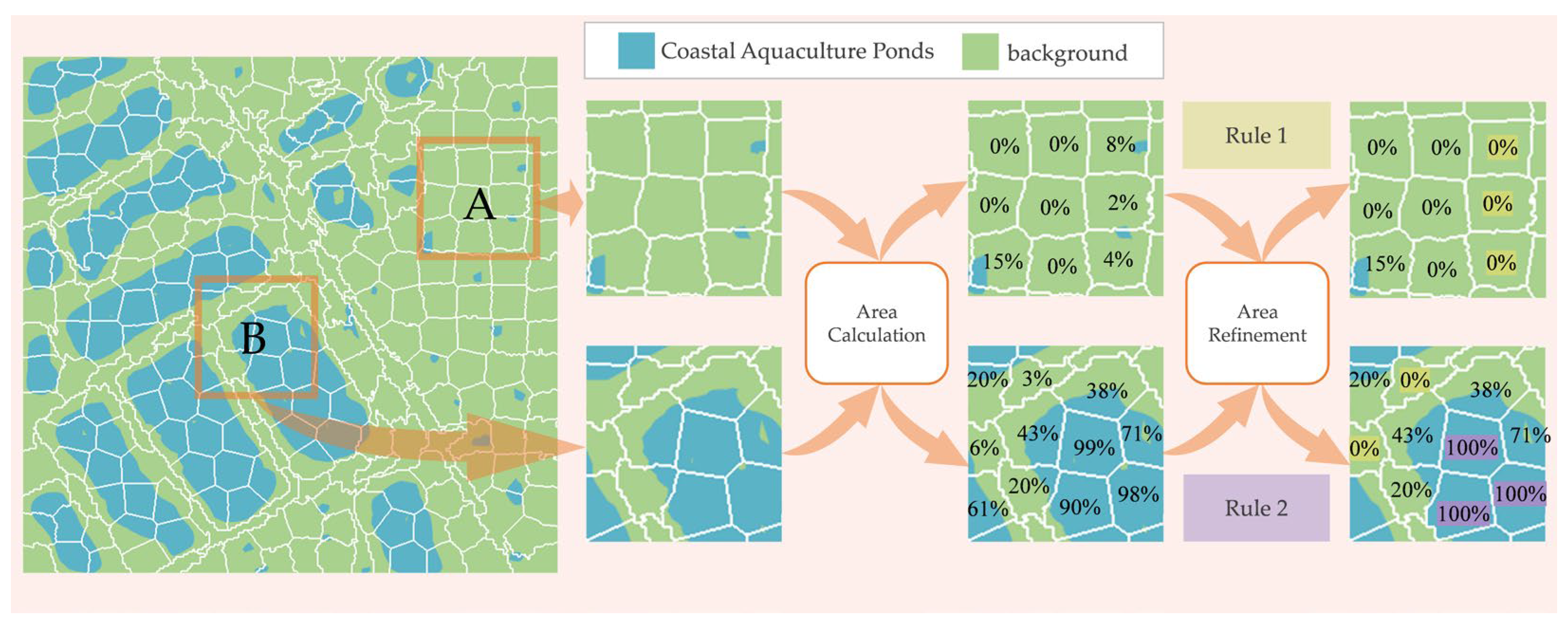
To address the issue of intra-class inconsistency in pseudo labels, this paper proposes a superpixel refinement algorithm. This algorithm divides the initial pseudo labels into multiple superpixel regions and optimizes the area proportions of different classes within each superpixel region. Specifically, it first calculates the area proportions of aquaculture ponds within each superpixel region, Given the pixel set P = { p 1 , p 2 , , p N } (where N is the number of pixels) of the original pseudo label, and the superpixel partition map S = { s 1 , s 2 , , s K } (where K is the number of partitions), for the i -th superpixel partition s i , the area proportion of aquaculture ponds is:
A i = { p j s i | y p j = 1 } s i
Among them, y p j { 0 , 1 } represents the original pseudo label of the j -th pixel (1 for the farming area and 0 for the background). Subsequently, refinement is performed according to rule 1 and 2 (the specific concepts are shown in Figure 6). After refinement, the pseudo label y ^ p j of the j -th pixel is:
y ^ p j = 0 , A i < τ min 1 , A i > τ max p j s i y p j ,   o t h e r w i s e
where τ min represents the lower threshold of the area ratio, and τ max represents the upper threshold of the area ratio, set to 0.1 and 0.9, respectively, the specific rationale for which will be elaborated on in Section 4.2. After refining the pseudo labels of all pixels, a new pseudo label y ^ u is formed:
y ^ u = { y ^ p 1 , y ^ p 2 , , y ^ p N }

3. Results

3.1. Experimental Design

3.1.1. Sample Allocation and Label-Scarcity Simulation

The division of the dataset is a critical step before formally conducting experiments. We randomly divided 1100 images into training, validation, and test sets in an 8:1:1 ratio (Table 3). To systematically evaluate the performance of Semi-BSU, we designed three experiments with progressively increasing labeled data ratios, following previous research [40]: (1) the base group, with a labeled sample ratio of 1/8; (2) the intermediate group, with a labeled sample ratio of 1/4; and (3) the saturated group, with a labeled sample ratio of 1/2.
To reduce overfitting, minimal label-preserving operations (horizontal flip and 90° rotation) are applied only to the labeled images. In the teacher branch, Gaussian blur serves as a consistency perturbation rather than data augmentation, following the standard semi-supervised practice of Mean Teacher.

3.1.2. Implementation Details

In each set of control experiments, we used the same training configuration. The specific parameter settings are as follows: the batch size was uniformly set to 12. The student model was trained using the stochastic gradient descent (SDG) optimizer, with initial learning rate, momentum parameter, and weight decay parameter set to 0.01, 0.9, and 0.0001, respectively. The entire training process consisted of 100 epochs. The model’s learning ability was weak in the initial training stages, leading to generated pseudo labels containing a significant amount of noise. To establish the model’s basic segmentation capabilities, we pre-trained it using only labeled data for the first 10 epochs.

3.1.3. Accuracy Assessment Indicators

We use the quantitative results from the test set as a benchmark to compare the performance of models under different experimental conditions. The evaluation metrics we use include the mean intersection over union ( M I O U ), F 1 score, and K a p p a coefficient. In binary classification tasks, the expressions for these metrics are as follows:
M I O U = 1 2 · ( T N T N + F N + F P + T P T P + F P + F N )
F 1 = 2 T P 2 T P + F P + F N
K a p p a = p o p e 1 p e
Among them, T P is true positive, representing pixels correctly predicted as aquaculture ponds; F P is false positive, representing pixels incorrectly predicted as aquaculture ponds; T N is true negative, representing pixels correctly predicted as background; F N is false negative, representing pixels incorrectly predicted as background. p o is accuracy, p e is expected consistency rate, and their formulas are as follows:
p o = T P + T N T P + T N + F P + F N
P e = ( T P + F N ) ( T P + F P ) + ( F P + T N ) ( F N + T N ) ( T P + T N + F P + F N ) 2

3.2. Experimental Results

3.2.1. Comparison with Different Semi-Supervised Learning Frameworks

As shown in Table 4, we evaluated the performance of various advanced methods under all data ratios using the MIOU, F1, and kappa metrics. All results of these competing methods are derived from our independent reproduction: we followed the network architectures, training schedules, and hyperparameter configurations specified in their original papers to confirm the rationality of our implementation. Overall, as the amount of labeled data increases, the metrics of most methods improve, indicating that larger labeled datasets contribute to enhanced model performance.
The method proposed in this paper, Semi-BSU, demonstrates advantages in multiple aspects. First, at a 1/2 data ratio, its MIOU, F1, and Kappa values are 0.8606, 0.8896, and 0.8080, respectively, all reaching optimal levels. In contrast, the worst-performing UniMatch achieves MIOU, F1, and Kappa of 0.8110, 0.8522, and 0.7340, respectively. Second, even at a 1/4 data ratio, Semi-BSU’s MIOU (0.8554), F1 (0.8876), and Kappa (0.7991) remain leading, while the worst-performing UniMatch achieved MIOU, F1, and Kappa values of 0.7444, 0.8094, and 0.6390, respectively. This indicates that our method maintains high robustness even when labeled data for coastal aquaculture ponds is limited. Additionally, Semi-BSU’s time complexity and space complexity (1.81 M parameters, 55.71 GFLOPs) are significantly lower than other methods, far below GCT (88.98 M parameters, 637.52 GFLOPs) and CPS (80.70 M parameters, 637.52 GFLOPs), indicating its high computational efficiency. This efficiency is particularly important in large-scale coastal aquaculture pond extraction tasks, as such tasks often require massive amounts of remote sensing data and have high real-time requirements. Semi-BSU can achieve real-time, fast, and accurate extraction of coastal aquaculture ponds without consuming excessive computational resources.
However, Semi-BSU performs slightly worse than CPS at an 1/8 data ratio, which may be related to CPS’s cross-pseudo-label supervision mechanism. Under extremely low labeled data conditions, CPS can more effectively control pseudo-label quality through mutual supervision between the two pseudo-label branches [59]. This also indicates that Semi-BSU’s generalization ability under extremely low data conditions still has room for improvement. In the future, more efficient few-shot learning strategies can be explored based on Semi-BSU, or the CPS cross-falsely labeled supervision mechanism can be combined to further optimize the model.
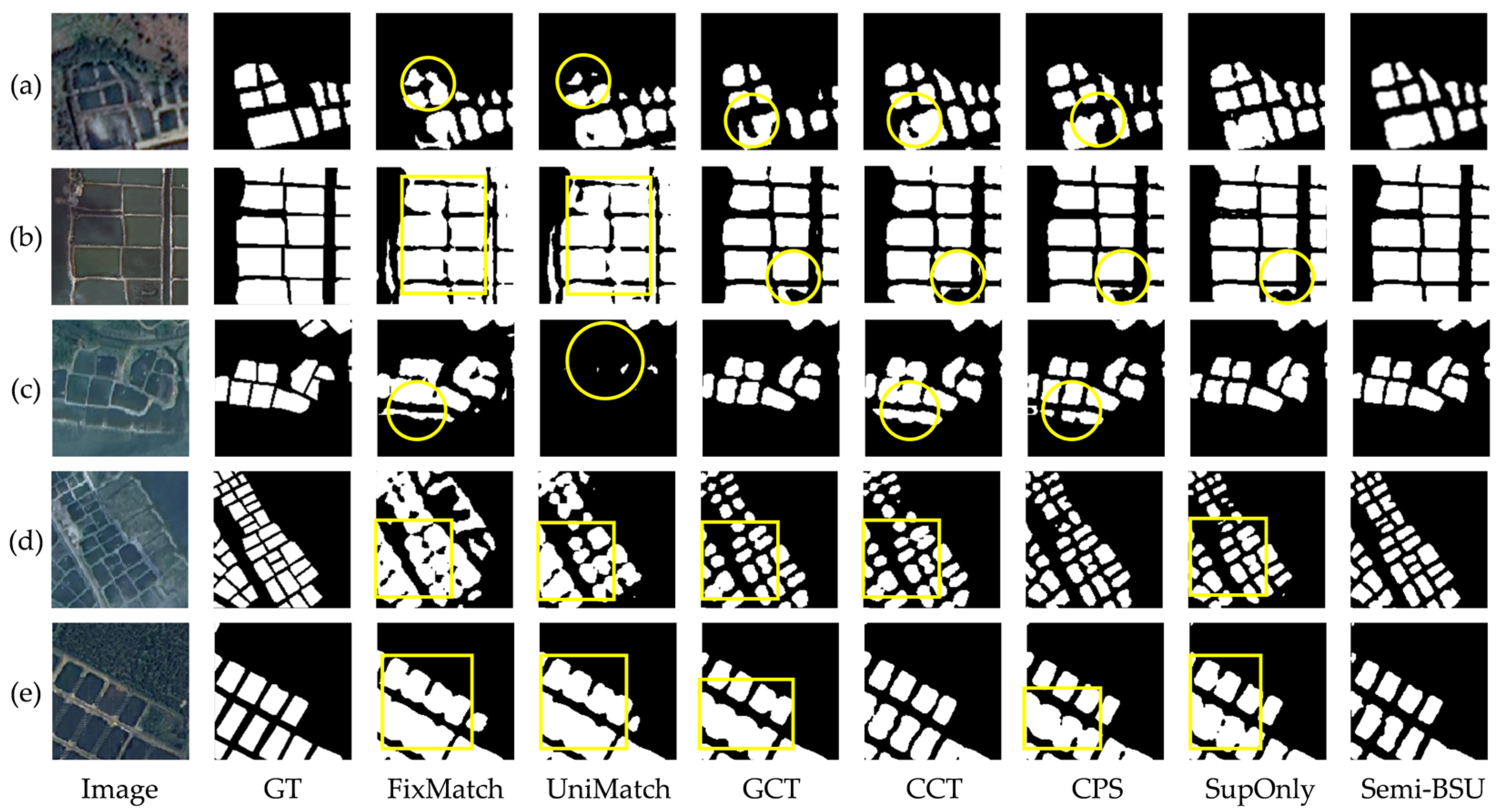
This paper inputs the test set into different trained models and selects multiple scenarios for comparative analysis, as shown in Figure 7. In scenario (a), there is a high-reflectivity region within the circular frame, causing FixMatch, UniMatch, GCT, CCT, and CPS to exhibit varying degrees of fragmented information. However, the Semi-BSU model, which incorporates the SRM, effectively addresses this issue. In scenario (b), due to the narrow boundaries in the central region of the original image, UniMatch and FixMatch produced a significant number of adhesion phenomena in their recognition results. Additionally, there are foreign objects inside the aquaculture pond in the lower right corner of the original image, causing CCT, GCT, CPS, and baseline to identify the pond in that area as fragmented. In scenario (c), FixMatch, CCT, and CPS incorrectly identify the coastal water channel in the original image as an aquaculture pond, while UniMatch exhibits severe missed detection. In scenario (d), the aquaculture ponds in the real image are small in size and densely distributed, leading to varying degrees of boundary adhesion in FixMatch, UniMatch, GCT, CCT, and baseline. Semi-BSU performs notably well, possibly because the BCC effectively captures boundary information. In scenario (e), due to the blurry boundaries of the aquaculture ponds, all models exhibited varying degrees of boundary adhesion. However, overall, Semi-BSU had the least severe boundary adhesion issues. Based on the qualitative analysis results across all scenarios, the Semi-BSU model demonstrated superior performance in the aquaculture pond identification task.

3.2.2. Comparison of Typical Scene Extraction

To further validate the superiority of the Semi-BSU model, this paper takes a 30 km buffer zone extending inland from the coastline of Hainan Island as an example, primarily selecting three typical natural scenarios: coastal bays, estuarine deltas, and semi-enclosed seas, and conducts comparative analyses using different models.
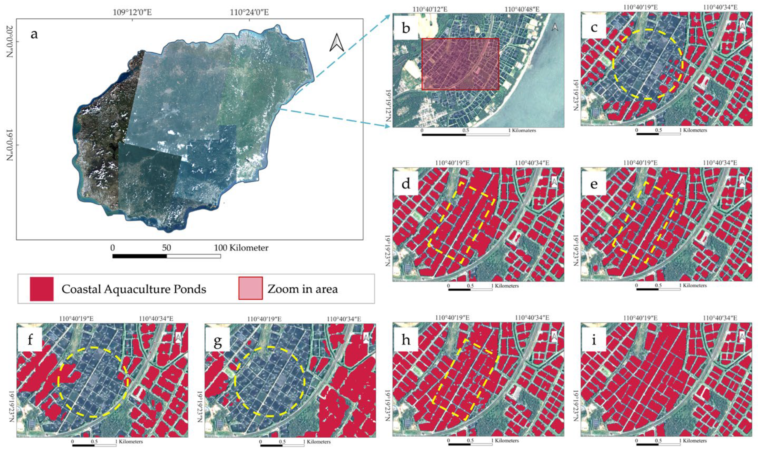
Coastal bays are characterized by extremely dense distributions of aquaculture ponds, with small individual pond areas and narrow, unclear boundaries (Figure 8b). These characteristics impose high demands on the model’s ability to extract low-level semantic features. As shown in Figure 8, within the area marked by the yellow dashed circular, the CCT, FixMatch, and UniMatch models all exhibited severe misclassification phenomena, indicating that these models have limitations in handling fine object recognition in complex backgrounds. Additionally, within the area marked by the yellow dashed rectangular, the GCT, CPS, baseline, and Semi-BSU models all exhibit varying degrees of boundary adhesion issues, which may be attributed to the overly dense distribution of aquaculture ponds in this region. However, the Semi-BSU model, which incorporates BCC, significantly reduces boundary adhesion phenomena, thereby standing out among all models.
Aquaculture ponds in estuarine deltas are primarily distributed in the alluvial island regions of estuaries, where they are relatively sparsely distributed and their boundaries are clearly distinguishable (Figure 9b). As shown in Figure 9, within the area marked by the dashed circular, the FixMatch and UniMatch models exhibit a significant amount of fragmented information, which may be due to their insufficient ability to capture details when processing images with complex textured backgrounds. Meanwhile, the CCT, CPS, and baseline models incorrectly classified the seawater areas near the sand spits as aquaculture ponds, indicating that these models have certain limitations in distinguishing between different water body types. In contrast, the GCT and Semi-BSU models performed the best in this scenario. In particular, the performance advantage of the Semi-BSU model is mainly attributed to its SRM, which can effectively reduce fragmented information during the classification process.
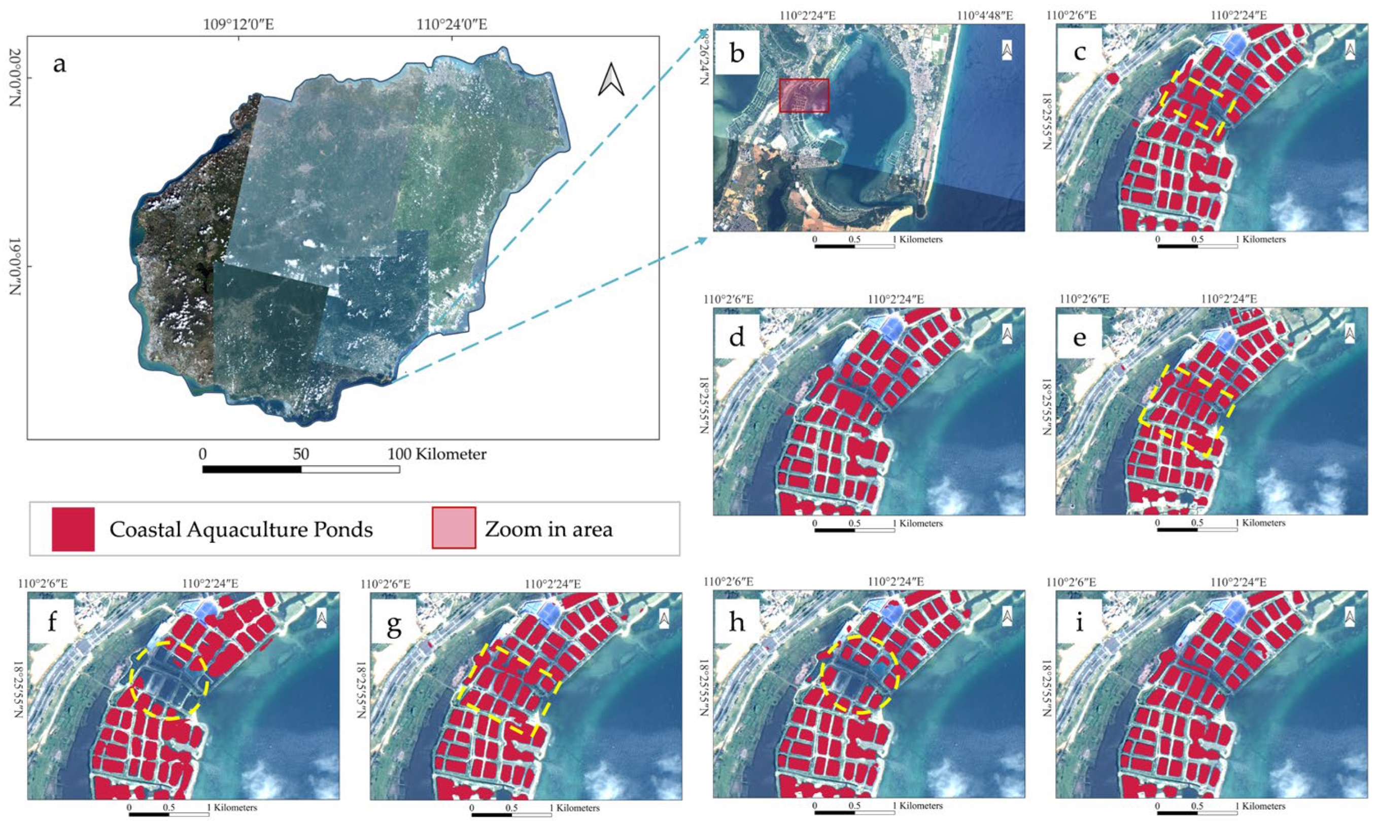
In the semi-enclosed sea (lagoon) scenario, aquaculture ponds are primarily distributed around the edges of the lagoon, and the background information is relatively complex (Figure 10b). As shown in Figure 10, in the circular marked area in the lower left corner, both FixMatch and the baseline model exhibit partial pond detection failures. This is likely attributed to reduced classification accuracy caused by the blurred pond edges in this region. Additionally, CCT, CPS, and UniMatch exhibit boundary coalescence issues in the central rectangular area, likely stemming from unclear boundary features in this zone. In contrast, GCT and Semi-BSU demonstrate fewer errors and superior performance in this scenario. Considering the performance of all models across various scenarios, the Semi-BSU model demonstrated the best overall performance and exhibited higher robustness in the task of identifying aquaculture ponds in complex scenarios.

4. Discussion

4.1. Analysis of Ablation Experiment Results

This paper systematically evaluated the performance of four model configurations by gradually increasing the proportion of labeled data. As shown in Table 5, we gradually introduced BCC and SRM for ablation experiments, using the baseline as a reference. The results are analyzed as follows: (1) The model trained using supervised learning alone serves as the baseline, and the evaluation metrics gradually improve as the proportion of labeled data increases; (2) Adding the BCC (I) improves the evaluation metrics across all labeled data proportions. Notably, a significant improvement is observed at a labeled data proportion of 1/4, with MIOU increasing from 0.8163 to 0.8470, F1 increasing from 0.8455 to 0.8713, and Kappa increasing from 0.7307 to 0.7810. This indicates that boundary information of coastal aquaculture ponds is beneficial for feature learning under moderate data volumes; (3) When the SRM (II) was added, evaluation metrics outperformed the baseline across all data proportions, especially at the 1/8 small data ratio, where MIOU, F1, and Kappa improved by 1.55%, 2.13%, and 3.23%, respectively, demonstrating that the SRM effectively alleviates the issue of insufficient labeled data for aquaculture ponds; (4) The model achieved optimal performance across all data ratios by integrating BCC and the SRM (III). At the 1/2 ratio, MIOU, F1 score, and Kappa reached 0.8606, 0.8896, and 0.8080, respectively, demonstrating the synergistic enhancement effect between modules. Notably, at the 1/8 ratio with the least labeled data, the complete Semi-BSU (III) model achieved a 3.57% improvement in MIOU compared to the baseline, indicating that our proposed method can more effectively utilize limited labeled information. As the data ratio increases, the performance gaps between methods gradually narrow, but the complete model Semi-BSU consistently maintains a leading advantage, demonstrating its robustness across different data scales.
Additionally, we conducted an extra test on the baseline under the Full data ratio, achieving an MIOU of 0.8573. It is worth noting that the complete model Semi-BSU (III) slightly outperformed the baseline under the Full data ratio when tested under the 1/2 data ratio. This phenomenon may be attributed to Semi-BSU’s ability to efficiently extract effective information from unlabeled data in scenarios with scarce labeled data, thereby reducing overfitting to labeled data and maximizing the value of the “small labeled + large unlabeled” data combination. These experimental results fully validate the effectiveness of the BCC and SRM proposed in this paper for the task of identifying coastal aquaculture ponds, particularly in scenarios with complex natural backgrounds or cross-domain learning where labeled data is limited, where they can achieve more significant performance improvements.
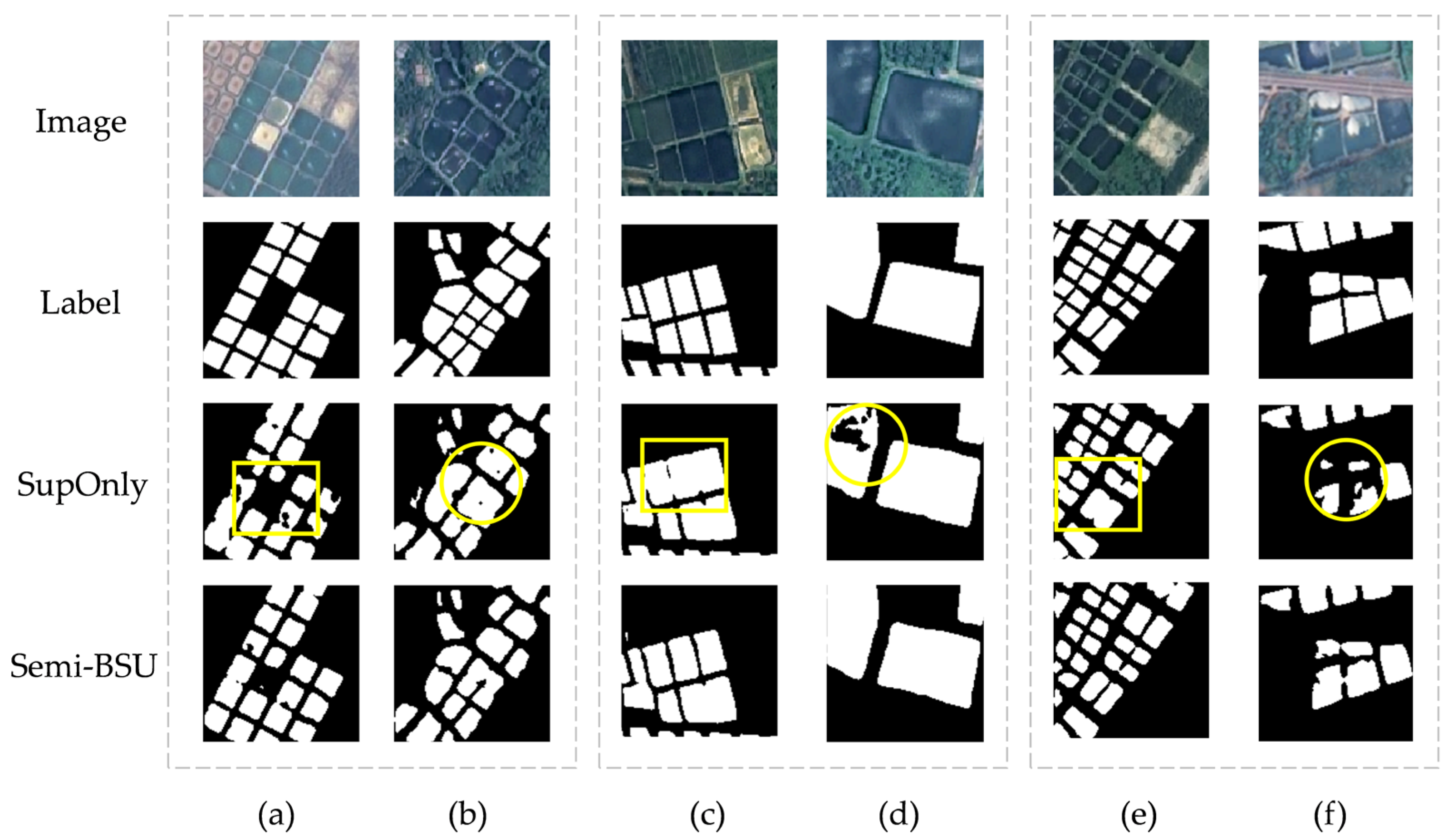
By training on the training set and validation set, we constructed models under various configuration conditions. Subsequently, the test dataset was input into these pre-trained models, and qualitative analyses were conducted under different labeled data ratio conditions, as shown in Figure 11. Scenarios (a,b) illustrate the comparison between the baseline and Semi-BSU model predictions under a 1/8 data ratio, both of which exhibit varying degrees of boundary adhesion and misclassification issues. In particular, the baseline classification results show a more pronounced fragmentation of aquaculture ponds. In contrast, the Semi-BSU model alleviates this issue to some extent. Scenarios (c,d) show the comparison between the baseline and Semi-BSU model predictions at a 1/4 data ratio. The fragmentation phenomenon in the baseline and Semi-BSU model predictions is reduced compared to the 1/8 data ratio, but the baseline still exhibits boundary adhesion and misclassification issues. In the experimental scenario (e,f) with a data ratio of 1/2, the baseline’s prediction results still exhibit the aforementioned issues. In contrast, the Semi-BSU model’s prediction results achieve significant optimization.

4.2. Related Analysis of SRM

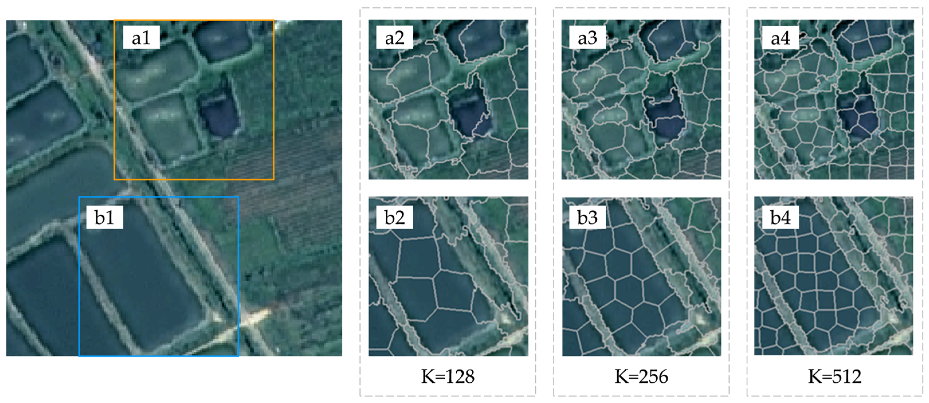
To determine the optimal value of the superpixel count parameter K in the SRM, we designed three sets of comparative experiments with K = 128, K = 256, and K = 512. The results are shown in Figure 12. Analysis of the two typical regions in Figure 12—a1 (smaller pond scene) and b1 (larger pond scene)—reveals the following: (1) When K = 128, the superpixel granularity is too coarse, failing to effectively distinguish ponds from surrounding scenes in both the smaller ponds in a2 and the larger ponds in b2; (2) At K = 512, both a4 and b4 introduced a large number of redundant superpixel blocks, while computational overhead increased; (3) At K = 256, the superpixel segmentation in a3 and b3 preserved relatively complete regional morphology while avoiding superpixel redundancy. Therefore, K = 256 was ultimately selected as the parameter setting for the SRM in this study.
To determine the optimal values for thresholds τ min and τ max in the SRM, this paper references the empirical practice of setting τ max to 0.95 from similar study [60]. Three sets of control experiments were designed around this benchmark: (1) 0.95 and 0.05; (2) 0.90 and 0.10; (3) 0.85 and 0.15, with all other parameters held constant. Using MIOU, F1, and Kappa as evaluation metrics, models incorporating only the SRM were trained. Results are shown in Figure 13. Analysis reveals that the third parameter set performs best under the 1/2 labeled data scenario. This is likely because, with scarce samples, pseudo-label noise increases, and more extreme parameter settings can rigorously filter out erroneous information. However, considering different labeled data ratios, the second parameter set demonstrates overall superior performance: with 1/4 labeled data, its MIOU, F1, and Kappa are significantly higher than the other two sets; and under the 1/2 labeled data scenario, its MIOU and F1 also achieved the best results. Therefore, the second set of parameters is ultimately adopted in this paper, with τ max and τ min set to 0.90 and 0.10, respectively.
Within the semi-supervised learning framework, the quality of pseudo labels plays a crucial role in model performance. To further validate the effectiveness of the SRM, we conducted a visual comparison analysis of pseudo labels before and after optimization during the same training phase. Figure 14a shows a typical image containing local high-reflectivity regions; Figure 14b shows the initial pseudo labels, where the presence of local high-reflectivity regions resulted in a significant number of gaps in the pseudo labels; Figure 14c shows the pseudo labels after superpixel refinement. The comparison demonstrates that the SRM effectively reduces the gaps in pseudo labels caused by local high-reflectivity regions, thereby improving the overall quality of the pseudo labels.

4.3. Related Analysis of BCC

To quantitatively evaluate the contribution of the BCC module to boundary accuracy, this paper introduces the Boundary Intersection over Union (B-IOU) and Boundary F1-score (B-F1) metrics to conduct multiple comparative experiments. B-IOU measures the spatial overlap between predicted and ground-truth boundaries by calculating the ratio of their intersection area to their union area. B-F1 comprehensively evaluates segmentation boundary quality by combining boundary precision and recall. These two metrics provide precise and comprehensive quantification of segmentation boundary quality.
The experimental results are shown in Table 6. Under different labeled sample ratios (1/8, 1/4, 1/2), the method incorporating the BCC module significantly outperformed the SupOnly method in both B-IOU and B-F1 metrics: at the 1/8 ratio, the B-IOU for +BCC was 0.1817 (SupOnly: 0.1739), and B-F1 was 0.2966 (SupOnly: 0.2854). At the 1/4 ratio, B-IOU improved to 0.2198 (SupOnly: 0.1928), and B-F1 increased to 0.3511 (SupOnly: 0.3134). The above results indicate that the introduction of the BCC module effectively improves boundary accuracy.

5. Conclusions

Implementing scientific monitoring of coastal aquaculture ponds is a crucial prerequisite for achieving sustainable management of aquaculture zones. This paper proposes a novel semi-supervised learning framework, Semi-BSU, for identifying coastal aquaculture ponds in high-resolution remote sensing imagery. The framework is based on the mean teacher model and integrates the boundary consistency constraint (BCC) and superpixel refinement module (SRM) to address issues such as pseudo-label boundary adhesion and intra-class inconsistency in semi-supervised learning tasks. Experimental results demonstrate that Semi-BSU performs exceptionally well across various scenarios. Specifically, under most data ratios, Semi-BSU achieves optimal performance when integrated with BCC and SRM modules. At a 1/2 data ratio, Semi-BSU achieves an MIOU of 0.8606, an F1 score of 0.8896, and a Kappa coefficient of 0.8080; at a 1/4 data ratio, its MIOU reaches 0.8554, F1 score reaches 0.8876, and Kappa coefficient reaches 0.7991. Additionally, even under the condition of only 1/8 data proportion, the framework still maintains a certain advantage in performance metrics (MIOU reaches 0.8321, F1 score reaches 0.8587, and Kappa coefficient reaches 0.7558), outperforming other advanced methods (FixMatch, UniMatch, CCT, and GCT). Qualitative analysis further supports these findings, indicating that Semi-BSU effectively reduces boundary adhesion and fragmentation by introducing the BCC and SRM, thereby generating more reliable pseudo labels. Additionally, a visual comparison of prediction results from different models across three distinct typical scenarios—coastal bays, estuarine deltas, and semi-enclosed seas—revealed that Semi-BSU consistently outperforms other models in terms of boundary accuracy and overall classification accuracy for aquaculture ponds. The framework maintains robust performance under complex natural backgrounds and varying data scales, highlighting its practical application value in coastal aquaculture pond extraction tasks.

Author Contributions

Conceptualization, B.C. and Y.G.; methodology, Y.G. and X.Z.; validation, Y.G. and W.F.; formal analysis, B.C. and Y.G.; investigation, Y.G. and W.F.; resources, C.L. and W.F.; data curation, B.C. and X.Z.; writing—original draft preparation, Y.G.; writing—review and editing, B.C., W.F. and C.L.; visualization, Y.G. and W.F.; supervision, B.C. and C.L.; project administration, B.C. and C.L.; funding acquisition, C.L. All authors have read and agreed to the published version of the manuscript.

Funding

Supported by Hainan Province Science and Technology Special Fund (Grant No. ATIC-2023010004).

Data Availability Statement

The data presented in this study are available on request from the corresponding author.

Acknowledgments

The authors would like to thank three anonymous reviewers and the editors for their helpful comments and suggestions, which significantly improved the quality of our paper.

Conflicts of Interest

The authors declare no conflicts of interest.

References

  1. Boyd, C.E.; McNevin, A.A.; Davis, R.P. The contribution of fisheries and aquaculture to the global protein supply. Food Secur. 2022, 14, 805–827. [Google Scholar] [CrossRef]
  2. FAO. Fishery and Aquaculture Statistics Yearbook 2020; FAO: Rome, Italy, 2020. [Google Scholar]
  3. Hou, T.; Sun, W.; Chen, C.; Yang, G.; Meng, X.; Peng, J. Marine floating raft aquaculture extraction of hyperspectral remote sensing images based decision tree algorithm. Int. J. Appl. Earth Obs. Geoinf. 2022, 111, 102846. [Google Scholar] [CrossRef]
  4. Afroz, T.; Alam, S. Sustainable shrimp farming in Bangladesh: A quest for an Integrated Coastal Zone Management. Ocean Coast. Manag. 2013, 71, 275–283. [Google Scholar] [CrossRef]
  5. Zou, Z.; Chen, C.; Liu, Z.; Zhang, Z.; Liang, J.; Chen, H.; Wang, L. Extraction of Aquaculture Ponds along Coastal Region Using U2-Net Deep Learning Model from Remote Sensing Images. Remote Sens. 2022, 14, 4001. [Google Scholar] [CrossRef]
  6. Loisel, H.; Vantrepotte, V.; Ouillon, S.; Ngoc, D.D.; Herrmann, M.; Tran, V.; Mériaux, X.; Dessailly, D.; Jamet, C.; Duhaut, T.; et al. Assessment and analysis of the chlorophyll-a concentration variability over the Vietnamese coastal waters from the MERIS ocean color sensor (2002–2012). Remote Sens. Environ. 2017, 190, 217–232. [Google Scholar] [CrossRef]
  7. Guo, H.; Nativi, S.; Liang, D.; Craglia, M.; Wang, L.; Schade, S.; Corban, C.; He, G.; Pesaresi, M.; Li, J.; et al. Big Earth Data science: An information framework for a sustainable planet. Int. J. Digit. Earth 2020, 13, 743–767. [Google Scholar] [CrossRef]
  8. Kolli, M.K.; Opp, C.; Karthe, D.; Pradhan, B. Automatic extraction of large-scale aquaculture encroachment areas using Canny Edge Otsu algorithm in Google earth engine—The case study of Kolleru Lake, South India. Geocarto Int. 2022, 37, 11173–11189. [Google Scholar] [CrossRef]
  9. Ottinger, M.; Bachofer, F.; Huth, J.; Kuenzer, C. Mapping Aquaculture Ponds for the Coastal Zone of Asia with Sentinel-1 and Sentinel-2 Time Series. Remote Sens. 2021, 14, 153. [Google Scholar] [CrossRef]
  10. Fu, T.; Zhang, L.; Yuan, X.; Chen, B.; Yan, M. Spatio-temporal patterns and sustainable development of coastal aquaculture in Hainan Island, China: 30 Years of evidence from remote sensing. Ocean Coast. Manag. 2021, 214, 105897. [Google Scholar] [CrossRef]
  11. Ottinger, M.; Clauss, K.; Kuenzer, C. Aquaculture: Relevance, distribution, impacts and spatial assessments—A review. Ocean Coast. Manag. 2016, 119, 244–266. [Google Scholar] [CrossRef]
  12. Naylor, R.L.; Hardy, R.W.; Buschmann, A.H.; Bush, S.R.; Cao, L.; Klinger, D.H.; Little, D.C.; Lubchenco, J.; Shumway, S.E.; Troell, M. A 20-year retrospective review of global aquaculture. Nature 2021, 591, 551–563. [Google Scholar] [CrossRef]
  13. Gong, P.; Niu, Z.; Cheng, X.; Zhao, K.; Zhou, D.; Guo, J.; Liang, L.; Wang, X.; Li, D.; Huang, H.; et al. China’s wetland change (1990–2000) determined by remote sensing. Sci. China Earth Sci. 2010, 53, 1036–1042. [Google Scholar] [CrossRef]
  14. Fan, J.; Huang, H.; Fan, H.; Gao, A. Extracting aquaculture area with RADASAT-1. Mar. Sci. 2004, 10, 46–49. [Google Scholar]
  15. Tew, Y.L.; Tan, M.L.; Samat, N.; Chan, N.W.; Mahamud, M.A.; Sabjan, M.A.; Lee, L.K.; See, K.F.; Wee, S.T. Comparison of Three Water Indices for Tropical Aquaculture Ponds Extraction using Google Earth Engine. Sains Malays. 2022, 51, 369–378. [Google Scholar] [CrossRef]
  16. Li, B.; Gong, A.; Chen, Z.; Pan, X.; Li, L.; Li, J.; Bao, W. An Object-Oriented Method for Extracting Single-Object Aquaculture Ponds from 10 m Resolution Sentinel-2 Images on Google Earth Engine. Remote Sens. 2023, 15, 856. [Google Scholar] [CrossRef]
  17. Peng, Y.; Sengupta, D.; Duan, Y.; Chen, C.; Tian, B. Accurate mapping of Chinese coastal aquaculture ponds using biophysical parameters based on Sentinel-2 time series images. Mar. Pollut. Bull. 2022, 181, 113901. [Google Scholar] [CrossRef]
  18. Duan, Y.; Li, X.; Zhang, L.; Chen, D.; Liu, S.a.; Ji, H. Mapping national-scale aquaculture ponds based on the Google Earth Engine in the Chinese coastal zone. Aquaculture 2020, 520, 734666. [Google Scholar] [CrossRef]
  19. Wang, M.; Mao, D.; Xiao, X.; Song, K.; Jia, M.; Ren, C.; Wang, Z. Interannual changes of coastal aquaculture ponds in China at 10-m spatial resolution during 2016–2021. Remote Sens. Environ. 2023, 284, 113347. [Google Scholar] [CrossRef]
  20. Hu, Y.; Zhang, L.; Chen, B.; Zuo, J. An Object-Based Approach to Extract Aquaculture Ponds with 10-Meter Resolution Sentinel-2 Images: A Case Study of Wenchang City in Hainan Province. Remote Sens. 2024, 16, 1217. [Google Scholar] [CrossRef]
  21. Hernandez-Suarez, J.S.; Nejadhashemi, A.P.; Ferriby, H.; Moore, N.; Belton, B.; Haque, M.M. Performance of Sentinel-1 and 2 imagery in detecting aquaculture waterbodies in Bangladesh. Environ. Model. Softw. 2022, 157, 105534. [Google Scholar] [CrossRef]
  22. Yu, J.; He, X.; Yang, P.; Motagh, M.; Xu, J.; Xiong, J. Coastal Aquaculture Extraction Using GF-3 Fully Polarimetric SAR Imagery: A Framework Integrating UNet++ with Marker-Controlled Watershed Segmentation. Remote Sens. 2023, 15, 2246. [Google Scholar] [CrossRef]
  23. Fu, Y.; Ye, Z.; Deng, J.; Zheng, X.; Huang, Y.; Yang, W.; Wang, Y.; Wang, K. Finer Resolution Mapping of Marine Aquaculture Areas Using WorldView-2 Imagery and a Hierarchical Cascade Convolutional Neural Network. Remote Sens. 2019, 11, 1678. [Google Scholar] [CrossRef]
  24. Fu, Y.; You, S.; Zhang, S.; Cao, K.; Zhang, J.; Wang, P.; Bi, X.; Gao, F.; Li, F. Marine aquaculture mapping using GF-1 WFV satellite images and full resolution cascade convolutional neural network. Int. J. Digit. Earth 2022, 15, 2047–2060. [Google Scholar] [CrossRef]
  25. Chen, Y.; Zhang, L.; Chen, B.; Qiu, Y. Information extraction from offshore aquaculture ponds based on improved U-Net model. SmartTech Innov. 2023, 29, 8–14. [Google Scholar] [CrossRef]
  26. Zhang, X.; Dai, P.; Li, W.; Ren, N.; Mao, X. Extracting the images of freshwater aquaculture ponds using improved coordinate attention and U-Net neural network. Trans. Chin. Soc. Agric. Eng. 2023, 39, 153–162. [Google Scholar] [CrossRef]
  27. Chen, C.; Zou, Z.; Sun, W.; Yang, G.; Song, Y.; Liu, Z. Mapping the distribution and dynamics of coastal aquaculture ponds using Landsat time series data based on U2-Net deep learning model. Int. J. Digit. Earth 2024, 17, 2346258. [Google Scholar] [CrossRef]
  28. Liang, C.; Cheng, B.; Xiao, B.; He, C.; Liu, X.; Jia, N.; Chen, J. Semi-/Weakly-Supervised Semantic Segmentation Method and Its Application for Coastal Aquaculture Areas Based on Multi-Source Remote Sensing Images—Taking the Fujian Coastal Area (Mainly Sanduo) as an Example. Remote Sens. 2021, 13, 1083. [Google Scholar] [CrossRef]
  29. Zhou, R.; Zhang, W.; Yuan, Z.; Rong, X.; Liu, W.; Fu, K.; Sun, X. Weakly Supervised Semantic Segmentation in Aerial Imagery via Explicit Pixel-Level Constraints. IEEE Trans. Geosci. Remote Sens. 2022, 60, 5634517. [Google Scholar] [CrossRef]
  30. Lian, R.; Huang, L. Weakly Supervised Road Segmentation in High-Resolution Remote Sensing Images Using Point Annotations. IEEE Trans. Geosci. Remote Sens. 2022, 60, 4501013. [Google Scholar] [CrossRef]
  31. Zhu, Q.; Sun, Y.; Guan, Q.; Wang, L.; Lin, W. A Weakly Pseudo-Supervised Decorrelated Subdomain Adaptation Framework for Cross-Domain Land-Use Classification. IEEE Trans. Geosci. Remote Sens. 2022, 60, 5623913. [Google Scholar] [CrossRef]
  32. Miao, W.; Geng, J.; Jiang, W. Semi-Supervised Remote-Sensing Image Scene Classification Using Representation Consistency Siamese Network. IEEE Trans. Geosci. Remote Sens. 2022, 60, 5616614. [Google Scholar] [CrossRef]
  33. Chen, H.; Li, Z.; Wu, J.; Xiong, W.; Du, C. SemiRoadExNet: A semi-supervised network for road extraction from remote sensing imagery via adversarial learning. ISPRS J. Photogramm. Remote Sens. 2023, 198, 169–183. [Google Scholar] [CrossRef]
  34. Shu, Q.; Pan, J.; Zhang, Z.; Wang, M. MTCNet: Multitask consistency network with single temporal supervision for semi-supervised building change detection. Int. J. Appl. Earth Obs. Geoinf. 2022, 115, 103110. [Google Scholar] [CrossRef]
  35. Sun, C.; Chen, H.; Du, C.; Jing, N. SemiBuildingChange: A Semi-Supervised High-Resolution Remote Sensing Image Building Change Detection Method With a Pseudo Bitemporal Data Generator. IEEE Trans. Geosci. Remote Sens. 2023, 61, 5622319. [Google Scholar] [CrossRef]
  36. Fang, F.; Xu, R.; Li, S.; Hao, Q.; Zheng, K.; Wu, K.; Wan, B. Semisupervised Building Instance Extraction From High-Resolution Remote Sensing Imagery. IEEE Trans. Geosci. Remote Sens. 2023, 61, 5619212. [Google Scholar] [CrossRef]
  37. Guo, J.; Hong, D.; Liu, Z.; Zhu, X.X. Continent-wide urban tree canopy fine-scale mapping and coverage assessment in South America with high-resolution satellite images. ISPRS J. Photogramm. Remote Sens. 2024, 212, 251–273. [Google Scholar] [CrossRef]
  38. Dersch, S.; Schöttl, A.; Krzystek, P.; Heurich, M. Semi-supervised multi-class tree crown delineation using aerial multispectral imagery and lidar data. ISPRS J. Photogramm. Remote Sens. 2024, 216, 154–167. [Google Scholar] [CrossRef]
  39. Amirkolaee, H.A.; Shi, M.; Mulligan, M. TreeFormer: A Semi-Supervised Transformer-Based Framework for Tree Counting From a Single High-Resolution Image. IEEE Trans. Geosci. Remote Sens. 2023, 61, 4406215. [Google Scholar] [CrossRef]
  40. Jiang, S.; Wu, H.; Chen, J.; Zhang, Q.; Qin, J. PH-Net: Semi-Supervised Breast Lesion Segmentation via Patch-Wise Hardness. In Proceedings of the 2024 IEEE/CVF Conference on Computer Vision and Pattern Recognition (CVPR), Seattle, WA, USA, 17–21 June 2024. [Google Scholar]
  41. Luo, F.; Zhou, T.; Liu, J.; Guo, T.; Gong, X.; Gao, X. DCENet: Diff-Feature Contrast Enhancement Network for Semi-Supervised Hyperspectral Change Detection. IEEE Trans. Geosci. Remote Sens. 2024, 62, 5511514. [Google Scholar] [CrossRef]
  42. Wang, Y.; Chen, H.; Heng, Q.; Hou, W.; Fan, Y.; Wu, Z.; Wang, J.; Savvides, M.; Shinozaki, T.; Raj, B.; et al. FreeMatch: Self-Adaptive Thresholding for Semi-Supervised Learning. In Proceedings of the The Eleventh International Conference on Learning Representations (ICLR), Kigali, Rwanda, 1–5 May 2023. [Google Scholar]
  43. Tarvainen, A.; Valpola, H. Mean teachers are better role models: Weight-averaged consistency targets improve semi-supervised deep learning results. In Proceedings of the Advances in Neural Information Processing Systems (NIPS), Long Beach, CA, USA, 4–9 December 2017. [Google Scholar]
  44. Yi, Z.; Wang, Y.; Zhang, L. Revolutionizing Remote Sensing Image Analysis With BESSL-Net: A Boundary-Enhanced Semi-Supervised Learning Network. IEEE Trans. Geosci. Remote Sens. 2023, 61, 5620215. [Google Scholar] [CrossRef]
  45. Zhang, X.; Yang, Y.; Ran, L.; Chen, L.; Wang, K.; Yu, L.; Wang, P.; Zhang, Y. Remote Sensing Image Semantic Change Detection Boosted by Semi-Supervised Contrastive Learning of Semantic Segmentation. IEEE Trans. Geosci. Remote Sens. 2024, 62, 5624113. [Google Scholar] [CrossRef]
  46. Lin, H.; Wang, H.; Yin, J.; Yang, J. Local Climate Zone Classification via Semi-Supervised Multimodal Multiscale Transformer. IEEE Trans. Geosci. Remote Sens. 2024, 62, 5212117. [Google Scholar] [CrossRef]
  47. Affairs, Administration of Fisheries and Fisheries Administration of the Ministry of Agriculture and Rural (Ed.) China Fishery Yearbook; China Agricultural Press: Beijing, China, 2023.
  48. Fu, Y.; Deng, J.; Wang, H.; Comber, A.; Yang, W.; Wu, W.; You, S.; Lin, Y.; Wang, K. A new satellite-derived dataset for marine aquaculture areas in China’s coastal region. Earth Syst. Sci. Data 2021, 13, 1829–1842. [Google Scholar] [CrossRef]
  49. Ren, C.; Wang, Z.; Zhang, Y.; Zhang, B.; Chen, L.; Xi, Y.; Xiao, X.; Doughty, R.B.; Liu, M.; Jia, M.; et al. Rapid expansion of coastal aquaculture ponds in China from Landsat observations during 1984–2016. Int. J. Appl. Earth Obs. Geoinf. 2019, 82, 101902. [Google Scholar] [CrossRef]
  50. Liu, Y.; Wang, Z.; Yang, X.; Zhang, Y.; Yang, F.; Liu, B.; Cai, P. Satellite-based monitoring and statistics for raft and cage aquaculture in China’s offshore waters. Int. J. Appl. Earth Obs. Geoinf. 2020, 91, 102118. [Google Scholar] [CrossRef]
  51. Aguilar-Manjarrez, J.; Soto, D.; Brummett, R. Aquaculture Zoning, Site Selection and Area Management Under the Ecosystem Approach to Aquaculture. A Handbook; FAO: Rome, Italy, 2017. [Google Scholar]
  52. Canny, J.F. A Computational Approach to Edge Detection. IEEE Trans. Pattern Anal. Mach. Intell. 1986, 8, 679–698. [Google Scholar] [CrossRef]
  53. Wang, Z.; Zhang, J.; Yang, X.; Huang, C.; Su, F.; Liu, X.; Liu, Y.; Zhang, Y. Global mapping of the landside clustering of aquaculture ponds from dense time-series 10 m Sentinel-2 images on Google Earth Engine. Int. J. Appl. Earth Obs. Geoinf. 2022, 115, 103100. [Google Scholar] [CrossRef]
  54. Laine, S.; Aila, T. Temporal Ensembling for Semi-Supervised Learning. In Proceedings of the International Conference on Learning Representations (ICLR), Toulon, France, 24–26 April 2017. [Google Scholar]
  55. Sohn, K.; Berthelot, D.; Carlini, N.; Zhang, Z.; Zhang, H.; Raffel, C.A.; Cubuk, E.D.; Kurakin, A.; Li, C.-L. FixMatch: Simplifying Semi-Supervised Learning with Consistency and Confidence. In Proceedings of the Advances in Neural Information Processing Systems (NIPS), Virtual, 6–12 December 2020. [Google Scholar]
  56. Yang, L.; Qi, L.; Feng, L.; Zhang, W.; Shi, Y. Revisiting Weak-to-Strong Consistency in Semi-Supervised Semantic Segmentation. In Proceedings of the 2023 IEEE/CVF Conference on Computer Vision and Pattern Recognition (CVPR), Vancouver, BC, Canada, 18–22 June 2023. [Google Scholar]
  57. Ke, Z.; Qiu, D.; Li, K.; Yan, Q.; Lau, R.W.H. Guided Collaborative Training for Pixel-wise Semi-Supervised Learning. In Proceedings of the European Conference on Computer Vision (ECCV), Glasgow, UK, 23–28 August 2020. [Google Scholar]
  58. Ouali, Y.; Hudelot, C.; Tami, M. Semi-Supervised Semantic Segmentation with Cross-Consistency Training. In Proceedings of the IEEE/CVF Conference on Computer Vision and Pattern Recognition (CVPR), Seattle, WA, USA, 13–19 June 2020. [Google Scholar]
  59. Chen, X.; Yuan, Y.; Zeng, G.; Wang, J. Semi-Supervised Semantic Segmentation with Cross Pseudo Supervision. In Proceedings of the IEEE/CVF Conference on Computer Vision and Pattern Recognition (CVPR), Nashville, TN, USA, 20–25 June 2021. [Google Scholar]
  60. Li, Y.; Yi, Z.; Wang, Y.; Zhang, L. Adaptive Context Transformer for Semisupervised Remote Sensing Image Segmentation. IEEE Trans. Geosci. Remote Sens. 2023, 61, 5621714. [Google Scholar] [CrossRef]
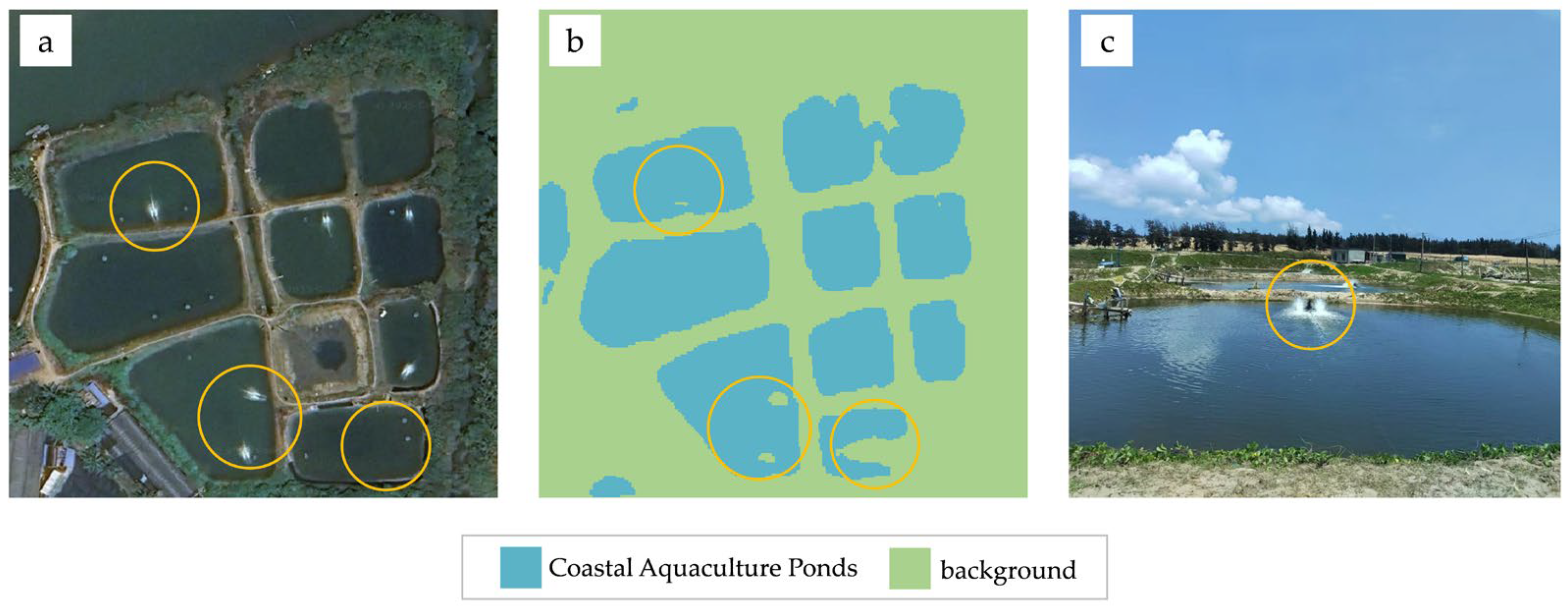
Figure 1. Examples of intra-class inconsistency issues. (a) Remote sensing satellite image; (b) False pseudo labels from traditional semi-supervised models; (c) Field photos. The yellow circular frame indicates high-reflection areas.
Remotesensing 17 03733 g001
Figure 2. Distribution of the 30 km buffer zone extending inland from the coastline of Hainan Island.
Remotesensing 17 03733 g002
Figure 3. Examples of label distributions in three typical scenarios. (ac) Label distributions in three typical natural scenarios—estuarine deltas, semi-enclosed seas, and coastal bays—as observed by the GF6 satellite; (df) Label distributions in three typical scenarios—estuarine deltas, semi-enclosed seas, and coastal bays—as observed by the ZY1E satellite.
Remotesensing 17 03733 g003
Figure 4. Semi-BSU overall framework.
Remotesensing 17 03733 g004
Figure 5. The Unet model with a boundary classifier introduced.
Remotesensing 17 03733 g005
Figure 6. SR algorithm process. Calculate the proportion of aquaculture pond area within each superpixel in each region, and then refine the superpixels using two rules. (A) Shows the application area of rule 1: If the coverage area of aquaculture ponds within a superpixel is less than τ min of the total area, the corresponding aquaculture area will be removed. (B) Shows the application area of rule 2: If the coverage area of aquaculture regions within a superpixel exceeds τ max , all pixels within that superpixel will be classified as aquaculture ponds.
Remotesensing 17 03733 g006
Figure 7. Under the condition of a labeled data ratio of 1/2, a qualitative comparative analysis of the prediction results of various advanced semi-supervised learning models was conducted. The yellow solid circular frame marks the areas where misclassification of aquaculture ponds is particularly severe, while the yellow solid rectangular frame marks the areas where boundary adhesion of aquaculture ponds is particularly severe.
Remotesensing 17 03733 g007
Figure 8. A qualitative comparative analysis of the results obtained from different advanced semi-supervised learning models for extracting aquaculture ponds in coastal bays scenarios under a 1/2 unlabeled data ratio condition. (a) Distribution of coastal bay scenarios; (b) Original imagery; (c) CCT; (d) GCT; (e) CPS; (f) FixMatch; (g) UniMatch; (h) SupOnly; (i) Semi-BSU. Yellow dashed circle indicates areas with severe misclassification of aquaculture ponds, while yellow dashed rectangles indicate areas with severe boundary adhesion of aquaculture ponds.
Remotesensing 17 03733 g008
Figure 9. A qualitative comparative analysis of the results obtained from different advanced semi-supervised learning models for extracting aquaculture ponds in estuarine deltas scenarios under a 1/2 unlabeled data ratio condition. (a) Distribution of estuarine delta scenarios; (b) Original imagery; (c) CCT; (d) GCT; (e) CPS; (f) FixMatch; (g) UniMatch; (h) SupOnly; (i) Semi-BSU. Yellow dashed circle indicates areas with severe misclassification of aquaculture ponds.
Remotesensing 17 03733 g009
Figure 10. A qualitative comparative analysis of the results obtained from different advanced semi-supervised learning models for extracting aquaculture ponds in semi-enclosed sea scenarios under a 1/2 unlabeled data ratio condition. (a) Distribution of semi-enclosed sea scenarios; (b) Original imagery; (c) CCT; (d) GCT; (e) CPS; (f) FixMatch; (g) UniMatch; (h) SupOnly; (i) Semi-BSU. Yellow dashed circle indicates areas with severe misclassification of aquaculture ponds, while yellow dashed rectangles indicate areas with severe boundary adhesion of aquaculture ponds.
Remotesensing 17 03733 g010
Figure 11. Under different proportions of labeled data conditions, qualitative comparative analysis of the prediction results of the baseline and Semi-BSU models is conducted. (a,b) 1/8 data ratio; (c,d) 1/4 data ratio; (e,f) 1/2 data ratio. The yellow solid circular boxes indicate regions where misclassification of aquaculture ponds is more severe, and the yellow solid rectangular boxes indicate areas where the boundary adhesion of aquaculture ponds is more severe.
Remotesensing 17 03733 g011
Figure 12. Comparison of segmentation results for aquaculture pond scenes under different superpixel count settings K. (a1) Original region 1 with small aquaculture ponds (marked by orange frame); (a2) Segmentation result of region 1 with K = 128; (a3) Segmentation result of region 1 with K = 256; (a4) Segmentation result of region 1 with K = 512; (b1) Original region 2 with large aquaculture ponds (marked by blue frame); (b2) Segmentation result of region 2 with K = 128; (b3) Segmentation result of region 2 with K = 256; (b4) Segmentation result of region 2 with K = 512.
Remotesensing 17 03733 g012
Figure 13. Performance comparison of the SRM under different threshold combinations—τ(0.85, 0.15), τ(0.90, 0.10), and τ(0.95, 0.05)—across three labeled ratio scenarios: (a) MIOU metric; (b) F1 metric; (c) Kappa metric.
Remotesensing 17 03733 g013
Figure 14. Under a 1/2 labeled data ratio, a qualitative analysis comparison was conducted on the pseudo labels generated before and after using the SRM. (a) Original image; (b) Original pseudo-label; (c) Refined pseudo-label. The yellow solid line circle indicates areas where misclassification of aquaculture ponds is particularly severe.
Remotesensing 17 03733 g014
Table 1. Technical parameters and features of GF6 and ZY1E.
SatelliteGF6ZY1E
ResolutionSpectral RangeResolutionSpectral Range
Pan2 m450–900 nm2.5 m452–902 nm
SpectralBlue8 m450–520 nm10 m452–521 nm
Green8 m520–600 nm10 m522–607 nm
Red8 m630–690 nm10 m635–694 nm
NIR8 m760–900 nm10 m766–895 nm
Table 2. Parameter characteristics of the sample dataset.
SatelliteSizeResolutionNumber
GF6224 × 2242 m430
ZY1E224 × 2242.5 m670
Table 3. Sample distribution of training, validation, and test sets under different data ratios.
Labeled RatioTrain SetValidation SetTest Set
LabeledUnlabeled
Full880——110110
1/2440440110110
1/4220660110110
1/8110770110110
Table 4. Under different labeled data ratios, we conducted a quantitative comparative analysis of multiple advanced semi-supervised learning models.
Method1/81/41/2ParamsFLOPs
MIOUF1KappaMIOUF1KappaMIOUF1Kappa
FixMatch [55]0.75640.81490.65580.75140.81390.65310.80930.85790.738240.35 M478.14 G
UniMatch [56]0.75760.80660.64800.74440.80940.63900.81100.85220.734040.35 M637.52 G
GCT [57]0.80900.83280.70680.85130.87370.78540.85040.87320.784088.98 M637.52 G
CCT [58]0.79480.83500.70440.83140.85940.75750.84230.86660.771640.35 M159.38 G
CPS [59]0.83460.86230.76390.85420.87710.79240.85760.88780.804080.70 M637.52 G
Semi-BSU0.83210.85870.75580.85540.88760.79910.86060.88960.80801.81 M55.71 G
Bolded values in the table indicate the optimal results for the corresponding metrics.
Table 5. Ablation study using different components under different labeled data.
MethodBCCSRM1/81/41/2Full
MIOUF1KappaMIOUF1KappaMIOUF1KappaMIOUF1Kappa
SupOnly 0.79640.82700.69470.81630.84550.73070.83660.86200.76200.85730.88700.8027
I 0.79690.83510.70170.84700.87130.78100.84070.86560.7696——————
II 0.81190.84830.72700.84760.87810.79400.85070.88090.7911——————
III0.83210.85870.75580.85540.88760.79910.86060.88960.8080——————
Bolded values in the table indicate the optimal results for the corresponding metrics.
Table 6. Ablation study of BCC Module under different labeled data.
Method1/81/41/2Full
B-IOUB-F1B-IOUB-F1B-IOUB-F1B-IOUB-F1
SupOnly0.17390.28540.19280.31340.20130.32580.23600.3726
+BCC0.18170.29660.21980.35110.20750.3346————
Bolded values in the table indicate the optimal results for the corresponding metrics.
Disclaimer/Publisher’s Note: The statements, opinions and data contained in all publications are solely those of the individual author(s) and contributor(s) and not of MDPI and/or the editor(s). MDPI and/or the editor(s) disclaim responsibility for any injury to people or property resulting from any ideas, methods, instructions or products referred to in the content.