Article

OptiFusionStack: A Physio-Spatial Stacking Framework for Shallow Water Bathymetry Integrating QAA-Derived Priors and Neighborhood Context

1
College of Marine Science and Ecological Environment, Shanghai Ocean University, Shanghai 201306, China
2
Shanghai Engineering Research Center of Estuarine and Oceanographic Mapping, Shanghai 201306, China
3
School of Geographical Sciences, China West Normal University, Nanchong 637009, China
4
Sichuan Provincial Engineering Laboratory of Monitoring and Control for Soil Erosion in Dry Valleys, China West Normal University, Nanchong 637009, China
5
School of Geospatial Information, Information Engineering University, No. 62, Kexue Road, Zhengzhou 450001, China
6
School of Information Science and Technology, Hainan Normal University, Haikou 571158, China
*
Author to whom correspondence should be addressed.
Remote Sens. 2025, 17(22), 3712; https://doi.org/10.3390/rs17223712
Submission received: 29 September 2025 / Revised: 1 November 2025 / Accepted: 10 November 2025 / Published: 14 November 2025

Highlights

What are the main findings?
  • OptiFusionStack fuses QAA-derived IOPs with multi-scale neighborhood features and ensemble learning, overcoming the limits of pixel-wise SDB.
  • The framework achieves substantially higher accuracy and spatially coherent maps (e.g., R2 up to 0.9167), validated across optically diverse sites.
What are the implications of the main findings?
  • Incorporating spatial context is as critical as physical priors for reliable and interpretable SDB.
  • The approach shows strong potential for operational coastal mapping in regions with limited or no in situ calibration data.

Abstract

Conventional pixel-wise satellite-derived bathymetry (SDB) models face dual challenges: physical ambiguity from variable water quality and spatial incoherence from ignoring geographic context. This study addresses these limitations by proposing and validating OptiFusionStack, a novel two-stage physio-spatial synergistic framework that operates without in situ optical data for model calibration. The framework first generates diverse, physics-informed predictions by integrating Quasi-Analytical Algorithm (QAA)-derived inherent optical properties (IOPs) with multiple base learners. Critically, it then constructs a multi-scale spatial context by computing neighborhood statistics over an experimentally optimized 9 × 9-pixel window. These physical priors and spatial features are then effectively fused by a StackingMLP meta-learner. Validation in optically diverse environments demonstrates that OptiFusionStack significantly surpasses the performance plateau of pixel-wise methods, elevating inversion accuracy (e.g., R2 elevated from 0.66 to >0.92 in optically complex inland waters). More importantly, the framework substantially reduces spatial artifacts, producing bathymetric maps with superior spatial coherence. A rigorous benchmark against several state-of-the-art, end-to-end deep learning models further confirms the superior performance of our proposed hierarchical fusion architecture in terms of accuracy. This research offers a robust and generalizable new approach for high-fidelity geospatial modeling, particularly under the common real-world constraint of having no in situ data for optical model calibration.

1. Introduction

Shallow-water bathymetry (SDB) is crucial for coastal navigation, marine engineering, benthic habitat monitoring, and climate adaptation [1,2,3]. Traditional shipborne surveys are accurate but costly and spatially limited. Multispectral satellites (e.g., Landsat, Sentinel-2) enable large-scale, repeatable SDB mapping, and have become the primary tool for operational applications and research [4,5,6]. A recent review noted the rapid development of SDB driven by advanced sensors and improved methods, and SDB now applies to more marine environments [7,8,9]. For instance, Pacheco et al. [10] used Landsat 8 for nearshore bathymetry retrieval, while Xu et al. [11,12] mapped extensive areas without in-situ data, addressing data scarcity in remote regions [13,14].
Optical SDB leverages wavelength-dependent light attenuation in water, and satellite spectral signals contain depth-related information [15,16,17]. Early methods such as the Lyzenga model perform well in clear waters but lose accuracy in optically complex areas [18,19,20]. Phytoplankton, suspended sediments, and colored dissolved organic matter (CDOM) distort depth-related signals [21,22]. Two technical approaches have been proposed to enhance robustness.
Physics-informed semi-analytical algorithms (SAAs) retrieve inherent optical properties (IOPs) as physical priors, which separate the effects of water quality and depth [23,24,25]. The Quasi-Analytical Algorithm (QAA) is a core method: Lee et al. [24] first retrieved IOPs from water color in deep waters using QAA, and subsequent studies optimized QAA for shallow water applications [26,27]. For example, Wang et al. [28] improved bathymetric inversion for Weizhou Island using ZY-3 and WorldView-3 data, Zhang et al. [25] integrated high-resolution data with QAA-derived IOPs, and Wu et al. [29] updated QAA and integrated it with machine learning [30]. However, uncalibrated QAA-derived IOPs exhibit biases in the absence of local in-situ data, and these biases impair bathymetric inversion results [16,31]. Qiu et al. [30] noted challenges in retrieving parameters such as diffuse attenuation coefficients in complex coastal waters.
Data-driven machine learning models (e.g., Random Forest, XGBoost) learn nonlinear spectral-depth relationships and adapt well to complex optical conditions [32,33,34]. Recent studies have advanced this field: Kwon et al. [35] used Sentinel-2 data and the Random Forest algorithm for bathymetry in South Korean coastal areas, Eugenio et al. [36] demonstrated that ensemble methods are more effective, and Liang et al. [37] proposed an improved model for turbid waters [38]. Deep learning has also been applied in this field: Zhu et al. [34] reviewed its application in remote sensing, and Cheng et al. [39] employed a stacking ensemble method for SDB in coral reef areas [21].
Two key research gaps persist. First, uncertain physical priors: Uncalibrated QAA-derived IOPs exhibit biases that impair bathymetric inversion [19,25,40]. Shen et al. [41] noted that physics-based models still struggle with variable water quality. Second, neglected spatial autocorrelation: Most methods adopt pixel-wise assumptions and fail to account for the continuity of the seabed and optical fields, leading to spatially incoherent maps (e.g., noise, data gaps) in complex areas [5,21,41]. Hedley [4] noted that such incoherence limits the application of SDB, while Hsu et al. [21] highlighted challenges related to multi-source data fusion [42,43]. Zhao et al. [42] and Wang et al. [44] attempted to address data scarcity but lacked integration of physical and spatial information [22,38].
To address these two issues, this study proposes OptiFusionStack, a novel two-stage physio-spatial synergistic framework. Stage 1: Combine QAA_v6-derived IOPs (e.g., K d , a d g ( 490 ) , a p h y ( 490 ) ) with Sentinel-2 spectral bands and train diverse base learners (Random Forest, XGBoost, SVR, CatBoost). Stage 2: Construct multi-scale spatial context using statistics (mean, standard deviation, minimum, maximum) from a 9 × 9 window—this window balances context capture and noise suppression—then use a StackingMLP meta-learner to fuse features and base model outputs, generating coherent bathymetric maps [44,45].

2. Materials and Methods

2.1. Study Areas and Datasets

The three study areas were strategically selected to rigorously evaluate the OptiFusionStack framework’s performance, robustness, and generalizability across distinctly different and challenging optical environments (Figure 1). A core selection criterion was the availability of high-density, high-accuracy in situ bathymetric data to serve as ground truth. High-quality datasets of this nature, particularly those from multibeam echosounder surveys, are typically collected over well-defined, limited areas for specific engineering or research objectives. Consequently, the geographical extents of the study areas were intentionally delineated to ensure precise spatial co-registration between the ground-truth soundings and the corresponding satellite imagery. Collectively, these sites provide a comprehensive testbed, spanning from a moderately turbid coastal harbor and an optically complex inland river to clear offshore waters.

2.1.1. Nanshan Port (Coastal Harbor)

Nanshan Port, located at 18°19′15.375″N, 109°07′50.340″E in Sanya City, Hainan Province, China, is the closest deep-water port to the 1000-m isobath of the South China Sea. The study area is characterized by moderately turbid water and a depth range of 0–13 m, making it suitable for shallow-water bathymetry research. The seabed consists primarily of fine-grained sediment, and the terrain is gently sloping with no drastic undulations.
In situ bathymetric data were acquired from 11–13 July 2022, using a R2Sonic 2024 multibeam echosounder equipped with an Octans motion compensation system, providing a vertical resolution of 0.15 m. The corresponding satellite remote sensing data consist of a Sentinel-2B image acquired on 4 September 2022 (T49QBA).

2.1.2. Yellow River–Yiluo River Confluence (Optically Complex Inland River)

The second study area is located at the confluence of the Yellow River mainstream and the Yiluo River in Heluo Town, Gongyi City, Henan Province, China (34°48′18.6″N, 112°51′54.3″E). In this region, the interaction between clear water from the Yiluo River and highly sediment-laden water from the Yellow River creates a complex underwater topography from sediment deposition. The water depth ranges from 0 to 9 m, making this site ideal for validating bathymetric methods in optically complex inland waters. The satellite imagery for this study was acquired in October, a period corresponding to relatively low water and sediment discharge for the Yellow River compared to the flood season. Despite this seasonal variation, the water’s optical properties remain highly complex due to multiple contributing factors.
In situ bathymetric data were acquired across 12 cross-sections on 15 June 2024, using a 600 kHz RDI Acoustic Doppler Current Profiler (ADCP) with a vertical resolution of 0.1 m. The corresponding satellite data are a Sentinel-2B image acquired on 23 October 2024 (T49SFU).

2.1.3. Qilian Islands (Clear Offshore Water)

The third study area comprises the Qilian Islands, an offshore reef group in the northern South China Sea. This area is characterized by high water transparency and excellent water quality. The seabed consists predominantly of coral reefs, with a wide depth range (0–40 m) and gentle underwater terrain.
In situ bathymetric data were acquired on 20 July 2019, using a HY1600 single-beam echosounder with a detection accuracy of 0.12 m. The corresponding Sentinel-2B image was acquired on 27 October 2019 (T49QFU).

2.2. Overall Design of the OptiFusionStack Framework

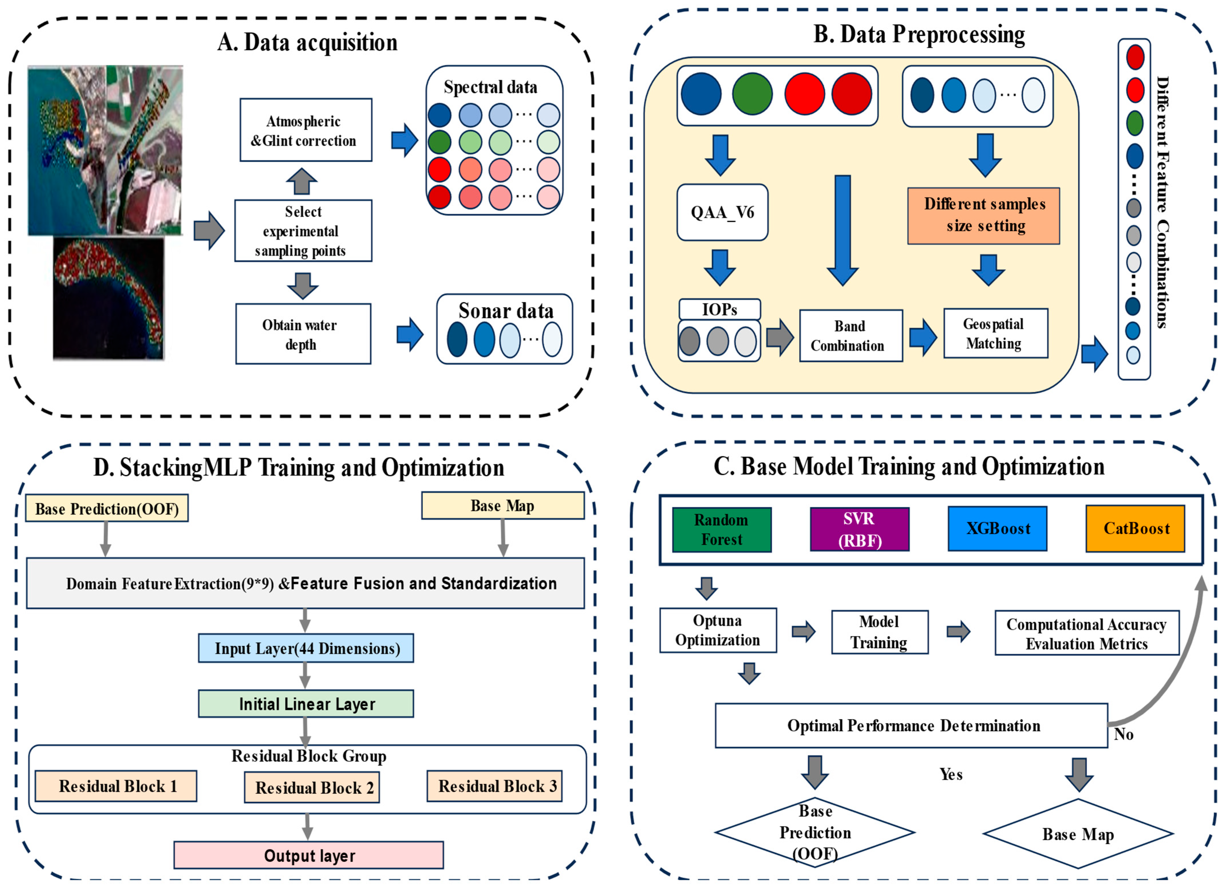
To address the dual challenges of physical ambiguity and spatial incoherence that characterize satellite-derived bathymetry (SDB), we designed and validated the OptiFusionStack framework. This hierarchical, two-stage “physio-spatial” architecture employs a ‘divide-and-conquer’ strategy. In the first stage, it decouples the raw remote sensing signal into preliminary depth predictions using physics-informed base learners. In the second stage, a meta-learner effectively fuses these predictions with rich spatial context to generate the final, high-fidelity bathymetric map.
The overall workflow, illustrated in Figure 2, is organized into four logical steps: (A) Data Acquisition and Preprocessing; (B) Physics-Informed Feature Engineering; (C) Stage 1 Base Learner Training, where an ensemble of diverse base learners generates preliminary prediction maps; and (D) Stage 2 Meta-Learner Fusion, where a StackingMLP meta-learner uses the outputs from Stage 1 along with multi-scale spatial statistics to produce the final prediction.
In essence, Stage 1 mitigates physical ambiguity by transforming the highly entangled spectral information into more reliable, decorrelated depth estimates. Stage 2, in turn, addresses spatial incoherence by leveraging geospatial patterns within a pixel’s neighborhood to correct artifacts, suppress noise, and enhance the geographical realism of the final product. With this overarching structure established, the subsequent sections will elaborate on each of these key modules.

2.3. Feature Engineering: A Two-Stage Physio-Spatial Approach

All analyses in this study utilized the Level-2A (L2A) surface reflectance ( R r s , s r 1 ) products from the Sentinel-2B satellite, provided through the Copernicus program. The L2A dataset is a standard product generated by the official Sen2Cor processor, which applies atmospheric correction to the initial Level-1C data. Consequently, the pixel values in the imagery already represent bottom-of-atmosphere (BOA) reflectance. This obviates the need for any additional atmospheric correction, allowing our feature engineering process to commence directly from this high-quality, pre-processed data.
The success of the proposed OptiFusionStack framework hinges on a sophisticated two-stage feature engineering strategy. This strategy is designed to synergistically integrate physical priors with spatial context, thereby transforming the entangled spectral signals of the L2A data into a decoupled, semantically rich feature set. By doing so, it addresses the dual challenges of physical ambiguity and spatial blindness inherent in satellite-derived bathymetry.
The foundational step of this framework moves beyond empirical spectral relationships to ground the analysis in optical physics. To this end, the Quasi-Analytical Algorithm (QAA) is employed to derive inherent optical properties (IOPs) and apparent optical properties (AOPs) from the Sentinel-2B L2A surface reflectance products. This process yields a focused set of physical priors at the 490 nm wavelength. These priors, which characterize the key optical state of the water column, serve to mitigate the confounding effects of water quality variability.
The implementation of the QAA commences with the conversion of the above-surface reflectance ( R r s ) to its sub-surface equivalent ( r r s ), as detailed in Formula 1. This sub-surface reflectance then serves as the foundational input for deriving the subsequent optical properties.
The algorithm first calculates an intermediate parameter, μ ( λ ) , according to Formula (2). This step utilizes the model coefficients g 0 (0.089) and g 1 (0.1245), which are based on the empirical relationship established by Lee et al. (2002) [24] for converting above-surface to sub-surface reflectance.
A key step follows: the empirical estimation of the total absorption coefficient at a reference wavelength of 560 nm, a ( 560 ) . This is achieved by first computing a logarithmic reflectance ratio, χ (Formula (3)), and then applying this ratio in the relationship described by Formula (4). The empirical coefficients h 0 , h 1 , and h 2 are set to −1.146, −1.366, and −0.469, respectively; these values were originally derived by Lee et al. (2002) [24] from extensive data fitting. With a ( 560 ) determined, the particulate backscattering coefficient, b b p ( 560 ) , is algebraically derived using Formula (5).
The spectral shape of particulate backscattering is then modeled as a power law. The exponent, η, is determined from the reflectance ratio between blue and green bands (Formula (6)), which in turn allows for the extrapolation of b b p   ( λ ) across the spectrum (Formula (7)). The total backscattering coefficient, b b   ( λ ) , is subsequently calculated as the sum of the particulate and pure water components (Formula (8)).
With the total absorption a ( λ ) determined, it is decomposed into its primary constituents: phytoplankton absorption ( a p h y ) and combined colored dissolved and detrital matter absorption ( a d g ). Specifically, a p h y ( 490 ) is isolated from the total absorption as described in Formula (9). The value for a d g ( 490 ) is then calculated via Formula (10), assuming a default spectral slope ( S ) of 0.015. This constant is a widely adopted value for the spectral slope in ocean optics and is recommended in standard QAA implementations (e.g., [21]).
Finally, the diffuse attenuation coefficient, K d ( 490 ) , is calculated using a semi-analytical model rooted in radiative transfer theory (Formula (11)). This model employs the semi-empirical constants κ and μ d , set to 1.1 and 0.54, respectively. The validity of this simplified radiative transfer approach has been demonstrated in numerous studies and applied in similar semi-analytical inversion algorithms (e.g., [13]).
This multi-step process ultimately generates three core physical prior features for each pixel: K d ( 490 )   a d g ( 490 ) , and a p h y ( 490 ) . These priors, combined with the original spectral bands, form the final physio-spectral data cube used for model input, as detailed in Table 1. To ensure spatial alignment, all bands within this data cube were resampled to a consistent 10-m resolution.
To overcome the “spatial blindness” inherent in traditional pixel-wise methods, the second stage of the feature engineering process is dedicated to constructing a rich set of spatial context features. This is achieved through a neighborhood feature extraction module that operates on the physio-spectral feature cube generated in the previous stage (as defined in Table 1).
For each sample point, instead of relying solely on its point-wise feature vector, a 9 × 9 pixel neighborhood window centered on the point is analyzed. The 9 × 9 window size was selected based on a sensitivity analysis, which demonstrated that this dimension provides an optimal balance between capturing meaningful geographic context and minimizing the risk of incorporating irrelevant distal information at the given data resolution.
Within this window, four key spatial statistics are computed for each of the N layers in the feature cube: mean, standard deviation (std), minimum (min), and maximum (max). This process transforms the initial point-wise feature vector into a comprehensive representation that encapsulates not only the point’s intrinsic properties but also the statistical characteristics of its immediate surroundings. The physical interpretation of these spatial features is crucial. Specifically, the mean provides a smoothed, robust estimate of local conditions; the standard deviation serves as a powerful descriptor of local heterogeneity, such as steep bathymetric gradients or water mass boundaries; and the min/max values capture the range of local variability. This context-rich feature set constitutes the final input for the model, enabling it to generate predictions that are both physically sound and spatially coherent.
r r s λ = R r s λ 0.52 + 1.7 R r s λ
u λ = g 0 + [ g 0 2 + 4 g 1 r rs λ ] 1 2 2 g 1
X = l o g 10 r r s 443 + r r s 490 r r s 560 + 5 ( r r s ( 670 ) 2 r r s ( 560 ) )
a λ 0 = a w λ 0 + 1 0 h 0 + h 1 χ + h 2 χ 2
b b p 560 = u 560 a 560 1 u 560 b b w 560
η = 2.0 1 1.2 exp 0.9 r r s 443 r r s 560
b b p λ = b b p 560 560 λ η
b b λ = b b p λ + b b w λ
a p h y ( 490 ) = a ( 490 ) a w ( 490 ) a d g ( 490 )
a d g ( 490 ) = a d g ( 560 ) e x p ( S ( 490 560 ) )
K d λ = a λ + κ b b ( λ ) μ d

Stage 2: Multi-Scale Spatial Context Construction

This spatial feature construction process generates a high-dimensional feature vector for each sample point. This vector encapsulates not only the point’s intrinsic properties but also the statistical characteristics of its immediate surroundings. The detailed composition of this final feature set, which serves as the input for the meta-learner, is presented in Table 2.
The specific feature composition is as follows: mean, standard deviation, minimum, and maximum statistics for 4 spectral bands and 3 IOPs (7bands total) within a 9 × 9 neighborhood window (7 × 4 = 28 dimensions), plus 4 statistics for 4 base model predictions within a 9 × 9 neighborhood window (4 × 4 = 16 dimensions), totaling 4 + 28 + 16 = 48 dimensions.
The physical interpretation of these spatial features is crucial. The mean provides a smoothed, robust estimate of local conditions. The standard deviation serves as a powerful descriptor of local heterogeneity, such as steep bathymetric gradients or water mass boundaries, offering invaluable information that is invisible to pixel-wise methods. The min/max values capture the range of local variability.
A notable architectural choice in this framework is the deliberate exclusion of the point-wise raw spectral and IOP features from the final meta-learner’s input. This decision is grounded in the core principle of the hierarchical, “divide-and-conquer” strategy. The Level 1 base models have already processed and distilled essential information from the raw point-wise features into their Out-of-Fold (OOF) predictions. These OOF predictions represent a higher-level, decorrelated, and effectively denoised abstraction of the initial data. Re-introducing the raw point-wise features at Level 2 would be redundant and risk re-injecting the multicollinearity and signal noise that the base learners were designed to mitigate. Conversely, the neighborhood statistics derived from the base model prediction maps are included because they provide a fundamentally different type of information: spatial context. This strategic choice ensures that the meta-learner receives a lean, powerful, and minimally redundant feature set. Each component thus provides a unique dimension of information—predictive (from OOFs) and contextual (from neighborhood statistics).

2.4. The OptiFusionStack Modeling Framework

Following the overall design presented in Section 2.2, this section details the construction, training, and synergistic mechanisms of the two-stage model integral to the OptiFusionStack framework.
A critical methodological consideration throughout the model training and evaluation was the strict adoption of a Spatial Block Cross-Validation strategy. This approach was chosen to ensure the validity of the results, as conventional random cross-validation can lead to a significant overestimation of a model’s true generalization capabilities due to “spatial leakage.”
To mitigate this risk, all samples within each study area were first partitioned into a regular 5 × 5 grid based on their geographic coordinates. Subsequently, during the 5-fold cross-validation process, entire columns of these geographic blocks were used as the basic units for data partitioning. This design enforces a strict geographical separation between the training and validation sets, thereby compelling the model to learn a generalizable mapping from spectral features to depth.

2.4.1. Level 1: Initial Prediction with Physics-Informed Base Learners

The foundation of the OptiFusionStack framework is an ensemble of four powerful and methodologically diverse machine learning models: Random Forest (RF), Support Vector Regression (SVR), XGBoost, and CatBoost. The primary function of these base learners is not to produce the final map, but rather to act as a diverse group of “initial interpreters.” Each model is independently trained on the physio-spectral feature cube (detailed in Section 2.3) to transform the noisy, raw input signals into a set of more meaningful and decorrelated preliminary depth predictions. This stage yields two key outputs that serve as high-quality inputs for Stage 2: (1) four full-coverage prediction maps, referred to as Base Maps, and (2) the corresponding point-wise Out-of-Fold (OOF) predictions.

2.4.2. Level 2: Synergistic Spatial Fusion with a StackingMLP Meta-Learner

The core innovation of the OptiFusionStack framework lies in its Level 2 meta-learner, an advanced StackingMLP. Unlike the base learners, the meta-learner utilizes a carefully constructed high-dimensional feature vector. This vector combines predictive information (the OOF predictions from Stage 1) with contextual information (the neighborhood statistics). This unique design enables the meta-learner to simultaneously consider “what” is predicted for a point and “where” that point is located, thereby functioning as both a “spatial regularizer” and an “intelligent arbiter.” The meta-learner learns to weigh the predictions from different base models and leverage spatial context to suppress noise and correct artifacts. Ultimately, this process yields a bathymetric product with spatial coherence and geographical realism far superior to what any single base model could achieve.

2.5. Accuracy Assessment Metrics

The performance of the bathymetry inversion models was quantitatively evaluated using four standard metrics to assess the agreement between model predictions ( y ^ i ) and in situ measurements ( y i ). The specific formulas for these metrics are provided in Equations (12)–(15), where ȳ represents the mean of in situ depths and n is the total number of samples.
The coefficient of determination (R2) measures the proportion of the variance in the in situ data that is predictable from the model. R2 ranges from 0 to 1, where a value closer to 1 indicates a better model fit.
The root mean squared error (RMSE) quantifies the average magnitude of the errors, expressed in the same units as the depth. Lower RMSE values signify higher accuracy. Because the error terms are squared before averaging, this metric is particularly sensitive to large deviations or outliers in the predictions.
The mean absolute error (MAE), in contrast, measures the average absolute difference between predicted and observed values. As it is less sensitive to outliers than RMSE, MAE provides a more robust assessment of the overall model performance.
Finally, the mean relative error (MRE) evaluates the average relative deviation, which is useful for comparing performance across depth ranges with significant magnitude differences. To prevent division by zero in the MRE calculation, any in situ depth ( y i ) of zero was replaced with a small epsilon value.
R 2 = 1 i = 1 n y i y ^ i 2 i = 1 n y i y 2
R M S E = 1 n i = 1 n   y i y ^ i 2
M A E = 1 n i = 1 n | y i y ^ i |
MRE = 1 N N i = 1 y ^ i y i y i

3. Results

3.1. Determination of Optimal Neighborhood Size

The scope of the spatial context, defined by the neighborhood window size, is a critical hyperparameter within the physio-spatial framework. A sensitivity analysis was conducted to identify the optimal neighborhood scale—one that effectively captures local geospatial correlations while avoiding the introduction of irrelevant noise. This analysis was performed on the Nanshan Port dataset using the OptiFusionStack framework, which was configured with its optimal combination of physical priors (i.e., K d and a d g ( 490 ) ), a choice validated later in this study. A range of neighborhood window sizes, from 3 × 3 to 11 × 11 pixels, was systematically evaluated.
As detailed in Table 3, the model’s performance exhibited a clear trend of improvement followed by stabilization as the neighborhood window size expanded. Specifically, as the window size increased from 3 × 3 to 9 × 9, all accuracy metrics showed significant enhancement: the R2 value rose from 0.9136 to 0.9176, while the RMSE decreased from 0.6151 m to 0.5818 m. This indicates that a broader scope of spatial information is crucial for correcting pixel-wise prediction biases. However, when the window was further enlarged to 11 × 11, no significant performance gain was observed; instead, a slight degradation occurred. This is likely because an overly large window begins to incorporate environmental noise from features that are not geospatially correlated with the central pixel.
Therefore, the 9 × 9 window was identified as the optimal neighborhood size, as it strikes the best balance between capturing sufficient spatial context and maintaining the local relevance of the extracted features. Consequently, all subsequent experiments in this study—including the base model performance evaluation and the benchmark against end-to-end models—utilize this optimized window size for spatial feature extraction.

3.2. Retrieval and Correlation Analysis of IOPs

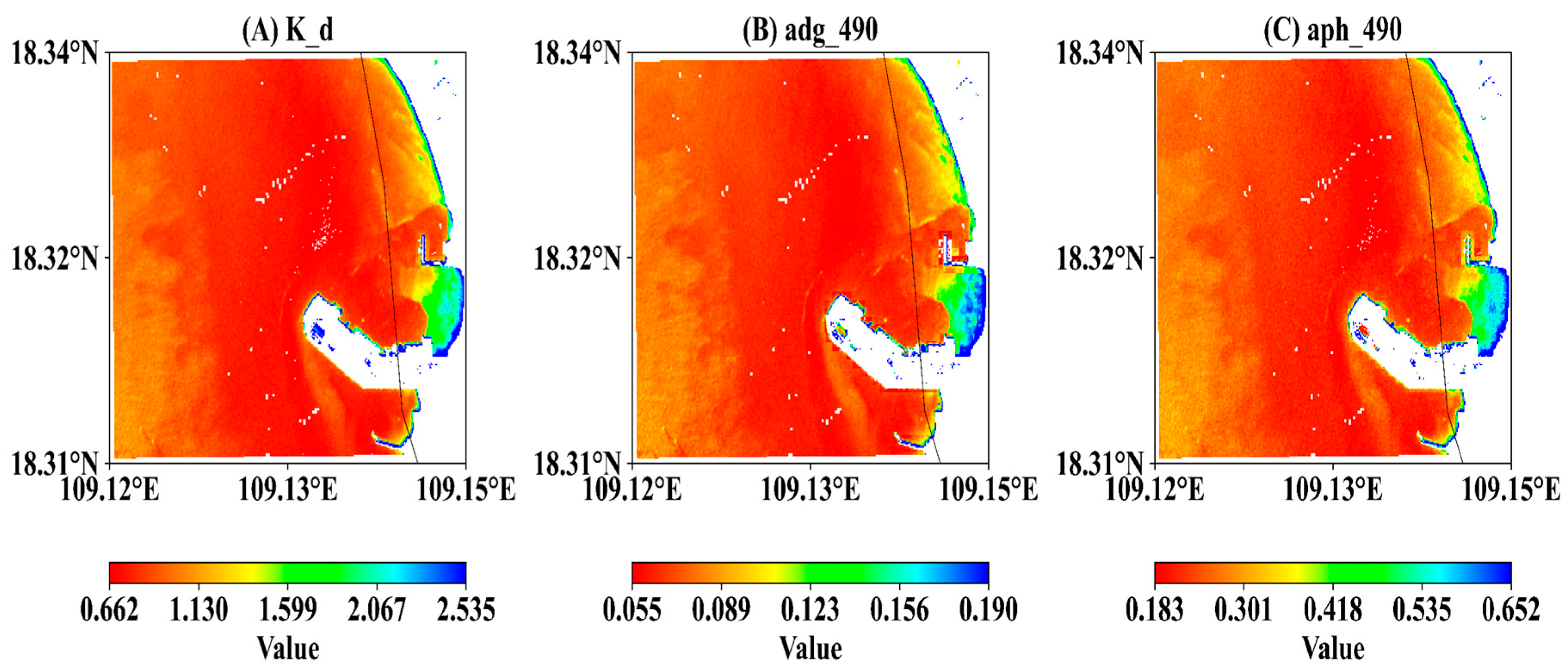
To ground the model in optical physics, key inherent optical properties (IOPs)—specifically, K d , a d g ( 490 ) , and a p h y ( 490 ) —were retrieved using the QAA_v6 algorithm. Their spatial distributions (Figure 3) align with known hydro-ecological dynamics, confirming their physical plausibility. However, a quantitative analysis reveals a critical challenge: as shown in Figure 4, all IOP pairs exhibit strong Pearson correlations (r > 0.91), indicating significant multicollinearity. This presents a classic physio-statistical dilemma: while physically meaningful, the statistical redundancy of these features implies that their naive inclusion may not substantially boost model performance. This inherent tension motivates the subsequent performance evaluation.
To further validate these uncalibrated physical priors, the diffuse attenuation coefficient, K d ( 490 ) , was compared against typical values from published literature (Table 4). K d ( 490 ) was selected because it is a key indicator that integrally represents the total attenuation properties of the water column, making its validation a macroscopic assessment of the entire IOP inversion chain’s plausibility.
The derived K d ( 490 ) values are highly consistent with physical expectations across the different water types. For the clear waters of the Qilian Islands, the derived range (0.046–0.33 m−1) approaches the theoretical limit for the clearest natural waters (0.02–0.15 m−1) reported by Hochberg (2003) [27]. In stark contrast, K d ( 490 ) values were substantially higher at Nanshan Port (0.662–2.535 m−1) and the Yellow River (1.587–5.152 m−1), ranges that are in excellent agreement with observations by Sokoletsky & Shen (2014) [19] and Qiu et al. (2013) [30] for turbid coastal and estuarine waters.
This comparative analysis provides strong evidence that, even without local calibration, the QAA model successfully captured the macroscopic differences in water optical properties among the study sites. It thereby supplied the subsequent machine learning models with physically plausible and directionally correct prior information, providing a solid foundation for the framework’s physics-informed strategy.

3.3. Performance Bottlenecks of Pixel-Wise Models

To evaluate the effect of adding physics-informed priors to standard pixel-wise models, four base learners were tested across eight feature combinations. The results, summarized in Figure 5, reveal a distinct performance plateau, thereby demonstrating the inherent limitations of this approach.
As shown in Figure 5, the naive fusion of QAA-derived IOPs with spectral data yields only marginal and inconsistent gains over the spectral-data-only baseline. Across all models, performance metrics remain confined to a narrow range (e.g., R2 values are largely below 0.67), failing to show a transformative benefit from the inclusion of these physical parameters. The tightly clustered and intersecting trend lines in the figure clearly indicate a “performance bottleneck.”
This performance stagnation highlights that pixel-wise models struggle to effectively utilize the rich, yet highly collinear, physical features. More importantly, these models are inherently incapable of modeling spatial context. This limitation powerfully motivates the need for the advanced, context-aware architecture proposed in this work.

3.4. Performance of OptiFusionStack Framework

In stark contrast to the performance plateau of the pixel-wise base models detailed in Section 3.3, the OptiFusionStack framework demonstrates a transformative leap in bathymetric accuracy. This improvement is achieved by synergistically integrating physical information with spatial context.

3.4.1. Global Performance Assessment and Optimal Feature Selection

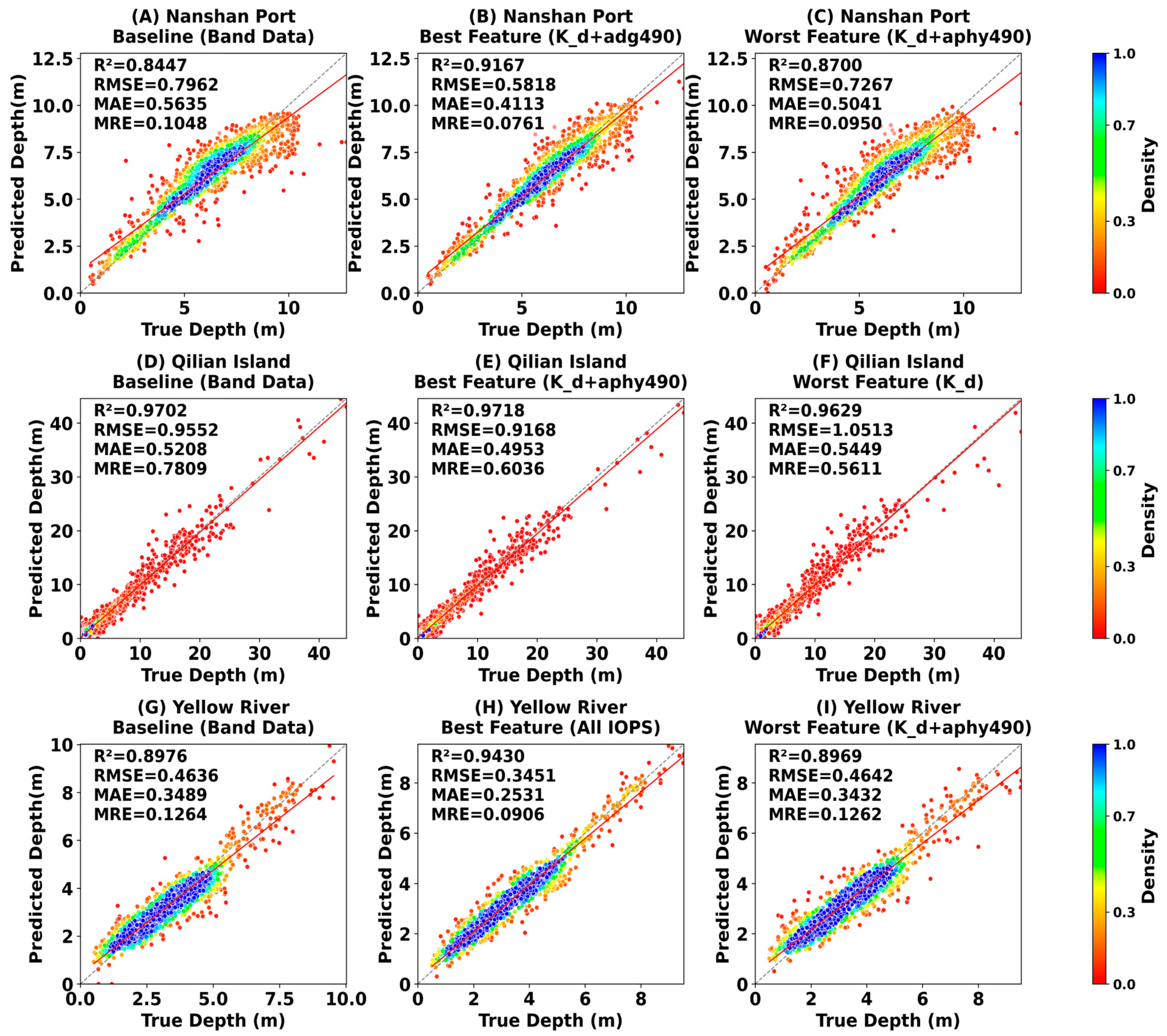
Figure 6 presents the validation scatter plots for the OptiFusionStack meta-learner, comparing the baseline (“Band Data only”) with the best- and worst-performing feature combinations across the three study areas. The results unequivocally highlight the framework’s superiority. At each site, the optimal feature combination decisively outperformed the baseline, evidenced by a much denser clustering of points around the 1:1 line and significant improvements in all performance metrics. For instance, at Nanshan Port (Figure 6A–C), the optimal configuration ( K d + a d g ( 490 ) ) elevated the R2 value from 0.8447 to 0.9167 and reduced the RMSE from 0.7962 m to 0.5818 m.
Interestingly, the optimal feature set was adaptive to the local optical environment. While a combination of K d and physical absorption priors ( a p h y ,   a d g ) was favored in the moderately to highly turbid waters of Nanshan Port and the Yellow River, spectral information alone remained highly effective in the clear waters of the Qilian Islands (Figure 6E,H). This adaptability demonstrates the framework’s ability to intelligently weigh different information sources based on environmental conditions. A complete set of scatter plots for all feature combinations is available in the Supplementary Materials (Figure S1) for a more exhaustive comparison.

3.4.2. Analysis of Robustness Across Depths and Environments

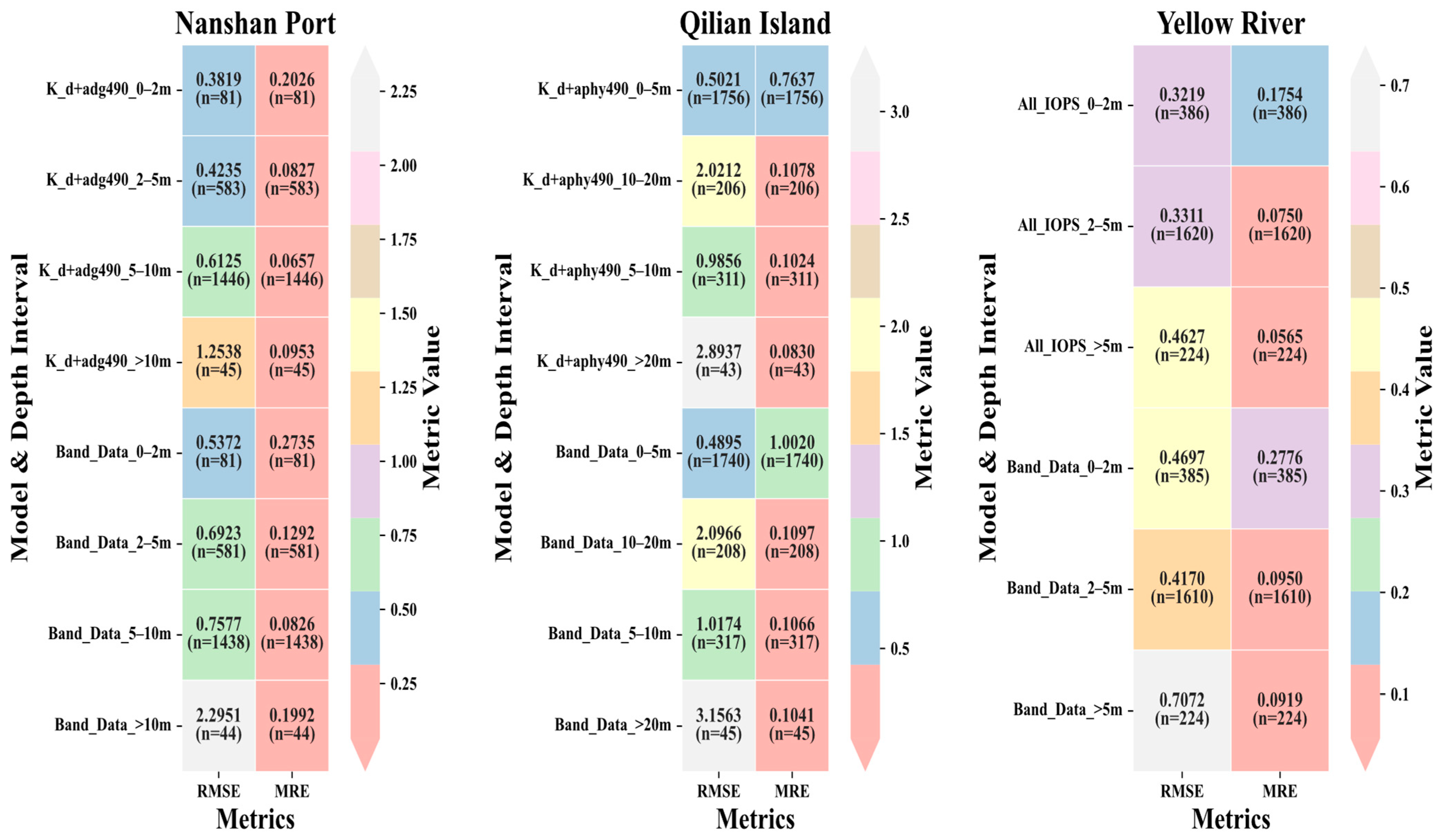
To investigate the framework’s stability beyond global metrics, a depth-stratified error analysis was conducted. Figure 7 presents heatmaps that compare the RMSE and MRE of the baseline and best-performing models within specific depth intervals for each study area.
This granular analysis reveals the underlying reasons for the framework’s superior performance. The heatmaps show that for nearly every depth bin, the optimal OptiFusionStack model yields a consistently lower RMSE and MRE than the baseline. This outperformance is particularly evident in the most challenging conditions. For instance, in the deeper waters of the Qilian Islands (>20 m), the optimal model reduced the MRE from over 30% to approximately 20% (Figure 7, middle panel). Similarly, in the optically complex and highly turbid shallow waters (<5 m) of the Yellow River, the optimal model maintained an RMSE below 0.35 m, significantly outperforming the baseline (Figure 7, right panel).
In summary, this depth-stratified analysis confirms that the performance enhancement offered by OptiFusionStack is not merely a global average but a consistent and robust improvement across diverse depth regimes and extreme optical environments. This analysis demonstrates the framework’s reliability and adaptability, making it a highly suitable candidate for operational SDB applications.

3.4.3. Superior Spatial Coherence and Artifact Suppression

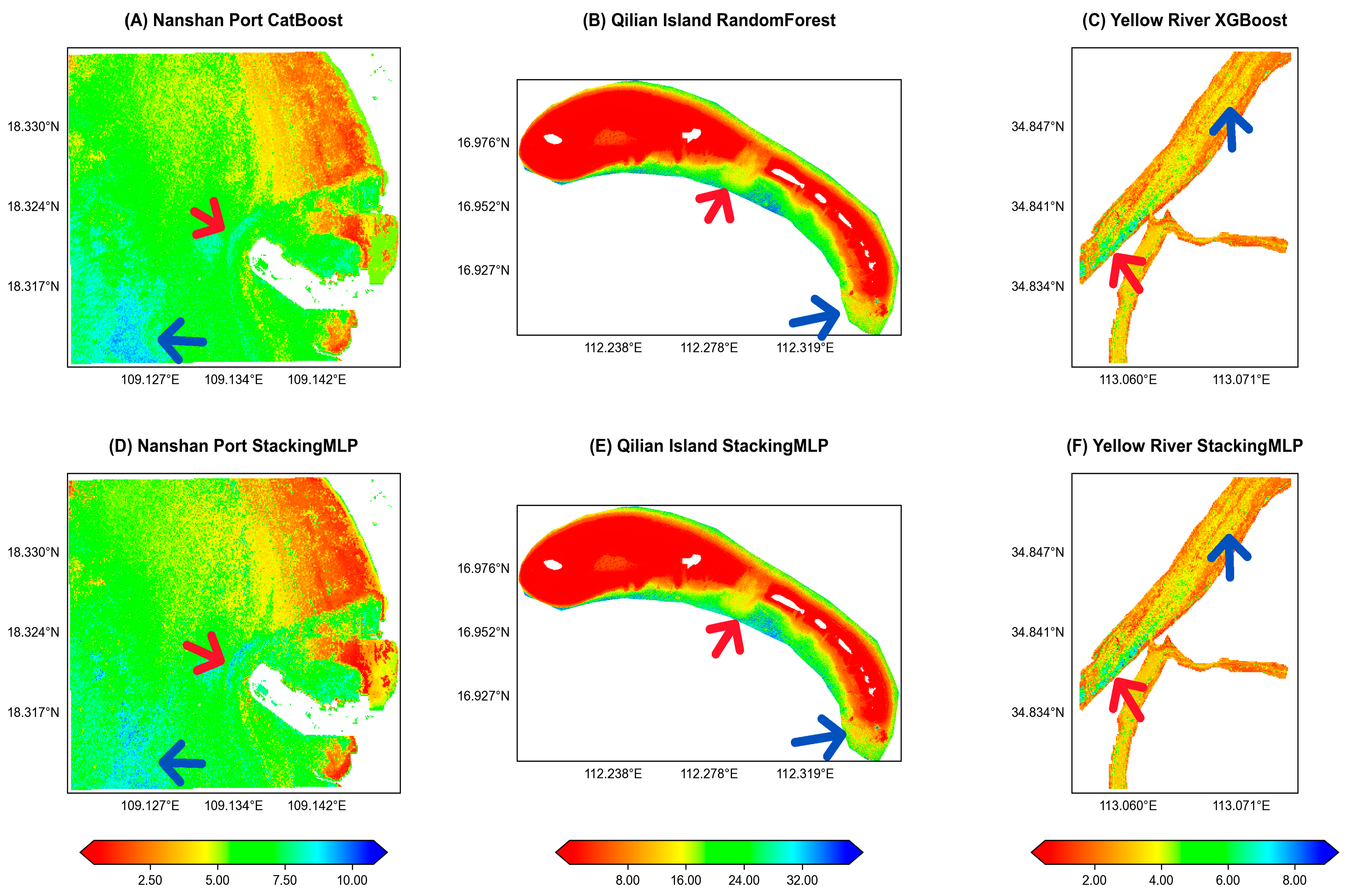
Beyond point-wise accuracy, a model’s utility is also determined by its spatial coherence. Figure 8 provides a compelling visual comparison between the optimal pixel-wise base model outputs (top row) and the results from the context-aware OptiFusionStack framework (bottom row).
The outputs of the base models are consistently plagued by spatial artifacts—such as noise, patchiness, and artificial edges (Figure 8A–C, red arrows)—which are a direct result of their inherent “spatial blindness.” In stark contrast, the OptiFusionStack framework (Figure 8D–F) rectifies these deficiencies. By acting as a powerful spatial regularizer, it produces markedly smoother and more geographically realistic bathymetric maps.
However, this regularization involves a trade-off, leading to a predictable limitation, as indicated by the blue arrows. The framework’s smoothing effect can blur fine-scale geomorphic features and underestimate sharp depth gradients (Figure 8D–F). This trade-off between noise suppression and fine-detail preservation is a key characteristic of the proposed approach, making it ideal for robust, landscape-scale mapping, though potentially less suitable for resolving sub-window-scale features.

3.4.4. Architectural Superiority: A Benchmark Against Monolithic Deep Learning Models

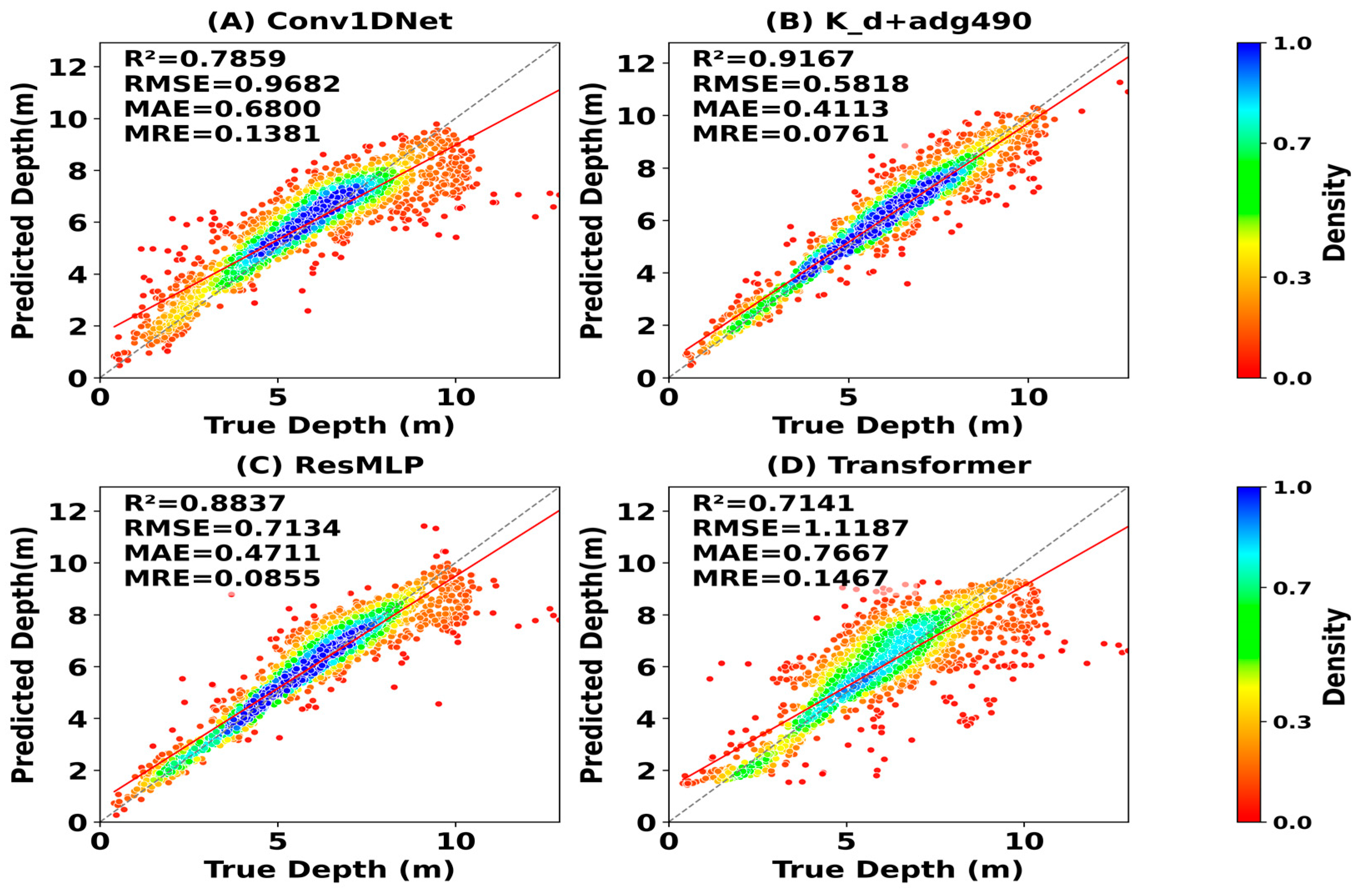
To validate the architectural advantage of the proposed hierarchical framework, a rigorous benchmark was conducted against three state-of-the-art, monolithic deep learning models optimized for tabular data: a CNN (Conv1DNet), an MLP (ResMLP), and a Transformer.
A scrupulously fair comparison was ensured by training all models, including the proposed OptiFusionStack, on the exact same optimal input feature set (i.e., spectral bands + K d + a d g ( 490 ) priors with 9 × 9 neighborhood statistics) and using identical training protocols. This experimental design isolates the architectural choice as the sole differentiating factor.
The results, presented in Figure 9, are unequivocal. The proposed OptiFusionStack framework (Figure 9B) achieved significantly higher accuracy (R2 = 0.9167, RMSE = 0.5818 m) than all benchmark models. Even the best-performing monolithic model, ResMLP (Figure 9C), lagged considerably behind (R2 = 0.8837, RMSE = 0.7134 m), while the CNN and Transformer performed even worse, exhibiting greater scatter and higher errors.
This outcome provides compelling evidence for the superiority of the “divide-and-conquer” strategy. Instead of tasking a single, large network with the difficult job of learning from raw, noisy data, the proposed two-stage approach proves more effective. In this approach, base learners first denoise and abstract the information, and a meta-learner then fuses these refined predictions with spatial context. This hierarchical process is a more effective and accurate paradigm for this complex inversion task.

4. Discussion

4.1. The Physio-Spatial Synergy: From Signal Entanglement to Semantic Decoupling

The superior performance of the OptiFusionStack framework is not an incidental outcome of architectural complexity, but rather the result of a deliberate, two-pronged strategy. This strategy is designed to address the fundamental challenges of remote sensing inversion: physical ambiguity and spatial blindness. This section delves into the synergistic mechanisms by which this framework transforms a raw, entangled signal problem into a decoupled, semantically rich learning task.
Before delving into the analysis, a critical methodological consideration that underpins the validity of the results must be highlighted: the strict use of a spatial cross-validation strategy based on geographic blocking. Unlike conventional random pixel-wise sampling, the Out-of-Fold (OOF) predictions in this study were generated by training and validating on geographically disjoint data blocks. This choice is paramount for a valid assessment of model generalizability, as conventional random splitting can lead to significant overestimation of model performance due to “spatial leakage”—a phenomenon where highly correlated, neighboring pixels are present in both the training and validation sets. The implemented spatial cross-validation strategy prevents this risk, ensuring that the final model’s evaluation genuinely reflects its ability to generalize to unseen geographic locations (i.e., for spatial extrapolation). This methodological rigor provides a robust foundation for all subsequent discussions.

4.1.1. The Role of IOPs: Decoupling the Physical Signal

The first critical step in the proposed framework is the decoupling of the physical signal, a process visually diagnosed in Figure 10. When using only raw spectral bands, the relationship between spectral values and water depth is highly entangled, non-linear, and ambiguous (Figure 10B). The signal recorded by the satellite is a convoluted mixture of depth-dependent attenuation, bottom reflectance, and variable absorption and scattering from water constituents. Learning a robust function from this entangled signal space is an ill-posed problem for any model, which explains the performance bottlenecks observed in the base models.
The introduction of IOPs, however, fundamentally reframes this problem as a process of feature reconstruction rather than mere addition. By converting apparent reflectance into intrinsic optical properties, a coherent physical logic chain is established. As illustrated by combinations such as “ a d g ( 490 )   +   a p h y ( 490 ) ” (Figure 10F), the explicit quantification of absorption from non-algal particles ( a d g ) and phytoplankton ( a p h y ) decontaminates the spectral signals. This allows the model to better isolate depth-dependent attenuation, thereby stabilizing the spectral response. In essence, IOPs act as a key to unlock the physical processes encoded within the signal. They transform the problem from “correlating mixed signals to depth” to “modeling depth from decoupled physical constituents,” providing a more robust and mechanistically grounded foundation for learning.

4.1.2. The Role of Spatial Context: Decoupling the Geographic Semantics

While IOPs address the “what” (the physical meaning of a point), they do not address the “where” (its geographic context). This constitutes the second crucial stage of decoupling, performed by the neighborhood feature extraction module. A pixel in isolation is merely a vector of numbers; within its neighborhood, however, it acquires geographic semantics.
The neighborhood statistics, particularly the standard deviation, are not merely statistical measures but also proxies for geomorphological and hydrological features. For instance, a low standard deviation on the K d map signifies a “region of optically uniform water,” whereas a high standard deviation indicates a “steep gradient of water clarity” or a “frontal zone.” Similarly, a high standard deviation on a base model’s prediction map signifies a “region of high bathymetric relief” or a “potential reef edge.”
By feeding these semantically rich spatial features to the meta-learner, the learning task is elevated beyond simple pixel-wise regression. The model becomes a context-aware reasoner, capable of answering complex questions, such as: “Given that this point has the optical properties of clear water (from IOPs) and is located in a region of very low bathymetric relief (from the low neighborhood std of base predictions), what is its most likely depth?” This ability to synergistically fuse the decoupled physical signal with geographic semantics is the core reason for the framework’s success. This fusion allows the model to produce predictions that are not only physically plausible at a point level but also geographically consistent at a landscape scale—a feat unattainable by models that address only one of these challenges in isolation.

4.2. Advantages of the Stacking Framework: Architectural Intelligence and Information Prioritization

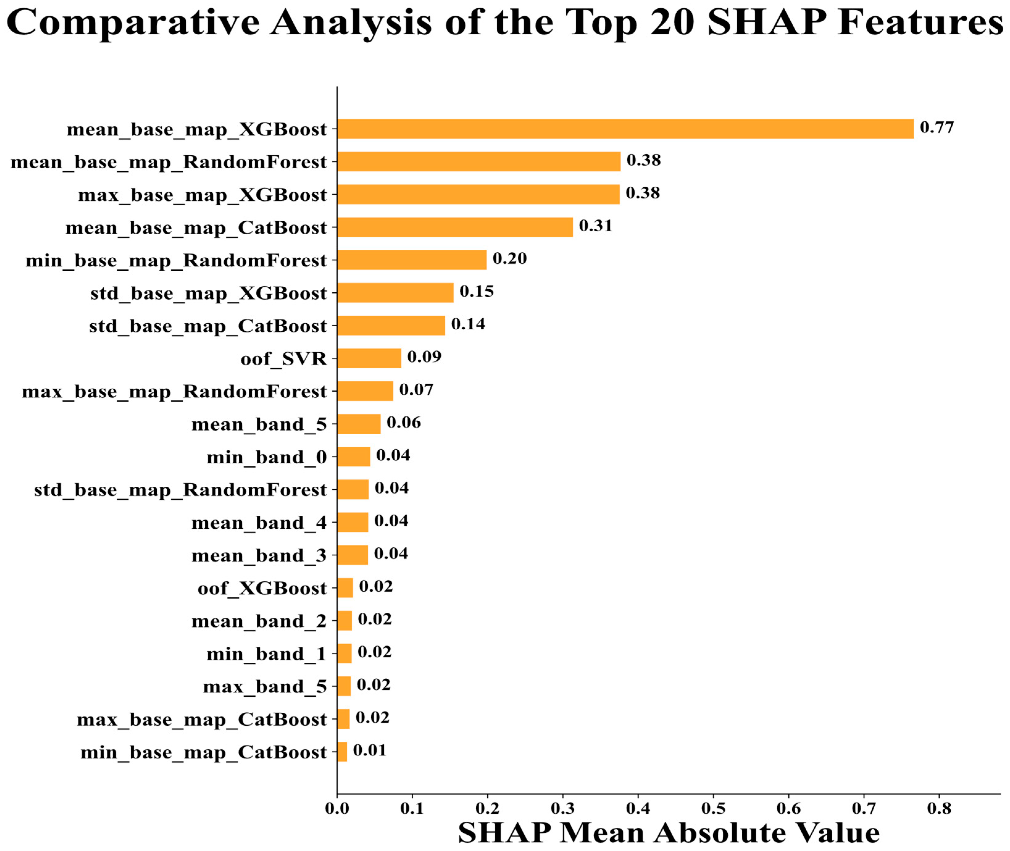
The success of the OptiFusionStack framework is not merely a product of feature enrichment, but of its architectural intelligence in navigating and prioritizing a complex, multi-scale feature set. To deconstruct the meta-learner’s decision-making process, a SHAP (SHapley Additive exPlanations) analysis was conducted. This section focuses on the optimal K d + a d g ( 490 )   configuration to elucidate the core mechanisms. As presented in Figure 11, the mean absolute SHAP values for the top 20 features provide quantitative evidence of the framework’s synergistic fusion mechanism and reveal a clear hierarchy of information importance.
The analytical approach was as follows: given the complexity of the StackingMLP meta-learner, the model-agnostic KernelExplainer from the shap library was utilized. To balance computational efficiency with representativeness, a background dataset was created by randomly sampling 100 data points from the training set. SHAP values were then computed for a subset of 500 samples drawn from the test set. A robust ranking of global feature importance was then derived by calculating the mean absolute SHAP value for each feature across all explanation samples.

4.2.1. The Primacy of Spatial Context

The most striking finding from the SHAP analysis is the overwhelming importance of the neighborhood-derived spatial context features. As Figure 11 clearly illustrates, features such as mean_base_map_XGBoost (0.77), mean_base_map_RandomForest (0.38), and max_base_map_XGBoost (0.38) dominate the feature importance ranking. These features, which describe the average or maximum predicted depth in a pixel’s vicinity, contribute far more to the final prediction than any point-wise feature. This quantitatively confirms the central thesis of our study: spatial context is the primary driver of high-fidelity bathymetric mapping. By learning to rely on the smoothed, spatially-aware information from the neighborhood, the meta-learner effectively suppresses the noise and artifacts inherent in pixel-wise predictions, ensuring the spatial coherence of the final output. The high importance of statistics derived from multiple base model maps (e.g., XGBoost, RandomForest, CatBoost) also validates our ensemble approach, as the meta-learner leverages the diverse spatial perspectives provided by each base learner.

4.2.2. The Complementary Roles of Predictive and Physical Features

While spatial context forms the backbone of the prediction, the SHAP analysis also illuminates the complementary roles of point-wise predictive and raw physical/spectral features. The Out-of-Fold (OOF) prediction from SVR (oof_SVR, 0.09) emerges as the most important point-wise feature, demonstrating that the direct, abstracted outputs from the base models still provide crucial information for fine-tuning the final prediction at a specific location.
Furthermore, raw feature statistics, such as mean_band_5 (0.06), also retain importance. This indicates that even after information has been processed by the base learners, the meta-learner can still extract residual value directly from the original data layers to make final adjustments. In essence, the OptiFusionStack framework employs a sophisticated, multi-level decision-making process: it first establishes a robust, spatially consistent estimate based on neighborhood context; it then refines this estimate using the abstracted point-wise predictions from the base models; and finally, it makes subtle corrections based on the raw underlying physical/spectral data. This intelligent prioritization and fusion of information at different scales and levels of abstraction is the key to the framework’s architectural advantage and superior performance.

4.3. Architectural Considerations: Comparison with Convolutional Neural Networks (CNNs)

The proposed framework’s “neighborhood statistics + MLP” approach might, at first glance, appear structurally analogous to a simple Convolutional Neural Network (CNN). However, fundamental differences exist in their core design philosophies and operational mechanics.
First, the nature of feature generation is entirely different. In the proposed framework, the 9 × 9 neighborhood window is used to extract a set of pre-defined, handcrafted statistical features with clear physical interpretations (e.g., mean, standard deviation). In contrast, a CNN extracts features using learned convolution kernels, which typically represent abstract, data-driven patterns whose specific physical meaning is often uninterpretable.
Second, the proposed framework lacks a weight-sharing mechanism. Its neighborhood statistics are calculated through fixed mathematical operations that are applied consistently across the entire image. In contrast, weight sharing—a cornerstone of CNNs—allows the same kernel (a set of weights) to detect a pattern regardless of its location, thereby ensuring translational invariance and high parameter efficiency.
Finally, and most critically, OptiFusionStack is a decoupled, two-stage architecture, not an end-to-end model. Its Stage 1 base learners and Stage 2 meta-learner are trained sequentially; consequently, gradients from the meta-learner are not back-propagated to the base learners. A CNN, in contrast, is an end-to-end system where the gradient from the loss function flows through the entire network to update all weights simultaneously.
These distinctions are not incidental but are central to the “divide-and-conquer” strategy. This structured and interpretable approach was deliberately chosen to first denoise and interpret the signal physically (Stage 1), and then to focus on the fusion and regularization of spatial patterns (Stage 2). This step-wise problem-solving paradigm proved highly effective for the bathymetric inversion task at hand.

4.4. Implications, Limitations, and Future Directions Under Uncalibrated Conditions

Despite the robust performance of the OptiFusionStack framework, a clear acknowledgment of its limitations is crucial for driving future progress in the field. These challenges are concentrated in two main areas: the uncertainty of the input priors and the static nature of the spatial context modeling.
The first primary challenge stems from the uncertainty inherent in the input priors. On one hand, the framework’s accuracy is fundamentally capped by the performance of the uncalibrated upstream QAA model; while the architecture can correct for some deviations, it cannot eliminate systematic errors originating from the physical model itself. On the other hand, the temporal mismatch between some satellite images and the in situ bathymetric data introduces unquantifiable uncertainty into the ground-truth labels. Although the rigorous spatial block cross-validation strategy ensures a reliable assessment of model generalization, it cannot account for real-world bathymetric changes over time.
A second challenge involves the static nature of the spatial context modeling and its inherent trade-offs. The fixed 9×9 neighborhood window used in this study represents a compromise between capturing sufficient context and introducing irrelevant noise. This “one-size-fits-all” approach, however, may not be optimal for all geomorphic environments, such as gentle deltas versus steep reef crests. More importantly, any method based on neighborhood smoothing faces an intrinsic cost: while it effectively suppresses noise and artifacts to improve spatial coherence, it may also smooth over fine-scale, real-world seabed features.
These challenges also illuminate clear and exciting directions for future research.
One direction is moving towards more robust and dynamic physio-spatial learning. To enhance the quality of physical priors, sparse, high-accuracy data from sources such as ICESat-2 could be integrated for a “minimally-supervised” calibration of the QAA. To overcome the limitations of static spatial modeling, future architectures could incorporate adaptive neighborhoods or multi-scale fusion capabilities, potentially evolving into end-to-end networks like U-Net that can implicitly learn both physical relationships and dynamic spatial context within a unified framework.
Another direction is expanding from a single task to integrated monitoring applications. The framework’s core strength—its ability to learn effective patterns from imperfect physical parameters—opens a pathway to multi-target inversion. Future models could be designed to simultaneously retrieve bathymetry and relative water quality indicators (e.g., turbidity or chlorophyll concentration), thereby providing a powerful, cost-effective tool for the integrated and dynamic monitoring of coastal environments.

5. Conclusions

This study addressed the dual challenges of physical ambiguity and spatial blindness that have traditionally limited the accuracy and fidelity of satellite-derived bathymetry (SDB). A novel, two-stage physio-spatial framework, OptiFusionStack, was proposed and validated. This framework is designed to synergistically integrate physical priors with spatial context, crucially, under conditions where no in situ data is available for optical model calibration.
The findings reveal that the naive, pixel-wise fusion of uncalibrated, QAA-derived inherent optical properties (IOPs) with standard machine learning models yields only marginal performance gains, resulting in a performance plateau and spatially incoherent maps riddled with artifacts. The OptiFusionStack framework, however, decisively overcomes these limitations. By employing a hierarchical architecture—one that uses physics-informed base models to generate initial predictions and then feeds their multi-scale neighborhood statistics into a meta-learner—the framework achieves state-of-the-art performance. This is demonstrated by its outstanding accuracy (e.g., R2 > 0.92 in optically complex inland waters) and its ability to generate maps with superior spatial coherence.
Crucially, this research confirmed the mechanisms behind this success through rigorous validation. A SHAP analysis verified the framework’s decision-making logic, showing that it intelligently prioritizes spatial context as the primary driver for its predictions while using point-wise predictive and physical features for refinement. Furthermore, a rigorous benchmark against state-of-the-art deep learning models, including ResMLP and Transformer, demonstrated that the proposed hierarchical fusion paradigm is significantly superior in terms of accuracy, even when all models were provided with the same optimal feature inputs.
In conclusion, this research provides compelling evidence that the future of high-fidelity remote sensing inversion lies in the synergistic fusion of physical mechanisms with spatial context. The physio-spatial paradigm presented here offers a robust solution for producing geospatial products that are not just accurate but also geographically realistic, particularly in the challenging, data-scarce environments common in real-world applications.

Supplementary Materials

The following supporting information can be downloaded at: https://www.mdpi.com/article/10.3390/rs17223712/s1, Figure S1: The main content of the supplemental image is a scatterplot of the accuracy under multiple combinations of features for all study areas.

Author Contributions

Z.W. and J.L.: conceptualization, methodology, data curation, writing—original draft, writing—review and editing, and visualization. X.L.: Project administration. D.Z.: Supervision; Visualization. Z.W. and J.L.: conceptualization, methodology, writing, review and editing. W.S.: writing—review and editing, and supervision. Y.X.: Writing—original draft; All authors have read and agreed to the published version of the manuscript.

Funding

This work was supported by the 2023 Hainan Province “South China Sea New Star” Science and Technology Innovation Talent Platform Project (NHXXRCXM202316); in part by Hainan Natural Science Foundation of China (nos. 424QN253 and 620RC602); by the National Natural Science Foundation of China (no. 61966013); in part by the Teaching Reform Research Project, Hainan Normal University, hsjg2023-07; in part by the National Natural Science Foundation of China under grant 61991454; in part by the National Key Research and Development Program of China under grant 2023YFC3107605; in part by the Oceanic Interdisciplinary Program of Shanghai Jiao Tong University under grant SL2022ZD206; and in part by the Scientific Research Fund of Second Institute of Oceanography, MNR under grant SL2302.

Data Availability Statement

The Sentinel-2 Level-2A satellite imagery used in this study is publicly available from the Copernicus Data Space Ecosystem. The complete Python code to reproduce all analysis methods presented in this study has been deposited in a GitHub repository and is accessible at https://github.com/markeable/LjzBatchmtery.git (accessed on 9 November 2025). The in situ bathymetry datasets used in this study are not publicly available due to data sharing agreements but can be made available by the corresponding author upon reasonable request.

Acknowledgments

Special thanks to the Copernicus Data Space Ecosystem for providing the Sentinel-2 series products. During the preparation of this manuscript, the authors utilized the ChatGPT-5 language model from OpenAI for language editing, refinement, and correction of tense issues. The authors have reviewed and edited its output and assumes full responsibility for the content of this publication.

Conflicts of Interest

The authors declare no conflicts of interest.

References

  1. Caballero, I.; Stumpf, R.P. Retrieval of nearshore bathymetry from Sentinel-2A and 2B satellites in South Florida coastal waters. Estuar. Coast. Shelf Sci. 2019, 226, 106277. [Google Scholar] [CrossRef]
  2. Fang, S.; Wu, Z.; Wu, S.; Chen, Z.; Shen, W.; Mao, Z. Enhancing Water depth inversion accuracy in turbid coastal environments using random forest and coordinate attention mechanisms. Front. Mar. Sci. 2024, 11, 1471695. [Google Scholar] [CrossRef]
  3. Huang, W.; Zhao, J.; Ai, B.; Sun, S.; Yan, N. Bathymetry and benthic habitat mapping in shallow waters from Sentinel-2A imagery: A case study in Xisha islands, China. IEEE Trans. Geosci. Remote Sens. 2022, 60, 1–12. [Google Scholar] [CrossRef]
  4. Hedley, J.D. Remote sensing of coral reefs for monitoring and management: A review. Remote Sens. 2016, 8, 118. [Google Scholar] [CrossRef]
  5. Hedley, J.D.; Harborne, A.R.; Mumby, P.J. Technical note: Simple and robust removal of sun glint for mapping shallow-water benthos. Int. J. Remote Sens. 2005, 26, 2107–2112. [Google Scholar] [CrossRef]
  6. Li, J.; Chu, S.; Hu, Q.; Qu, Z.; Zhang, J.; Cheng, L. A Slope Adaptive Bathymetric Method by Integrating ICESat-2 ATL03 Data with Sentinel-2 Images. Remote Sens. 2025, 17, 3019. [Google Scholar] [CrossRef]
  7. Kalybekova, A. A Review of Advancements and Applications of Satellite-Derived Bathymetry. Eng. Sci. 2025, 35, 1541. [Google Scholar] [CrossRef]
  8. Zhang, Y.; Liu, J.; Shen, W. A Review of Ensemble Learning Algorithms Used in Remote Sensing Applications. Appl. Sci. 2022, 12, 8654. [Google Scholar] [CrossRef]
  9. Wang, E.; Zhang, H.; Wang, J.; Cao, W.; Li, D. Simulation and Sensitivity Analysis of Remote Sensing Reflectance for Optically Shallow Water Bathymetry. Remote Sens. 2025, 17, 1384. [Google Scholar] [CrossRef]
  10. Pacheco, A.; Horta, J.; Loureiro, C.; Ferreira, Ó. Retrieval of nearshore bathymetry from Landsat 8 images: A tool for coastal monitoring in shallow waters. Remote Sens. Environ. 2015, 159, 102–116. [Google Scholar] [CrossRef]
  11. Xu, Y.; Cao, B.; Deng, R.; Cao, B.; Liu, H.; Li, J. Bathymetry over broad geographic areas using optical high-spatial-resolution satellite remote sensing without in-situ data. Int. J. Appl. Earth Obs. Geoinf. 2023, 119, 103308. [Google Scholar] [CrossRef]
  12. Zhang, X.; Chen, Y.; Le, Y.; Zhang, D.; Yan, Q.; Dong, Y.; Han, W.; Wang, L. Nearshore bathymetry based on ICESat-2 and multispectral images: Comparison between Sentinel-2, Landsat-8, and testing Gaofen-2. IEEE J. Sel. Top. Appl. Earth Obs. Remote Sens. 2022, 15, 2449–2462. [Google Scholar] [CrossRef]
  13. Zhong, J.; Sun, J.; Lai, Z.; Song, Y. Nearshore Bathymetry from ICESat-2 LiDAR and Sentinel-2 Imagery Datasets Using Deep Learning Approach. Remote Sens. 2022, 14, 4229. [Google Scholar] [CrossRef]
  14. Najar, M.A.; Benshila, R.; Bennioui, Y.E.; Thoumyre, G.; Almar, R.; Bergsma, E.W.J.; Delvit, J.-M.; Wilson, D.G. Coastal Bathymetry Estimation from Sentinel-2 Satellite Imagery: Comparing Deep Learning and Physics-Based Approaches. Remote Sens. 2022, 14, 1196. [Google Scholar] [CrossRef]
  15. Traganos, D.; Poursanidis, D.; Aggarwal, B.; Chrysoulakis, N.; Reinartz, P. Estimating Satellite-Derived Bathymetry (SDB) with the Google Earth Engine and Sentinel-2. Remote Sens. 2018, 10, 859. [Google Scholar] [CrossRef]
  16. He, C.; Jiang, Q.; Wang, P. An Improved Physics-Based Dual-Band Model for Satellite-Derived Bathymetry Using SuperDove Imagery. Remote Sens. 2024, 16, 3801. [Google Scholar] [CrossRef]
  17. Le, Y.; Sun, X.; Chen, Y.; Zhang, D.; Wu, L.; Liu, H.; Hu, M. High-accuracy shallow-water bathymetric method including reliability evaluation based on Sentinel-2 time-series images and ICESat-2 data. Front. Mar. Sci. 2024, 11, 1470859. [Google Scholar] [CrossRef]
  18. Lyzenga, D.R. Passive remote sensing techniques for mapping water depth and bottom features. Appl. Opt. 1978, 17, 379–383. [Google Scholar] [CrossRef]
  19. Sokoletsky, L.G.; Shen, F. Optical closure for remote-sensing reflectance based on accurate radiative transfer approximations: The case of the Changjiang (Yangtze) River Estuary and its adjacent coastal area, China. Int. J. Remote Sens. 2014, 35, 4193–4224. [Google Scholar] [CrossRef]
  20. Huang, E.; Chen, B.; Luo, K.; Chen, S. Effect of the One-to-Many Relationship between the Depth and Spectral Profile on Shallow Water Depth Inversion Based on Sentinel-2 Data. Remote Sens. 2024, 16, 1759. [Google Scholar] [CrossRef]
  21. Hsu, H.-J.; Huang, C.-Y.; Jasinski, M.; Li, Y.; Gao, H.; Yamanokuchi, T.; Wang, C.-G.; Chang, T.-M.; Ren, H.; Kuo, C.-Y.; et al. A semi-empirical scheme for bathymetric mapping in shallow water by ICESat-2 and Sentinel-2: A case study in the South China Sea. ISPRS J. Photogramm. Remote Sens. 2021, 178, 1–19. [Google Scholar] [CrossRef]
  22. Dorogush, A.V.; Ershov, V.; Gulin, A. CatBoost: Gradient boosting with categorical features support. arXiv 2018, arXiv:1810.11363. [Google Scholar] [CrossRef]
  23. McKinna, L.I.; Fearns, P.R.; Weeks, S.J.; Werdell, P.J.; Reichstetter, M.; Franz, B.A.; Shea, D.M.; Feldman, G.C. A semianalytical ocean color inversion algorithm with explicit water column depth and substrate reflectance parameterization. J. Geophys. Res. Oceans 2015, 120, 1741–1770. [Google Scholar] [CrossRef]
  24. Lee, Z.; Carder, K.L.; Arnone, R.A. Deriving inherent optical properties from water color: A multiband quasi-analytical algorithm for optically deep waters. Appl. Opt. 2002, 41, 5755–5772. [Google Scholar] [CrossRef]
  25. Zhang, X.; Ma, Y.; Zhang, J. Shallow Water Bathymetry Based on Inherent Optical Properties Using High Spatial Resolution Multispectral Imagery. Remote Sens. 2020, 12, 3027. [Google Scholar] [CrossRef]
  26. Saeidi, V.; Seydi, S.T.; Kalantar, B.; Ueda, N.; Tajfirooz, B.; Shabani, F. Water depth estimation from Sentinel-2 imagery using advanced machine learning methods and explainable artificial intelligence. Geomat. Nat. Hazards Risk 2023, 14, 2225691. [Google Scholar] [CrossRef]
  27. Hochberg, E.J.; Atkinson, M.J.; Andréfouët, S. Spectral reflectance of coral reef bottom-types worldwide and implications for coral reef remote sensing. Remote Sens. Environ. 2003, 85, 159–173. [Google Scholar] [CrossRef]
  28. Huang, R.; Yu, K.; Wang, Y.; Wang, J.; Mu, L.; Wang, W. Bathymetry of the Coral Reefs of Weizhou Island Based on Multispectral Satellite Images. Remote Sens. 2017, 9, 750. [Google Scholar] [CrossRef]
  29. Wu, Z.; Mao, Z.; Shen, W.; Yuan, D.; Zhang, X.; Huang, H. Satellite-derived bathymetry based on machine learning models and an updated quasi-analytical algorithm approach. Opt. Express 2022, 30, 16773–16793. [Google Scholar] [CrossRef]
  30. Qiu, Z.F.; Wu, T.T.; Su, Y.Y. Retrieval of diffuse attenuation coefficient in the China seas from surface reflectance. Opt. Express 2013, 21, 15287–15297. [Google Scholar] [CrossRef]
  31. Chen, T.; Guestrin, C. XGBoost: A Scalable Tree Boosting System. In Proceedings of the 22nd ACM SIGKDD International Conference on Knowledge Discovery and Data Mining, San Francisco, CA, USA, 13–17 August 2016; pp. 785–794. [Google Scholar] [CrossRef]
  32. Rehm, E.; McCormick, N.J. Inherent optical property estimation in deep waters. Opt. Express 2011, 19, 24986–25005. [Google Scholar] [CrossRef]
  33. Breiman, L. Random forests. Mach. Learn. 2001, 45, 5–32. [Google Scholar] [CrossRef]
  34. Zhu, X.X.; Tuia, D.; Mou, L.; Xia, G.-S.; Zhang, L.; Xu, F.; Fraundorfer, F. Deep Learning in Remote Sensing: A Comprehensive Review and List of Resources. IEEE Geosci. Remote Sens. Mag. 2017, 5, 8–36. [Google Scholar] [CrossRef]
  35. Kwon, J.; Shin, H.; Kim, D.; Lee, H.; Bouk, J.; Kim, J.; Kim, T. Estimation of shallow bathymetry using Sentinel-2 satellite data and random forest machine learning: A case study for Cheonsuman, Hallim, and Samcheok Coastal Seas. J. Appl. Remote Sens. 2024, 18, 014522. [Google Scholar] [CrossRef]
  36. Eugenio, F.; Marcello, J.; Mederos-Barrera, A.; Marqués, F. High-Resolution Satellite Bathymetry Mapping: Regression and Machine Learning-Based Approaches. IEEE Trans. Geosci. Remote Sens. 2022, 60, 1–14. [Google Scholar] [CrossRef]
  37. Liang, Y.; Cheng, Z.; Du, Y.; Song, D.; You, Z. An improved method for water depth mapping in turbid waters based on a machine learning model. Estuar. Coast. Shelf Sci. 2024, 296, 108577. [Google Scholar] [CrossRef]
  38. Wu, Z.; Zhao, Y.; Wu, S.; Chen, H.; Song, C.; Mao, Z.; Shen, W. Satellite-Derived Bathymetry Using a Fast Feature Cascade Learning Model in Turbid Coastal Waters. J. Remote Sens. 2024, 4, 0272. [Google Scholar] [CrossRef]
  39. Cheng, J.; Chu, S.; Cheng, L. Advancing Shallow Water Bathymetry Estimation in Coral Reef Areas via Stacking Ensemble Machine Learning Approach. IEEE J. Sel. Top. Appl. Earth Obs. Remote Sens. 2025, 18, 12511–12530. [Google Scholar] [CrossRef]
  40. Ye, M.; Yang, C.; Zhang, X.; Li, S.; Peng, X.; Li, Y.; Chen, T. Shallow Water Bathymetry Inversion Based on Machine Learning Using ICESat-2 and Sentinel-2 Data. Remote Sens. 2024, 16, 4603. [Google Scholar] [CrossRef]
  41. Shen, W.; Chen, M.; Wu, Z.; Wang, J. Shallow-Water Bathymetry Retrieval Based on an Improved Deep Learning Method Using GF-6 Multispectral Imagery in Nanshan Port Waters. IEEE J. Sel. Top. Appl. Earth Obs. Remote Sens. 2023, 16, 8550–8562. [Google Scholar] [CrossRef]
  42. Zhao, X.; Qi, C.; Zhu, J.; Su, D.; Yang, F.; Zhu, J. A satellite-derived bathymetry method combining depth invariant index and adaptive logarithmic ratio: A case study in the Xisha Islands without in-situ measurements. Int. J. Appl. Earth Obs. Geoinf. 2024, 134, 104232. [Google Scholar] [CrossRef]
  43. Mumby, P.J.; Skirving, W.; Strong, A.E.; Hardy, J.T.; LeDrew, E.F.; Hochberg, E.J.; Stumpf, R.P.; David, L.T. Remote sensing of coral reefs and their physical environment. Mar. Pollut. Bull. 2004, 48, 219–228. [Google Scholar] [CrossRef]
  44. Wang, Q.; Zhang, X.; Wu, Z.; Han, C.; Zhang, L.; Xu, P.; Mao, Z.; Wang, Y.; Zhang, C. Machine Learning-Constrained Semi-Analysis Model for Efficient Bathymetric Mapping in Data-Scarce Coastal Waters. Remote Sens. 2025, 17, 3179. [Google Scholar] [CrossRef]
  45. Stumpf, R.P.; Holderied, K.; Sinclair, M. Determination of water depth with high-resolution satellite imagery over variable bottom types. Limnol. Oceanogr. 2003, 48, 547–556. [Google Scholar] [CrossRef]
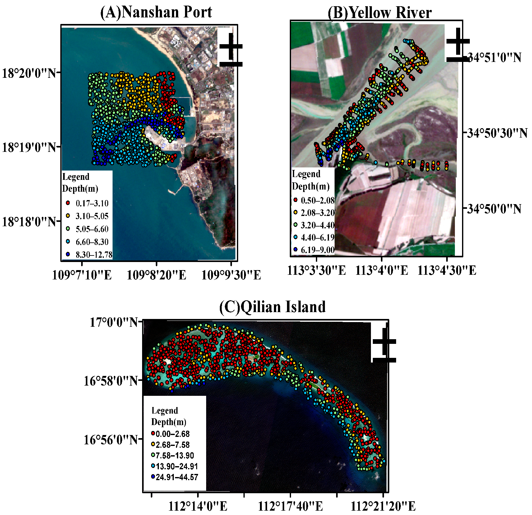
Figure 1. (A) represents the primary study area of Nanshan Port, while (B,C) denote the expanded study areas of the Yellow River and Qilian Islands.
Remotesensing 17 03712 g001
Figure 2. The workflow includes four main stages: The workflow includes four main stages: (A) Data Acquisition and Preprocessing; (B) Feature Engineering; (C) Stage 1 Base Learner Training; and (D) Stage 2 StackingMLP Meta-Learner Training. Each residual block consists of a linear layer, BatchNorm, GLU, and Dropout.
Remotesensing 17 03712 g002
Figure 3. IOPs Spatial Distribution.
Remotesensing 17 03712 g003
Figure 4. IOPs Pearson Correlation Plot. Band1 represents K d , Band2 represents a p h y ( 490 ) , and Band3 represents a d g ( 490 ) .
Remotesensing 17 03712 g004
Figure 5. Comprehensive performance analysis of base models. The plot compares four machine learning models (x-axis) across eight different feature combinations (colored lines). The results highlight the performance plateau and inconsistency when fusing physical features in a pixel-wise manner, with only marginal gains over the “Band Data” baseline.
Remotesensing 17 03712 g005
Figure 6. Validation scatter plots for the OptiFusionStack framework. Rows represent Nanshan Port (AC), Qilian Islands (DF), and the Yellow River (GI). Columns compare the baseline (Band Data only), best, and worst-performing feature combinations. The optimal configuration consistently outperforms the baseline in all environments.
Remotesensing 17 03712 g006
Figure 7. Heatmaps of depth-stratified error analysis. Each panel compares the baseline and best-performing models for a study area. Rows denote the model and depth interval (n = sample count). Columns represent RMSE and MRE metrics. The optimal OptiFusionStack model shows lower errors in nearly all depth bins across all sites.
Remotesensing 17 03712 g007
Figure 8. Visual comparison of spatial coherence. Top row (AC): Pixel-wise base models show significant spatial artifacts (red arrows). Bottom row (DF): The context-aware OptiFusionStack suppresses these artifacts but may smooth fine-scale features (blue arrows).
Remotesensing 17 03712 g008
Figure 9. Accuracy comparison against monolithic deep learning models. Herein, the gray dashed line represents the theoretically optimal fitting curve, while the red curve denotes the actual model fitting curve. Our OptiFusionStack framework (B) significantly outperforms a standard CNN (A), ResMLP (C), and Transformer (D), even when all models are trained on the exact same optimal input data.
Remotesensing 17 03712 g009
Figure 10. Decoupling of Features from Water Depth: The first four bands are satellite bands, with subsequent bands composed as indicated in the sub-figure captions.
Remotesensing 17 03712 g010
Figure 11. SHAP analysis of the top 20 features by importance.
Remotesensing 17 03712 g011
Table 1. The Physio-Spectral Feature Cube for Model Input.
Feature
Category
Feature NameSourceCenter Wavelength (nm)
Spectral
Features
R r s ( 490 ) Sentinel-2B Band 2–Blue492.1
Spectral
Features
R r s ( 560 ) Sentinel-2B Band 3–Green559.0
Spectral
Features
R r s ( 665 ) Sentinel-2B Band 4–Red664.9
Spectral
Features
R r s ( 833 ) Sentinel-2B Band 8–NIR832.8
Physical
Priors
a d g ( 490 ) QAA Calculation490
Physical
Priors
a p h ( 490 ) QAA Calculation490
Physical
Priors
K d ( 490 ) QAA Calculation490
Table 2. Detailed Input Feature Set for the Meta-Model (StackingMLP).
IndexFeature TypeDescriptionDimensions
1–4Point-wise
Predictive
The Out-of-Fold (OOF) depth predictions from the four base models: Random Forest, XGBoost, SVR, and CatBoost4
5–4 × iSpatial
Context (Spectral)
The mean, std, min, and max values of the original spectral bands within a 9 × 9 neighborhood window centered on the sample point.i × bands × 4stats = 4 × i
4 × i + 1 to 4 × i + 17Spatial
Context (Predictive)
The mean, std, min, and max values of the 4 base model prediction maps within a 9 × 9 neighborhood window centered on the sample point.4maps × 4stats = 16
Total
Dimensions
20 + 4 × i
Table 3. Sensitivity analysis of the neighborhood window size on the performance of the OptiFusionStack model, based on the K d + a d g ( 490 ) feature combination.
Neighborhood Window SizeR2RMSE (m)MAE (m)MRE
3 × 30.91360.61510.44490.0932
5 × 50.89330.68340.48500.0901
7 × 70.87800.73080.52140.0973
9 × 90.91670.58180.41130.1048
11 × 110.88020.72410.49680.0951
Table 4. Comparison of QAA-derived K d ( 490 ) with typical literature values.
Study AreaWater Type Derived   K d ( 490 ) Range (m−1)Typical
Literature Range (m−1)
Reference(s)
Qilian IslandsClear waters0.046–0.3350.05–0.15Hochberg (2003) [27]
Nanshan Portcoastal waters0.662–2.5350.03–10Qiu et al. (2013) [30]
Yellow Riverestuarine waters1.587–5.1520.17–59Sokoletsky & Shen (2014) [19]
Disclaimer/Publisher’s Note: The statements, opinions and data contained in all publications are solely those of the individual author(s) and contributor(s) and not of MDPI and/or the editor(s). MDPI and/or the editor(s) disclaim responsibility for any injury to people or property resulting from any ideas, methods, instructions or products referred to in the content.