Highlights
What are the main findings?
- Developed a standardized dataset for synthetic aperture radar block-type radio frequency interference, and simultaneously established a block-type interference mathematical model to provide theoretical support for interference data generation.
- Proposed a block-type interference suppression method based on image subspace, and completely decoupled interference suppression from imaging processes.
What are the implication of the main findings?
- By integrating laboratory-annotated data and Sentinel-1 satellite open-source measured data, the combined dataset can be directly used for training and validating deep learning models.
- Verified through three types of experiments—cross-dataset, same-distribution, and domain shift—this study summarizes the current research challenges and discusses potential future research directions.
Abstract
Synthetic aperture radar (SAR), as a high-resolution microwave remote sensing imaging technology, plays an indispensable role in both military and civilian applications. However, in complex electromagnetic countermeasure environments, radio frequency interference (RFI) severely degrades SAR imaging quality. SAR anti-interference, as a countermeasure method, has significantly practical values. Although deep learning-based anti-interference techniques have demonstrated notable advantages, two key issues remain unresolved: 1. Strong coupling between interference suppression and SAR imaging—most existing methods rely on raw echo data, leading to a complex processing pipeline and error accumulation. 2. Scarcity of labeled data—the lack of high-quality labeled data severely restricts model deployment. To address these challenges, this work constructs a standardized dataset and conducts comprehensive validation experiments based on this dataset. The main contributions are as follows: Firstly, this work establishes the mathematical model for block-type interference, laying a theoretical foundation for the subsequent construction of RFI-polluted data. Secondly, this work constructs a block-type interference dataset, which includes the labeled data constructed by our laboratory and open-source data from the Sentinel-1 satellites, providing reliable data support for deep learning. Thirdly, this work proposes an image subspace-based interference suppression method, which eliminates the dependence on raw echo data and significantly simplifies the processing pipeline. Finally, this work makes a fair comparison of the current works, summarizes the existing problems, and looks forward to possible future research directions.
1. Introduction
Synthetic aperture radar, as an advanced microwave imaging system, can provide all-weather and all-day high-resolution images [1,2], so it is widely applied in aerospace reconnaissance, aerial remote sensing, satellite marine observation, and agricultural remote sensing [3,4]. However, with the extensive deployment of various satellites for communication, navigation, radar, etc. in space, the electromagnetic environment has become increasingly complex, and radio frequency interference (RFI) has gradually evolved into one of the key challenges for SAR systems [5,6]. Moreover, most high-power ground-based radars can act as powerful interference sources, which makes SAR systems vulnerable [7,8,9]. The current academic community has also developed a variety of interference methods [10,11]. Among these, block-type interference is a widely existing interference pattern; for instance, even unintentional interference often generates block-type interference [12,13,14].
To address the appeal challenges, radar anti-interference technology has received extensive attention, and the existing researches can be summarized into three categories. 1. Radar anti-interference transmission technology: Its core is to perceive in real time multi-dimensional information such as the azimuth, power, modulation pattern, and forwarding rules of interference, and then to carry out the optimal design of radar transmission resources. Common methods include waveform design [15] and beam design [16,17,18]. Waveform design is to precisely adjust the waveform parameters to effectively counteract the interference signals, and beam design is to optimize the transmission beam to enhance the radar’s anti-interference ability in a complex electromagnetic environment. 2. Radar anti-interference reception technology: It mainly achieves anti-interference by designing receiving filters in multiple dimensions such as the spatial domain, time domain, frequency domain, and polarization domain. During the accumulation of target echo energy, the energy of interference signals is simultaneously suppressed. The relevant technologies cover anti-interference receiving beamforming [19,20,21], time-domain filtering [22,23], Doppler-domain filtering [24], polarization-domain filtering [25], and joint multi-domain filtering [26], etc. 3. Radar anti-interference processing technology: This technology focuses on amplifying the differences between interference and targets across multiple domains (such as spatiotemporal, frequency, polarization, etc.), and then effectively separates the interference from the targets [6,27].
According to published academic literatures, most current radar anti-interference methods in system level are mainly applicable to active phased array radars rather than synthetic aperture radars, because SAR is mainly used for imaging and does not possess the ability to perceive interference. It is worth noting that radar anti-interference processing technology shows good adaptability in the application of synthetic aperture radars, as it has no specific constraints on the radar systems. Among them, as an efficient radar anti-interference processing technology, the interference suppression technology can be roughly divided into non-parametric methods, parametric methods, and semi-parametric methods.
Non-parametric methods include notch filters [28,29,30], adaptive filters [31,32,33], and subspace projection filters [34,35,36,37]. Non-parametric methods are relatively simple, while they require significant characteristic differences between the interference signals and the radar signals. When the characteristic differences are not obvious, their performance is insufficient. Parametric methods first model the interference signals and then subtract the fitted interference signals from mixed signals [38,39,40]. Mostly, their performance is not clear, especially for some complex scenarios. Unlike parametric methods, semi-parametric methods do not directly model the interference signals, but mainly use sparse constraints or low-rank constraints to iteratively separate the interference signals from mixed signals. These methods can filter out interference signals and also protect target signals, so their performance is better. Many iterative models have been proposed, including sparse models [41,42,43], low-rank models [44,45,46,47], and joint sparse low-rank models [42,48,49,50,51]. Although semi-parametric methods perform well, they are more time-consuming.
At present, some studies have proven that deep learning methods are feasible, but most of these methods are variants of non-parametric methods [52,53,54]. Furthermore, previous work introduced a deep learning method into SAR interference suppression for the first time [55]. Previous work injected the sparsity of interference and the low rank of signals into the loss function to improve its performance, and finally its performance exceeds the semi-parametric methods such as robust principal component analysis [56]. Previous work proposed a joint image segmentation and image inpainting network, which first uses a segmentation network to separate the variable interference components, and then uses an inpainting network for image restoration [14]. Previous work proposed a regularized optimization feature decomposition network, which can greatly reduce the difficulty of data fitting by optimizing the regularization term [13]. Previous work proposed a two-stage self-supervised learning method, with the first stage being a segmentation network and the second stage being an image restoration network [57].
Despite the growing research interest in deep learning methodologies, their progress in this specific application remains relatively limited, primarily due to the following reasons: 1. Strong coupling between interference suppression and SAR imaging. Currently, the vast majority of interference suppression methods focus on SAR echoes. After interference suppression, post-processing to the raw echoes is still required to obtain SAR images. This tight integration of interference suppression and SAR imaging not only increases the complexity of the overall processing flow but also risks error accumulation. 2. The problem of inadequate data, especially the scarcity of precisely labeled samples, makes model training and quantitative evaluation challenging, ultimately hindering the application of deep learning approaches in interference suppression. To address the above challenges, first of all, this work publicly releases a dataset of block-type radio frequency interference based on Sentinel-1 satellites and elaborates in detail the mathematical principles of the block-type radio frequency interference. Secondly, comprehensive experiments are carefully carried out based on the image subspace. The experimental results show that the network trained on this dataset exhibits excellent generalization ability and can be efficiently applied to the measured interference data of Sentinel-1 satellites. Therefore, the published dataset has important practical value and is expected to promote the development of this field. The contributions are as follows:
- We have publicly released a SAR block-type radio frequency interference dataset, which includes not only precisely annotated data but also unlabeled measurement data from Sentine-1 satellites. To the best of our extensive knowledge, this is the first block-type radio frequency interference dataset, filling a critical gap in data resources.
- We have established a mathematical model of block-type interference, laying a theoretical foundation for the subsequent construction of the dataset. Additionally, it also facilitates others to build their own datasets through this method.
- We propose an interference suppression method based on the image subspace, which doesn’t require the transformation between SAR echoes and SAR images. This characteristic enables the method to break away from the dependence on raw echo data, greatly simplifying the interference suppression pipeline.
- We make a fair comparison of the current work, summarize the existing problems in the current research, and look forward to possible future research directions.
The subsequent arrangement is as follows: Section 2 elaborates in detail the construction method of the interference dataset and the mathematical principles involved behind it, providing a solid theoretical basis for the generation of the dataset. Section 3 provides a comprehensive introduction to the constructed dataset, including the composition, characteristics, and application scenarios. Section 4 clarifies the interference suppression process and specific implementation details. Section 5 makes a fair comparison of the current works, and summarizes the existing problems in the current researches. Section 6 summarizes the full text, and points out the potential research directions for the future.
2. The Model of Block-Type Radio Frequency Interference in Strip-Mode
In the SAR imaging, the complex electromagnetic environment has become a critical factor limiting SAR image quality. Among these, block-type RFI is a widely existing interference pattern. As shown in Figure 1a, multiple interference signals with distinct frequency, amplitude, and phase characteristics coexist simultaneously throughout the radar pulse duration and exhibit specific distribution patterns. These interference signals will introduce complex distortions to the radar echoes. When the interference is superimposed on the radar echo signals, the result is depicted in Figure 1, where a complete overlap between the radar and interference signals is clearly observed, with signals of varying frequencies, amplitudes, and phases intricately intertwined. In practical SAR imaging, specialized focusing algorithms are employed to extract target information from the complex echoes and high-quality SAR images can be obtained. However, due to the complete aliasing between radar and interference signals, the focusing process inevitably enhances both the desired signals and the interference, leading to a decline in image quality. Therefore, a systematic investigation into the mechanism of radio frequency interference on SAR images is of paramount importance. By analyzing the characteristics of interference signals, and their propagation and transformation, we can comprehensively understand how RFI deteriorates SAR images. This research will provide a robust theoretical foundation for anti-interference techniques and facilitate the development of more effective suppression methodologies. Certainly, there are numerous interference patterns, while this study only focuses on block-like radio frequency interference in strip-mode SAR, thus it has some limitations shown as follows: (1) The modulation mode of the interference signal remains unchanged throughout the entire interference period. (2) The SAR operates in the strip-mode. (3) The tuning rates of the interference signal and the radar signal are different.
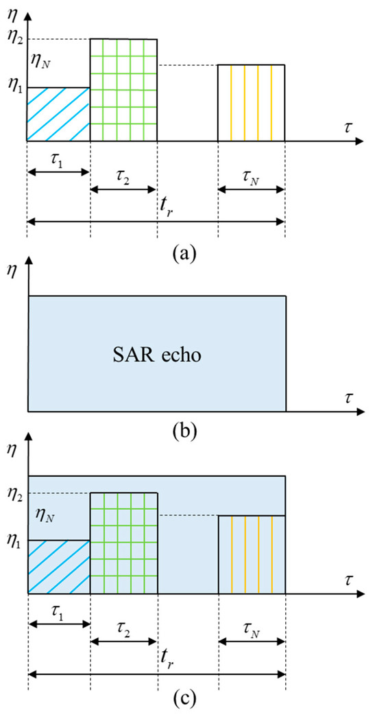
Figure 1.
The process of the radar being jammed by interference signals. (a) The interference echo. (b) SAR echo. (c) RFI-polluted SAR echo. Among them, represents the range time, and represents the azimuth time. represents the radar pulse duration, represents the range pulse duration of the first interference, represents the range pulse duration of the second interference, and represents the range pulse duration of the N-th interference. represents the azimuth pulse duration of the interference.
The common RFI can be categorized into three types: narrowband interference, chirp-modulation wideband interference, and sinusoidal-modulation wideband interference, and this work has established mathematical models for the above three RFI signals. Narrowband interference is composed of a series of single-frequency signals and can be represented as follows:
wherein, , and are sequentially represented as the carrier frequency, the amplitude and the frequency offset, and represents the number of the interference signals. The chirp-modulation wideband interference can be represented as follows:
wherein, and are sequentially represented as the amplitude and the chirp rate. The sinusoidal-modulation wideband interference can be represented as follows:
wherein, , and are sequentially represented as the amplitude, the modulation coefficient and the modulation frequency. According to the first Bessel function, the sinusoidal-modulation wideband interference can also be expressed as follows:
wherein, . According to (4), it can be seen that the sinusoidal-modulation wideband interference is composed of a series of narrowband interferences. So, the above three interference signals can be uniformly expressed as follows:
wherein, represents the amplitude, and represents RFI chirp rate. It can be seen that when is relatively large, this expression can be approximated as a wideband interference, and when is relatively small, it degenerates into a narrowband interference.
In most scenarios, multiple interference signals will coexist within a single radar pulse duration, as depicted in Figure 1. Crucially, Equation (5) demonstrates that these interference signals obey the principle of linear superposition. This fundamental property indicates that even when the actual interference consists of multiple components, conducting an in-depth analysis of a single representative interference source can precisely and effectively elucidate the core influence mechanisms of block-type interference on SAR systems. Taking a single interference source as an exemplar case, the imaging geometry is illustrated in Figure 2, where the radar platform moves with a velocity of v along the trajectory from point B to point A. During synthetic aperture formation, the radar system regularly samples the target and jammer and the sampling points are shown as dots in Figure 2. The vertical distance between the target and the radar is denoted as , the vertical distance between the jammer and the radar is denoted as , the instantaneous slant range between the target and the radar is denoted as , the instantaneous slant range between the jammer and the radar is denoted as , and represents the azimuth time.
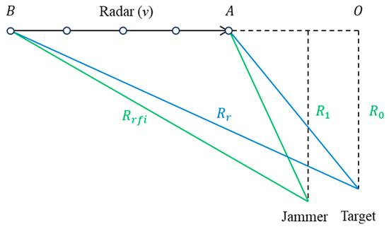
Figure 2.
The geometric model of strip-mode SAR. The radar moves from point B to point A at a speed of and samples the target and the jammer regularly. Among them, represents the slant range between the target and the radar, represents the slant range between the jammer and the radar. represents the vertical distance between the radar and the target, and represents the vertical distance between the radar and the interference.
At this time, the interference signal can be expressed as follows:
wherein, represents the range time, denotes a rectangular pulse signal, indicates the interference pulse duration, represents the carrier frequency, and denotes the interference chirp rate.
2.1. Range Compression
As shown in Figure 2, the received 2-D interference signal can be represented as follows:
wherein, , , and denotes a single synthetic aperture duration. The de-chirp range compression can be expressed as follows:
wherein, the reference signal can be expressed as follows:
The core of de-chirp processing lies in achieving signal demodulation through the mixing operation of the echo signal and the reference signal, and the de-chirp signal can be represented as follows:
According to the principle of stationary phase, the de-chirp range compression of the interference can be expressed as follows:
wherein, .
2.2. Range Cell Migration Correction
Usually, stripe-mode SAR conforms to far-field approximation, therefore, the instantaneous slant range between the interference and the radar can be expressed as follows:
Combining (11) and (12), the interference signal is shown as follows:
Through azimuth Fourier transformation, the interference signal can be expressed as follows:
wherein, represents the azimuth frequency, denotes the azimuth chirp rate of the interference signal, and denotes the range cell migration component. After correcting range cell migration component, the interference signal is given by:
2.3. Azimuth Compression
The azimuth matched filter is given by:
wherein, represents the azimuth chirp rate of the reference signal. According to principle of stationary phase, by azimuth compression, the interference signal can be expressed as follows:
wherein, .
According to (17), it can be seen that the interference signal appears as a block-type signal, and usually, the interference regions typically exhibit extensive coverage and high intensity, severely distorting target areas in the image and consequently significantly degrading SAR image quality. So, radar anti-jamming technology has become a prominent research focus in the field of electronic information. By modeling block-type interference under various parameters and scenarios, and superimposing these onto SAR echo signals, a substantial volume of labeled samples can be generated. These comprehensive samples provide abundant data resources for subsequent research on radar anti-jamming, as well as for model training and testing, thereby significantly enhancing radar’s anti-jamming capabilities in complex electromagnetic environments.
3. Dataset
During the imaging process of Sentinel-1 satellites, they often suffer from intentional or unintentional radio frequency interference from ground or space-based sources, which may be severe enough to blind SAR satellites, significantly impairing their data acquisition capabilities. To effectively address this challenge, many researchers have proposed numerous methods. However, for non-parametric, parametric or semi-parametric methods, it remains difficult to achieve an ideal balance between performance and efficiency. Deep learning, as an emerging technological paradigm, holds promise for resolving these issues. In the current radar anti-jamming, the scarcity of labeled samples remains a critical challenge. On one hand, the lack of training data makes the application of existing deep learning methods in radar anti-jamming scenarios particularly challenging. On the other hand, without sufficiently diverse and representative test data, it is impossible to comprehensively and accurately evaluate the model’s performance under different interference conditions, making it difficult to identify their bottlenecks. Therefore, preparing a comprehensive dataset has become one of the primary challenges that urgently need to be addressed in the field of radar anti-jamming. So, this work releases a dataset of block-type interference, which includes the data constructed by our laboratory and open-source data from the Sentinel-1 satellites.
All dataset originates from European Sentinel-1 satellites. Sentinel-1 is a constellation system consisting of two identical SAR satellites. Among them, Sentinel-1A was successfully launched on 3 April 2014, while Sentinel-1B entered its designated orbit on 25 April 2016. These two satellites are positioned 180 degrees apart in the same orbital plane, which enables optimal global coverage and efficient data transmission. With this constellation system, a global imaging task can be completed every six days. Its applications are wide-ranging, covering key areas such as ocean remote sensing, marine environment surveillance, ship detection for maritime security, monitoring of tectonic plate movements for risk assessment, mapping for forest, water, and soil management, as well as supporting humanitarian aid and crisis response through cartography. The radar parameters are shown in Table 1. The radar operates in the C-band with a frequency of 5.4 GHz, and the imaging mode is strip-mode. The pulse duration ranges from 5μs to 100μs, with a radar bandwidth of less than 100 MHz. The range resolution reaches 5.90 m, while the azimuth resolution reaches 19.90 m. The polarization modes include either HH+HV or VV+VH.

Table 1.
Parameters of strip-mode Sentinel-1 satellites.
3.1. The Data Constructed by Our Laboratory
Based on the imaging model elaborated in Section 2, we established a labeled dataset. This dataset comprises a total of 640 image slices, each with dimensions of 512 × 1500 pixels and containing 1500 test samples. Each image slice is stored separately as a MATLAB2022 formatted file (.mat), which contains two sets of complex image data (i.e., the RFI-polluted image and the RFI-free image), as well as key information such as interference related parameters. The image slices incorporate four distinct signal-to-interference ratios (SIRs), eight different interference patterns with varying parameters, and four representative imaging scenarios. When the signal-to-interference ratio is equal to −20 dB, the example diagrams of different imaging scenarios are shown in Figure 3, the horizontal axis represents the azimuth direction, the vertical axis represents the range direction, and the scenarios are successively maritime zone, harbor area, urban region, and mountainous terrain. As shown in Figure 3, the targets covered by interference are completely obscured, and it is difficult to identify any contours and details of the interfered targets, which fully demonstrates that the interference has caused serious damage to SAR images.
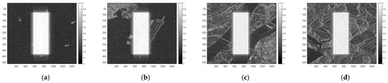
Figure 3.
RFI-polluted images under different scenarios in constructed data, among them, the white part is the RFI-polluted area. (a) Maritime zone. (b) Harbor area. (c) Urban region. (d) Mountainous terrain.
The interference parameters are shown in Table 2, and it covers four signal-to-interference ratios, namely −30 dB, −20 dB, −10 dB, and 0 dB. As described in [56], the signal-to -interference ratio (SIR) here is defined as the ratio of the average power of the target signal in the interfered area to the average power of the interfering signal. The imaging results under four different signal-to-interference ratios are shown in Figure 4, the horizontal axis represents the azimuth direction, and the vertical axis represents the range direction. It can be clearly observed that the effects of interference vary significantly under different signal-to-interference ratios. When the signal-to-interference ratio is equal to 0 dB, the contours of most targets are relatively clear, and the general shapes and features of the targets can still be identified. When the signal-to-interference ratio drops to −10 dB, a significant change occurs. At this time, the contours of most targets become blurred, a large amount of detailed information is lost, and only a little isolated strong scattering points remain. When the signal-to-interference ratio further decreases to −20 dB or −30 dB, almost all targets are covered by interference, and it is difficult to find any trace of the targets in the image. Additionally, in practical radar detection, radar signals are typically target-reflected waves, while radio frequency interference signals are mostly direct waves. Direct waves incur less loss during propagation, whereas target-reflected waves experience significant attenuation. As a result, the interference power usually significantly exceeds the target-reflected power. This physical reality means that in most practical scenarios, the signal-to-interference ratio remains below −20 dB. Consequently, in the interfered area, targets are completely obscured by interference. This phenomenon clearly demonstrates that such interference can significantly degrade the quality of radar images.
Table 2.
Interference parameters.
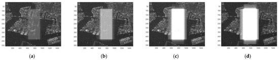
Figure 4.
RFI-polluted images under different signal-to-interference ratios in constructed data, among them, the white part is the RFI-polluted area. (a) 0 dB. (b) −10 dB. (c) −20 dB. (d) −30 dB.
3.2. Open-Source Data by Sentinel-1 Satellites
The released dataset further includes the open-source data consisting of 30 image slices, each with dimensions of 512 × 1500 pixels and containing 1500 test samples. Similar to the above dataset, we have meticulously categorized the imaging scenarios into four representative types: maritime zone, harbor area, urban region, and mountainous terrain. The RFI-polluted images of different scenarios are shown in Figure 5, depicting a sea area, urban area, port, and mountainous region in sequence; the horizontal axis represents the azimuth direction, and the vertical axis represents the range direction. From these four diagrams, it is visually evident that the interference intensity is extremely high, with signal-to-interference ratios below −20 dB, causing targets to be completely submerged in noise. Specifically, the first and second diagrams reveal an extremely complex interference scenario: there exist both high-intensity interference regions characterized by large-area and dense noise coverage and low-intensity interference regions with relatively sparse distributions. The third and fourth diagrams clearly show the presence of at least two types of combined interferences, where different interference types overlap, further increasing interference complexity. Figure 6 presents images under partial low-interference conditions with a signal-to-interference ratio close to 0 dB, the horizontal axis represents the azimuth direction, and the vertical axis represents the range direction. Although the interference does not completely drown out the targets, the quality of the interfered SAR images has severely degraded: target edges in the images are blurred, and a large amount of detailed information is lost. The above results demonstrate that the interference has an extremely wide coverage and causes severe adverse effects, rendering SAR images unusable.
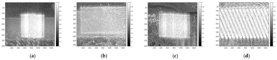
Figure 5.
RFI-polluted data under strong interference in open-source data, among them, the white part is the RFI-polluted area. (a) Maritime zone. (b) Harbor area. (c) Urban region. (d) Mountainous terrain.
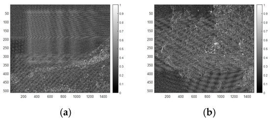
Figure 6.
RFI-polluted data under weak interference in open-source data, among them, the white chaotic part is the RFI-polluted area. (a) Maritime zone. (b) Urban region.
4. Interference Suppression
Under the current research paradigm, most methods predominantly focus on the SAR echo domain. Specifically, these approaches first perform interference suppression at the SAR echo stage, and then apply imaging algorithms to convert SAR echoes into SAR images. However, this operational mode results in a tight coupling between SAR interference suppression and SAR imaging. Despite the availability of open-source datasets, the interference suppression remains highly challenging due to the general lack of SAR imaging knowledge. This highlights that developing an interference suppression method based on the image subspace has become a core challenge in this field. To effectively address this issue, this work proposes an image subspace-based interference suppression method tailored for the block-type radio frequency interference. A notable advantage of this method is its exclusive reliance on SAR images, eliminating the switching between SAR echoes and SAR images. As a result, it successfully decouples block-type interference suppression from complex and cumbersome imaging algorithms. This feature provides significant convenience to subsequent researchers, allowing them to focus entirely on in-depth studies of interference suppression without expending excessive effort on the interconnections with complex imaging algorithms. The pipeline is shown as Algorithm 1.
| Algorithm 1. Block-Type Interference Suppression in Image Subspace |
| Input: RFI-polluted image (SMXN), azimuth point (M), range point (N) Output: RFI-free image (S*) for i = 1:M X = S(i,:); // Step I X = stft(X); // Step II X = H(X); // Step III X = istft(X); // Step IV S*(i,:) = X; // Step V end |
4.1. Interference Suppression Based on Image Subspace
Step I. De-compose 2-D complex images into 1-D range signals. According to (17), when we decompose the block-type interference into a series of one-dimensional (1-D) range signals, the 1-D range signal of block-type interference can be expressed as follows:
wherein, in the k-th azimuth pulse, the amplitude of (17) can be expressed as follows:
Step II. Short-time Fourier transform. Equation (18) indicates that the interference signal is a wideband signal. Suppressing wideband interference signals is more challenging in a single time or frequency domain, but relatively simpler in the joint time-frequency domain. Thus, we can transform the above signals into the joint time-frequency domain. Among them, represents the window-function, and the time-frequency transform can be expressed as follows:
Preliminary experiments have shown that the influence of window function type is not significant, so the commonly used Hamming window is adopted. The window length is typically in the range of 1/8 to 1/4 of the data length L (where L denotes the number of sampling points), and L/8 is selected in this study.
Step III. Suppress interference by deep learning networks. We utilize a deep learning network to map RFI-polluted time-frequency signals to RFI-free time-frequency signals. Here, the input to the network is the RFI-polluted time-frequency signal (), the output is the RFI-free time-frequency signal (), and the network’s matrix function is defined as . This mapping process can be expressed as follows:
Step IV. Inverse short time Fourier transform. Step IV serves as the inverse operation of Step II, aiming to transform the time-frequency signals back to the original domain.
Step V. Transform multiple sets of 1-D signals into 2-D complex images. Step V acts as the inverse operation of Step I, designed to convert the 1-D range signals back into 2-D complex images. Following this processing, the RFI-free SAR images can be obtained.
4.2. Evaluation Metrics
According to [14], this work also employs three evaluation metrics: peak signal-to-noise ratio (PSNR), structural similarity (SSIM), and mean-entropy (ME). In the image quality assessment framework, PSNR and SSIM calculations rely heavily on paired labeled data, enabling precise quantitative evaluations of structural and pixel-wise consistency. By contrast, ME is a self-evaluation metric that only provides a coarse assessment and lacks the ability to accurately evaluate fine details such as structure and texture. For our constructed data, since the corresponding label data exists, PSNR and SSIM can be employed to conduct quantitative comparisons of results from different networks, which helps identify the limitations of each network. For open-source data by Sentinel-1 satellites, due to the shortage of labeled data, we can only use ME to conduct a preliminary assessment of the output results. This metric is capable of quantifying the discrepancies between network outputs and interfered images, yet it remains insufficient to discern nuanced performance disparities across different networks.
PSNR represents the noise level, and the larger PSNR, the better performance. PSNR is presented as follows:
wherein, denotes the output of the network, and denotes the ground-truth, denotes the root-mean-square, and H and W represent the pixel numbers. SSIM can be expressed as follows:
wherein, denotes the mean value, denotes the variance or the covariance. A higher structural similarity indicates better performance. ME is defined as follows:
wherein, denotes the entropy, denotes the mean value. A smaller entropy indicates a clearer image, and a smaller mean value indicates lower interference, so a smaller ME indicates better performance.
4.3. Implementation Details
To establish a rigorous and reproducible experimental framework, all model training and evaluations were executed on a standardized hardware platform comprising a 20-core Intel Core i7-14700 K processor (2.50 GHz base frequency) and NVIDIA GeForce RTX 3090 GPU with 24 GB dedicated memory. Utilizing the curated dataset, we systematically trained and evaluated the distinct state-of-the-art detection architectures under identical configurations. For standardized comparison, each model underwent 100-epoch training cycles with a uniformly applied batch size of 4, ensuring consistent computational throughput and memory utilization patterns across all experimental iterations. The initial learning rate is set to 0.0002, and the AdamW optimizer is adopted.
5. Experiment
To comprehensively evaluate the validity of the dataset published in this work, we carefully designed and conducted three groups of experiments. In the first group, the data constructed by our laboratory was used as training data, and the open-source data from Sentinel-1 served as testing data. This experimental setup aims to examine whether a network trained on our constructed data can effectively generalize to real-world interference scenarios. If the network performs well on real RFI-polluted Sentinel-1 data, it can be reasonably inferred that our modeling of block-type RFI is accurate. In the second group, both the training and testing data are derived from our constructed data and adhere to the same data distribution. This experiment focuses on investigating the prediction ability of models within the same data distribution, which is conducive to thoroughly uncovering the performance differences among different models. In the third group, although both testing and training data originate from our constructed data, they do not adhere to the principle of identical data distribution—i.e., significant differences exist in interference parameters between training and testing data. Through this experiment, we can explore how the model’s performance changes when facing inconsistent interference parameters between training and test data. The above studies can identify the current shortcomings and provide directions for subsequent research.
We carefully select the representative models to conduct comprehensive and in-depth validation experiments. The models include DNCNN [55], PISNet [56], UNet [57], and FDNet [13]. Among them, DNCNN, PISNet, and UNet belong to the CNN-based network model family. Leveraging the unique advantages of convolutional neural networks in feature extraction, they have demonstrated excellent performance in numerous past studies and practical application scenarios. FDNet is part of the Transformer-based network model family, showcasing outstanding capabilities in capturing long-range dependency relationships. During the experiment, we keenly observed a crucial issue in PISNet: the final sigmoid layer caused significant convergence difficulties during the training process. After in-depth analysis, this phenomenon may stem from the inherent characteristics of the sigmoid function, which can easily lead to gradient vanishing or gradient explosion, thus impeding the update of network parameters. Moreover, from a physical perspective, the additional non-linear processing added in the last layer of PISNet lacks a clear and reasonable explanation. Based on these two considerations, we decisively removed the final sigmoid layer in PISNet. Additionally, it is worth noting that in the interference suppression, high-power and variable interference components pose significant challenges to the networks. This work employs the data regularization method proposed in [13] during the data preprocessing stage, and this method can counteract the aforementioned impacts to a certain extent. The expression is shown in Equation (26), where Y denotes the label, X denotes RFI-polluted image, and Xmax represents the maximum value of X. By providing a higher-quality data for subsequent training, it significantly enhances the network’s performance in complex interference environments.
5.1. Experiment Under the Open-Source Data from Sentinel-1
To fully verify the reliability of our dataset, this study first conducted validation experiments based on the open-source data from Sentinel-1. In this experiment, the training data was from our constructed dataset, while the testing data was from Sentinel-1 satellites. It is worth noting that the patterns and power of the actual interference are unknown, so the constructed data must closely resemble real-world interference scenarios to ensure that the training network is effective. Time-frequency spectrums are shown in Figure 7, the horizontal axis represents the time unit, and the vertical axis represents the frequency unit. SAR images are shown in Figure 8, the horizontal axis represents the azimuth direction, and the vertical axis represents the range direction. As clearly seen from Figure 7, FDNet demonstrated the most outstanding performance, which justifies that Transformer-based network has superior capabilities in feature extraction. Figure 8 clearly shows that the relative motion in the range direction between the interference source and the radar leads to significant slant-range shifts in blocky interference. Fortunately, all networks effectively eliminate the above interference. Additionally, in the transition zone between non-interference and interference regions, the target structure transitions naturally. Based on these results, we can reasonably infer and conclude that: networks trained by our constructed dataset possess excellent generalization capabilities and can be effectively applied to practical interfered datasets. This discovery strongly confirms that our modeling of interference is correct. The dataset we constructed is highly consistent with the interference dataset sourced from the open data of Sentinel-1 satellites, and the dataset we constructed can serve as a substitute for Sentinel-1 data. The examination of Table 3 reveals that there are almost no differences among these three methods in ME, so relying solely on the self-assessment method is insufficient to fully uncover the performance limitations in practical applications. Therefore, for subsequent research, constructing matched label samples has become a key step to deeply explore and identify such limitations, and it will provide important guidance for the optimization and improvement of the network.
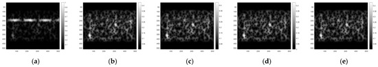
Figure 7.
Time-frequency spectrum of open-source data from Sentinel-1. (a) RFI-polluted Time-frequency spectrum. (b) Time-frequency spectrum by DNCNN. (c) Time-frequency spectrum by PISNet. (d) Time-frequency spectrum by UNet. (e) Time-frequency spectrum by FDNet.
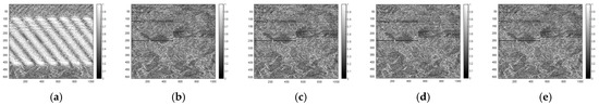
Figure 8.
SAR images of open-source data from Sentinel-1, among them, the white part is the RFI-polluted area. (a) RFI-polluted SAR image. (b) SAR image by DNCNN. (c) SAR image by PISNet. (d) SAR image by UNet. (e) SAR image by FDNet.
Table 3.
Mean-entropy Under the Open-source Data from Sentinel-1.
5.2. Experiment Under the Same Data Distribution
In the experiment under the same data distribution, we carefully select the dataset with a signal-to-interference ratio (SIR) of −20 dB as the training data, while the testing data included different signal-to-interference ratios: 0 dB, −10 dB, −20 dB, and −30 dB. The results under these conditions are presented in Figure 9. We can clearly observe that as the SIR decreases, the PSNR and SSIM of the RFI-polluted images shows a gradual downward trend. Fortunately, all four methods significantly improve the PSNR and SSIM. When the SIR is greater than or equal to −20 dB, the four methods can effectively mitigate the interference and achieve satisfactory results. However, when the SIR drops to −30 dB, the performance of all methods declines, which clearly indicates that high-power interference poses significant challenges to networks, making it difficult to accurately reconstruct clean data. Among the four methods, FDNet performs better and is more robust to the noise power. Under the four different SIR conditions, FDNet maintains a PSNR above 30 dB and an SSIM greater than 90%. In contrast, PISNet and DNCNN are more significantly affected by different SIRs—their performance declines sharply as the SIR decreases. Furthermore, it is precisely because the constructed data includes ground truth that we can conduct a more detailed and comprehensive evaluation of the images. This meticulous evaluation allows us to keenly identify the shortcomings of the current networks, which in turn provides a clear direction for further model optimization. By adjusting the network architecture, parameter settings, or training strategies, researchers can gradually improve model performance and significantly enhance image quality.
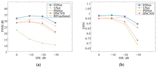
Figure 9.
Experimental results of different signal-to-interference ratios under the same data distribution. (a) PSNR. (b) SSIM.
We further present the experimental results when the SIR is equal to −20 dB. The time-frequency spectrums are shown in Figure 10, the horizontal axis represents the time unit, and the vertical axis represents the frequency unit. SAR images are shown in Figure 11, the horizontal axis represents the azimuth direction, and the vertical axis represents the range direction. As clearly observed in Figure 10, the time-frequency spectrum suffers severe interference contamination, with originally distinct signal characteristics being completely obscured by substantial chaotic interference. Compared with the ground truth, most of methods still exhibit minor residual noise, while FDNet demonstrates superior performance. A close examination of Figure 10 reveals that the interference signals are extensively distributed throughout the entire spatial domain. Under such conditions, FDNet demonstrates superior performance by leveraging its unique global feature extraction capability. As can be seen from Figure 11, when the SIR is equal to −20 dB, the target is almost completely obscured by the interference, making it difficult to directly identify the contours and details of the targets. This fully highlights the powerful destructive effect of high-intensity interference on SAR images. After training the network with the publicly available dataset, it is exciting to note that the four methods exhibit excellent interference suppression capabilities and can eliminate the vast majority of interference. More importantly, the detailed structures of the SAR images are fully reconstructed. The above indicates that when the training data and the testing data have the same distribution, the block-type interference can be effectively eliminated.
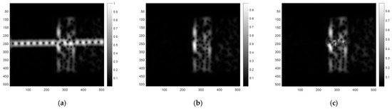
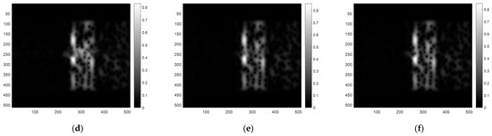
Figure 10.
Time-frequency spectrums under the same data distribution with a signal-to-interference ratio of −20 dB. (a) RFI-polluted. (b) Ground Truth. (c) DNCNN. (d) PISNet. (e) UNet. (f) FDNet.
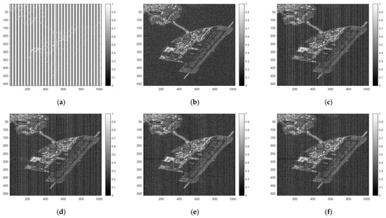
Figure 11.
SAR images under the same data distribution with a signal-to-interference ratio of −20 dB, among them, the white part is the RFI-polluted area. (a) RFI-polluted. (b) Ground Truth. (c) DNCNN. (d) PISNet. (e) UNet. (f) FDNet.
5.3. Experiment Under the Domain Shift Condition
Whether it is intentional interference or unintentional interference, the modulation modes of interference signals are likely to differ. While interferences with different modulation modes show minor differences in the image domain, they exhibit considerable distribution shifts in the signal space, which may lead to the above methods failure. When significant distribution shifts occur between training and test data, the test results for different signal-to-interference ratios are shown in Figure 12. Evidently, compared with the original interfered data, the image quality improves under four conditions. When the signal-to-interference ratio is equal to 0 dB or −10 dB, the PSNR exceeds 30 dB, and the SSIM approaches or exceeds 90%. The above indicates that the network remains effective in a weakly interfered environment, and the image quality is relatively high after interference suppression. However, when the signal-to-interference ratio is below −20 dB, the PSNR and SSIM deteriorate sharply, and there are no significant differences between different networks. Under this condition, the PSNR drops below 25 dB. These experimental results strongly indicate that when a significant distribution shift occurs between training and testing data, model performance degrades, so data distribution shift has become one of the key challenges in SAR interference suppression. Additionally, experimental results under −20 dB interference condition are shown in Figure 13, the horizontal axis represents the azimuth direction, and the vertical axis represents the range direction. It can be observed that although most of the interference has been removed, residual interference components remain in the SAR images, and targets exhibit significant distortion. These observations indicate that data distribution shift has emerged as a critical challenge, exerting a non-negligible negative impact on radar signal processing and interference suppression. Addressing data distribution shift and enhancing model generalization will therefore become one of the main focuses for future research.
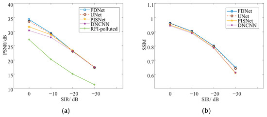
Figure 12.
Experimental results of different signal-to-interference ratios under the domain shift condition. (a) PSNR. (b) SSIM.
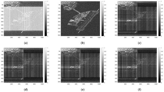
Figure 13.
SAR images under the domain shift condition with a signal-to-interference ratio of −20 dB, among them, the white part is the RFI-polluted area. (a) RFI-polluted. (b) Ground Truth. (c) DNCNN. (d) PISNet. (e) UNet. (f) FDNet.
5.4. Experiment Under Different Domains
The experimental results of the image subspace and echo domain are shown in Figure 14. Compared with the echo domain, the proposed image subspace method exhibits a slight advantage in comprehensive performance, with the most significant improvement achieved under the condition of −30 dB signal-to-interference ratio: the PSNR is improved by 0.96 dB, and the SSIM is improved by 0.06. In addition, the proposed image subspace method can decouple the interference suppression process from the imaging workflow, which significantly simplifies the overall processing pipeline and enhances the engineering practicality of the method.
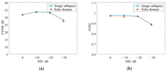
Figure 14.
Experimental results of different signal-to-interference ratios under different domains. (a) PSNR. (b) SSIM.
6. Conclusions and Discussion
As a high-resolution imaging radar, SAR has demonstrated extensive and significant application value across various fields. However, the quality of SAR images can severely degrade when subjected to interference during the imaging process, significantly limiting their actual effectiveness. Among various interference patterns, the block-type interference is a prevalent type. While numerous methods have been proposed to address this issue, classical approaches struggle to achieve an ideal balance between performance and efficiency. The rise of deep learning technology has provided new opportunities to resolve this dilemma. Nevertheless, the lack of training and testing data—particularly the severe shortage of labeled data—has greatly hindered effective training and precise evaluation of deep learning models, and emerges as a critical bottleneck. To address these challenges, this work makes the following contributions: First, this work establishes the mathematical formulation of block-type interference, laying a robust theoretical foundation for constructing RFI-polluted data. Second, a publicly accessible SAR block-type interference dataset is released, which integrates both the labeled data form our laboratory and field-measured data form Sentinel-1 satellites. Third, an image subspace-based anti-interference method is proposed. This approach successfully decouples SAR interference suppression from SAR imaging. Fourth, a comprehensive and rigorous validation is conducted on the published dataset using the most advanced methods in the field of interference suppression. Furthermore, from an experimental perspective, we have identified certain current limitations and proposed potential research directions. 1. The scarcity of labeled samples remains a critical bottleneck. Due to the high complexity and specificity of radar countermeasure scenarios, there is a severe shortage of matched labeled samples, which causes significant difficulties in model training. So, exploring deep learning models based on weakly supervised or unsupervised learning has become one of the important research directions. 2. Data distribution shift is another critical challenge hindering the transition of deep learning models from theory to practical application. When significant distribution shifts exist between training and testing data, their performance deteriorates sharply. Therefore, improving the generalization capability of models and ensuring their effectiveness across scenarios with different data distributions has become another formidable problem.
Author Contributions
Conceptualization, F.F.; methodology, F.F. and S.Q. software, F.F.; validation, D.D. formal analysis, Y.T.; investigation, D.D. resources, Y.T.; data curation, D.D.; writing–original draft preparation, F.F.; writing–review and editing, S.Q. and Y.T.; visualization, Y.T.; supervision, S.X. and Y.T.; project administration, D.D.; funding acquisition, S.Q., Y.T. and F.F. All authors have read and agreed to the published version of the manuscript.
Funding
This work was supported by the National Natural Science Foundation of China under Grant 62471471, 62001489, and the China Postdoctoral Science Foundation under Grant 2024M754307.
Data Availability Statement
Data available in a publicly accessible repository (https://github.com/fangfuping/SAR-RFI-DATASET (accessed on 30 June 2025)).
Acknowledgments
Thanks to the European Sentinel-1 satellites for their data supports.
Conflicts of Interest
The authors declare no conflicts of interest.
References
- Cruz, H.; Véstias, M.; Monteiro, J.; Neto, H.; Duarte, R.P. A review of synthetic-aperture radar image formation algorithms and implementations: A computational perspective. Remote Sens. 2022, 14, 1258. [Google Scholar] [CrossRef]
- Xu, G.; Zhang, B.; Yu, H.; Chen, J.; Xing, M.; Hong, W. Sparse synthetic aperture radar imaging from compressed sensing and machine learning: Theories, applications, and trends. IEEE Geosci. Remote Sens. Mag. 2022, 10, 32–69. [Google Scholar] [CrossRef]
- Li, H.-L.; Liu, S.-W.; Chen, S.-W. PolSAR Ship Characterization and Robust Detection at Different Grazing Angles with Polarimetric Roll-Invariant Features. IEEE Trans. Geosci. Remote Sens. 2024, 62, 5225818. [Google Scholar] [CrossRef]
- Asiyabi, R.M.; Ghorbanian, A.; Tameh, S.N.; Amani, M.; Jin, S.; Mohammadzadeh, A. Synthetic aperture rada for ocean: A review. IEEE J. Sel. Top. Appl. Earth Obs. Remote Sens. 2023, 16, 9106–9138. [Google Scholar] [CrossRef]
- Xu, Y.; Zhu, D.; Hu, F.; Fang, B.; Gao, T. A principal component analysis perspective for rfi mitigation in synthetic aperture interferometric radiometer. IEEE Trans. Geosci. Remote Sens. 2024, 62, 5302412. [Google Scholar] [CrossRef]
- Tao, M.; Su, J.; Huang, Y.; Wang, L. Mitigation of radio frequency interference in synthetic aperture radar data: Current status and future trends. Remote Sens. 2019, 11, 2438. [Google Scholar]
- Schandri, M.; Kraus, T.; Hourani, A.; Hendy, N.; Kurnia, F.; Bachmann, M. Analysis of Radio Frequency Interferences in TerraSAR-X Products. In Proceedings of the EUSAR, Munich, Germany, 23–26 April 2024. [Google Scholar]
- Monti-Guarnieri, A.; Giudici, D.; Recchia, A. Identification of C-Band Radio Frequency Interferences from Sentinel-1 Data. Remote Sens. 2017, 9, 1183. [Google Scholar] [CrossRef]
- Franceschi, N.; Recchia, A.; Piantanida, R.; Hajduch, G.; Vincent, P.; Pinheiro, M.; Miranda, N.; Albinet, C. Operational RFI Mitigation Approach in Sentinel-1 IPF. In Proceedings of the EUSAR, Leipzig, Germany, 25–27 July 2022. [Google Scholar]
- Wang, Y.; Jin, G.; Song, C.; Lu, P.; Han, S.; Lv, J.; Zhang, Y.; Wu, D.; Zhu, D. Parameterized and large-dynamic-range 2-D precise controllable SAR jamming: Characterization, modeling, and analysis. IEEE Trans. Geosci. Remote Sens. 2023, 61, 5209416. [Google Scholar]
- Bang, H.; Wang, W.Q.; Zhang, S.; Liao, Y. FDA-based space–time–frequency deceptive jamming against SAR imaging. IEEE Trans. Aerosp. Electron. Syst. 2021, 58, 2127–2140. [Google Scholar] [CrossRef]
- Hendy, N.; Kurnia, F.G.; Kraus, T.; Bachmann, M.; Martorella, M.; Evans, R.J.; Zink, M.; Fayek, H.M.; Al-Hourani, A. SEMUS—An Open-Source RF-Level SAR Emulator for Interference Modelling in Spaceborne Applications. IEEE Trans. Aerosp. Electron. Syst. 2024, 61, 1394–1408. [Google Scholar] [CrossRef]
- Fang, F.; Li, H.; Meng, W.; Dai, D.; Xing, S. Synthetic-aperture radar radio-frequency interference suppression based on regularized optimization feature decomposition network. Remote Sens. 2024, 16, 2540. [Google Scholar] [CrossRef]
- Fang, F.; Tian, Y.; Dai, D.; Xing, S. Synthetic aperture radar radio frequency interference suppression method based on fusing segmentation and inpainting networks. Remote Sens. 2024, 16, 1013. [Google Scholar] [CrossRef]
- Zhou, K.; Li, D.; Su, Y.; Liu, T. Joint design of transmit waveform and mismatch filter in the presence of interrupted sampling repeater jamming. IEEE Signal Process. Lett. 2020, 27, 16101614. [Google Scholar] [CrossRef]
- Angeletti, P.; Berretti, L.; Maddio, S.; Pelosi, G.; Selleri, S.; Toso, G. Phase-only synthesis for large planar arrays via zernike polynomials and invasive weed optimization. IEEE Trans. Antennas Propag. 2021, 70, 1954–1964. [Google Scholar] [CrossRef]
- Gemechu, A.Y.; Cui, G.; Yu, X.; Kong, L. Beampattern synthesis with sidelobe control and applications. IEEE Trans. Antennas Propag. 2019, 68, 297–310. [Google Scholar] [CrossRef]
- Aslan, Y.; Puskely, J.; Roederer, A.; Yarovoy, A. Phase-only control of peak sidelobe level and pattern nulls using iterative phase perturbations. IEEE Antennas Wirel. Propag. Lett. 2019, 18, 2081–2085. [Google Scholar] [CrossRef]
- Zhang, X.; He, Z.; Liao, B.; Zhang, X.; Cheng, Z.; Lu, Y. A2RC: An accurate array response control algorithm for pattern synthesis. IEEE Trans. Signal Process. 2017, 65, 1810–1824. [Google Scholar] [CrossRef]
- Wang, X.; Greco, M.S.; Gini, F. Adaptive sparse array beamformer design by regularized complementary antenna switching. IEEE Trans. Signal Process. 2021, 69, 2302–2315. [Google Scholar] [CrossRef]
- Zhang, X.; He, Z.; Zhang, X.; Peng, W. High-performance beampattern synthesis via linear fractional semidefinite relax-ation and quasi-convex optimization. IEEE Trans. Antennas Propag. 2018, 66, 3421–3431. [Google Scholar] [CrossRef]
- Cui, G.; Yu, X.; Yuan, Y.; Kong, L. Range jamming suppression with a coupled sequential estimation algorithm. IET Radar Sonar Navig. 2018, 12, 341–347. [Google Scholar] [CrossRef]
- Zhou, C.; Liu, Q.; Chen, X. Parameter estimation and suppression for drfm-based interrupted sampling repeater jammer. IET Radar Sonar Navig. 2018, 12, 56–63. [Google Scholar] [CrossRef]
- Cui, G.; Ji, H.; Carotenuto, V.; Iommelli, S.; Yu, X. An adaptive sequential estimation algorithm for velocity jamming suppression. Signal Process. 2017, 134, 70–75. [Google Scholar] [CrossRef]
- He, Y.; Zhang, T.; He, H.; Zhang, P.; Yang, J. Polarization anti-jamming interference analysis with pulse accumulation. IEEE Trans. Signal Process. 2022, 70, 4772–4787. [Google Scholar] [CrossRef]
- Bolhasani, M.; Mehrshahi, E.; Ghorashi, S.A. Waveform covariance matrix design for robust signal-dependent interference suppression in colocated mimo radars. Signal Process. 2018, 152, 311–319. [Google Scholar] [CrossRef]
- Wang, Y.; Zhang, Q.; Wei, Z.; Kui, L.; Liu, F.; Feng, Z. Performance analysis of uncoordinated interference mitigation for automotive radar. IEEE Trans. Veh. Technol. 2023, 72, 4222–4235. [Google Scholar] [CrossRef]
- Li, N.; Lv, Z.; Guo, Z.; Zhao, J. Time-domain notch filtering method for pulse rfi mitigation in synthetic aperture radar. IEEE Geosci. Remote Sens. Lett. 2021, 19, 4013805. [Google Scholar] [CrossRef]
- Yang, H.; He, Y.; Du, Y.; Zhang, T.; Yin, J.; Yang, J. Two-dimensional spectral analysis filter for removal of lfm radar interference in spaceborne sar imagery. IEEE Trans. Geosci. Remote Sens. 2021, 60, 5219016. [Google Scholar] [CrossRef]
- Tao, M.; Zhou, F.; Zhang, Z. Wideband interference mitigation in high-resolution airborne synthetic aperture radar data. IEEE Trans. Geosci. Remote Sens. 2015, 54, 74–87. [Google Scholar]
- Yang, Z.; Du, W.; Liu, Z.; Liao, G. WBI suppression for sar using iterative adaptive method. IEEE J. Sel. Top. Appl. Earth Obs. Remote Sens. 2015, 9, 1008–1014. [Google Scholar] [CrossRef]
- Han, W.; Bai, X.; Fan, W.; Wang, L.; Zhou, F. Wideband interference suppression for sar via instantaneous frequency estimation and regularized time-frequency filtering. IEEE Trans. Geosci. Remote Sens. 2021, 60, 5208612. [Google Scholar]
- Le, A.T.; Tran, L.C.; Huang, X.; Guo, Y.J.; Hanzo, L. Analog least mean square adaptive filtering for self-interference cancellation in full duplex radios. IEEE Wirel. Commun. 2021, 28, 12–18. [Google Scholar] [CrossRef]
- Yang, H.; Li, K.; Li, J.; Du, Y.; Yang, J. Bsf: Block subspace filter for removing narrowband and wideband radio interference artifacts in single-look complex sar images. IEEE Trans. Geosci. Remote Sens. 2021, 60, 5211916. [Google Scholar] [CrossRef]
- Yu, H.; Liu, N.; Zhang, L.; Li, Q.; Zhang, J.; Tang, S.; Zhao, S. An interference suppression method for multi-static radar based on noise subspace projection. IEEE Sens. J. 2020, 20, 8797–8805. [Google Scholar] [CrossRef]
- Huang, Y.; Liu, Y.; Guan, X.; Li, J.; Yang, Y.; Hong, W. A novel space-time interference mitigation algorithm on multi-channel sar systems. IEEE Trans. Geosci. Remote Sens. 2023, 61, 5220316. [Google Scholar]
- Yang, H.; Lang, P.; Lu, X.; Chen, S.; Xi, F.; Liu, Z.; Yang, J. Robust block subspace filtering for efficient removal of radio interference in synthetic aperture radar images. IEEE Trans. Geosci. Remote Sens. 2024, 62, 5206812. [Google Scholar]
- Yang, H.; Tao, M.; Chen, S.; Xi, F.; Liu, Z. On the mutual interference between spaceborne sars: Modeling, characterization, and mitigation. IEEE Trans. Geosci. Remote Sens. 2020, 59, 8470–8485. [Google Scholar] [CrossRef]
- Huang, Y.; Liao, G.; Xu, J.; Li, J.; Yang, D. Gmti and parameter estimation for mimo sar system via fast interferometry rpca method. IEEE Trans. Geosci. Remote Sens. 2017, 56, 1774–1787. [Google Scholar]
- Chen, Y.C.; Li, G.; Zhang, Q.; Zhang, Q.-J.; Xia, X.-G. Motion compensation for airborne sar via parametric sparse representation. IEEE Trans. Geosci. Remote Sens. 2016, 55, 551–562. [Google Scholar]
- Lu, X.; Su, W.; Yang, J.; Gu, H.; Zhang, H.; Yu, W.; Yeo, T.S. Radio frequency interference suppression for sar via block sparse bayesian learning. IEEE J. Sel. Top. Appl. Earth Obs. Remote Sens. 2018, 11, 4835–4847. [Google Scholar] [CrossRef]
- Liu, H.; Li, D.; Zhou, Y.; Truong, T.-K. Joint wideband interference suppression and sar signal recovery based on sparse representations. IEEE Geosci. Remote Sens. Lett. 2017, 14, 1542–1546. [Google Scholar] [CrossRef]
- Nie, G.; Liao, G.; Zeng, C. NBI suppression method for sar based on sparse segmentation search. IEEE Geosci. Remote Sens. Lett. 2022, 19, 4510805. [Google Scholar] [CrossRef]
- Lyu, Q.; Han, B.; Li, G.; Sun, W.; Pan, Z.; Hong, W.; Hu, Y. SAR interference suppression algorithm based on low-rank and sparse matrix decomposition in time–frequency domain. IEEE Geosci. Remote Sens. Lett. 2021, 19, 4008305. [Google Scholar] [CrossRef]
- Mao, Y.; Huang, Y.; Yu, X.; Xin, Y.; Wang, Y.; Hong, W. An radio frequency interference mitigation approach for spaceborne sar system in low sinr condition. IEEE Trans. Geosci. Remote Sens. 2023, 61, 5217414. [Google Scholar] [CrossRef]
- Huang, Y.; Liao, G.; Li, J.; Xu, J. Narrowband rfi suppression for sar system via fast implementation of joint sparsity and low-rank property. IEEE Trans. Geosci. Remote Sens. 2018, 56, 2748–2761. [Google Scholar] [CrossRef]
- Tang, Z.; Deng, Y.; Zheng, H. Rfi suppression for sar via a dictionary-based nonconvex low-rank minimization framework and its adaptive implementation. Remote Sens. 2022, 14, 678. [Google Scholar] [CrossRef]
- Yang, H.; Chen, C.; Chen, S.; Xi, F.; Liu, Z. Sar rfi suppression for extended scene using interferometric data via joint low-rank and sparse optimization. IEEE Geosci. Remote Sens. Lett. 2020, 18, 1976–1980. [Google Scholar] [CrossRef]
- Ding, Y.; Fan, W.; Zhang, Z.; Zhou, F.; Lu, B. Radio frequency interference mitigation for synthetic aperture radar based on the time-frequency constraint joint low-rank and sparsity properties. Remote Sens. 2022, 14, 775. [Google Scholar] [CrossRef]
- Huang, Y.; Zhang, L.; Li, J.; Chen, Z.; Yang, X. Reweighted tensor factorization method for sar narrowband and wideband interference mitigation using smoothing multiview tensor model. IEEE Trans. Geosci. Remote Sens. 2019, 58, 3298–3313. [Google Scholar] [CrossRef]
- Su, J.; Xi, M.; Gong, Y.; Tao, M.; Fan, Y.; Wang, L. Time-varying wideband interference mitigation for sar via time-frequency-pulse joint decomposition algorithm. IEEE Trans. Geosci. Remote Sens. 2022, 60, 5118816. [Google Scholar] [CrossRef]
- Li, N.; Lv, Z.; Guo, Z. Pulse rfi mitigation in synthetic aperture radar data via a three-step approach: Location, notch, and recovery. IEEE Trans. Geosci. Remote Sens. 2022, 60, 5225617. [Google Scholar] [CrossRef]
- Fu, Z.; Zhang, H.; Zhao, J.; Li, N.; Zheng, F. A modified 2-d notch filter based on image segmentation for rfi mitigation in synthetic aperture radar. Remote Sens. 2023, 15, 846. [Google Scholar] [CrossRef]
- Lv, W.-H.; Fang, F.-P.; Tian, Y.-R. DIFNet: SAR RFI suppression network based on domain invariant features. J. Infrared Millim. Waves 2024, 43, 775–783. [Google Scholar]
- Fan, W.; Zhou, F.; Tao, M.; Bai, X.; Rong, P.; Yang, S.; Tian, T. Interference mitigation for synthetic aperture radar based on deep residual network. Remote Sens. 2019, 11, 1654. [Google Scholar] [CrossRef]
- Shen, J.; Han, B.; Pan, Z.; Li, G.; Hu, Y.; Ding, C. Learning time–frequency information with prior for sar radio frequency interference suppression. IEEE Trans. Geosci. Remote Sens. 2022, 60, 5239716. [Google Scholar] [CrossRef]
- Cen, X.; Li, Y.; Han, Z.; Gu, T.; Zhang, P.; Cai, T. Self-supervised learning method for sar multi-interference suppression. IEEE Trans. Geosci. Remote Sens. 2023, 61, 5220017. [Google Scholar] [CrossRef]
Disclaimer/Publisher’s Note: The statements, opinions and data contained in all publications are solely those of the individual author(s) and contributor(s) and not of MDPI and/or the editor(s). MDPI and/or the editor(s) disclaim responsibility for any injury to people or property resulting from any ideas, methods, instructions or products referred to in the content. |
© 2025 by the authors. Licensee MDPI, Basel, Switzerland. This article is an open access article distributed under the terms and conditions of the Creative Commons Attribution (CC BY) license (https://creativecommons.org/licenses/by/4.0/).