Highlights
What are the main findings?
- We deliver the first unified benchmark of a semi-empirical inversion versus an ANN for CYGNSS-based soil moisture; the ANN achieves 0.047 m3 m−3 RMSE with R ≈ 0.9 and generally surpasses the semi-empirical model across most climate–land-cover strata; results are based on a fine-grained climate × land-cover stratification.
- Auxiliary variables and stratification reveal large gains (e.g., 44–47% RMSE reduction in several vegetated subtropical/tropical strata) and markedly lower normalized RMSE (<1) for ANN in most strata.
What are the implications of the main findings?
- For HydroGNSS operations, an ANN model can boost accuracy and data yield under more relaxed quality filtering, while the semi-empirical model remains a robust, interpretable fallback; a hybrid strategy is recommended.
- Closing remaining gaps requires more training data in under-sampled high-latitude regimes; extended HydroGNSS coverage will help supply these data.
Abstract
This research, carried out within the framework of the European Space Agency’s second Scout mission (HydroGNSS), seeks to utilize CYGNSS Level 1B products over land for soil moisture estimation. The approach involves a novel physically based algorithm, which inverts a semiempirical forward model of surface reflectivity proposed in the literature. An Artificial Neural Network (ANN) algorithm has also been developed. Both methods are implemented in the frame of the HydroGNSS mission to make the most of the reliability of an approach rooted in a physical background and the power of a data-driven approach that may suffer from limited training data, especially right after launch. The study aims to compare the results and performance of these two methods. Additionally, it intends to evaluate the impact of auxiliary data. The static auxiliary data include topography, Above Ground Biomass (AGB), land cover, and surface roughness. Dynamic auxiliary data include Vegetation Water Content (VWC) and Vegetation Optical Depth (VOD) from Soil Moisture Active Passive (SMAP), as well as Normalized Difference Vegetation Index (NDVI) and Normalized Difference Water Index (NDWI) from Moderate Resolution Imaging Spectroradiometer (MODIS), on enhancing the accuracy of retrievals. The algorithms were trained and validated using target soil moisture values derived from SMAP L3 global daily products and in situ measurements from the International Soil Moisture Network (ISMN). In general, the ANN approach outperformed the semiempirical model with RMSE = 0.047 m3 m−3 and R = 0.91. We also introduced a global stratification framework by intersecting land cover classes with climate regimes. Results show that the ANN consistently outperforms the semiempirical model in most strata, achieving around RMSE = 0.04 m3 m−3 and correlations above 0.8. The semiempirical model, however, remained more stable in data-scarce conditions, highlighting complementary strengths for HydroGNSS.
1. Introduction
Soil moisture (SM) is a key variable in studying the global ecosystems. Observations of soil moisture play a significant role in addressing a wide range of applications, including prediction of floods and landslides, weather forecasting, analysis of droughts, prevention of wildfires, evaluation of crop productivity, and issues related to human health. Moreover, soil moisture measurements at global and local scales provide essential information for analyzing the processes of evapotranspiration and groundwater recharge.
Several specialized satellites have been deployed to measure SM, each with distinct spatial and temporal resolutions. For example, the Soil Moisture Active Passive (SMAP) [1] and Soil Moisture Ocean Salinity (SMOS) [2] missions have provided new insights into the storage of near-surface soil moisture using L-band radiometry, achieving a spatial resolution of 30–50 km and temporal coverage of 2–3 days. The proven sensitivity of the L-band, which is the operating frequency of the Global Positioning System (GPS) and other satellite navigation constellations, to the water content of observed targets and its high penetration depth highlights the potential of GNSS-Reflectometry (GNSS-R) techniques in various land applications. GNSS-R sensors capture the GNSS signals that are scattered forward by the Earth’s surface, implementing a bistatic radar observation based on signals of opportunity. This is achieved through cross correlating a measured GNSS signal reflected from a scattering surface with either a received direct signal or a GNSS signal replica [3]. This approach is exemplified by missions like the NASA Cyclone GNSS (CYGNSS), initially designed for sensing sea level wind speed in tropical cyclones [4].
In recent years, interest in GNSS-R applications for the retrieval of SM, AGB and other land parameters has been rapidly increasing, and a lot of research has been done in this regard (see, e.g., [5,6,7,8,9,10,11,12,13,14,15,16,17,18]). For example, refs. [19,20] introduced innovative approaches for utilizing CYGNSS data. In [20], CYGNSS trailing edge width and reflectivity were used to empirically correlate CYGNSS data with AGB from Geoscience Laser Altimeter System (GLAS), enabling biomass retrieval. Moreover, the potential to estimate soil moisture using GNSS-R and artificial neural networks has been assessed in [21,22,23].
GNSS-R data over land are affected by many Earth surface parameters, and physical modeling of these effects is very complex [24,25]. As a result, directly inverting full physical models for soil moisture is extremely challenging. However, Yueh et al. [13] developed a semiempirical forward model relying on a restricted set of coefficients. Those coefficients can be derived from data and are thus easy invert.
This study was conducted within the framework of ESA’s HydroGNSS mission development. The HydroGNSS mission has been chosen as the second ESA Scout small satellite science mission and is slated for launch in late 2025. HydroGNSS is designed to deliver operational products related to SM, inundation and wetlands, freeze/thaw soil state, and AGB [26]. It harnesses the advantages of a coherent channel, delivering to ground the complex signal associated to a specific pixel of the Delay Doppler Map (DDM), and the capability to collect reflections at both circular polarizations and two frequency signals from GPS and Galileo constellations.
To date, GNSS-R soil-moisture retrieval has largely split between simplified, physics-based (semi-empirical) inversions and purely data-driven models. This study tries to close that gap with, to our knowledge, the first unified systematic benchmark of a semi-empirical GNSS-R inversion versus an ANN on the same dataset, clarifying a practical trade-off: the physics-based approach is more reliable when training data are scarce (e.g., early HydroGNSS), whereas the ANN delivers higher accuracy and generalization as data accumulate. Another contribution is our enhanced stratification strategy: instead of broad regional bins, we perform a fine-grained, sample-aware stratification by intersecting climate regimes with land-cover classes (and enforcing minimum sample counts), which reduces sampling bias and reveals where each paradigm excels or falls short across diverse geophysical settings. Together, these results provide actionable guidance for operational GNSS-R soil-moisture products, balancing physical interpretability with data-driven predictive power.
2. Materials and Methods
2.1. Dataset
Data from CYGNSS covering global land areas spanning from August 2018 to the end of July 2021 were utilized. Additional data on topography, aboveground biomass, and land use from diverse sources were incorporated as static auxiliary data. Moreover, VWC and VOD from SMAP and NDVI and NDWI were used as dynamic auxiliary data. Reference soil moisture data for training and testing the algorithms were obtained from SMAP L3 global daily products and the ISMN website. All variables are summarized in Table 1. All the data were spatially and temporally collocated and aligned onto the Equal-Area Scalable Earth grid version 2 coordinate reference system (EASE-Grid V2.0) with a resolution of 25 km.

Table 1.
List of CYGNSS variables, auxiliary data, and reference soil moisture.
2.1.1. CYGNSS
A worldwide dataset of CYGNSS Level 1B (version 3.2) acquisitions over land during the specified timeframe (August 2018–July 2021) was downloaded from the Physical Oceanography Distributed Active Archive Center (PODAAC).
After pre-processing of L1B products, the considered CYGNSS observables include Signal-to-Noise Ratio (SNR) and incidence angle () directly from the L1B product, and Reflectivity, Kurtosis, Trailing Edge Width (TE), and Coherency Index extracted from the L1B dataset. Reflectivity is calculated based on [27]. Kurtosis quantifies whether the DDM power is concentrated near the mean or in the tails of the distribution. It is defined as the fourth standardized central moment of the power analog values [28]. The TE is determined by the lag difference between the 70% power threshold of the waveforms and the maximum power of the corresponding waveforms [29]. The coherency index is a variable that offers insights into the scattering characteristics around the specular point, indicating whether it is coherent or incoherent [30].
Table 2 lists the CYGNSS variables used by each model. In the semiempirical model only reflectivity and incidence angle were used. DDM-shape metrics (TE width, kurtosis, coherency index) are not used in semiempirical because they are not state variables of the forward model. SNR and incidence angle are used as quality/geometry filters only to avoid low-quality and extreme-angle cases outside the model’s calibrated regime. Reflectivity, SNR, incidence angle, Trailing-Edge width (TE), Coherency Index, and Kurtosis were used in the ANN model. This set of variables allows the network to exploit information beyond the SE model. Reflectivity preserves the direct Fresnel link to soil moisture, incidence angle normalizes viewing geometry and incidence-angle dependence, SNR conveys measurement quality and effective dynamic range, TE width and Kurtosis compact descriptors of DDM shape/broadening, and Coherency Index distinguishes coherent vs. incoherent returns near the specular point.
Table 2.
All variables used for CYGNSS DDM calibration and geophysical interpretation.
2.1.2. SMAP
This study utilized the SMAP L3 radiometer global daily dataset, with a resolution of 9 km in the EASE-Grid V2.0 system. The data from both ascending and descending overpasses on the same day were averaged to obtain the daily product. Apart from the soil moisture measurements in m3 m−3, the dataset includes additional variables from SMAP, serving as auxiliary data on vegetation. These variables encompass VWC (kg/m2) and VOD.
2.1.3. MODIS
Two indices, NDVI and NDWI, were derived from MODIS data. They were obtained from the MODIS Vegetation Indices daily (MOD09CMG) Version 6.1 product with a resolution of 0.05∘.
2.1.4. Static Auxiliary Data
The static auxiliary data are Land Cover (the most recent ESA CCI Land Cover classification (LCC) in version 2.0.7 [31]), AGB provided by ESA’s Climate Change Initiative Biomass project. We also used the Global Multi-resolution Terrain Elevation Data (GMTED2010), elevation (HEIGHT), slope (SLOPE), and the root mean square of the heights (rmsHEIGHT) [32].
2.1.5. ISMN
Data from the ISMN [33] within the latitude range covered by CYGNSS and the same time span as CYGNSS were utilized. The hourly soil moisture measurements provided by ISMN stations were quality-checked [34], and averaged daily to align with the global daily maps of SMAP L3 SM and CYGNSS data on the same coordinate grids.
While the primary focus of the study is on a global scale, certain test areas have been identified among the available ISMN stations to conduct a localized evaluation of the results. Specifically, two test areas were selected: the SCAN network and OzNet network. The analysis was done on Walnut Gulch and Crossroads stations from the SCAN network and the Wynella station from the OzNet network. Also, all available stations of the OzNet network were utilized.
Walnut Gulch (Arizona) and Crossroads (New Mexico) are both situated in semi-arid regions of the southwestern United States. Walnut Gulch experiences a typical semi-arid monsoonal climate, characterized by hot summers and a distinct precipitation peak during the North American Monsoon season (July–September). Annual rainfall is limited, but concentrated in short, intense events that significantly affect surface soil moisture dynamics. In contrast, the Crossroads station is located in a semi-arid to arid climate zone, marked by lower precipitation and greater inter-annual variability. The region experiences hot, dry summers and mild winters, with limited vegetation cover and high evapotranspiration rates further influencing soil moisture. The OzNet network in southeastern Australia, exhibiting a climate ranging from temperate to semi-arid and characterized by a land cover comprising mainly cultivated land and subtropics-moderate climate regime. The region experiences hot, dry summers and mild to cool winters, with strong seasonality in both temperature and moisture content. And the Wynella station is located in the western part of the Murrumbidgee River Catchment, where the climate is semi-arid, with hot, dry summers and cooler, wetter winters. Annual rainfall is relatively low and variable. The surrounding land cover is predominantly agricultural, consisting of grazing lands and dryland crops, typical of the lowland farming zones in this part of New South Wales.
Assessing the performance of the SE and ANN models, along with SMAP soil moisture data, against the described in situ observations is helpful for understanding their accuracy, reliability, and suitability across different land cover types and climate regimes.
2.2. Data Pre-Processing and Stratification
2.2.1. Pre-Processing
The CYGNSS dataset was filtered using quality flags available in the CYGNSS L1B product according to [35]; specifically, flags denoted as 2, 4, 5, 8, 16, and 17 were considered (corresponding respectively to S-band transmitter powered up, spacecraft attitude error, black body DDM, DDM is a test pattern, direct signal in DDM, and low confidence in the GPS EIRP estimate). The CYGNSS data were also filtered to exclude instances where the incidence angle exceeded 50∘ and the SNR was less than 0.5 dB. CYGNSS observations were aggregated into the 25 km EASE-grid cells on a daily basis. In practice, for each day and each 25 km grid cell, we collected all CYGNSS observables falling within that cell (after quality filtering) and computed representative values by averaging with the accumarray function of MATLAB R2021b for the CYGNSS variables (e.g., reflectivity, SNR, incidence angle, Kurtosis, Trailing Edge width, coherency index). This yields daily CYGNSS feature vectors at 25 km resolution.
Two quality flags from SMAP (Recommended Quality and Retrieval Successful) were used to filter the SMAP dataset [36]. The Recommended Quality flag indicates the overall quality of the soil moisture retrieval, with values reflecting whether the data is reliable, possibly degraded, or unreliable due to various factors like sensor issues or environmental conditions. The Retrieval Successful flag indicates whether the retrieval of soil moisture was successful, meaning the algorithm was able to produce valid data for that observation. SMAP data ascending and descending overpasses filtered separately using mentioned SMAP quality flags, averaged to reach the daily product, and then up-scaled from 9 km resolution to 25 km grid by spatially averaging all retrievals falling within each 25 km grid cell. This aggregation was performed using a mean operator with NaN values omitted with the imresize function of MATLAB.
Regarding the MODIS data, the first step was filtering out the cloudy cells. After filtering, NDVI and NDWI were calculated using Equations (1) and (2):
Then, data was up-scaled to the EASE-Grid 25 km by averaging within each cell by using a bilinear method in the imresize function of MATLAB.
Other auxiliary variables, LCC, AGB, and GMTED2010-related variables (HEIGHT, SLOPE, and rmsHEIGHT are also up-scaled by averaging within each 25 km grid and using the imresize function of MATLAB.
2.2.2. Stratification Strategy
There are several environmental factors like temperature, humidity, land cover, climate of a region, precipitation, and so on, affecting surface soil moisture [37,38,39] and consequently the GNSS-R receiver response. Partitioning the total sample into homogeneous subgroups, called strata, and sampling them independently generally produces better estimation results. In this study we stratified the world’s land data by intersecting a land use/land cover classification with a climate regime classification.
Temperature Regime data from the Global Agro-Ecological Zones (GAEZ v4) by FAO [40] was used as an indicator of climate classes. This map classifies the world into 10 different classes (Figure 1 illustrates these classes). In addition, for the land use/land cover stratification, the ESA Climate Change Initiative (CCI) [31] thematic map legends were aggregated into a smaller number of classes whose scattered responses can be taken to be comparable. The considered classes are shown in Table 3, where rows in red refer to classes where no soil moisture retrievals are generated. The intersection of these classifications results in 90 different stratas. Some stratas contain less than 2% of all samples because the CYGNSS data is limited to approximately 38°N and 38°S latitude. Stratifications with a very limited number of samples (specifically those falling in the Temperate, cool; Boreal/Cold, no permafrost; Boreal/Cold, with permafrost; and Arctic/Very cold categories) were eliminated from the analysis.
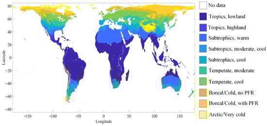
Figure 1.
Global Agro-Ecological Zones (GAEZ v4)-FAO.
Table 3.
Land cover/use clustering from the CCI legend (rows in red indicate classes with no SM retrievals).
2.3. Algorithms
In this research, two soil moisture retrieval methods were assessed, each expected to have different pros and cons. The inversion of a semiempirical forward model of GNSS-R reflectivity as a function of Earth surface parameters was expected to be more robust; in fact, especially at the beginning of the HydroGNSS mission the limited amount of training data could lead to overfitting of data-driven approaches. We also evaluated an ANN that is widely used in the literature and can effectively exploit auxiliary information and discover relationships with the target soil moisture. Therefore, the comparison considers the limits and strengths of each method. Based on these considerations, each algorithm was developed and evaluated to highlight its performance under different conditions, providing a comprehensive understanding of their strengths and weaknesses in the context of soil moisture estimation.
2.3.1. Semiempirical Model
The semiempirical method is rooted in the forward model proposed in [13]. The method involves two main steps: calibration of the forward model parameters and training of the inverse model. The dataset from August 2018 to July 2020 (two years) was divided (via sequential sampling) into two equal parts. Therefore, part one (P1) and part two (P2) were used in the forward and inverse training steps, respectively. Finally, the remaining portion of the dataset, from August 2020 to July 2021 (one year), was reserved as an independent dataset to validate the SM generated by the semiempirical method.
Utilizing the semiempirical forward model proposed in [13], the effective reflectivity () comes from a combination of coherent and incoherent scattering from the terrain, and attenuation and volume scattering from the vegetation and can be expressed as in Equation (3):
Here, is the incidence angle at the specular point, R is the Fresnel reflection coefficient (a function of soil moisture), SM is the soil moisture, is incoherent bistatic normalized radar cross section (BNRCS) of a homogeneous vegetated layer, is the vegetation optical depth; and is a bulk surface scattering parameter. S is a geometric factor that transforms the BNRCS into reflectivity by incorporating the spatial configuration of the radar system. The vegetation optical depth is expressed as a function of the incidence angle and the VOD from SMAP as . Then the and S parameters can be expressed by Equations (4) and (5):
In the above, is the roughness-dependent incoherent soil scattering term, and (scattering loss factor) accounts for the power loss of the coherent soil reflection caused by diffused scattering (where k is the wave number at L-band, and h is the small-scale surface roughness standard deviation). The parameter describes both small- and large-scale roughness effects. represents the horizontal discrimination area, which quantifies the effective scattering surface contributing to the received signal. The formulation of S considers the bistatic geometry and the different dependence of the distances of the ground target to the transmitter () and receiver ().
For model calibration, and were derived by fitting Equation (3) using the first part of the dataset (P1). The SMAP VOD provided , and the reflectivity was taken from CYGNSS observations. The Fresnel reflection coefficient was obtained via the Mironov dielectric constant model [41] using the SMAP-retrieved soil moisture. AFS is retrieved at each 25 km pixel whereas gamma is retrieved for each strata.
Once and are estimated (and assuming they can be considered time-invariant), soil moisture is retrieved by applying the regression formula in Equation (6) (with coefficients a, b, c, and d tuned using an independent set of SMAP data, namely the second part of the dataset P2). This equation assumes a linear relationship between the Fresnel reflectivity (in dB) and soil moisture:
This algorithm can be considered semiempirical, as it accounts for a functional relationship between observed reflectivity and bio-geophysical parameters taken from physical considerations but also enables the introduction of additional auxiliary information in the regression formula or different weights for predictive variables that are deemed useful for the inversion.
2.3.2. Artificial Neural Network (ANN)
The ANN is a data-driven approach that has been widely explored in the literature. In this paper, we follow the scheme proposed in [22]. The ANN model developed for soil moisture retrieval is a feed-forward multilayer perceptron developed through the Deep Learning Toolbox of the Matlab. More in-depth investigations are added to select the best dataset partition and combination of input features and to optimize the structure of the ANN. As a result of these assessments, the chosen network architecture is composed of 5 hidden layers with 18 neurons in each layer, using tansig activations and bias terms, while the output layer is a single linear neuron (purelin) suitable for regression. Weights were initialized with the Nguyen–Widrow scheme (initnw), and the model was trained with the Levenberg–Marquardt algorithm (trainlm).
Regarding the dataset partition, through an iterative process, it was decided to use 10% of the dataset for training and 90% for testing (from August 2018 to July 2020), so as to have a greater amount of data available during the testing phase and guarantee the model’s generalization. During the network training phase, the training dataset was then randomly divided into three parts (70%–15%–15% of the training data), according to the so-called early stopping rule, which also prevents the overfitting problem. Moreover, considerable effort was made to investigate the impact of different input combinations on retrieval performances.
Afterward, the remaining dataset covering August 2020 through July 2021 was designated as an independent dataset for validation purposes.
3. Results
In this section, the results are presented for SE and ANN models separately. Then, the models are evaluated and discussed together through a comparative analysis in Section 4.
3.1. Semiempirical
The fitting performance of the forward model was assessed by applying different data rejection rules based on the quality flags of SMAP and CYGNSS. Applying the Recommended Quality flag of SMAP removed 20–40% of data over land (varying by region, season, and environmental conditions). Applying more conservative quality flags slightly improves the accuracy of the forward model estimations at the cost of an increased number of missing pixels. Table 4 summarizes the performances of the forward model under different quality filtering. The density plot of Figure 2 shows the estimated reflectivity from the forward model versus the CYGNSS reflectivity when applying the SMAP Successful Retrieval quality flag.
Table 4.
Forward model performances with different SMAP quality controls.
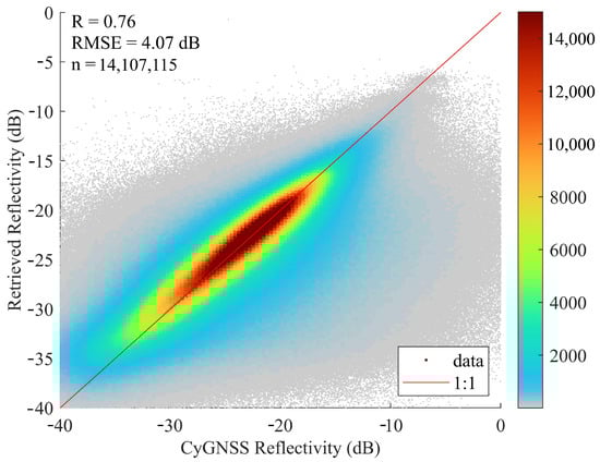
Figure 2.
Estimated reflectivity from forward model vs. CYGNSS reflectivity (with SMAP Successful Retrieval flag).
Figure 3 illustrates how filtering out data according to the Recommended Quality flag of SMAP affects the estimation of AFS, as well as that of at the cost of a significant increase in missing values, without improving the performance noticeably. In Figure 3 we also analyze the retrieved AFS as an indicator to account for surface roughness (the Retrieval Successful flag was used here). Indeed, a good correlation with the DEM elevation greater than 1000 m is observed, with a correlation coefficient ; there is also a correlation coefficient of with the DEM slope. It is worth recalling that the AFS parameter includes not only the effect of the large-scale roughness represented by the DEM, but also that of the wavelength-scale small surface roughness.
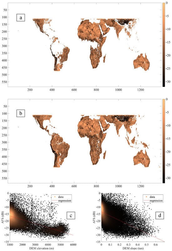
Figure 3.
Global AFS map at 25 km resolution (a) with SMAP Recommended Quality flag, (b) with SMAP Successful Retrieval flag, (c) AFS vs. DEM elevation > 1000 m, and (d) AFS vs. DEM slope.
Figure 4 shows the map of retrieved and scatter plots analyzing how it is correlated to the AGB. shows a good correlation with AGB for values greater than 50 Mg/ha (dense forests or woodlands), with a correlation coefficient .
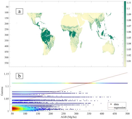
Figure 4.
(a) Global map at 25 km resolution with SMAP Successful Retrieval flag, (b) vs. AGB > 50 Mg/ha ().
Using the estimated AFS and from the forward model, the best-fitting coefficients a, b, c, and d in (4) were retrieved using the second part (P2) of the training set. The performance of the inversion is summarized in Table 5.
Table 5.
Inversion model performances with different SMAP quality controls.
The results indicate a trade-off between accuracy and correlation when comparing the SMAP Recommended Quality flag and the Successful Retrieval quality flag. While using the first flag achieves a significantly lower RMSE = 0.067 m3 m−3, the second flag exhibits a stronger correlation (0.82), suggesting better consistency of the retrieved SM with the reference SMAP data trend. Additionally, the Successful Retrieval quality flag results in fewer missing values. The density plots of Figure 5 show the retrieved SM versus the SMAP SM for the independent validation set under the two different SMAP flag filtering strategies.
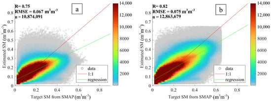
Figure 5.
Retrieved SM from semiempirical model vs. SMAP SM (a) with SMAP Recommended Quality flag, (b) with SMAP Successful Retrieval flag.
3.2. ANN
In the initial analysis, only CYGNSS variables (described in Section 2) served as inputs to the network. Subsequently, the configuration process entailed incorporating additional auxiliary variables as network inputs. After analyzing the CYGNSS-only case, terrain topography information, land cover classification, and vegetation-related variables were introduced as additional inputs. Topography variables include DEM elevation, SLOPE, and rmsHEIGHT. Vegetation indicators include AGB, SMAP-derived indices (VOD and VWC), and MODIS-derived indices (NDVI and NDWI). In general, as the number of network inputs increases, performance improves, as expected, since the augmented inputs offer the network more information to estimate the quantity closely aligned with the reference. Moreover, like the semiempirical approach, the accuracy of the ANN model was assessed under two different SMAP quality flags. Incorporating more quality flags improves the performance of the ANN model but leads to a greater number of missing pixels. Table 6 summarizes the ANN’s performance with different input sets under each SMAP quality flag criterion.
Table 6.
Performance of ANN with different inputs and applying different SMAP quality flags. CYGNSS variables in the table are Reflectivity_dB, SNR, , TE_WIDTH, index_c, Kurtosis.
The network capability was further investigated by applying the same stratification described in Section 3. Based on the results, the last input combination with the Successful Retrieval flag was chosen for the stratified analysis, as it exhibits the best compromise between acceptable model performance and fewer missing values. The only difference is that since the LCC contributes to stratification, it was removed from the network inputs. Using the stratification approach, the overall performance of the ANN model was slightly improved from 0.051 m3 m−3 to 0.047 m3 m−3. Figure 6 shows the scatter plot of estimated soil moisture vs. SMAP soil moisture with stratification versus without stratification. In the stratified estimation, the plot is a bit more scattered because of the limited number of points in some strata, but overall error metrics still improved slightly.
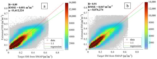
Figure 6.
Retrieved SM from ANN model vs. SMAP SM applying SMAP Successful Retrieval flag, (a) without stratification and (b) with stratification.
3.3. Validation Against ISMN Data
By comparing the SM estimated by the ANN and SE models with the in-situ SM derived from daily averaging the ISMN measurements available within each grid cell at a resolution of 25 km, the SM algorithm has been validated. Table 7 summarizes the findings in terms of R and RMSE.
Table 7.
Performance comparison of SMAP, ANN, and SE models across different stations using RMSE and correlation coefficient (R). Bold values indicate RMSE < 0.07 m3 m−3 and R > 0.7.
Figure 7 presents scatter plots comparing in situ soil moisture observations with estimates from SMAP, and from CYGNSS using the ANN, and the semiempirical (SE) algorithm across the OzNet and SCAN networks, including individual stations at Wynella, Crossroads, and Walnut Gulch. Overall, SMAP and ANN demonstrate comparable or superior performance to the SE model in most cases, with notable differences in correlation and error metrics across sites.
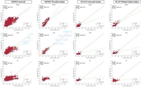
Figure 7.
Scatter plots comparing in situ soil moisture from ISMN with SMAP soil moisture, estimated soil moisture from ANN, and SE models across the OzNet network, Wynella station, and SCAN stations (Crossroads and Walnut Gulch).
Within the OzNet network, SMAP achieved a strong correlation (R = 0.71) and a moderate RMSE (0.075 m3 m−3), while the ANN exhibited a slightly lower correlation (R = 0.68) but a marginally improved RMSE (0.066 m3 m−3). At the station level, the Wynella site showed particularly high agreement between in situ and satellite/model estimates, with ANN outperforming all methods (R = 0.81, RMSE = 0.043 m3 m−3), followed closely by SMAP (R = 0.86, RMSE = 0.057 m3 m−3). In contrast, the SE model showed lower accuracy at Wynella (R = 0.46), consistent with its weaker performance across the network. For the SCAN stations, SMAP consistently performed better than the two CYGNSS algorithms in terms of correlation, especially at Walnut Gulch (R = 0.73), where ANN and SE showed lower agreement (R = 0.54 and 0.24, respectively). At Crossroads, both SMAP and ANN achieved similar performance (R , RMSE m3 m−3), while the SE model exhibited a low correlation (R = 0.4) and a higher RMSE (0.077 m3 m−3).
These results highlight the robustness of ANN-based estimates, particularly in agriculturally dominated and semi-arid regions like those covered by OzNet. However, SMAP remains competitive at the site scale, and its physically based retrieval approach offers more stable performance in sparsely vegetated environments such as Walnut Gulch. The SE model, while simpler, generally underperformed, especially in heterogeneous or dryland contexts.
4. Discussion
To interpret the results in a hydrologically and physically meaningful way, we examine patterns by land cover types under different climate (temperature) regimes. This stratified analysis reveals how vegetation characteristics and climate interact to affect model performance, consistent with known remote sensing limitations (e.g., vegetation attenuation) and soil moisture dynamics. Table 8 and Table 9 detail RMSEs and correlations across stratifications.
Table 8.
RMSE (m3 m−3) from ANN and SE models across land covers and climate zones. Bold values indicate RMSE < 0.07 m3 m−3. NaN means no quality-controlled data exist for the strata.
Table 9.
Correlation coefficient (R) results from ANN and SE models across land covers and climate zones. Bold values indicate R > 0.7. NaN means no quality-controlled data exist for the strata.
Performance varies by climate and land cover: tropical/subtropical zones show higher RMSEs and lower R. Vegetation density matters, where evergreen/deciduous forests have relatively high errors; barren and sparsely vegetated areas yield the lowest RMSEs and higher correlations. Cultivated and mixed systems are moderate, hinting at management effects. Subtropics exhibit the widest spread; temperate/boreal are more uniform with lower errors. Meadows, mosses, and lichens show mixed patterns, reflecting climate-dependent moisture retention. The comparison between the semiempirical model and the ANN model highlights significant differences in RMSE values across various land cover types and climate zones. Overall, the ANN model consistently outperforms the semiempirical model, as it produces lower RMSE values across nearly all climate regions.
Table 10 shows the number of available data for each strata, used in training models, and the percentage of improvement in performance, reduction in RMSE, by applying the ANN model.
Table 10.
Performance improvement (P.I., %) using ANN and number of samples (N, ) across land covers and climate zones. Bold values indicate P.I. and N (i.e., N in the table). NaN means no quality-controlled data exist for the strata.
For instance, in Cultivated land, Subtropics-cool, RMSE drops from 0.084 m3 m−3 (SE) to 0.047 m3 m−3 (ANN), an improvement of 44%. Likewise, Natural vegetation, Subtropics-warm sees RMSE reduced from 0.061 m3 m−3 to 0.034 m3 m−3 ( 44% reduction). These gains suggest that the ANN can model complex and non-linear relationships in the GNSS-R signals and auxiliary data that the semiempirical model cannot. However, the improvement in performance was not observed in all stratifications. In some cases, the ANN performs worse or no better than the semiempirical model (negative or near-zero improvement). Notable failures include Natural vegetation, Temperate-moderate, where RMSE doubled from 0.049 m3 m−3 in SE to 0.095 m3 m−3 in ANN (a –93.9% relative change) indicating a serious performance decline. Similarly, the Evergreen forest, Temperate-moderate experienced a RMSE rise from 0.073 m3 m−3 to 0.089 m3 m−3 in ANN (21.9% worse). These cases highlight that the ANN, despite its overall strength, can overfit or struggle in certain conditions. Possible causes include insufficient training data for that stratification or conditions (e.g., seasonal freeze/thaw or very uniform soil moisture) where the physical model’s simpler assumptions actually generalize better.
To better illustrate the differences in models’ performance, Figure 8 compares models’ performance in six representative stratifications. These examples were chosen to span a range of cover types and climates, highlighting scenarios of strong ANN improvement versus cases where both models struggle or perform similarly.
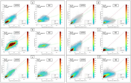
Figure 8.
Scatter plot of estimated soil moisture vs. SMAP soil moisture across six different stratifications: (a) Cultivated land—Subtropics, cool, (b) Evergreen forest—Subtropics, warm, (c) Spontaneous vegetation—Subtropics, moderately cool, (d) Natural vegetation—Subtropics, warm, (e) Barren areas—Subtropics, warm, (f) Meadows, mosses and lichens—Tropics, lowland.
In Figure 8, case a represents pixels classified as an agricultural region in a cooler subtropical climate. It exhibits a strong improvement with the ANN model. Quantitatively, the ANN achieves higher correlation (R = 0.84) and significantly lower RMSE (RMSE = 0.047 m3 m−3) than the SE (R = 0.63 and RMSE = 0.084 m3 m−3) here, reflecting one of the largest model skill gains observed. Such dramatic improvement suggests that in cultivated landscapes with moderate climate, the ANN can learn crop-specific and non-linear soil moisture responses (e.g., effects of irrigation or tillage) that a generic empirical model cannot. Case b shows weak gain from the ANN. Both models struggle under the closed canopy of an evergreen broadleaf forest. The scatter plot reveals that neither model predicts soil moisture with high precision. This is due to the fact that GNSS signals are heavily attenuated by the dense biomass and yield little sensitivity to soil moisture beneath [42]. We still note a higher correlation in the ANN model (R = 0.64) with respect to the SE model (R = 0.39). However, the overall performances are poor. This underlines that in dense forests, retrieval accuracy is fundamentally limited, and even large training datasets yield only incremental gains. It also exemplifies why global GNSS-R products tend to report higher errors in rain forest regions [42].
Spontaneous vegetation—Subtropics, moderately cool strata, case c, refers to areas of spontaneous vegetation (uncultivated, regenerating shrub/woodland or secondary growth) in a moderately cool subtropical climate. Here, we observe a moderate gain in ANN. The SE model’s scatter shows a fair amount of error—points deviate from the 1:1 line due to mixed land cover and seasonal climate influences that a simple model does not handle well. ANN predictions form a tighter cloud around the truth line, indicating improved accuracy. We interpret this as a middle-ground scenario: the subtropical mod. cool climate means the region likely experiences cooler seasons or elevation influences, and the spontaneous vegetation cover is semi-dense. These factors introduce complexity (e.g., periodic soil freeze/thaw or variable canopy density) that the ANN only partially learns from the available data. There is still error reduction relative to SE. The result is a noticeable, though not extreme, improvement, for example, correlation raised from 0.55 to 0.81 and RMSE drop accordingly from 0.087 to 0.071. This case exemplifies an intermediate performance regime, where the ANN confers a benefit but underlying challenges (mixed vegetation and climate variability) limit just how much improvement is achievable. Stratification in d involves an open natural vegetation area (e.g., savanna or grassland) in a warm subtropical climate, where the ANN shows a great boost in performance, from R = 0.48 to R = 0.86 and RMSE = 0.061 m3 m−3 to RMSE = 0.034 m3 m−3. The SE model already performs reasonably well here (since vegetation is not continuous), but its linear assumptions falter in capturing certain moisture dynamics. The ANN fits the data much more closely. In the scatter plot, ANN predictions tightly cluster along the 1:1 line, indicating high accuracy, whereas SE predictions exhibit noticeable bias and dispersion. This strong ANN gain likely arises because open natural ecosystems present complex but learnable patterns; soil moisture responds to rainfall pulses and dries out with a timing influenced by light vegetation cover. The ANN can integrate these patterns (by implicitly accounting for factors like vegetation indices), whereas the semiempirical model leaves systematic errors.
Barren areas and Subtropics-warm strata, case e, highlights a warm subtropical barren area (or very sparse vegetation), a regime where both models are highly effective and achieved low RMSEs. The ANN performed slightly better than the SE model. However, the improvement is marginal because the problem is already well-constrained by the physics of the environment. In bare soil, GNSS reflectivity has a strong, direct relationship to moisture (high signal-to-noise), which a simple linear model can capture fairly well. Finally, case f represents a tropical lowland regime characterized by meadows, mosses, and lichens land cover. In this strata, we found the highest performance improvement, 47.2% reduction in RMSE from 0.072 m3 m−3 to 0.038 m3 m−3. Again, the results highlight the ANN’s advantage in environments where the soil–moisture signal is partially obscured or distorted by biophysical layers. In such conditions, the flexibility of machine learning proves essential, capturing nuanced variations that exceed the capacity of simple empirical or linear models.
Moreover, a perspective is given by the ratio of RMSE and standard deviation () of soil moisture, which normalizes error by the natural variability of soil moisture in each stratification. In [43], authors argued for providing additional context like the standard deviation of observed data along with error measures, to avoid misinterpretation of RMSE in isolation. This recommendation laid the groundwork for using the RMSE/ ratio, ensuring that model error is judged relative to natural variability in the data. A ratio below 1.0 means the model error is smaller than the soil moisture’s standard deviation (indicating the model has skill beyond predicting the mean), whereas ratio indicates the model performs worse than a simple mean-value baseline. The semiempirical model’s ratio exceeds 1 in most stratification, often the 1.1–1.5 range, even in some dry cases. The ANN model dramatically improves these ratios in most cases, often bringing them well below 1. For instance, in Cultivated, Subtropics-mod. cool the ratio drops from 1.25 (SE) to 0.72 (ANN), and in Deciduous forest, Tropics-lowland from 1.12 to 0.66. Such reductions mean the ANN is capturing a significant portion of the soil moisture variance that the semiempirical model missed. Table 11 summarizes the normalized RMSE for different stratification.
Table 11.
Normalized RMSE for ANN and SE models across land covers and climate zones. NaN means no quality-controlled data exist for the strata.
As shown in Table 11, Figure 9 provides global maps of SMAP soil moisture standard deviation and the spatial distribution of normalized RMSE for both ANN and SE models. These maps further confirm that the ANN outperforms the SE model in most regions, especially where natural variability is high and nonlinear patterns dominate. Areas where normalized RMSE > 1 indicate regimes where the model fails to capture the full dynamics of soil moisture.
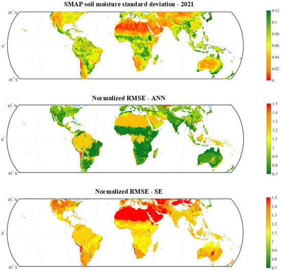
Figure 9.
Global maps showing the standard deviation of SMAP soil moisture estimates (std) over the study year 2021, and the normalized RMSE (RMSE/std) of the ANN and SE models. These maps highlight regional differences in model performance relative to natural soil moisture variability.
Overall, the ANN outperforms the semi-empirical (SE) model in most climate–land-cover combinations where non-linear responses dominate. Conversely, the SE approach performs on par with the ANN in well-constrained regimes (e.g., bare soil or homogeneous croplands) where almost a linear reflectivity–moisture relation holds. These patterns indicate that ANN advantages emerge precisely where signal–environment interactions are complex and non-linear, whereas the SE model remains a strong, interpretable baseline in simpler regimes. Moreover, both approaches degrade where training data are scarce (e.g., high latitude/cold regimes with limited CyGNSS coverage). In such under-sampled strata, the ANN’s advantage narrows and occasional instabilities appear, underscoring that data availability, not only model choice, constrains retrieval skill in these regions.
One practical benefit of an ANN-based retrieval system is that it can retain high accuracy even when data quality filtering is less strict. Compared to the SE technique, it may therefore utilize a greater number of GNSS-R observations without sacrificing performance, which is an important advantage for the ESA HydroGNSS mission, which aims to maximize data utilization. Both methods, however, performed worse in areas with very little training data (such as high-latitudes) where CyGNSS coverage was limited. This result emphasizes that a significant number of the existing performance gaps in these under-sampled regions (such as boreal climates) are mostly caused by a lack of observations. The upcoming HydroGNSS mission will help mitigate this issue by extending GNSS-R measurements to higher latitudes and providing additional data for model training and validation in these challenging environments.
5. Conclusions
This study demonstrates that an ANN-based approach can significantly improve the accuracy of soil moisture retrieval from CyGNSS reflectometry data compared to a semiempirical (SE) model. The ANN achieved consistently lower retrieval errors and higher correlations across most of climate–land cover stratifications. ANN has the advantage in complex, heterogeneous environments where nonlinear interactions affect the GNSS-R signal. Conversely, the SE algorithm performed similar to the ANN in straightforward conditions (e.g., bare soil or uniform croplands). Overall, these findings demonstrate that the ANN approach is the best option for GNSS-R soil moisture estimate, while also demonstrating that the SE model continues to function well in settings with strict constraints that are consistent with its underlying hypotheses. Therefore, a hybrid retrieval approach that builds on the complementary advantages of both approaches can be suggested for further research. To enhance more soil moisture retrieval performance, it will also be crucial to find more high-quality training data, particularly in underrepresented areas, and investigate cutting-edge machine learning approaches.
Author Contributions
Conceptualization, H.I., N.P., E.S. and L.G.; methodology, H.I., E.S., N.P. and L.G.; software, H.I., F.C., V.A. and L.C.; validation, H.I. and N.P.; formal analysis, H.I., E.S. and F.C.; investigation, H.I., E.S. and L.G.; resources, N.P., E.S. and L.G.; data curation, H.I. and F.C.; writing—original draft preparation, H.I.; writing—review and editing, H.I., E.S., F.C., L.G., L.C., V.A. and N.P.; visualization, H.I., F.C. and N.P.; supervision, N.P.; project administration, N.P.; funding acquisition, N.P. and E.S. All authors have read and agreed to the published version of the manuscript.
Funding
This research received no external funding.
Data Availability Statement
The data and the code of this study are available from the corresponding author upon request.
Acknowledgments
The authors would like to thank the European Space Agency (ESA) for supporting the HydroGNSS mission development. H.I. gratefully acknowledges the support of the PhD program in the National PhD program in Earth Observation at Sapienza University of Rome.
Conflicts of Interest
The authors declare no conflict of interest.
References
- Entekhabi, D.; Njoku, E.G.; O’Neill, P.E.; Kellogg, K.H.; Crow, W.T.; Edelstein, W.N.; Entin, J.K.; Goodman, S.D.; Jackson, T.J.; Johnson, J.; et al. The soil moisture active passive (SMAP) mission. Proc. IEEE 2010, 98, 704–716. [Google Scholar] [CrossRef]
- Kerr, Y.H.; Waldteufel, P.; Wigneron, J.P.; Martinuzzi, J.M.; Font, J.; Berger, M. Soil moisture retrieval from space: The Soil Moisture and Ocean Salinity (SMOS) mission. IEEE Trans. Geosci. Remote Sens. 2001, 39, 1729–1735. [Google Scholar] [CrossRef]
- Zavorotny, V.U.; Gleason, S.; Cardellach, E.; Camps, A. Tutorial on remote sensing using GNSS bistatic radar of opportunity. IEEE Geosci. Remote Sens. Mag. 2014, 2, 8–45. [Google Scholar] [CrossRef]
- Ruf, C.S.; Unwin, M.; Dickinson, J.; Rose, R.; Rose, D.; Vincent, M.A.; Lyons, A.; Gleason, S.; Jelenak, Z.; Said, F.; et al. New Ocean Winds Satellite Mission to Probe Hurricanes and Tropical Convection. Bull. Am. Meteorol. Soc. 2016, 97, 385–395. [Google Scholar] [CrossRef]
- Pierdicca, N.; Guerriero, L.; Giusto, R.; Brogioni, M.; Egido, A. SAVERS: A simulator of GNSS reflections from bare and vegetated soils. IEEE Trans. Geosci. Remote Sens. 2014, 52, 6542–6554. [Google Scholar] [CrossRef]
- Chew, C.C.; Small, E.E.; Larson, K.M.; Zavorotny, V.U. Effects of near-surface soil moisture on GPS SNR data: Development of a retrieval algorithm for soil moisture. IEEE Trans. Geosci. Remote Sens. 2014, 52, 537–543. [Google Scholar] [CrossRef]
- Chew, C.C.; Small, E.E. Soil Moisture Sensing Using Spaceborne GNSS Reflections: Comparison of CYGNSS Reflectivity to SMAP Soil Moisture. Geophys. Res. Lett. 2018, 45, 4049–4057. [Google Scholar] [CrossRef]
- Clarizia, M.P.; Pierdicca, N.; Costantini, F.; Floury, N. Analysis of cygnss data for soil moisture retrieval. IEEE J. Sel. Top. Appl. Earth Obs. Remote Sens. 2019, 12, 2227–2235. [Google Scholar] [CrossRef]
- Guerriero, L.; Martín, F.; Mollfulleda, A.; Paloscia, S.; Pierdicca, N.; Santi, E.; Floury, N. Ground-Based Remote Sensing of Forests Exploiting GNSS Signals. IEEE Trans. Geosci. Remote Sens. 2020, 58, 6844–6860. [Google Scholar] [CrossRef]
- Pierdicca, N.; Comite, D.; Camps, A.; Carreno-Luengo, H.; Cenci, L.; Clarizia, M.P.; Costantini, F.; Dente, L.; Guerriero, L.; Mollfulleda, A.; et al. The Potential of Spaceborne GNSS Reflectometry for Soil Moisture, Biomass, and Freeze-Thaw Monitoring: Summary of a European Space Agency-funded study. IEEE Geosci. Remote Sens. Mag. 2022, 10, 8–38. [Google Scholar] [CrossRef]
- Azemati, A.; Melebari, A.; Campbell, J.D.; Walker, J.P.; Moghaddam, M. GNSS-R Soil Moisture Retrieval for Flat Vegetated Surfaces Using a Physics-Based Bistatic Scattering Model and Hybrid Global/Local Optimization. Remote Sens. 2022, 14, 3129. [Google Scholar] [CrossRef]
- Setti, P.T.; Tabibi, S. Evaluation of Spire GNSS-R reflectivity from multiple GNSS constellations for soil moisture estimation. Int. J. Remote Sens. 2023, 44, 6422–6441. [Google Scholar] [CrossRef]
- Yueh, S.H.; Shah, R.; Chaubell, M.J.; Hayashi, A.; Xu, X.; Colliander, A. A Semiempirical Modeling of Soil Moisture, Vegetation, and Surface Roughness Impact on CYGNSS Reflectometry Data. IEEE Trans. Geosci. Remote Sens. 2022, 60, 1–17. [Google Scholar] [CrossRef]
- Bu, J.; Wang, Q.; Wang, Z.; Fan, S.; Liu, X.; Zuo, X. Land Remote Sensing Applications Using Spaceborne GNSS Reflectometry: A Comprehensive Overview. IEEE J. Sel. Top. Appl. Earth Obs. Remote Sens. 2024, 17, 12811–12841. [Google Scholar] [CrossRef]
- Asgarimehr, M.; Entekhabi, D.; Camps, A. Diurnal Vegetation Moisture Cycle in the Amazon and Response to Water Stress. Geophys. Res. Lett. 2024, 51, e2024GL111462. [Google Scholar] [CrossRef]
- Setti, P.; Tabibi, S. Comprehensive Analysis of CYGNSS GNSS-R Data for Enhanced Soil Moisture Retrieval. IEEE J. Sel. Top. Appl. Earth Obs. Remote Sens. 2025, 18, 663–679. [Google Scholar] [CrossRef]
- Zhao, D.; Asgarimehr, M.; Heidler, K.; Wickert, J.; Zhu, X.X.; Mou, L. Deep Learning-Based GNSS-R Global Vegetation Water Content: Dataset, Estimation, and Uncertainty. IEEE J. Sel. Top. Appl. Earth Obs. Remote Sens. 2025, 18, 17386–17404. [Google Scholar] [CrossRef]
- Song, S.; Zhu, Y.; Qu, X.; Tao, T. Spaceborne GNSS-R for Sensing Soil Moisture Using CYGNSS Considering Land Cover Type. Water Resour. Manag. 2025, 39, 3499–3519. [Google Scholar] [CrossRef]
- Al-Khaldi, M.M.; Johnson, J.T.; O’Brien, A.J.; Balenzano, A.; Mattia, F. Time-Series Retrieval of Soil Moisture Using CYGNSS. IEEE Trans. Geosci. Remote Sens. 2019, 57, 4322–4331. [Google Scholar] [CrossRef]
- Carreno-Luengo, H.; Luzi, G.; Crosetto, M. Above-Ground Biomass Retrieval over Tropical Forests: A Novel GNSS-R Approach with CyGNSS. Remote Sens. 2020, 12, 1368. [Google Scholar] [CrossRef]
- Eroglu, O.; Kurum, M.; Boyd, D.; Gurbuz, A.C. High Spatio-Temporal Resolution CYGNSS Soil Moisture Estimates Using Artificial Neural Networks. Remote Sens. 2019, 11, 2272. [Google Scholar] [CrossRef]
- Santi, E.; Clarizia, M.P.; Comite, D.; Dente, L.; Guerriero, L.; Pierdicca, N.; Floury, N. Combining Cygnss and Machine Learning for Soil Moisture and Forest Biomass Retrieval in View of the ESA Scout Hydrognss Mission. In Proceedings of the IGARSS 2022—2022 IEEE International Geoscience and Remote Sensing Symposium, Kuala Lumpur, Malaysia, 17–22 July 2022; pp. 7433–7436. [Google Scholar] [CrossRef]
- Santi, E.; Comite, D.; Dente, L.; Guerriero, L.; Pierdicca, N.; Clarizia, M.P.; Floury, N. Global soil moisture mapping at 5 km by combining GNSS reflectometry and machine learning in view of HydroGNSS. Sci. Remote Sens. 2024, 10, 100177. [Google Scholar] [CrossRef]
- Campbell, J.D.; Akbar, R.; Azemati, A.; Bringer, A.; Comite, D.; Dente, L.; Gleason, S.T.; Guerriero, L.; Hodges, E.; Johnson, J.T.; et al. Intercomparison of Models for CYGNSS Delay-Doppler Maps at a Validation Site in the San Luis Valley of Colorado. In Proceedings of the 2021 IEEE International Geoscience and Remote Sensing Symposium IGARSS, Brussels, Belgium, 11–16 July 2021; pp. 2001–2004. [Google Scholar] [CrossRef]
- Yang, C.; Mao, K.; Guo, Z.; Shi, J.; Bateni, S.M.; Yuan, Z. Review of GNSS-R Technology for Soil Moisture Inversion. Remote Sens. 2024, 16, 1193. [Google Scholar] [CrossRef]
- Unwin, M.J.; Pierdicca, N.; Cardellach, E.; Rautiainen, K.; Foti, G.; Blunt, P.; Guerriero, L.; Santi, E.; Tossaint, M. An Introduction to the HydroGNSS GNSS Reflectometry Remote Sensing Mission. IEEE J. Sel. Top. Appl. Earth Obs. Remote Sens. 2021, 14, 6987–6999. [Google Scholar] [CrossRef]
- Gleason, S.; O’Brien, A.; Russel, A.; Al-Khaldi, M.M.; Johnson, J.T. Geolocation, Calibration and Surface Resolution of CYGNSS GNSS-R Land Observations. Remote Sens. 2020, 12, 1317. [Google Scholar] [CrossRef]
- Pascual, D.; Clarizia, M.P.; Ruf, C.S. Spaceborne Demonstration of GNSS-R Scattering Cross Section Sensitivity to Wind Direction. IEEE Geosci. Remote Sens. Lett. 2022, 19, 1–5. [Google Scholar] [CrossRef]
- Carreno-Luengo, H.; Lowe, S.; Zuffada, C.; Esterhuizen, S.; Oveisgharan, S. Spaceborne GNSS-R from the SMAP Mission: First Assessment of Polarimetric Scatterometry over Land and Cryosphere. Remote Sens. 2017, 9, 362. [Google Scholar] [CrossRef]
- Al-Khaldi, M.M.; Johnson, J.T.; Gleason, S.; Loria, E.; O’Brien, A.J.; Yi, Y. An Algorithm for Detecting Coherence in Cyclone Global Navigation Satellite System Mission Level-1 Delay-Doppler Maps. IEEE Trans. Geosci. Remote Sens. 2021, 59, 4454–4463. [Google Scholar] [CrossRef]
- ESA Land Cover CCI Project Team. ESA CCI Land Cover—Annual Global Land Cover Maps (1992–2015), Version 2.0.7. 2017. Available online: https://climate.esa.int/en/projects/land-cover/ (accessed on 13 October 2025).
- U.S. Geological Survey, EROS Center. GTOPO30 Readme; Technical report; U.S. Geological Survey: Sioux Falls, SD, USA, 2018.
- Dorigo, W.A.; Wagner, W.; Hohensinn, R.; Hahn, S.; Paulik, C.; Xaver, A.; Gruber, A.; Drusch, M.; Mecklenburg, S.; Oevelen, P.V.; et al. The International Soil Moisture Network: A data hosting facility for global in situ soil moisture measurements. Hydrol. Earth Syst. Sci. 2011, 15, 1675–1698. [Google Scholar] [CrossRef]
- Dorigo, W.A.; Xaver, A.; Vreugdenhil, M.; Gruber, A.; Hegyiová, A.; Sanchis-Dufau, A.D.; Zamojski, D.; Cordes, C.; Wagner, W.; Drusch, M. Global Automated Quality Control of In Situ Soil Moisture Data from the International Soil Moisture Network. Vadose Zone J. 2013, 12, 1–21. [Google Scholar] [CrossRef]
- Ruf, C.S. Chapter 10—Level 3 Soil Moisture Product. In CYGNSS Handbook, 2nd ed.; University of Michigan/NASA CYGNSS Mission: Ann Arbor, MI, USA, 2022; Chapter 10. [Google Scholar] [CrossRef]
- Chan, S.; Dunbar, R.S. Soil Moisture Active Passive (SMAP) Mission Level 3 Passive Soil Moisture Product Specification Document Version 8.0 R18 Release; Jet Propulsion Laboratory, California Institute of Technology: Pasadena, CA, USA, 2021; JPL D-72551. [Google Scholar]
- Goward, S.N.; Xue, Y.; Czajkowski, K.P. Evaluating land surface moisture conditions from the remotely sensed temperature/vegetation index measurements: An exploration with the simplified simple biosphere model. Remote Sens. Environ. 2002, 79, 225–242. [Google Scholar] [CrossRef]
- Pablos, M.; Piles, M.; Sanchez, N.; Gonzalez-Gambau, V.; Vall-Llossera, M.; Camps, A.; Martinez-Fernandez, J. A sensitivity study of land surface temperature to soil moisture using in-situ and spaceborne observations. In Proceedings of the 2014 IEEE Geoscience and Remote Sensing Symposium, Quebec City, QC, Canada, 13–18 July 2014; pp. 3267–3269. [Google Scholar] [CrossRef]
- Noguera, I.; Vicente-Serrano, S.M.; Peña-Angulo, D.; Domínguez-Castro, F.; Juez, C.; Tomás-Burguera, M.; Lorenzo-Lacruz, J.; Azorin-Molina, C.; Halifa-Marín, A.; Fernández-Duque, B.; et al. Assessment of vapor pressure deficit variability and trends in Spain and possible connections with soil moisture. Atmos. Res. 2023, 285, 106666. [Google Scholar] [CrossRef]
- Fischer, G.; Nachtergaele, F.O.; van Velthuizen, H.; Chiozza, F.; Franceschini, G.; Henry, M.; Muchoney, D.; Tramberend, S. Global Agro-Ecological Zones (GAEZ v4)—Model Documentation; Technical Report; Food and Agriculture Organization of the United Nations (FAO): Rome, Italy; IIASA: Laxenburg, Austria, 2021. [Google Scholar] [CrossRef]
- Mironov, V.L.; Kosolapova, L.G.; Fomin, S.V. Physically and mineralogically based spectroscopic dielectric model for moist soils. IEEE Trans. Geosci. Remote Sens. 2009, 47, 2059–2070. [Google Scholar] [CrossRef]
- Liu, Q.; Zhang, S.; Li, W.; Nan, Y.; Peng, J.; Ma, Z.; Zhou, X.; Xu, J.; Bai, W.; Liu, Q.; et al. Using Robust Regression to Retrieve Soil Moisture from CyGNSS Data. Remote Sens. 2023, 15, 3669. [Google Scholar] [CrossRef]
- Moriasi, D.N.; Arnold, J.G.; Liew, M.W.V.; Bingner, R.L.; Harmel, R.D.; Veith, T.L. Model Evaluation Guidelines for Systematic Quantification of Accuracy in Watershed Simulations. Trans. ASABE 2007, 50, 885–900. [Google Scholar] [CrossRef]


Disclaimer/Publisher’s Note: The statements, opinions and data contained in all publications are solely those of the individual author(s) and contributor(s) and not of MDPI and/or the editor(s). MDPI and/or the editor(s) disclaim responsibility for any injury to people or property resulting from any ideas, methods, instructions or products referred to in the content. |
© 2025 by the authors. Licensee MDPI, Basel, Switzerland. This article is an open access article distributed under the terms and conditions of the Creative Commons Attribution (CC BY) license (https://creativecommons.org/licenses/by/4.0/).