Highlights
What are the main findings?
- Denoising is needed to enhance the performance and the coverage of the future ODYSEA mission.
- Neural network denoising (with a UNet) achieves better performance than classical smoothing on radial velocities.
What is the implication of the main finding?
- Smaller scales (up to 30 km in strong wind conditions) can be observed after UNet denoising.
- The UNet enables the reconstruction of the main eddies and fronts in the relative vorticity field.
Abstract
The ODYSEA (Ocean DYnamics and Surface Exchange with the Atmosphere) mission will provide simultaneous two-dimensional measurements of currents and winds for the first time. According to the ODYSEA radar concept, with a high incidence angle, current noise is primarily driven by backscattered power, which is triggered by wind speed. Therefore, random noise will affect the quality of observations. In low wind conditions, the absence of surface roughness increases the noise level considerably, to the point where the measurement becomes unusable, as the error can exceed 3 m/s at 5 km posting compared to mean current amplitudes of tens of cm/s. Winds higher than 7.5 m/s enable current measurements at 5 km posting with an RMS accuracy below 50 cm/s, but derivatives of currents will amplify noise, hampering the understanding of ocean dynamics and the interaction between the ocean and the atmosphere. In this context, this study shows the advantages and limitations of using noise-reduction algorithms. A convolutional neural network, a UNet inspired by the work of the SWOT (Surface Water and Ocean Topography) mission, is trained and tested on simulated radial velocities that are representative of the global ocean. The results are compared with those of classical smoothing: an Adaptive Gaussian Smoother whose filtering transfer function is optimized based on local wind speed (e.g., more smoothing in regions of low wind). The UNet outperforms the kernel smoother everywhere with our simulated dataset, especially in low wind conditions (SNR << 1) where the smoother essentially removes all velocities whereas the UNet mitigates random noise while preserving most of the signal of interest. Error is reduced by a factor of 30 and structures down to 30 km are reconstructed accurately. The UNet also enables the reconstruction of the main eddies and fronts in the relative vorticity field. It shows good robustness and stability in new scenarios.
1. Introduction
The interaction between winds and ocean currents plays an important role in ocean circulation [1]. To better understand this interaction and associated phenomena, a new satellite called ODYSEA (Ocean DYnamics and Surface Exchange with the Atmosphere) has been proposed for NASA’s Earth System Explorers Program. It is a joint mission between the Jet Propulsion Laboratory (JPL) and the Centre National d’Études Spatiales (CNES). The ODYSEA mission has four science objectives (https://cnes.fr/en/projects/odysea, accessed on 26 October 2025):
- Gain new insights into ocean–atmosphere climate forecasting and projections and improve climate projections.
- Understand how current wind coupling affects the main ocean currents, local and remote winds, and storm tracks.
- Understand how surface currents exchange and transport energy.
- Develop a deeper understanding of climate.
To achieve these goals, ODYSEA will measure winds and ocean currents simultaneously using a Doppler scatterometer [2,3]. It will provide a ~1500 km wide swath of coverage with a resolution of 5 km.
The Doppler scatterometer concept was first used during airborne campaigns [4] and shows promising results. It measures the radial velocities at the fore and the aft of a platform (see Figure 1 and for more details on the measurement principle (see [2])). From these radial velocities, eastward and northward velocities are derived. In order to measure radial velocities, ODYSEA will implement a monostatic pulsed radar in a Ka band mounted on a platform which rotates at 12 RPM. The phase difference of consecutive pulses yields a Doppler estimation of each range gate. After subtracting the non-geophysical Doppler due to movement of the satellite between two pulses, the radial velocities are retrieved for all possible azimuths, enabling fore/aft 2D reconstruction. Due to the high incidence angle of 56°, the radar backscatter from the sea surface is caused by capillary waves, whose wavelength (of ~5 mm) is in resonance with the radar wavelength in the Bragg regime. These capillary waves are very responsive to surface wind speed so that the measured backscatter power enables wind retrieval simultaneously. Moreover, the high incidence angles enable a very large swath of 1500 km. The drawback is weak SNR in very low wind regimes (<~5 m/s) which induces random noise on the radial currents [2,5,6]. In light wind conditions, the intensity of the noise is one order of magnitude greater than the signal of interest, if not more: the current measurements are lost in the noise and cannot be processed raw. For winds higher than 7.5 m/s, the noise level will be below 50 cm/s RMS, but it will affect derivative variables that are useful to oceanographers (vorticity, divergence…). Another caveat arises from fore/aft 2D inversion (see Figure 1): when looking purely along-track (resp. across-track), the fore and aft lines of sight are parallel, which increases the noise in the ill-conditioned across-track (resp. along-track) direction and prevents the full swath from fulfilling the mission requirements. Indeed, azimuths between 15° and 75° are considered non-exploitable. Therefore, we propose using noise-reduction algorithms in order to broaden the number of exploitable measurements, especially in low wind regimes and near the center and edge of the swath.
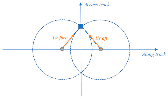
Figure 1.
Schematic diagram of the ODYSEA measurement. The Doppler scatterometer on board describes circles along its trajectory (dotted circles). Each intersection of two circles (blue square) defines a forward radial velocity (ur fore) and an afterward radial velocity (ur aft). By reprojecting these radial velocities, the northward and eastward velocities are deduced. Figure provided by CNES.
As random noise mitigation is a classic problem in image processing, many denoising algorithms have been developed: from statistical methods (e.g., Lanczos smoother, Gaussian smoother) to methods based on convolutional neural networks. Some of these have been compared in [7,8] in order to denoise the sea surface height anomalies provided by the SWOT (Surface Water and Ocean Topography) satellite [9]. The best results are obtained by a UNet, a convolutional neural network, trained on simulated SWOT data [8,10]. Indeed, this network has been selected for its robustness to different types of noise, its stability and its computation time.
The prescribed noise level is sufficient to meet the mission’s goals. However, for many applications, reducing the noise level is beneficial. Denoising would, for example, allow greater spatial coverage (i.e., access to velocities impacted by high noise levels) or access to smaller scales of the ocean. To achieve this, the UNet developed for SWOT is adapted to the specific geometry of ODYSEA and will be trained to denoise radial velocities. The performance and robustness of the UNet are also evaluated. A comparison is also made with an Adaptive Gaussian Smoother. The paper is organized as follows: Section 2 presents the data generated by the ODYSEA simulator. Then, Section 3 and Section 4 present the UNet and the metrics used to evaluate the performance, respectively. The results of the denoising and the performance are shown in Section 4. The last section shows the robustness of the UNet when it encounters degraded conditions.
2. Input Data
The input dataset is generated by the ODYSEA simulator (https://github.com/awineteer/odysea-science-simulator, accessed on 26 October 2025) which was modified by [11] with respect to orbital and noise models for different experimental configurations [2] and to provide Level 2 realistic measurements. The simulator interpolates an ocean model to reproduce Level 2 observations of ODYSEA. The model used is the Massachusetts Institute of Technology general circulation model (MITgcm LLC2160-C1440 configuration). It is coupled to an atmospheric model (Goddard Earth Observing System) and includes tidal forcing. Surface currents and winds variable at 10 m heights are used as input for the simulator. Their spatial and temporal resolution are 2–4 km and 1 h. Further information about the MITgcm is available at https://www.nas.nasa.gov/SC21/research/project16.html (accessed on 26 October 2025).
The dataset provides [5]
- Parameters of the satellite observations such as the along-track and cross-track distance and different observation angles.
- Physical variables interpolated from the MITgcm (wind speed and direction, eastward/northward velocities and radial velocities).
- Random errors that impact the radial velocities. The wind-dependent and the azimuth-dependent noise model is derived from Rodríguez et al. [2].
All variables are available at 5 km resolution. The project has simulated several noise models for different instrument and mission designs [11]. The datasets are available on the Aviso website: https://www.aviso.altimetry.fr/en/data/products/value-added-products/simulated-level-2-odysea-dataset.html (accessed on 26 October 2025). For all of them, the noise is random and depends on the wind speed and on the across-track distance (Figure 2). The lower the wind speed is, the higher the noise level is. These noise configurations do not consider the orientation of the wind, which will also affect the noise magnitude. All the random errors are specified by the project, but none of the configurations are representative of the final instrument and mission design. For this study, the E2 noise configuration referenced in [5], called hereafter the high-SNR configuration, is chosen. This corresponds to the parameters presented in Table 1 and to the noise level shown in Figure 2. Another design referenced in [5] as F configuration will be called hereafter the low-SNR configuration.
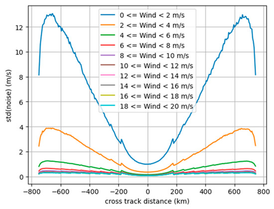
Figure 2.
Radial current noise as a function of cross-track distance and windspeed for the E2 configuration.

Table 1.
Summary of the high-SNR E2 and low-SNR F configurations available on Aviso. Table extracted from [5].
The dataset is available from February 2020 to January 2021 over the global ocean. Data in February 2020 is used for the training part. The rest of the dataset is used for the inference part.
3. Noise-Reduction Algorithms
3.1. Neural Network Method: UNet
The neural network method used is a UNet. This convolutional neural network has demonstrated good performances in various applications such as denoising [12,13], segmentation [14] or nowcasting [15]. Its structure is composed of two parts: an encoder which creates a compact representation of the input and a decoder which reconstructs the input without non-essential information such as noise. The encoder and the decoder are composed of convolutional blocks, which allow spatial information to be taken into account. The UNet used in this study is inspired by the one used to denoise SWOT data in [8]. Tréboutte et al. [8] and Dibarboure et al. [10] showed that the UNet is robust to different levels and types of noise (correlated noise). Its stability, light architecture and very low computation time for the inference part are its main advantages.
Noisy radial velocities (ur_fore and ur_aft variables) are used as inputs for the denoising algorithm. No normalization is applied to the radial velocities because it introduces a bias into the denoised data (Appendix A). Adding the wind speed as a third input was tested but this did not significantly improve the results (Appendix A). As a neural network requires data with a constant shape, each ODYSEA track is divided into 6400 km along-track. Thus, the input data images have a shape of 300 × 1280 pixels.
The two channels, i.e., the two components of the radial velocities, are trained together. The information is transferred from one channel to the other, i.e., the geometric relationship between the aft and fore components is implicitly built into the UNet during the training phase (Figure 1). This improves the performance compared to two separate trainings with only one input each (Appendix A). The learning method used is a supervised training: the outputs (i.e., the denoised radial velocities) are compared to the ground truth, which is the true radial velocities (ur_nonoise_fore and ur_nonoise_aft variables), thanks to an L1-loss function. UNet hyperparameters were tuned for our study and the UNet is composed of approximately 231,000 parameters.
3.2. Adaptive Gaussian Smoother
To compare the performance of the neural network, a Gaussian Smoother was also used to denoise radial velocities. As noise amplitude is highly variable with wind speed (large noise at low wind speeds and small noise at high wind speeds), the smoother needs to be adaptive according to wind speeds. Therefore, the optimal standard deviation (σ) of the Gaussian kernel is determined for each wind speed value. To achieve this, a sensitivity analysis of the Gaussian Smoother is carried out by varying the wind speed and σ. For each pair (wind speed, σ), the smoother is compared to the ground truth thanks to a Root Mean Square Error (RMSE). The optimal wind speed and σ correspond to the minimum of RMSE (Figure 3). To simplify the problem, σ is used as an integer between 1 and 14 and the wind speed is tabulated in order to work with ‘categories’. Table 2 shows the value of the optimal σ as a function of the wind speed. As expected, higher values of σ are suitable for low wind speeds and vice versa. For winds lower than 3 m/s, there is no minimum visible in Figure 3a. Indeed, the minimum of RMSE tends towards infinity, which means that an infinitely large kernel would be needed to filter areas affected by a high level of noise. However, σ is set up to 8 to avoid significant discontinuities with the category of winds between 3 and 4 m/s.
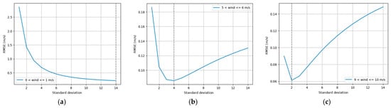
Figure 3.
RMSE as a function of the standard deviation of the Gaussian kernel for (a) winds between 0 and 1 m/s, (b) winds between 5 and 6 m/s and (c) winds between 9 and 10 m/s. The vertical dashed line corresponds to the minimum of RMSE.
Table 2.
Optimal standard deviation in pixels and in km of the Gaussian kernel as a function of wind speeds. One pixel corresponds to 5 km.
This adaptive smoother is not optimal and can be improved. Indeed, the variability of the ocean and the cross-track distance could be added as input parameters. Its objective is to provide a simple smoother that can be a baseline against which the UNet can be compared. This smoother behaves similarly to an optimal interpolation [16,17].
3.3. Computation Efficiency
The neural network was trained using an NVIDIA A100 GPU (from NVIDIA corporation, Santa Clara, United States), which is available for high-performance computing and is provided by the CNES (https://cnes.fr/en/projects/centre-de-calcul, accessed on 26 October 2025). Training takes around 9 h. For the inference, CPUs are used. This step is quicker: 23 s for 10 denoising passes. The Adaptive Gaussian Smoother takes longer: 34 s for denoising 10 passes on the same resources. This duration could be improved as the code is not optimal.
4. Metrics for Evaluation
Several metrics have been used to evaluate and compare the performance of the methods of denoising. These are the following:
- Root Mean Square Error (RMSE) between denoised data and ground truth to quantify performance.
- Mean of residuals (i.e., error made by the denoising compared to ground truth) to gauge the bias introduced by the denoiser.
- Resolved scale corresponding to a Signal-to-Noise-Ratio (SNR) greater than or equal to 1 to provide information on the wavelength at which the noise dominates the radial velocities [18].
- Noise reduction:
These metrics are computed on the radial velocities, and also on the eastward and northward velocities (hereafter referred to as u and v, respectively) derived from the radial velocities. They are computed using the method described in [5] which is based on optimal interpolation. This method also provides the along-track and across-track velocities. They are useful for calculating relative vorticity which is defined as follows:
where f is the Coriolis parameter, is the eastward direction and the northward direction. In this study, they are computed in the same way as for the SWOT product, i.e., by using a 9-point stencil derivative [10,19]. Information on the impact of the derivation method is provided in Appendix B.
5. Results
This section shows the results of the UNet and the Adaptive Gaussian Smoother on cycle 35 (December 2020) on the noise configuration described in Section 2, corresponding to 274 passes. The UNet is trained on one month (February 2020) with the same noise configuration. To simplify the notation, the radial velocities at the fore and the aft look of the platform are called ur fore and ur aft, respectively.
5.1. Qualitative Analysis
Firstly, a qualitative analysis of the performance of the denoising methods is conducted using two examples: one with a low noise level (Figure 4) and one with a high noise level (Figure 5). These figures show the ur fore component of one ODYSEA pass located in the Philippine Sea (cycle 35, pass 1). The ur aft component on the same examples is shown in Figure A5 and Figure A6 of Appendix C. For each figure, the left column shows, from top to bottom, the true radial velocity, the noisy field before denoising, the radial velocity denoised by the UNet and the Adaptative Gaussian Smoother. The right column shows the wind speed, the noise field and the errors made by the denoising.
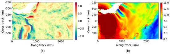
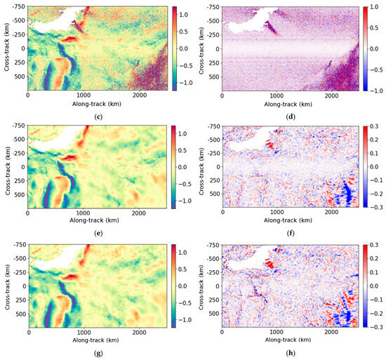
Figure 4.
Example of the ur fore (cycle 35, pass 1) between 0 and 2500 km along-track, located in the Philippine Sea. (a) True data (m/s); (b) wind speed (m/s); (c) noisy data (m/s); (d) noise (high-SNR configuration) (m/s); (e) data denoised by the UNet (m/s); (f) error made by the UNet (m/s); (g) data denoised by the Adaptative Gaussian Smoother (m/s); (h) error made by the Adaptative Gaussian Smoother (m/s).
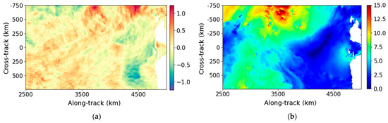
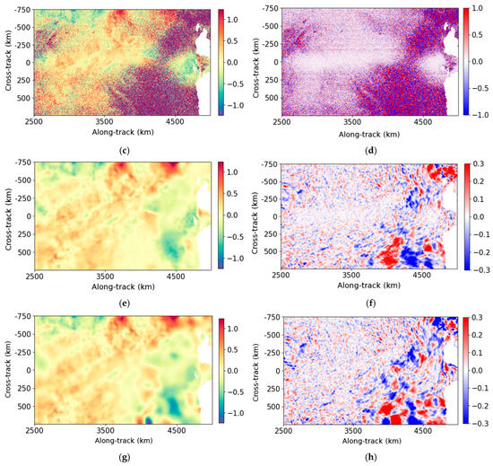
Figure 5.
Same example as Figure 4 but between 2500 and 5000 km along-track. (a) True data (m/s); (b) wind speed (m/s); (c) noisy data (m/s); (d) noise (high-SNR configuration) (m/s); (e) data denoised by the UNet (m/s); (f) error made by the UNet (m/s); (g) data denoised by the Adaptative Gaussian Smoother (m/s); (h) error made by the Adaptative Gaussian Smoother (m/s).
For wind speeds less than 5 m/s, oceanic structures are dominated by random noise which exceeds 1 m/s. For stronger winds, the noise is less important, and the oceanic structures are visible in the noisy field. The objective of denoising is to restore radial velocities, ideally for all wind speeds, and to reduce the error budget on ODYSEA measurements. In practice, low-wind regions have so much random noise that the objective is to retrieve as much SNR as possible in order to obtain higher spatial coverage for future scientific applications.
The main structures and amplitudes of the radial velocities are well recovered by both methods. For low winds, the UNet outperforms the Adaptive Gaussian Smoother. In fact, the Adaptive Gaussian Smoother generates more artificial oceanic content than the UNet. This is clearly visible, for instance, in Figure 5g, around 4000 km along-track, where some small eddy-like structures are created by the Adaptive Gaussian Smoother, whereas the UNet tends to smooth the signal. In these low-wind areas, the errors made by both methods can be higher than 30 cm/s. For winds greater than 5 m/s, the UNet restores smaller scales than the Adaptive Gaussian Smoother close to the nadir. This is illustrated in Figure 4 around 250 km along-track and 0 km cross-track. Far from the nadir, the denoising methods are comparable and the error is around 10 cm/s. The results of ur fore are similar to those of ur aft. Afterwards, the two components cannot be distinguished because they behave similarly with respect to denoising, since there is no azimuthal asymmetry in the current or wind features.
5.2. Statistics: Geographical and Temporal Variations
This part provides a quantitative analysis thanks to global, geographical and temporal scores.
Considering all measurements in any wind condition, the RMSE before denoising is very high (>200 cm/s). The noise-reduction algorithms reduce the RMSE to 11 cm/s (i.e., a reduction by a factor of 18) for the Adaptive Gaussian Smoother and to 7.6 cm/s (i.e., a reduction by a factor of 26) for the UNet (Table 3). However, these scores are largely dominated by the low winds. The ODYSEA mission requires the RMSE to be below 50 cm/s only for medium and strong wind speeds. This requirement is met before denoising. Indeed, for winds between 5 and 10 m/s (resp. winds greater than 10 m/s), the error before denoising is 47 cm/s (resp. 27 cm/s). However, denoising reduces this error by a factor of 6 (resp. 4) for the Adaptive Gaussian Smoother and by a factor of 7 (resp. 5) for the UNet. Thus, denoising can enhance the performance of the mission.
Table 3.
RMSE (cm/s) before and after denoising and noise reduction calculated for cycle 35. The scores are calculated globally and for three categories of winds.
For low wind speeds, the error before denoising exceeds 3.5 m/s. Both denoising methods significantly reduce this error: by a factor of 20 for the Adaptive Gaussian Smoother and by a factor of 33 for the neural network. The RMSE of the Adaptive Gaussian Smoother is 17 cm/s while for the UNet it is 10.6 cm/s. Therefore, these values can improve the coverage of the mission. The UNet outperforms the Adaptive Gaussian Smoother at all wind speeds.
The mean of the residuals is also calculated. Whatever the method and the wind speed, it is less than 1 mm/s. So, we can conclude that there is no bias introduced by the two methods.
Figure 6 shows maps of RMSE for the two denoising methods and a comparison between them. In the two methods, the geographical position of the ODYSEA swaths to be denoised is not provided as an input. The importance of RMSE in some areas is due to several factors. The most obvious are low-wind conditions. In these conditions, only the largest structures are restored. This can be seen in Figure 5 between 3500 and 5000 km along-track. In areas of high variability, such as the Gulf Stream or the Agulhas Current, both methods consider the smallest eddies as noise. The RMSE improvement for the UNet compared to the Gaussian filter is homogeneous and is around 25%, except in the polar areas.
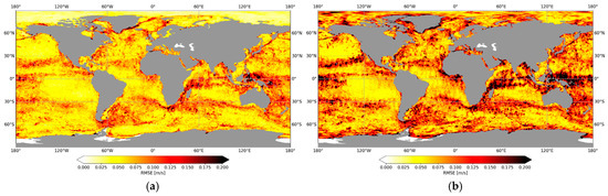
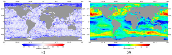
Figure 6.
RMSE of the UNet (a) and of the Adaptive Gaussian Smoother (b) computed for cycle 35. A comparison between the two methods is shown in (c). The blue corresponds to a better performance of the UNet, the red to a better performance of the Adaptive Gaussian Smoother. The associated wind speed average over cycle 35 is shown in (d).
Tracks are visible on the RMSE map of the Adaptive Gaussian Smoother (Figure 6b). This is due to the Smoother not being cross-track dependent, while the noise is. The UNet does not exhibit this artefact and is able to adapt denoising according to the distance from the nadir.
The results shown in Table 3 and Figure 6 were calculated for cycle 35 only, which was in December. Figure 7 shows the RMSE of the Adaptive Gaussian Smoother and the UNet for the whole period available, i.e., from February 2020 to January 2021. The two hemispheres are separated in order to highlight any seasonal variations. The grey area corresponds to the training period.
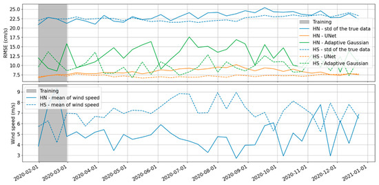
Figure 7.
(Top): RMSE of UNet denoising (orange) and the Adaptive Gaussian Smoother (green) as functions of time for the northern and southern hemispheres (HN and HS, respectively). By comparison, the standard deviation (std) of the ground truth is plotted in blue. The grey area corresponds to the training period. (Bottom): Mean of wind speeds as a function of time for the HN and HS. The RMSE, std and mean are computed over one cycle.
The performance of the UNet is similar during the training period and during the inference period. This means that the neural network is not overfitted. For the southern hemisphere, the RMSE is constant regardless of the season. For the northern hemisphere, the RMSE is slightly higher in summer (about 10 cm/s instead of 7.5 cm/s). This is due to a very low wind speed (<4 m/s in average) and in the training, the mean wind speed is between 4 and 9 m/s in both hemispheres. To improve the performance of the neural network, a training period of one month in winter and one month in summer should be used for each hemisphere. This would provide a good representation of all windy and oceanic conditions. The RMSE of the Adaptive Gaussian Smoother is higher than the one of the UNet whatever the season and the hemisphere.
Figure 7 also shows that the error made by the UNet is 2.5 to 3 times lower than the variability of the true radial velocities at the scale of MITgcm intrinsic resolution.
5.3. Spectral Analysis
Figure 8 shows Power Spectral Density (PSD) computed on noisy, true and denoised radial velocities under different wind conditions. The ratio between the PSD of the error and the one for ground truth allows the determination of the resolved scale given by SNR = 1. An SNR = 1 indicates where the error and/or the noise dominates the oceanic current modulation.
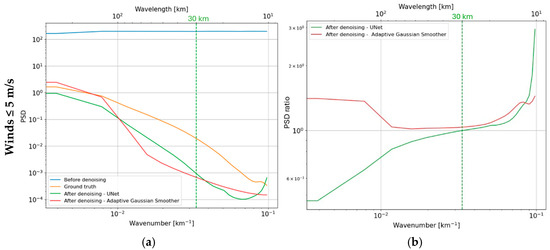
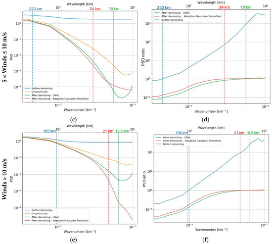
Figure 8.
Spectral analysis of the radial velocities before denoising (blue), after the UNet (green), after the Adaptive Gaussian Smoother (red) and of the true radial velocities (orange) in different wind conditions. The PSD (left column (a,c,e)) is computed from the average of each along-track PSD. The right column (b,d,f) shows the spectrum of the error over the spectrum of the ground truth. The dashed lines indicate the wavelength at which the noise dominates the signal. On (b), the PSD ratio before denoising is out of range and the PSD ratio of the Adaptive Gaussian Smoother never crosses the value 1, meaning that the wavelength at which the noise dominates is higher than 500 km.
For winds lower than 5 m/s (Figure 8a,b), the noise dominates the oceanic signal at wavelengths between 10 and 500 km. No structures can be observed below 500 km wavelength. Hence, the resolved scale is higher than 500 km. The PSD of the data denoised by the Adaptive Gaussian Smoother is more energetic than the ground truth at long wavelengths and is less energetic below 100 km wavelength. The associated resolved scale is higher than 500 km, meaning that no structures are correctly recovered. For UNet, the spectrum is less energetic at all wavelengths. Denoising the radial velocities using a neural network gives the best results for low winds: structures up to 30 km wavelength are correctly reconstructed.
For moderate (i.e., winds between 5 and 10 m/s, Figure 8c,d) and strong winds (i.e., winds greater than 10 m/s, Figure 8e,f), the noise dominates the oceanic content below 200 and 100 km wavelengths, respectively. Both methods can reduce this resolved scale. For the Adaptive Gaussian Smoother, the resolved scale is 34 km for moderate winds and 21 km for strong winds. For the UNet, more structures are better recovered. Thus, its resolved scale is 18 km for moderate winds and 15.5 km for strong winds. Regardless of the noise-reduction algorithms used, the spectrums are less energetic than the ground truth at short wavelengths.
5.4. Impact of Denoising on Velocities and Relative Vorticity
Radial velocities are not directly interpretable physical variables. Indeed, the scientific community will mainly use the horizontal velocity (U, V components) which is reconstructed from fore and aft radial velocities. This part presents the impact of denoising on U, V components. Figure 9 and Figure 10 present the U, V components derived from the radial velocities denoised by the UNet (Figure 4 and Figure A5). A comparison with the ground truth is also shown. The same example of the velocity denoised by the Adaptive Gaussian Smoother is presented in Appendix D. The error is most significant near the nadir; an error of a few mm/s in the radial velocity causes an error of a few cm/s in U, V. This is caused by the geometry of the problem; the two vectors of ur are quasi-colinear near the nadir (Figure 1). Data close to the swath borders are also affected for the same reason. This is confirmed by Figure 11. The project suggests keeping data between 0.1 and 0.9 from the nadir (normalized distance), which means that 20% of the data is lost. The error made by denoising between 0.05 and 0.1 from the nadir and between 0.9 and 0.98 is the same order of magnitude as the error between 0.1 and 0.9. So, with denoising, keeping data between 0.05 and 0.98 can be considered and only 7% of the data would be lost. In this case, the RMSE values are still satisfactory; less than 16 cm/s near the nadir and close to the swath borders. Elsewhere, the error is lower than 10 cm/s for areas affected by medium and strong wind conditions (Figure 9e,f). As for the radial velocities, the error ranges from 10 to 30 cm/s in areas with low winds (Figure 10e,f). Please note that the RMSE differs for the two components of the velocity due to the reconstruction method and to the geometry of the measurement.
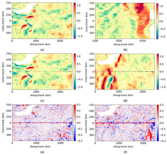
Figure 9.
Example of the velocity components (U and V) between 0 and 2500 km along-track. The velocity computed after the UNet is derived from the radial velocities shown in Figure 4 and Figure A5. (a) True U (m/s); (b) true V (m/s); (c) U derived from the UNet (m/s); (d) V derived from the UNet (m/s); (e) U error of the UNet (m/s); (f) V error of the UNet (m/s).
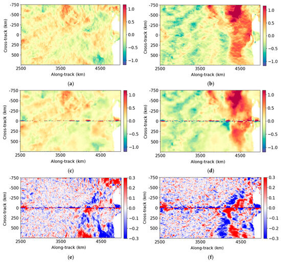
Figure 10.
Example of the velocity components (U and V) between 2500 and 5000 km along-track. The velocity computed after the UNet is derived from the radial velocities shown in Figure 5 and Figure A6. (a) True U (m/s); (b) true V (m/s); (c) U derived from the UNet (m/s); (d) V derived from the UNet (m/s); (e) U error of the UNet (m/s); (f) V error of the UNet (m/s).
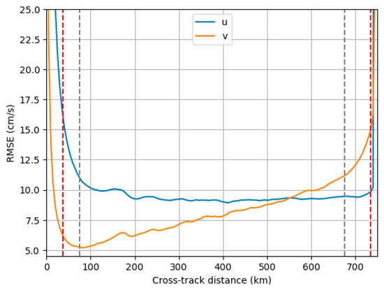
Figure 11.
RMSE of the U, V components as a function of the cross-track distance. The grey lines correspond to the distances 0.1 and 0.9 from the nadir (normalized distance) and the red lines correspond to the distances 0.05 and 0.98 from the nadir. It is calculated for all wind speeds.
Several quantities can be derived from the velocity, such as relative vorticity, divergence and strain rate. These quantities allow us to understand the interaction between wind and ocean [20], the oceanic turbulence [21], the vertical fluxes in the ocean [22]. In this study, we focus only on relative vorticity. The noise in the velocity field is amplified by the derivatives as shown in Figure 12b and Figure 13b. No structures can be exploited at 5 km resolution, a resolution out of the scope of ODYSEA science objectives. The relative vorticity derived from the field denoised by the UNet allows the main fronts and eddies to be reconstructed (Figure 12 and Figure 13). The RMSE of the relative vorticity is shown in Table 4. Globally, the RMSE is reduced by a factor of 100 after denoising. Following the same behavior as radial velocities, low winds dominate the RMSE. In this case, the RMSE of the relative vorticity is drastically reduced: 35 before denoising and 0.3 after applying the neural network. For medium and strong winds, the RMSE is divided by 26 and 14, respectively.
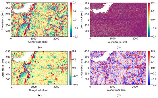
Figure 12.
Example of relative vorticity between 0 and 2500 km along-track. The relative vorticity computed after the UNet is derived from velocities shown in Figure 9. (a) True relative vorticity (−); (b) noisy relative vorticity (−); (c) relative vorticity derived from the UNet (−); (d) error of relative vorticity of the UNet (−).
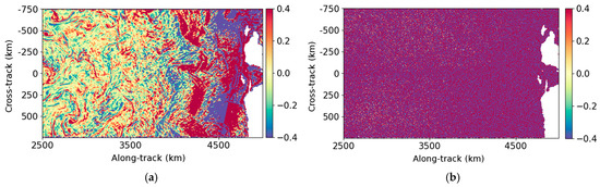
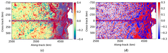
Figure 13.
Example of relative vorticity between 2500 and 5000 km along-track. The relative vorticity computed after the UNet is derived from velocities shown in Figure 10. (a) True relative vorticity (−); (b) noisy relative vorticity (−); (c) relative vorticity derived from the UNet (−); (d) error of relative vorticity of the UNet (−).
Table 4.
RMSE of the relative vorticity before and after denoising calculated for cycle 35. The RMSE is calculated globally except between 6°N and 6°S.
The relative vorticity derived from radial velocities denoised by the Adaptive Gaussian Smoother is shown in Appendix D. Discontinuities are visible, and the main eddies are not as well restored as with the UNet.
6. Robustness of the Model
6.1. Method Applied to Test the Robustness of the UNet
In this section, the robustness and the stability of the neural network will be tested. The Adaptive Gaussian Smoother is not used and should be readjusted for each new dataset. The objective of this section is to test the UNet on new data that the network has never seen before. To do this, the following method is applied:
- Change one characteristic of the dataset compared with the training dataset. This can be either a different noise or a different ocean model. Simulated data is not an exact representation of reality. The noise level impacting the real ODYSEA data may be stronger or weaker, the noise may be correlated or uncorrelated, impacted by residuals from previous processing, etc. This is exactly the case with SWOT, where the real noise is correlated and weaker than in the simulations [10]. Moreover, the ocean model is only an imperfect representation of the real ocean.
- Application of the UNet on radial velocities on this new dataset in inference without re-training. As a reminder, the UNet was trained and tested on the high-SNR configuration and on the MITgcm. Applying it without re-training will allow us to see how the UNet behaves when faced with new data, and also to determine whether or not it is overfitted.
- Performance evaluation in the same way as in the previous section. The results presented previously will be used as a baseline.
6.2. Scenario: Change of the Noise Configuration
The project proposes several noise configurations. The objective of this scenario is to evaluate the robustness of the UNet on another noise level by changing the noise configuration. For low winds, the low-SNR configuration (see Table 1) is noisier than the high-SNR configuration for the training (Figure 14); the RMSE before denoising is higher than 5 m/s for low winds (Table 5). For medium and strong winds, the data is less noisy than for the high-SNR configuration. This new noise configuration allows us to have more extreme values and to evaluate the behavior of the UNet with them. The inference was carried out in December in order to be comparable with previous results. The results obtained are presented in Table 5.
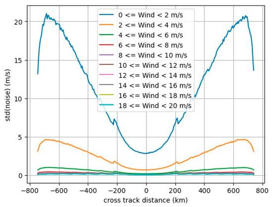
Figure 14.
Noise as function of cross-track distance and windspeed for the low-SNR configuration.
Table 5.
RMSE (cm/s) before and after denoising by the UNet and the noise reduction for the different scenarios. The RMSE is calculated for the entire available domain and for three categories of winds.
This scenario provided a satisfactory performance. For low wind speeds, the RMSE after denoising is around 11 cm/s which corresponds to dividing the error by 44. Even if the noise level is 1.5 times higher than in the training dataset before denoising, the error made by the neural network increases by only 5%. The resolved scale is 39 km, i.e., a degradation of 9 km compared to the baseline.
For all wind speeds greater than 5 m/s, the RMSE after denoising is between 4.5 and 5.5 cm/s, i.e., a noise reduction between 4 and 6. If the noise level is lower than expected, the error made by the UNet is also lower than the baseline. The resolved scale is similar to the baseline, which is between 15 and 20 km. Therefore, the UNet is robust to different noise levels.
6.3. Scenario: Change of the Ocean Model
In this second scenario, the simulated ODYSEA swaths are based on the Coastal and Regional Ocean Community model (CROCO) [23,24] instead of the MITgcm. The simulation is forced at the boundaries by the Mercator Glorys12V1 product [25] and by barotropic tides from the global tidal model TPXOv.7 [26]. Its domain is more restrictive than the domain of the MITgcm; it only extends from 22.5° to 48.84°N and from 36° to 82°W, which corresponds to the Gulf Stream. CROCO has a higher spatial resolution (approximately 2 km) so smaller oceanic structures are resolved. Contreras et al. [27,28] showed that this model is generally in good agreement with the observations and reproduces the dynamics of the Gulf Stream well. Further information on this version of CROCO is available in [27,28]. Level 2-simulated ODYSEA data are available from January 2005 to March 2005. The entire dataset is used for the inference. The noise configuration used in this case is the high-SNR configuration.
Table 5 summarizes the scores for this scenario. For low-wind speed conditions, the RMSE after denoising is approximately 13 cm/s. While this value is superior to the baseline, this performance is still satisfying. This slight degradation is due to two main points. Firstly, the RMSE for this scenario is calculated over the CROCO domain, while the RMSE of the baseline is computed globally. The second point is that the oceanic features differ slightly between the CROCO ocean model and the ocean model learnt by the UNet. Consequently, the neural network tries to recreate MITgcm-like structures. However, the UNet is able to restore oceanic structures down to 25 km. For medium and strong winds, the RMSEs are also slightly above the baseline, but they are still acceptable.
7. Conclusions and Perspectives
The ODYSEA mission will make it possible for the first time to measure wind and current fields simultaneously. These fields will be affected by random measurement errors which increase very rapidly as wind speeds get lower. In very low wind conditions, the SNR is so bad that ODYSEA measurements become barely usable (lost coverage). Even if the requirements are met despite this noise, it is better to have the lowest possible noise level for future scientific applications. In this context, the objective of this study was to evaluate the benefits of a denoising algorithm in various wind conditions.
To achieve this goal, the UNet developed for the SWOT data [8] was adapted to ODYSEA raw variables and trained to meet enhanced performances and enhanced coverage of future ODYSEA products. An Adaptive Gaussian Smoother which is wind-dependent was also developed in order to compare the results to a classical spatial filtering approach. Simulated ODYSEA swaths are used and a comparison to the ground truth is thus possible. The results show the necessity of noise reduction for users who want to use data impacted by low wind speeds and derived fields. The two methods significantly reduce random noise. But both methods exhibit some smoothing (not just denoising) properties, although the Gaussian kernel becomes an increasingly aggressive smoother in low wind conditions, whereas the UNet performs in a somewhat more robust way in all wind conditions. In low wind conditions, the error before denoising is more than 3 m/s and after applying the neural network, the error is only 11 cm/s. The ocean structures are correctly restored up to 30 km wavelengths. Even though the error is lower under medium and strong wind conditions, we should not neglect it. In fact, after calculating derivatives such as relative vorticity at 5 km sampling, a low noise level is amplified and can create major discontinuities. In summary, the UNet performs better than the Adaptive Gaussian Smoother. The UNet is also relatively stable over time and spatially homogeneous. The robustness of the model for other noise configurations and an ocean model was tested. In both cases, the UNet performed similarly to the dataset on which it was trained.
The work on the SWOT denoising has highlighted that similarity between training and inference dataset is crucial [10]. Indeed, the performances are degraded when the neural network is applied on real data that does not look like simulated data. These differences between the real dataset and the simulated dataset are due to two main factors. The first one is that the real ocean differs from the simulations used in the training dataset. The internal waves and solitons are not resolved in the simulated dataset, such as the geophysical errors due to the atmosphere or the waves. The second main difference is that there are still uncertainties about the level of noise that will be present in the data. In this study and in the dataset available on Aviso, only the wind speed influences the noise level and not the wind direction. The robustness of the UNet to correlated noise has also not been tested.
Moreover, the performance of the two methods of denoising is sub-optimal and can be improved between now and the launch. Firstly, other input variables of both methods can be added, such as ocean variability or cross-track distance. The training of UNet can also be carried out on data from both hemispheres in winter and in summer in order to learn to handle all oceanic conditions and to be more robust. Furthermore, rather than predicting only denoised radial velocity, the neural network could also provide derivatives of velocity (e.g., vorticity) in order to not be dependent on the derivation method. Finally, the UNet has a simple architecture, and it could be complexified. Indeed, more complex UNets have recently been developed [29,30,31] and demonstrate good performance. Moreover, the field of neural networks is constantly evolving; better architectures will be developed before the launch and could be applied to ODYSEA data. All these suggestions for improvement could be implemented when a more realistic simulation is available.
Author Contributions
Conceptualization and methodology, A.T. and C.A.; software, A.T.; input data and analysis, A.T., L.G. and C.A.; writing, A.T., R.B. and C.U.; supervision, M.-I.P., R.B. and G.D. All authors have read and agreed to the published version of the manuscript.
Funding
This research was financially and technically supported by the French Space Agency (CNES) (Grant number: 240844).
Data Availability Statement
The raw data supporting the conclusions of this article will be made available by the authors on request.
Acknowledgments
The authors would like to thank all the people involved, including the members of ODYSEA project.
Conflicts of Interest
Authors Anaëlle Tréboutte, Cécile Anadon, Marie-Isabelle Pujol was employed by the company Collecte Localisation Satellites (CLS). Author Clément Ubelmann was employed by the company Datlas. The remaining authors declare that the research was conducted in the absence of any commercial or financial relationships that could be construed as a potential conflict of interest.
Appendix A. Impact of the Input Dataset in the UNet Training
First, this appendix shows the impact of the normalization of the ODYSEA samples during the training. In many neural network trainings, it is recommended to normalize the data to be between –1 and 1. However, in the ODYSEA problem, the radial velocity is already centered by definition. If normalization is applied, the standard deviation and mean of the noisy field are used, as this is the only field available if UNet is applied to real data. The noise level drives the standard deviation, which is up to 50 times higher than the ground truth standard deviation (Figure A1). This results in ocean structures of lower intensity and sometimes very close to 0. The mean is also slightly modified by the presence of noise (up to 3 cm/s) (Figure A1). The consequence is that a small denoising error is amplified and a bias is created when applying normalization (Figure A2).

Figure A1.
Differences in means between noisy field and ground truth (left) and ratio of standard deviation (right) for each sample (6400 km along-track and 1500 km across-track).

Figure A2.
Mean of residuals after training the UNet with normalized radial velocities (left) and with raw radial velocities (right).
During the tuning phase of the UNet, several configurations of input variables were tested in order to have the best denoising effects:
- ur aft and ur fore separately (hereafter called conf 1);
- ur aft and ur fore jointly (conf 2);
- ur aft and ur fore jointly and the true wind speed (conf 3).
As described in the previous paragraph, the radial velocities are not normalized while the wind speed is divided by the maximal values of wind speed to have a field between 0 and 1.
Table A1 summarizes the RMSEs for the three configurations and for the different categories of wind speed. Using the two components of the radial velocities helps the neural network to understand the geometric relationship between the two components of the radial velocity (Figure 1). Taking the wind speed does not significantly improve the results (differences lower than 1 mm/s) and it does not add useful information for denoising. Therefore, only the combination of the two components of the radial velocities is used for this study.
Table A1.
RMSE (cm/s) before and after denoising calculated for cycle 35 for 3 configurations of input variables. The RMSE is calculated globally and for three categories of winds. Conf 1: ur aft and ur fore separately, Conf 2: ur aft and ur fore jointly and Conf 3: ur aft and ur fore jointly and the true wind speed.
| Global | Winds ≤ 5 m/s | 5 < Winds ≤ 10 m/s | Winds > 10 m/s | |
|---|---|---|---|---|
| Before denoising | >200 | >350 | 47 | 27 |
| Conf 1 | 7.8 | 10.8 | 6.2 | 5.3 |
| Conf 2 | 7.6 | 10.6 | 6.0 | 5.2 |
| Conf 3 | 7.6 | 10.6 | 6.0 | 5.2 |
Appendix B. Impact of the Derivation Method
Several methods are available for computing derivatives such as the simple centered scheme or stencil derivative. In this study, the 9-point stencil derivative is used with the following formula (currently used in the literature):
where N is the pixel to derive.
f′(N) = 0.00357143 × f(N − 4) −0.03809524 × f(N − 3) + 0.2 × f(N − 2), −0.8 × f(N − 1) + 0.8 × f(N + 1) − 0.2 × f(N +
2) + 0.03809524 × f(N + 3) − 0.00357143 × f(N)
2) + 0.03809524 × f(N + 3) − 0.00357143 × f(N)
The effect of this stencil derivative is to minimize the errors from the discretization once the fields have been produced by the denoiser. One possibility is indeed to include the derivation process in the denoiser, therefore avoiding the use of an explicit numerical scheme. However, for simplicity, a two-step process (denoising then stencil derivation) is used. As the impact would be small for this problem, given that the grid size is sufficiently small, w.r.t. is the shortest wavelength resolved in the vorticity field (derivative of the velocity).
A simple test as carried out to assess the sensitivity of the derivation method as a function of wavelength. A random signal following a red spectral slope is generated (Figure A3). The signal is discretized and the derivatives are computed with a simple centered scheme, a 5-point stencil derivative and a 9-point stencil derivative. The spectra of the different signals over a large number (10,000) of realizations is represented in Figure A4.

Figure A3.
Illustration of a true continuous signal (gray) sampled every 5 km (dots), and its derivatives from the continuous truth (black) and from various discretized schemes (green, blue and red).

Figure A4.
Power spectral densities of the derivatives (continuous in black, green, blue and red for the different discretized schemes. The thin curves represent the PSD of the residual errors for the different schemes).
From these results, the stencil provides a significant improvement between a 10 km wavelength and a 50 km wavelength. The improvement comes from resolving more energy (red curve closer to the black) and with fewer residual errors (thin red curve below the green curve). However, beyond a 50 km wavelength, the discretization errors become extremely small anyway. Therefore, for the useful signal we are resolving for the vorticity (mostly beyond 50 km as suggested by Figure 12c and Figure 13c) we believe the impact of the derivation method is not significant.
Appendix C. Denoising of Ur Aft
The following figures show the denoising of the ur aft component by the UNet and by the Adaptive Gaussian Smoother. Figure A5 (resp. Figure A6) presents a radial velocity field with a low level of noise (resp. high level of noise). The denoising of the same examples but for the ur fore component is shown on Figure 4 and Figure 5.

Figure A5.
Example of the ur aft component (cycle 35, pass 1) between 0 and 2500 km along-track in the Philippine Sea. (a) True data (m/s); (b) wind speed (m/s); (c) noisy data (m/s); (d) noise (high-SNR configuration) (m/s); (e) data denoised by the UNet (m/s); (f) error made by the UNet (m/s); (g) data denoised by the Adaptative Gaussian Smoother (m/s); (h) error made by the Adaptative Gaussian Smoother (m/s).

Figure A6.
Same example as Figure A5 but between 2500 and 5000 km along-track. (a) True data (m/s); (b) wind speed (m/s); (c) noisy data (m/s); (d) noise (high-SNR configuration) (m/s); (e) data denoised by the UNet (m/s); (f) error made by the UNet (m/s); (g) data denoised by the Adaptative Gaussian Smoother (m/s); (h) error made by the Adaptative Gaussian Smoother (m/s).
Appendix D. Velocities and Relative Vorticities Deduced from the Adaptive Gaussian Smoother
This appendix illustrates two examples of the velocity components (Figure A7 and Figure A8) and the relative vorticity (Figure A9 and Figure A10). They are deduced from the radial velocities denoised by the Adaptive Gaussian Smoother. A comparison to the ground truth is also presented.

Figure A7.
Example of the velocity components (U and V) between 0 and 2500 km along-track. The velocity computed after the Adaptive Gaussian Smoother’s effect is deduced from the radial velocities is shown in Figure 4 and Figure A5. (a) True U (m/s); (b) true V (m/s); (c) U derived from the UNet (m/s); (d) V derived from the UNet (m/s); (e) U error of the Adaptive Gaussian Smoother (m/s); (f) V error of the Adaptive Gaussian Smoother (m/s).


Figure A8.
Example of the velocity components (U and V) between 2500 and 5000 km along-track. The velocity computed after the Adaptive Gaussian Smoother effect is deduced from the radial velocities is shown in Figure 5 and Figure A6. (a) True U (m/s); (b) true V (m/s); (c) U deduced from the Adaptive Gaussian Smoother (m/s); (d) V deduced from the Adaptive Gaussian Smoother (m/s); (e) U error of the Adaptive Gaussian Smoother (m/s); (f) V error of the Adaptive Gaussian Smoother (m/s).


Figure A9.
Example of the relative vorticity between 0 and 2500 km along-track. The relative vorticity computed after the Adaptive Gaussian Smoother is deduced from velocities shown in Figure A7. (a) True relative vorticity (−); (b) noisy relative vorticity (−); (c) relative vorticity deduced from the Adaptive Gaussian Smoother (−); (d) error of relative vorticity of the Adaptive Gaussian Smoother (−).

Figure A10.
Example of the relative vorticity between 2500 and 5000 km along-track. The relative computed vorticity after the Adaptive Gaussian Smoother is deduced from the velocities is shown in Figure A8. (a) True relative vorticity (−); (b) noisy relative vorticity (−); (c) relative vorticity deduced from the Adaptive Gaussian Smoother (−); (d) error of relative vorticity of the Adaptive Gaussian Smoother (−).
References
- Ferrari, R.; Wunsch, C. Ocean Circulation Kinetic Energy: Reservoirs, Sources, and Sinks. Annu. Rev. Fluid Mech. 2009, 41, 253–282. [Google Scholar] [CrossRef]
- Rodríguez, E.; Wineteer, A.; Perkovic-Martin, D.; Gál, T.; Stiles, B.W.; Niamsuwan, N.; Rodriguez Monje, R. Estimating Ocean Vector Winds and Currents Using a Ka-Band Pencil-Beam Doppler Scatterometer. Remote Sens. 2018, 10, 576. [Google Scholar] [CrossRef]
- Rodríguez, E.; Bourassa, M.; Chelton, D.; Farrar, J.T.; Long, D.; Perkovic-Martin, D.; Samelson, R. The Winds and Currents Mission Concept. Front. Mar. Sci. 2019, 6, 438. [Google Scholar] [CrossRef]
- Frasier, S.J.; Camps, A.J. Dual-beam interferometry for ocean surface current vector mapping. IEEE Trans. Geosci. Remote Sens. 2001, 39, 401–414. [Google Scholar] [CrossRef]
- Gaultier, L. Technical Note: ODYSEA L2 Simulated Datasets. 2024. Available online: https://www.aviso.altimetry.fr/fileadmin/documents/data/tools/hdbk_Odysea_simulator_v1.pdf (accessed on 26 October 2025).
- Wineteer, A.; Torres, H.S.; Rodriguez, E. On the Surface Current Measurement Capabilities of Spaceborne Doppler Scatterometry. Geophys. Res. Lett. 2020, 47, e2020GL090116. [Google Scholar] [CrossRef]
- Gómez-Navarro, L.; Cosme, E.; Sommer, J.; Papadakis, N.; Pascual, A. Development of an Image De-Noising Method in Preparation for the Surface Water and Ocean Topography Satellite Mission. Remote Sens. 2020, 12, 734. [Google Scholar] [CrossRef]
- Tréboutte, A.; Carli, E.; Ballarotta, M.; Carpentier, B.; Faugère, Y.; Dibarboure, G. KaRIn Noise Reduction Using a Convolutional Neural Network for the SWOT Ocean Products. Remote Sens. 2023, 15, 2183. [Google Scholar] [CrossRef]
- Fu, L.-L.; Pavelsky, T.; Cretaux, J.-F.; Morrow, R.; Farrar, J.T.; Vaze, P.; Sengenes, P.; Vinogradova-Shiffer, N.; Sylvestre-Baron, A.; Picot, N.; et al. The Surface Water and Ocean Topography Mission: A Breakthrough in Radar Remote Sensing of the Ocean and Land Surface Water. Geophys. Res. Lett. 2024, 51, e2023GL107652. [Google Scholar] [CrossRef]
- Dibarboure, G.; Anadon, C.; Briol, F.; Cadier, E.; Chevrier, R.; Delepoulle, A.; Faugère, Y.; Laloue, A.; Morrow, R.; Picot, N.; et al. Blending 2D topography images from SWOT into the altimeter constellation with the Level-3 multi-mission DUACS system. EGUsphere 2024, 2024, 1–64. [Google Scholar] [CrossRef]
- OceanDataLab. Level-2 ODYSEA Simulated Dataset. 2024. Available online: https://www.aviso.altimetry.fr/en/data/products/value-added-products/simulated-level-2-odysea-dataset.html (accessed on 26 October 2025).
- Komatsu, R.; Gonsalves, T. Comparing U-Net Based Models for Denoising Color Images. AI 2020, 1, 465–486. [Google Scholar] [CrossRef]
- Kovacs, A.; Bukki, T.; Legradi, G.; Meszaros, N.J.; Kovacs, G.Z.; Prajczer, P.; Tamaga, I.; Seress, Z.; Kiszler, G.; Forgacs, A.; et al. Robustness analysis of denoising neural networks for bone scintigraphy. Nucl. Instrum. Methods Phys. Res. Sect. Accel. Spectrometers Detect. Assoc. Equip. 2022, 1039, 167003. [Google Scholar] [CrossRef]
- Ronneberger, O.; Fischer, P.; Brox, T. U-Net: Convolutional Networks for Biomedical Image Segmentation. arXiv 2015, arXiv:1505.04597. [Google Scholar] [CrossRef]
- Agrawal, S.; Barrington, L.; Bromberg, C.; Burge, J.; Gazen, C.; Hickey, J. Machine Learning for Precipitation Nowcasting from Radar Images. arXiv 2019, arXiv:1912.12132. [Google Scholar] [CrossRef]
- Mirouze, I.; Rémy, E.; Lellouche, J.-M.; Martin, M.J.; Donlon, C.J. Impact of assimilating satellite surface velocity observations in the Mercator Ocean International analysis and forecasting global 1/4° system. Front. Mar. Sci. 2024, 11, 1376999. [Google Scholar] [CrossRef]
- Ubelmann, C.; Dibarboure, G.; Gaultier, L.; Ponte, A.; Ardhuin, F.; Ballarotta, M.; Faugère, Y. Reconstructing Ocean Surface Current Combining Altimetry and Future Spaceborne Doppler Data. J. Geophys. Res. Oceans 2021, 126, e2020JC016560. [Google Scholar] [CrossRef]
- Wang, J.; Fu, L.-L.; Torres, H.S.; Chen, S.; Qiu, B.; Menemenlis, D. On the Spatial Scales to be Resolved by the Surface Water and Ocean Topography Ka-Band Radar Interferometer. J. Atmospheric Ocean. Technol. 2019, 36, 87–99. [Google Scholar] [CrossRef]
- Arbic, B.K.; Scott, R.B.; Chelton, D.B.; Richman, J.G.; Shriver, J.F. Effects of stencil width on surface ocean geostrophic velocity and vorticity estimation from gridded satellite altimeter data. J. Geophys. Res. Oceans 2012, 117. [Google Scholar] [CrossRef]
- Seo, H.; Miller, A.J.; Norris, J.R. Eddy–Wind Interaction in the California Current System: Dynamics and Impacts. J. Phys. Oceanogr. 2016, 46, 439–459. [Google Scholar] [CrossRef]
- Torres, H.S.; Rodriguez, E.; Wineteer, A.; Klein, P.; Thompson, A.F.; Callies, J.; D’Asaro, E.; Perkovic-Martin, D.; Farrar, J.T.; Polverari, F.; et al. Airborne observations of fast-evolving ocean submesoscale turbulence. Commun. Earth Environ. 2024, 5, 771. [Google Scholar] [CrossRef]
- Carli, E.; Morrow, R.; Vergara, O.; Chevrier, R.; Renault, L. Ocean 2D eddy energy fluxes from small mesoscale processes with SWOT. Ocean Sci. 2023, 19, 1413–1435. [Google Scholar] [CrossRef]
- Debreu, L.; Marchesiello, P.; Penven, P.; Cambon, G. Two-way nesting in split-explicit ocean models: Algorithms, implementation and validation. Ocean Model. 2012, 49–50, 1–21. [Google Scholar] [CrossRef]
- Shchepetkin, A.F.; McWilliams, J.C. Quasi-Monotone Advection Schemes Based on Explicit Locally Adaptive Dissipation. Mon. Wea. Rev. 1998, 126, 1541–1580. [Google Scholar] [CrossRef]
- Lellouche, J.-M.; Greiner, E.; Le Galloudec, O.; Garric, G.; Regnier, C.; Drevillon, M.; Benkiran, M.; Testut, C.-E.; Bourdalle-Badie, R.; Gasparin, F.; et al. Recent updates to the Copernicus Marine Service global ocean monitoring and forecasting real-time 1∕12° high-resolution system. Ocean Sci. 2018, 14, 1093–1126. [Google Scholar] [CrossRef]
- Egbert, G.D.; Erofeeva, S.Y. Efficient Inverse Modeling of Barotropic Ocean Tides. J. Atmos. Oceanic Technol. 2002, 19, 183–204. [Google Scholar] [CrossRef]
- Contreras, M.; Renault, L.; Marchesiello, P. Understanding Energy Pathways in the Gulf Stream. J. Phys. Oceanogr. 2023, 53, 719–736. [Google Scholar] [CrossRef]
- Contreras, M.; Renault, L.; Marchesiello, P. Tidal Modulation of Energy Dissipation Routes in the Gulf Stream. Geophys. Res. Lett. 2023, 50, e2023GL104946. [Google Scholar] [CrossRef]
- Lu, Y.; Ying, Y.; Lin, C.; Wang, Y.; Jin, J.; Jiang, X.; Shuai, J.; Li, X.; Zhong, J. UNet-Att: A self-supervised denoising and recovery model for two-photon microscopic image. Complex Intell. Syst. 2024, 11, 55. [Google Scholar] [CrossRef]
- Zhang, K.; Li, Y.; Liang, J.; Cao, J.; Zhang, Y.; Tang, H.; Fan, D.-P.; Timofte, R.; Gool, L.V. Practical Blind Image Denoising via Swin-Conv-UNet and Data Synthesis. Mach. Intell. Res. 2023, 20, 822–836. [Google Scholar] [CrossRef]
- Jang, H.; Park, J.; Jung, D.; Lew, J.; Bae, H.; Yoon, S. PUCA: Patch-Unshuffle and Channel Attention for Enhanced Self-Supervised Image Denoising. arXiv 2023, arXiv:2310.10088. [Google Scholar] [CrossRef]
Disclaimer/Publisher’s Note: The statements, opinions and data contained in all publications are solely those of the individual author(s) and contributor(s) and not of MDPI and/or the editor(s). MDPI and/or the editor(s) disclaim responsibility for any injury to people or property resulting from any ideas, methods, instructions or products referred to in the content. |
© 2025 by the authors. Licensee MDPI, Basel, Switzerland. This article is an open access article distributed under the terms and conditions of the Creative Commons Attribution (CC BY) license (https://creativecommons.org/licenses/by/4.0/).