Geometric Error Analysis and Correction of Long-Term In-Orbit Measured Calibration Data of the LuTan-1 SAR Satellite

Highlights

What are the main findings?

• The planar positioning accuracy of the LuTan-1 SAR satellite over three years of in-orbit data meets the in-orbit testing requirements and remains stable.
• A full-chain geometric error analysis and correction method has been established, improving the positioning accuracy of corrected images to better than 3.0 m.

What are the implications of the main findings?

• The accuracy and stability of LuTan-1 SAR satellite data provide critical support for its applications in fields such as deformation monitoring.
• The full-chain geometric error analysis and correction method has laid the research foundation for enhancing the geometric quality and application services of domestic SAR satellites.

Abstract

LuTan-1 (LT-1) is China’s first L-band differential interferometric synthetic aperture radar system, comprising two multi-polarization SAR satellites, LT-1A and LT-1B. The satellite uses differential deformation measurement and interferometric altimetry technology to realize surface deformation monitoring and topographic mapping in designated areas. It has the characteristics of all-weather, all-time, and multi-polarization and can be applied to military and civilian fields. In order to further improve the accuracy of image geometric positioning, this paper analyzes the error sources of geometric positioning for the differential deformation measurement mode (strip 1) of the satellite service. The in-orbit data of three years since the launch (2022–2024) are selected to analyze the positioning accuracy and stability of the uncontrolled plane based on the corner reflector and active calibrator deployed in the calibration field. The experimental results show that the positioning accuracy of the satellite strip 1 image without a control plane meets the requirements of the in-orbit index and remains relatively stable. The geometric precision correction positioning accuracy after error source compensation is better than 3.0 m, providing a favorable support for the subsequent application.

1. Introduction

Synthetic aperture radar (SAR) [1,2,3] is an active microwave imaging device. Compared with optical images, SAR can generate high-resolution remote sensing images all day and in all weather conditions, playing an important role in military and civilian fields. LT-1 is an important part of the national medium- and long-term development plan for civil space infrastructure (2015–2025). It is the first L-band differential interferometric synthetic aperture radar system [4,5,6,7,8] launched by our country. The system consists of two satellites, A and B, which can work independently or cooperatively, as shown in Figure 1. Its imaging mode includes strip mode, scanning mode, and other experimental modes. The maximum resolution of strip mode is 3 m, and the maximum width is 250 km. The resolution of scan mode is 30 m, and the width is 400 km.

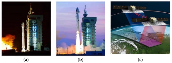
Figure 1. Launch and operation of the satellite: (a) LT-1A launch; (b) LT-1B launch; (c) schematic diagram of satellite operation.

The effective application of SAR requires high-precision geometric positioning of image pixels, especially in emergency monitoring tasks such as disaster monitoring and deformation monitoring. In recent years, with the rapid development of SAR satellites [9,10,11], the geometric positioning accuracy index has also been significantly improved. Launched by the European Space Agency in 1991, ERS-1 [12] was the world’s first SAR satellite to achieve high-precision geometric calibration. By utilizing control data from ground calibration sites, it calibrated key system parameters for uncontrolled positioning accuracy—specifically distance and azimuth corrections—enabling a single image to achieve geometric positioning accuracy of 13.18 m. Around 2007, Canada, Japan, Italy, and other countries successfully launched a number of high-resolution SAR satellites. For example, the ALOS-1 [13] launched by Japan employs ground-based calibration methods to geometrically calibrate its onboard SAR system, achieving a geometric positioning accuracy of 9.7 m in final strip mode images. The COSMO-SkyMed [14] launched by Italy utilizes four calibration sites within Italy and one overseas calibration site to perform geometric calibration and accuracy validation of its image products, achieving a geometric positioning accuracy of 3 m in strip mode and 1 m in spotlight mode. The Terra-SAR [15] satellite launched by Germany employs multiple point targets within a specific area constructed in southern Germany for geometric calibration. Following meticulous product processing, its geometric positioning accuracy can even reach the decimeter level. Although the research on geometric positioning accuracy in China started late, it has also made breakthrough progress. For example, the geometric positioning accuracy of the HJ-1C [16,17] satellite has increased from 136 m to 9 m. In 2017, the Institute of Electricity of the Chinese Academy of Sciences verified the geometric positioning accuracy of the GF-3 [18,19,20] satellite, which can reach about 3 m. High geometric positioning accuracy not only ensures a clear geometric correspondence between image pixels and actual geographical locations but also greatly facilitates the application of synthetic aperture radar images [21].

This paper conducts a comprehensive analysis of the geometric positioning error sources across the entire chain of the LT-1 satellite. Using corner reflectors and active calibrators deployed in the calibration field, it evaluates the geometric positioning accuracy and analyzes the stability of images acquired by the satellite during its three-year in-orbit operation. Finally, by compensating for the error sources, it achieves highly calibrated geometric positioning accuracy. Through large-scale data validation, the geometric positioning accuracy of the LT-1 satellite is significantly enhanced. This research not only establishes a foundation for addressing geometric quality in domestically produced SAR satellites but also provides long-term, stable data support for geological hazard monitoring in China. It serves as robust spatial technology support for applications including topographic surveying [22], deformation monitoring, resource exploration, disaster prevention and emergency response [23], and rapid military target positioning [24].

2. Error Source Analysis of Full-Link Geometric Positioning

In the process of Earth observation, satellites will be affected by various error sources, which will affect the geometric positioning accuracy of images. In order to achieve high-precision geometric positioning, it is necessary to understand the physical mechanism of these error sources and correct them accordingly. In this section, the sources of geometric positioning errors in LT-1 Earth observations are reviewed in detail, as shown in Figure 2, including antenna phase center error, control point positioning error, SAR payload error, atmospheric delay error, and imaging processing error.

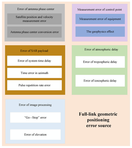
Figure 2. Error source of the full link.

2.1. Error of the Antenna Phase Center

The error of the antenna phase center mainly comes from the measurement error of satellite position and velocity [25] and the conversion error of the antenna phase center.

2.1.1. Satellite Position and Velocity Measurement Error

The satellite position error mainly refers to the three-axis error of a satellite along the tangent, normal, and radial directions. The tangent error will lead to azimuth positioning deviation of the target point; the normal error will lead to range positioning deviation of the target point; and the radial error will lead to inaccurate positioning of the target point in both range and azimuth. Satellite velocity errors are also errors in the above three-axis directions, which can lead to inaccurate Doppler calculations of the target, causing deviations in the imaging position and resulting in inaccurate geometric positioning.

At present, dual-frequency GPS orbit determination is used in the LT-1 satellite ground processing system. For Satellite A, the average differences in precise orbital position are 1.481 mm in the tangential direction, 1.433 mm in the normal direction, 1.330 mm in the radial direction, and 2.537 mm in the three-dimensional space. The average speed differences are 1.549 μm/s in the tangential direction, 1.715 μm/s in the normal direction, 1.533 μm/s in the radial direction, and 2.858 μm/s in the three-dimensional space. The mean values of the precise orbit position differences of Satellite B in the tangent, normal, radial, and three-dimensional directions are 1.129, 1.115, 1.155, and 1.996 mm, respectively. The mean values of the velocity differences in the tangent, normal, radial, and three-dimensional directions are 1.112, 1.122, 1.086, and 1.946 μm/s, respectively. In summary, the LT-1 satellite can determine millimeter-level precision orbits based on multi-frequency GNSS raw observation data. Figure 3 shows the 5 h a day overlapping position and velocity accuracy difference sequences of the precise orbits of LT-1A and LT-1B, respectively.

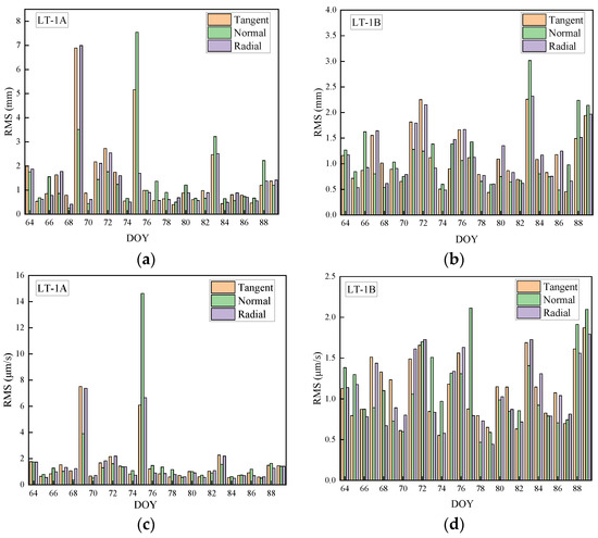
Figure 3. Satellite position and velocity accuracy difference sequence diagram: (a) LT-1A orbital position accuracy difference sequence; (b) LT-1B orbital position accuracy difference sequence; (c) LT-1A orbit velocity precision difference sequence; (d) LT-1B orbit velocity precision difference sequence.

2.1.2. Antenna Phase Center Conversion Error

Because the position of the satellite antenna phase center has a certain deviation from the position of the sensor measured by the satellite orbit, the position of the antenna phase center is used in the actual SAR imaging processing. Therefore, the satellite orbit measurements need to be converted to the position of the satellite antenna phase center; otherwise, it will cause geometric positioning deviation.

The LT-1 satellite employs a satellite coordinate system for converting coordinate position relationships during processing. It primarily utilizes six coordinate systems: the Earth-fixed coordinate system, the Earth-inertial coordinate system, the geocentric orbital coordinate system, the satellite orbital coordinate system, the satellite body coordinate system, and the satellite antenna coordinate system. Their representations are shown in Figure 4.

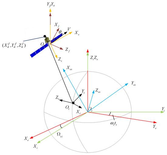
Figure 4. Representation in spatial geometric coordinate systems.

Geocentric coordinate system: As indicated by the red arrows in Figure 4, the origin is at the Earth’s center. The X-axis points toward the intersection of the Greenwich meridian and the equatorial plane. The Z-axis aligns with the Earth’s rotational axis, pointing toward the North Pole. The Y-axis is determined by the right-hand rule.

Earth-centered inertial coordinate system: As indicated by the green arrows in the figure, the origin is at the Earth’s center, the X-axis points toward the vernal equinoctial point, the Z-axis aligns with the Earth’s rotational axis toward the North Pole, and the Y-axis is determined by the right-hand rule. This coordinate system can be converted to the Earth-fixed coordinate system using the following transformation formula:

$$\left[\begin{array}{l}{X}_i\\ Y_i\\ Z_i\end{array}\right]=R_Z\left({\Omega }_{ei}\right)\left[\begin{array}{l}{X}_e\\ Y_e\\ Z_e\end{array}\right]$$

(1)

$$R_Z\left(\theta \right)=\left[\begin{array}{ccc}\cos \theta & \sin \theta & 0\\ -\sin \theta & \cos \theta & 0\\ 0& 0& 1\end{array}\right]$$

(2)

where $\theta >0$ denotes rotation along the positive direction of the coordinate axis, $\theta <0$ denotes rotation along the negative direction of the coordinate axis, $R_Z\left(\theta \right)$ represents the angle of rotation of the coordinate system around the Z-axis, and ${\mathsf{\Omega }}_{ei}$ represents the angle of rotation of the X-axis around the Z-axis in the Earth’s inertial coordinate system. When the satellite’s angle at perigee is ${\mathsf{\Omega }}_{ei0}$, then ${\mathsf{\Omega }}_{ei}$ is ${\mathsf{\Omega }}_{ei}={\mathsf{\Omega }}_{ei0}-{\omega }_{e}t,$ where ${\omega }_e$ is the angular velocity of the Earth’s rotation.

Geocentric orbital coordinate system: As indicated by the blue arrows in the figure, the origin is at the Earth’s center. The X-axis points toward the satellite, the Y-axis lies within the orbital plane and is perpendicular to the X-axis pointing in the satellite’s direction of motion, and the Z-axis is determined by the right-hand rule. The transformation relationship between this coordinate system and the geocentric orbital coordinate system is as follows:

$$R_X\left(\theta \right)=\left[\begin{array}{ccc}1& 0& 0\\ 0& \cos \theta & \sin \theta \\ 0& -\sin \theta & \cos \theta \end{array}\right]$$

(3)

$$\left[\begin{array}{l}{X}_{es}\\ Y_{es}\\ Z_{es}\end{array}\right]=R_Z\left(u\right)R_X\left(i\right)R_Z\left(\Omega \right)\left[\begin{array}{l}{X}_i\\ Y_i\\ Z_i\end{array}\right]$$

(4)

where $R_X\left(\theta \right)$ denotes the angle of rotation of the coordinate system about the X-axis, u is the satellite’s orbital azimuth angle, i is the satellite’s orbital inclination, and $\mathsf{\Omega }$ is the satellite’s ascending node right ascension.

Satellite orbital coordinate system: As indicated by the orange arrows in the figure, the origin is the satellite’s center of mass. The Z-axis points toward the Earth’s center, the X-axis lies within the orbital plane and points perpendicular to the Z-axis in the direction of motion, and the Y-axis is determined by the right-hand rule. The transformation from this coordinate system to the satellite orbital coordinate system is as follows:

$$\left[\begin{array}{l}{X}_s\\ Y_s\\ Z_s\end{array}\right]=R_X\left(-{\displaystyle \frac{\pi }{2}}\right)R_Z\left({\displaystyle \frac{\pi }{2}}\right)\left[\begin{array}{l}0\\ 0\\ R_S\end{array}\right]$$

(5)

where $R_s$ is the distance between the satellite’s instantaneous position and the center of the Earth.

Satellite body coordinate system: As indicated by the brown arrows in the figure, the origin is the satellite’s center of mass. When the satellite is in a stable orbital position, the axes of this coordinate system align with those of the satellite orbital coordinate system. The transformation from the satellite orbital coordinate system to this coordinate system is as follows:

$$R_Y\left(\theta \right)=\left[\begin{array}{ccc}\cos \theta & 0& -\sin \theta \\ 0& 1& 0\\ \sin \theta & 0& \cos \theta \end{array}\right]$$

(6)

$$\left[\begin{array}{l}{X}_f\\ Y_f\\ Z_f\end{array}\right]=R_X\left({\theta }_{roll}\right)R_Y\left({\theta }_{pitch}\right)R_Z\left({\theta }_{yaw}\right)\left[\begin{array}{l}{X}_s\\ Y_s\\ Z_s\end{array}\right]$$

(7)

where $R_Y\left(\theta \right)$ denotes the angle of rotation of the coordinate system about the Y-axis, while ${\theta }_{yaw}$, ${\theta }_{pitch},$ and ${\theta }_{roll}$ represent the yaw, pitch, and roll angles, respectively.

Satellite antenna coordinate system: As indicated by the gray arrows in the figure, the origin is the satellite’s center of mass. The X-axis points in the same direction as the X-axis in the satellite body coordinate system. The Z-axis points toward the beam center. The Y-axis is determined by the right-hand rule. The transformation from the satellite body coordinate system to this coordinate system is as follows:

$$\left[\begin{array}{l}{X}_a\\ Y_a\\ Z_a\end{array}\right]=\left[\begin{array}{ccc}1& 0& 0\\ 0& \cos {\theta }_L& -\sin {\theta }_L\\ 0& \sin {\theta }_L& \cos {\theta }_L\end{array}\right]\left[\begin{array}{l}{X}_f\\ Y_f\\ Z_f\end{array}\right]=R_X\left(-{\theta }_L\right)\left[\begin{array}{l}{X}_f\\ Y_f\\ Z_f\end{array}\right]$$

(8)

where ${\theta }_L$ denotes the antenna field of view in the satellite body coordinate system.

After performing the aforementioned transformation of the celestial coordinate system, the precise position of the antenna’s phase center can be obtained, with a conversion error of only decimeter magnitude.

2.2. Measurement Error of Control Points

In order to achieve high-precision geometric correction, ground control points are often needed. However, there are also some errors in the coordinate measurement of ground control points, which mainly come from two aspects. The first is the measurement error of the ground control point itself, and the second is the measurement error of the ground point coordinates caused by the geophysics effect.

2.2.1. Measurement Error

Ground control points are installed on fixed bases. The geodetic coordinates at the center of each base are measured according to the “Global Navigation Satellite System (GNSS) Surveying Specifications” with Class D point accuracy requirements (Table 1). During the measurement process of ground control points, measurement errors may occur due to environmental electromagnetic interference or other factors. Therefore, multiple measurements are taken for each ground control point coordinate, and the average value is used as the final result to ensure the accuracy of the control point coordinates.

Table 1. Accuracy requirements for each level.

Level	Point-to-Point Error		Mean Error in Baseline Components of Adjacent Points
	Horizontal Component	Vertical Component	Horizontal Component	Vertical Component
B	5 mm	10 mm	5 mm	10 mm
C	10 mm	15 mm	10 mm	20 mm
D	15 mm	30 mm	20 mm	40 mm
E	15 mm	30 mm	20 mm	40 mm

2.2.2. The Geophysics Effect

The geophysics effect is the second key factor in the measurement of GCPS. Usually, multiple corner reflectors and active calibrators are arranged as control points in the calibration field, and the reference coordinates of these control points are obtained, but these coordinates are based on the average earth surface as a reference; the real coordinates should be based on the satellite surface dynamic state at a certain observation epoch. Therefore, it is necessary to add the SAR observation target offset calculated by the dynamic model to the collected control point coordinates to establish the real control point position coordinates. The model includes all the effects of geophysical tides, such as solid tides, polar tides, ocean tides, and atmospheric loads, which cause the coordinates of control points to shift. The magnitudes of the effects are shown in Table 2, where the Earth’s solid tides, caused by the uplift of the Earth’s crust due to the gravitational attraction of the sun and moon, can be offset in the vertical direction by tens of centimeters. It produces an offset of about 5 cm in azimuth and is the most significant of all solid earth displacements.

Table 2. Amplitude of solid earth displacement effects.

Effect	Level/mm	Vertical/mm
Earth tide	±50.0	±200.0
Ocean tide	±10.0	±50.0
Pole shift	±1.5	±6.0
Tidal load of the atmosphere	±0.2	±1.5
Load of the ocean polar tide	±0.3	±0.5
Non-tidal load of the atmosphere	±3.0	±0.5
Long-term trends	Up to 100 mm/year	Up to 15.0 mm/year

This paper mainly uses D. Milbert’s proposed method to correct for solid tide errors [26]. Except for the solid tide, the offset caused by other effects is small, and the influence on the coordinates of the ground control points is negligible.

2.3. Error of the SAR Payload

SAR payload errors mainly include system time delay error, azimuth time error, and pulse repetition frequency error.

2.3.1. Error of System Time Delay

The system delay error mainly refers to the time delay of the internal hardware equipment in the process of transmitting and receiving the signal. In addition, the system delay error will also lead to a deviation in the starting time of each pulse of the echo. There is a time difference between the pulse time and the orbit information time, which leads to the calculation error of the orbit position and affects the geometric positioning accuracy of the image.

An internal calibration loop is designed for the LT-1 satellite to generate the corresponding internal calibration data. In the ground processing, the corresponding system delay can be calculated according to the downloaded internal calibration data, and it is found that the consistency is good. Finally, combined with the fixed delay of the satellite system, the final system delay can be calculated, which can effectively compensate for the time delay error of the internal electronic equipment on the satellite and improve the geometric positioning accuracy of the image.

2.3.2. Time Error in Azimuth

The azimuth time error is mainly caused by the time deviation between the global navigation Global Positioning System (GPS) and the satellite clock, which leads to the inaccurate geometric positioning of the image.

The LT-1 satellite system designs a timing mechanism for the second pulse. By timing each second pulse, the accurate azimuth time of each second pulse can be obtained; its accuracy is better than 100 ns, and the resulting azimuth error can be ignored.

2.3.3. Pulse Repetition Rate Error

The pulse repetition frequency error is caused by the instability of the satellite crystal oscillator. Because the crystal oscillator of the LT-1 satellite is very stable, the pulse repetition frequency error caused by it is small and can be ignored.

2.4. Error of Atmospheric Delay

The Earth’s atmosphere is made up of oxygen, nitrogen, carbon dioxide, rare gases, and water vapor. It is divided into the troposphere, stratosphere, ionosphere, and magnetosphere according to height. It has a significant impact on the propagation of satellite signals, especially the ionospheric and tropospheric effects on satellite signals. The propagation delay error of microwaves in the atmosphere will affect the geometric positioning accuracy of SAR images.

2.4.1. Error in the Troposphere

The troposphere extends from the ground surface to about 8 to 15 km in height. The tropospheric delay has a great relationship with pressure, temperature, water vapor, and other factors. It includes dry delay and wet delay. When the troposphere contains water vapor in the atmosphere, the refractive index can be expressed as follows:

$$N_T=k_1{\displaystyle \frac{d}{T}}{Z}_P^{-1}+k_2{\displaystyle \frac{m}{T}}{Z}_w^{-1}+k_3{\displaystyle \frac{m}{T^2}}{Z}_w^{-1}$$

(9)

where k₁, k₂, and k₃ are constants and are 77.6, 64.8, and 3.776 × 10⁵, respectively. T represents temperature, d represents the bias pressure of the dry component, m represents the bias pressure of the moist component, and $Z_P$ and $Z_W$ represent the compressibility of dry air and moist air, respectively. According to the above formula, the tropospheric delay can be expressed as:

$$D_{tropo}={10}^{-6}{\displaystyle {\int }_a^b{N}_{T}dr}$$

(10)

where r is the path of the signal into the troposphere, a is the beginning of the path, and b is the end of the path.

In order to estimate the tropospheric delay error, we use the algorithm proposed by Cao Y [27] to calculate the tropospheric delay error, and the results show that the accuracy of the calculated tropospheric delay error can reach the centimeter level.

2.4.2. Ionospheric Error

The ionosphere lies above the troposphere, starting at about 50 km and reaching an altitude of about 1000 km, while the region above 1000 km is the plasma layer, which is mainly composed of atmospheric ionization phenomena caused by solar radiation. The radiation is absorbed by particles in the ionosphere before reaching the Earth’s surface, causing the signal to attenuate as it passes through the layer.

Electron density, as a key parameter for ionospheric research and radio wave propagation analysis, directly affects the refractive index of radio waves. TEC is the count of all electrons in a cylindrical cylinder per unit area. The main components are the vertical total electron content (VTEC) and the inclined total electron content (STEC), as shown in Figure 5, which provide an effective measure of the total ionospheric electron density. The ionospheric delay is:

$$\Delta \tau ={\displaystyle \frac{40.3\cdot TEC}{f^2}}$$

(11)

where f is the frequency of the signal.

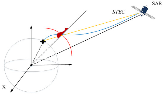
Figure 5. Ionospheric TEC distribution.

In order to estimate the ionospheric delay error, we use the global ionospheric TEC map provided by the European Center for Orbit Determination to estimate the total electron content. The ionospheric delay error is compensated for and corrected by calculating the position of the ionospheric puncture point.

2.5. Error of Image Processing

Imaging processing error mainly refers to the error caused by the imaging process, including the Go–Stop model error and elevation error.

2.5.1. Error of the Go–Stop Model

The LT-1 satellite imaging process mainly follows the traditional “Go–Stop” error model, which considers the satellite to be stationary at the time of signal transmission and reception. Thus, it is possible to ignore the satellite motion during the transmission and reception of the pulse and during the duration of the reception pulse; however, the satellite is actually moving. Therefore, imaging based on the above “Go–Stop” model will cause slant range error, which leads to inaccurate image geometric positioning accuracy [28].

The signal propagation process during imaging is illustrated in Figure 6. The sensor transmits a signal from position $P_t$, which travels through ${\tau }_1$ to reach point P and is reflected. After a time interval, the signal is received by the sensor, which is now located at position $P_r$ In the figure, $X_0$ denotes the initial azimuth position of the aperture, $t_t$ represents the total transmission time, and $t_r$ indicates the total reception time. During the transmission of the pulse signal, the sensor platform moves from point A to point B. During the reception of the pulse, the platform moves from point C to point D. That is, the sensor undergoes azimuthal movement throughout the entire transmission and reception process. Overall, the azimuthal movement during sensor transmission and reception results from two types of motion: platform movement within the bidirectional signal delay time and internal platform motion during signal transmission or reception. From Figure 6, we can derive the following system of equations:

$$\left\{\begin{array}{l}{\left(X_0+v{t}_r\right)}^2+{R_s}^2={\left(c{\tau }_2\right)}^2\\ {\left(X_0+v{t}_t\right)}^2+{R_s}^2={\left(c{\tau }_1\right)}^2\\ \tau ={\tau }_1+{\tau }_2\\ t_t+\tau =t_r\end{array}\right.$$

(12)

where $\tau$ denotes the round-trip delay and c denotes the signal propagation speed.

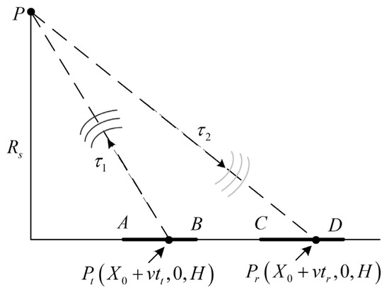
Figure 6. Satellite motion diagram.

In this paper, the zero Doppler moment is used as the azimuthal time of the signal when processing the data of the LT-1 satellite because the zero Doppler moment is very close to half of the pulse transmission time and the pulse reception time. That is, the “Intermediate time” model, as shown in Figure 7, can avoid the “Go–Stop” model caused by the error.

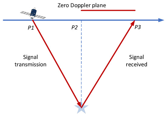
Figure 7. Schematic diagram of the “Go–Stop” model.

The azimuth time correction for the satellite’s motion from the pulse transmission time to the echo reception time is:

$$t_1=t_{raw}-{\tau }_{ref}/2$$

(13)

where $t_{raw}$ is the azimuth-to-time conversion factor and ${\tau }_{ref}$ is the round-trip propagation time for the target on the reference slant range. During the satellite’s internal platform motion while transmitting or receiving signals, echoes from near-end targets are received first, while echoes from far-end targets are received last. Therefore, for targets on the same distance line, the variation in reception time between near-end and far-end targets is precisely half the distance–time difference across the entire mapping bandwidth. This induces azimuth skew in the distance–time variation, resulting in residual azimuth observation time differences for targets at arbitrary slant ranges relative to the reference slant range target:

$$\Delta t_{Tar}={\displaystyle \frac{1}{2}}\cdot \left({\tau }_{Tar}-{\tau }_{ref}\right)$$

(14)

where ${\tau }_{Tar}$ represents the round-trip propagation time for the observation target. Compensating for this residual component in Equation (13) eliminates the azimuth bias effect. Taking LT-1 data as an example, failure to compensate for the Go–Stop effect would result in a displacement of approximately 20–30 m.

2.5.2. Error of Elevation

In order to achieve accurate geometric positioning accuracy of SAR images, elevation error must be considered. The positioning error caused by elevation error will cause image distortion, and the smaller the incident angle, the greater the elevation error. In this paper, a high-precision digital elevation model (DEM), the 5 m Precision DEM, is introduced to compensate for the elevation error.

3. Results and Discussion

Following its launch in 2022, the LT-1 satellite underwent eight months of in-orbit testing. Since its launch, the China Resources Satellite Application Center has conducted annual calibration missions at the Hami Calibration Site in Xinjiang and the Sunite Right Banner Calibration Site in Inner Mongolia (as shown in Figure 8). Throughout these calibration missions, to better monitor various image performance metrics, multiple angle-adjustable corner reflectors and active calibrators were uniformly deployed along the range and azimuth directions at specific intervals, tailored to the resolution and swath width of different imaging modes. Additionally, during each annual calibration mission, transiting imaging at the Surat Basin site in Queensland, Australia, is scheduled as needed. When the satellite passes over calibration sites, the corner reflectors and active calibrators appear as sharply focused bright points in the imagery, as shown in Figure 9.

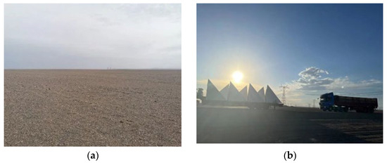
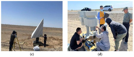
Figure 8. Placement of calibration sites and control points: (a) Xinjiang Hami calibration field; (b) Inner Mongolia calibration field; (c) corner reflector adjustment in outfield; (d) installation and commissioning of an active calibrator.

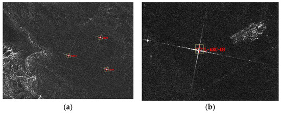
Figure 9. Schematic diagram of point target imaging: (a) corner reflector imaging; (b) active calibrator imaging.

Test data were selected from relatively stable images captured by the LT-1 satellite during its calibration period from 2022 to 2024. During testing, situations may arise where a single image fails to cover all observation point targets. In such cases, two adjacent scenes must be tested to achieve full coverage of all point targets. Ultimately, 54 scenes were selected, with the annual image acquisition timelines detailed in Table 3, Table 4 and Table 5.

Table 3. LT-1 data acquisition schedule in 2022.

Year	Satellite	Collection Date	Number of Images	Region
2022	LT-1A	27 April	9	Australia
		17 May		Australia
		27 May		Australia
		31 August		Hami, Xinjiang
		2 September		Hami, Xinjiang
		27 October		Hami, Xinjiang
	LT-1B	17 May	9	Australia
		18 May		Australia
		31 August		Hami, Xinjiang
		23 September		Hami, Xinjiang
		27 October		Hami, Xinjiang

Table 4. LT-1 data acquisition schedule in 2023.

Year	Satellite	Collection Date	Number of Images	Region
2023	LT-1A	17 October	9	Australia
		25 October		Australia
		6 November		Australia
		12 November		Sunit, Inner Mongolia
		2 December		Sunit, Inner Mongolia
		24 December		Sunit, Inner Mongolia
	LT-1B	16 October	9	Hami, Xinjiang
		25 October		Hami, Xinjiang
		11 November		Hami, Xinjiang
		19 November		Sunit, Inner Mongolia
		3 December		Sunit, Inner Mongolia

Table 5. LT-1 data acquisition schedule in 2024.

Year	Satellite	Collection Date	Number of Images	Region
2024	LT-1A	12 October	9	Hami, Xinjiang
		20 October		Sunit, Inner Mongolia
		28 October		Hami, Xinjiang
		11 November		Sunit, Inner Mongolia
		13 November		Sunit, Inner Mongolia
		17 November		Hami, Xinjiang
	LT-1B	12 October	9	Hami, Xinjiang
		16 October		Sunit, Inner Mongolia
		20 October		Sunit, Inner Mongolia
		1 November		Hami, Xinjiang
		11 November		Sunit, Inner Mongolia

The 2022 image data were calibrated using sites in Australia and Hami, Xinjiang, while the 2023 and 2024 image data utilized sites in Hami, Xinjiang, and Suniite Right Banner, Inner Mongolia. A total of 39 corner reflectors and active calibrators were covered. Partial imagery of corner reflectors and active calibrators from three calibration sites is shown in Figure 10. The left panel depicts the Australian calibration site, the upper right shows the Hami calibration site in Xinjiang, and the lower right shows the Sunite Right Banner calibration site in Inner Mongolia.

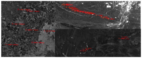
Figure 10. Control point imaging schematic.

When calculating the geometric positioning accuracy, the position of the corner reflector and the active scaler in the range of the intercepted image is the point target, the index corresponding to each point target is calculated separately, and the average value is taken as the final index result according to the date. According to the calculation results, the time series diagram can be drawn as shown in Figure 11.

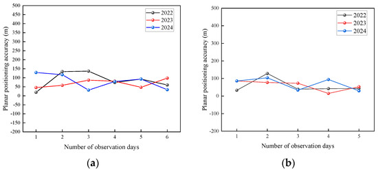
Figure 11. Planar positioning accuracy indicator results: (a) LT-1A plane positioning accuracy; (b) LT-1B plane positioning accuracy.

3.1. Comparative Analysis of Test Index and Design Index

According to the on-orbit test requirements of the LT-1 satellite, the imaging index of geometric positioning accuracy is better than 150 m in the interferometric wave position and 230 m in the extended wave position. The test data were analyzed, and the results are shown in Table 6. The analysis shows that in 2022, the maximum geometric positioning accuracy of the LT-1A image is 134.06 m, the minimum is 19.32 m, and the average is 86.08m; the maximum geometric positioning accuracy of the LT-1B image is 128.64 m, the minimum is 32.97 m, and the average is 57.25 m. In 2023, the maximum geometric positioning accuracy of the LT-1A image is 97.93 m, the minimum is 45.67 m, and the average is 69.42 m; the maximum geometric positioning accuracy of the LT-1B image is 86.02 m, the minimum is 14.95 m, and the average is 60.83 m. In 2024, the maximum geometric positioning accuracy of the LT-1A image is 129.19 m, the minimum is 31.55 m, and the average is 80.57 m; the maximum geometric positioning accuracy of the LT-1B image is 104.12 m, the minimum is 29.62 m, and the average is 69.54 m.

Table 6. LT-1 indicator test results.

Satellite	LT-1A			LT-1B
Time/year	2022	2023	2024	2022	2023	2024
Maximum/m	134.06	97.93	129.19	128.64	86.02	104.12
Minimum/m	19.32	45.67	31.55	32.97	14.95	29.62
Average/m	86.08	69.42	80.57	57.25	60.83	69.54

In summary, the image geometric positioning accuracy of the LT-1A and LT-1B satellites in the three years of in-orbit operation meets the requirements of in-orbit test indicators. The average positioning accuracy of the geometric plane is between 50 m and 90 m without precise geometric correction.

3.2. Analysis of Index Stability

In order to analyze the stability of the point target geometric positioning accuracy index in a time series, the standard deviation of the geometric positioning accuracy index of the annual image data can be calculated and normalized as the Stability Index. The formula for calculating the standard deviation is:

$$\sigma =\sqrt{{\displaystyle \frac{{{\displaystyle \sum _i^n\left(x_i-\overline{X}\right)}}^2}{n}}}$$

(15)

where n is the sample size and $\overline{X}$ is the sample mean.

The geometric positioning accuracy stability of the LT-1A and LT-1B satellites for the period 2022–2024 was calculated, as shown in Figure 12 below.

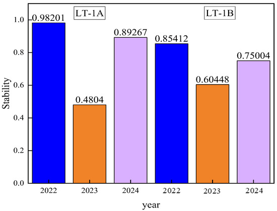
Figure 12. Geometric positioning accuracy standard deviation.

It can be seen from Figure 12 that the geometric positioning accuracy of the LT-1 satellite between the two satellites remained relatively stable from 2022 to 2024, and the planar positioning accuracy in 2023 was more stable compared to that in 2022 and 2024.

3.3. Geometric Precision Correction Positioning Accuracy

Based on the analysis of the accuracy of uncontrolled plane positioning in the above images, geometric positioning accuracy compensation was performed considering the end-to-end errors presented in Section 2. The results presented here are derived from four days of collected data. The geometric positioning accuracy obtained after fine correction is shown in Figure 13 below. It can be observed that after fine calibration, the error in the distance direction after compensation can be reduced to approximately 2.1 m, and the error in the azimuth direction after compensation can be reduced to approximately 1.3 m. That is, after compensation, the uncontrolled plane positioning accuracy of the image is significantly improved in both the distance and azimuth directions, achieving better than 3.0 m. Figure 14 illustrates the improvement in geometric positioning accuracy before and after calibration for three point targets. The green dots indicated by red arrows represent the actual latitude and longitude of the point targets. It can be observed that after fine calibration, the clearly focused point targets are closer to the actual latitude and longitude of the point targets.

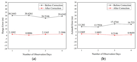
Figure 13. Geometric positioning accuracy after fine calibration: (a) comparison of range error after precise correction and compensation; (b) comparison of azimuth error after precise correction and compensation.

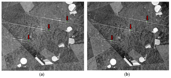
Figure 14. Schematic diagrams before and after geometric positioning accuracy compensation: (a) before compensation; (b) after compensation.

Compared to international L-band SAR systems, the LT-1 satellite’s geometry positioning accuracy after fine calibration significantly surpasses that of Japan’s ALOS-1 and approaches the geometry positioning accuracy of Italy’s COSMO-SkyMed. This demonstrates that the LT-1 system achieves high geometric fidelity through comprehensive error source analysis and compensation, supporting mission applications requiring high precision. These include feature extraction, high-precision imaging, and echo analysis of targets, enabling the provision of high-resolution imagery for in-orbit target areas.

4. Conclusions

As the first interferometric SAR satellite in China, L-band SAR image data play an important role in military and civil fields. In order to better analyze the application of satellite data in different scenarios and provide a reference basis, this paper analyzes the geometric positioning error sources of the LT-1 satellite full-link system. The image data of the three calibration fields during the satellite in-orbit test are selected for uncontrolled plane positioning accuracy and stability evaluation and analysis, and the image error source compensation is performed to obtain the fine corrected image data. The results show the following:

• The image geometric positioning accuracy of the LT-1A and LT-1B satellites in orbit within three years meets the requirements of the index test, and the average geometric plane positioning accuracy is between 50 m and 90 m without geometric precision correction.
• The geometric positioning accuracy of the LT-1 satellite between the two satellites remained relatively stable from 2022 to 2024, and the planar positioning accuracy in 2023 was more stable compared to that in 2022 and 2024.
• After precise correction, the image positioning error can be reduced to about 2.1 m in range and 1.3 m in azimuth, and the geometric positioning accuracy is better than 3.0 m.
• Although this research yielded satisfactory test results for geometric positioning accuracy, there remains room for improvement. While the satellite’s planar positioning has achieved a high level of performance, the analysis of coupling effects among various errors and the seasonal trends in long-term image geometric positioning accuracy still requires further validation. With the increasing application of satellites, we will continue to conduct in-depth research in conjunction with calibration experiments, persistently address issues, and enhance satellite data processing and application services.

References

- Wiley, C.A. Synthetic Aperture Radar. IEEE Trans. 1985, 21, 440–443. [Google Scholar] [CrossRef]
- Deng, Y.; Zhao, F.; Wang, Y. Brief Analysis on the Development and Application of Spaceborne SAR. J. Radars 2012, 1, 1–10. [Google Scholar] [CrossRef]
- Zhang, Q.; Han, X.; Liu, J. Progress and development trend of space-borne synthetic aperture radar remote sensing. Spacecr. Eng. 2017, 26, 1–8. [Google Scholar]
- Jin, G.; Liu, K.; Liu, D. An Advanced Phase Synchronization Scheme for LT-1. IEEE Trans. Geosci. Remote Sens. 2019, 58, 1735–1746. [Google Scholar] [CrossRef]
- Deng, Y.; Wang, Y. Key technologies for spaceborne SAR payload of LuTan-1 satellite system. J. Geod. Geoinf. Sci. 2024, 53, 1881–1895. [Google Scholar]
- Jiao, Y.; Liu, K. The Synchronization Transceiver Design and Experimental Verification for the LuTan-1 SAR Satellite. Sensors 2020, 20, 1463. [Google Scholar] [CrossRef]
- Zhang, R.; Xiang, W.; Liu, G. Interferometric coherence and seasonal deformation characteristics analysis of saline soil based on Sentinel-1A time series imagery. J. Syst. Eng. Electron. 2021, 32, 1270–1283. [Google Scholar] [CrossRef]
- Liang, D.; Liu, K.; Zhang, H. A High-Accuracy Synchronization Phase-Compensation Method Based on Kalman Filter for Bistatic Synthetic Aperture Radar. IEEE Geosci. Remote Sens. Lett. 2020, 17, 1722–1726. [Google Scholar] [CrossRef]
- Chen, J.; Li, W. Recent progress and trend of foreign SAR satellites. Shanghai Aerosp. 2016, 33, 1–19. [Google Scholar]
- Lou, L.; Liu, Z.; Zhang, H. Design and implementation of TH-2 satellite project. J. Geod. Geoinf. Sci. 2020, 49, 1252–1264. [Google Scholar]
- Li, S.; Ye, Y.; Fan, W. Analysis on positioning accuracy of TH-2 satellite system. J. Geod. Geoinf. Sci. 2022, 51, 2481–2492. [Google Scholar]
- Mohr, J.J.; Madsen, S.N. Geometric calibration of ERS satellite SAR images. IEEE Trans. Geosci. Remote Sens. 2001, 39, 842–850. [Google Scholar] [CrossRef]
- Rosenqvist, A.; Shimada, M.; Ito, N. ALOS PALSAR: A Pathfinder Mission for Global-Scale Monitoring of the Environment. IEEE Trans. Geosci. Remote Sens. 2007, 45, 3307–3316. [Google Scholar] [CrossRef]
- Covello, F.; Battazza, F.; Coletta, A. COSMO-SkyMed an existing opportunity for observing the Earth. J. Geodyn. 2010, 49, 171–180. [Google Scholar] [CrossRef]
- Eineder, M.; Minet, C.; Steigenberger, P. Imaging Geodesy—Toward Centimeter-Level Ranging Accuracy with TerraSAR-X. IEEE Trans. Geosci. Remote Sens. 2011, 49, 661–671. [Google Scholar] [CrossRef]
- Zhang, R.; Jiang, X. System Design and In-orbit Verification of the HJ-1C SAR Satellite. J. Radars 2014, 3, 249–255. [Google Scholar] [CrossRef]
- Jiayin, L.; Xiaolan, Q.; Yuxin, H. Geolocation of HJ-1C Satellite Image Using One Gcp. In Proceedings of the 2014 IEEE Geoscience and Remote Sensing Symposium, Quebec City, QC, Canada, 13–18 July 2014; pp. 4458–5229. [Google Scholar]
- Ding, C.; Liu, J.; Lei, B. Preliminary Exploration of Systematic Geolocation Accuracy of GF-3 SAR Satellite System. J. Radars 2017, 6, 11–16. [Google Scholar]
- Lin, M.; Yuan, X.; Liu, J.; Ye, X.; Zhang, Q. Application of gf-3 satellite monitoring typhoon. Spacecr. Eng. 2017. [Google Scholar]
- Zhang, Q. General design and key technologies of GF-3 satellite. J. Geod. Geoinf. Sci. 2017, 46, 269–277. [Google Scholar]
- Deng, Y.; Yu, W.; Zhang, H. Development trend of future spaceborne SAR technology. J. Radars 2020, 9, 33. [Google Scholar]
- Dang, H.; Tan, X. Review of spaceborne microwave remote sensing technology. Space Electron. Technol. 2025, 22, 35–49. [Google Scholar]
- Li, J.; Tan, X.; Li, C.; You, D. A review of development of GEO SAR technology. Space Electron. Technol. 2025, 22, 11–27. [Google Scholar]
- Wang, X.; Qi, R.; Yao, X. High-precision Simulation of Dynamic Oceans Synthetic Aperture Radar Imaging and Its Typical Application. J. Radars 2025, 14, 712–734. [Google Scholar]
- Yoon, Y.T.; Eineder, M.; Yague-Martinez, N. TerraSAR-X Precise Trajectory Estimation and Quality Assessment. IEEE Trans. Geosci. Remote Sens. 2009, 47, 1859–1868. [Google Scholar] [CrossRef]
- Milbert, D. Solid Earth Tide, FORTRAN Computer Program. Available online: http://geodesyworld.github.io/SOFTS/solid.htm (accessed on 15 August 2025).
- Cao, Y.; Jonsson, S. Advanced Insar tropospheric corrections from global atmospheric models that incorporate spatial stochastic properties of the troposphere. J. Geophys. Res. Solid Earth 2021, 126, e2020JB020952. [Google Scholar] [CrossRef]
- Qiu, X.; Han, C.; Liu, J. A Method for Spaceborne SAR Geolocation Based on Continuously Moving Geometry. J. Radar 2013, 54–59. [Google Scholar] [CrossRef]
Disclaimer/Publisher’s Note: The statements, opinions and data contained in all publications are solely those of the individual author(s) and contributor(s) and not of MDPI and/or the editor(s). MDPI and/or the editor(s) disclaim responsibility for any injury to people or property resulting from any ideas, methods, instructions or products referred to in the content. |
© 2025 by the authors. Licensee MDPI, Basel, Switzerland. This article is an open access article distributed under the terms and conditions of the Creative Commons Attribution (CC BY) license (https://creativecommons.org/licenses/by/4.0/).