Highlights
What are the main findings?
- The proposed SCGEM accurately delineates glacier boundaries under clouds, with the highest IoU of 0.7700.
- Both the generative adversarial mechanism and multi-task architecture notably improved the glacier boundary delineation accuracy under cloud cover.
What is the implication of the main finding?
- The Topo., SAR, and Tempo. features all contribute to glacier extraction in cloudy areas, with the Tempo. features contributing the most.
- The proposed architecture serves both to data clean and enhance the extraction of glacier texture features.
Abstract
Accurate delineation of glacier extent is crucial for monitoring glacier degradation in the context of global warming. Satellite remote sensing with high spatial and temporal resolution offers an effective approach for large-scale glacier mapping. However, persistent cloud cover limits its application on the Tibetan Plateau, leading to substantial omissions in glacier identification. Therefore, this study proposed a novel sub-cloudy glacier extraction model (SCGEM) designed to extract glacier boundaries from cloud-affected satellite images. First, the cloud-insensitive characteristics of topo-graphic (Topo.), synthetic aperture radar (SAR), and temporal (Tempo.) features were investigated for extracting glaciers under cloud conditions. Then, a transformer-based generative adversarial network (GAN) was proposed, which incorporates an image reconstruction and an adversarial branch to improve glacier extraction accuracy under cloud cover. Experimental results demonstrated that the proposed SCGEM achieved significant improvements with an IoU of 0.7700 and an F1 score of 0.8700. The Topo., SAR, and Tempo. features all contributed to glacier extraction in cloudy areas, with the Tempo. features contributing the most. Ablation studies further confirmed that both the adversarial training mechanism and the multi-task architecture contributed notably to improving the extraction accuracy. The proposed architecture serves both to data clean and enhance the extraction of glacier texture features.
1. Introduction
Glaciers are persistent ice bodies formed through processes such as snow accumulation, compaction, recrystallization, and refreezing. The Qinghai–Tibet Plateau (QTP) contains the largest reserves of ice and permafrost outside the polar regions, often referred to as the “Water Tower of Asia”. In recent years, widespread glacier retreat across the QTP has led to reduced river discharge in glacier-fed catchments [1]. Continued glacier shrinkage will further diminish contributions to downstream rivers, exacerbating freshwater scarcity in downstream urban areas [2]. Therefore, accurate and timely glacier extraction are critical for water resource protection and sustainable development in downstream basins.
Remote sensing technology provides large-scale, continuous observations that enable the mapping of glaciers and the detection of changes, supporting the development of inventories. Several essential glacier inventory datasets have been developed based on remote sensing including the Glacier Area Mapping for Discharge from the Asian Mountains (GAMDAM) [3], the Chinese Glacier Inventory (CGI) [4], and the Randolph Glacier Inventory (RGI) [5]. However, these inventories typically suffer from extended update intervals. The persistent cloud cover and seasonal snow accumulation create complex satellite observation conditions in the QTP. Therefore, developing automated extraction methods to overcome cloud effects is essential for improving glacier mapping accuracy and renewing the inventory.
A significant challenge in this context is identifying cloud-insensitive features that can characterize glaciers and distinguish their contributions. The commonly used SAR [6], topographic, and temporal features are not affected by cloud cover, but their ability to distinguish glaciers and other surfaces remains unclear. SAR data have been extensively applied in glacier studies [7], but some surface echoes are similar to the SAR echoes of glaciers. Topographic features offer complementary insights into glacier occurrence and development, but glaciers can develop in any terrain. Glaciers exhibit distinctive temporal patterns [8,9], making temporal features a promising alternative for mapping under cloudy conditions. However, the large volume and temporal discontinuity of temporal datasets hinder the effective extraction of representative temporal features. Therefore, it is necessary to develop time-series feature extraction methods and analyze the relative contributions of different types of features to glacier delineation under cloud-covered conditions.
Subsequently, identifying methods that can effectively depict glacier spatial detail remains a key challenge. The object-based image analysis [10] and snow-indicator method [11] glacier extraction approaches have proven effective in traditional glacier mapping. However, these methods rely on single-source features, which exhibit limited robustness in cloud-affected scenes and fail to fully utilize the texture feature detail. Deep learning models [12] have shown effectiveness in integrating heterogeneous multi-data sources. However, convolutional neural networks (CNNs) [13,14,15] are constrained by their fixed receptive fields, which limit their ability to capture spatially discontinuous information, particularly in fragmented optical imagery. Vision transformers (ViTs) [16] have been applied to glacier mapping due to their capacity to model long-range dependencies. However, the absence of explicit positional encoding weakens their ability to capture geographic correlations, which hinders the accurate delineation of glaciers. To address these limitations, enhancing the ViT framework for improved glacier texture feature extraction is essential to better represent the morphological characteristics of glaciers.
Due to the contamination in optical images, effectively identifying glaciers using a transformer-based method in cloud-covered regions remains a significant challenge. Traditional workflows often rely on selecting or synthesizing cloud-free images before extracting glaciers [17,18]. However, extracting glacier boundaries from reconstructed images introduces additional errors and increases computational cost. The more effective approach is to reconstruct cloud-free images and extract glaciers simultaneously, integrating both tasks within a single model. Recent advances in multi-task networks [19] have demonstrated strong performance and efficiency by sharing features across tasks, providing a viable framework for direct glacier extraction. By introducing a glacier reconstruction branch to guide the main extraction task, the model can reduce noise introduced during image reconstruction. Moreover, the generative adversarial network (GAN) structure employs a discriminator to assess the similarity between generated and real images. In the glacier extraction task, this structure can further constrain the feature filtering and learning of cloudy glaciers, improving the extraction accuracy under cloudy conditions. Integrating multi-task networks with a generative adversarial framework into a novel model represents the primary challenge of this study.
Therefore, this study proposed a multi-task GAN with a transformer-based backbone named the sub-cloud glacier extraction model. The proposed model selected three cloud-intensive features and tested the performance of each feature combination. The multi-task decoder and the GAN structure were introduced to guide the model in learning the distribution of glacier features under cloudy conditions. Finally, the proposed model was developed to extract glacier extent under heavy cloud cover in the Yarlung Zangbo River Basin region.
2. Study Area and Material
2.1. Study Area
The Yarlung Zangbo River Basin, situated on the southern QTP, is the world’s highest large river basin (Figure 1). Originating from the Gyima Yangzong Glacier in western Tibet, it flows eastward across the QTP before turning south through the Eastern Himalayas into India and Bangladesh. The basin is characterized by complex topography, with elevations ranging from over 5000 m on the Tibetan Plateau to less than 100 m in the lower reaches. The Basin region has 7523 glaciers according to the CGI, which is the ideal region for model experiment and verification.
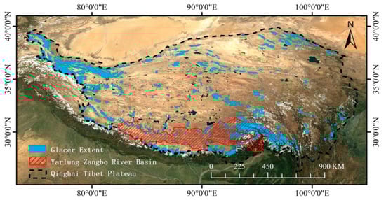
Figure 1.
The sturdy area with glacier extent.
2.2. Remote Sensing Data
Five types of datasets were utilized including spectral (Spec.), SAR imagery, topographic, cloudiness score (CS), and temporal parameters (Table 1). All features could be downloaded from the Google Earth Engine (GEE) platform [20]. Spectral bands and related indicators are commonly used features for glacier extraction and mapping. In this study, six spectral bands from Sentinel-2 (B2, B3, B4, B5, B8, and B11) and the normalized difference snow index (NDSI) were selected as spectral (Spec.) features, resulting in a total of seven channels. SAR data were obtained from Sentinel-1, with a 10 m resolution and two polarization channels (‘VV’ and ‘VH’). Tempo. features were extracted from spectral bands and indices over a three-year period to mitigate the effects of missing data, encompassing a total of 21 channels. Additionally, topographic information was represented by three key parameters: elevation, slope, and aspect. Finally, the Sentinel-2 cloud product provided supplementary information on cloud coverage, supporting both image reconstruction and glacier extraction tasks.

Table 1.
The features used in the glacier extraction study.
2.3. Training Samples
This study selected five regions to construct the training, testing, and validation datasets, covering a total area of approximately 4849.66 km2 (Table 2). Glacier samples were sourced from the CGI-2 and subsequently refined through manual correction based on Sentinel-2 images in the year 2020. The remote sensing features were divided into 64 × 64-pixel patches, resulting in 10,000 training patches and 2500 validation patches. Additionally, an independent testing area located at coordinates (90.026° E, 29.920° N) was selected for model comparison, with a total area of 498.07 km2.
Table 2.
The details of the training and validation datasets.
2.4. Data Preprocess
Images with more than 40% cloud cover were selected as the training dataset, while those with the lowest cloud cover were used as the ground truth. The spectral image was acquired between June and October, corresponding to the period of maximum seasonal glacier ablation and thus capturing the minimum glacier extent of the year. The slope and aspect were derived from the digital elevation model (DEM) using standard terrain analysis techniques. All the Topo., Tempo., and SAR features were clipped to a consistent spatial extent to ensure uniform coverage across datasets.
This study utilized the harmonic analysis and Fourier functions [21,22] to decompose periodic components from the Tempo. signal and extract features. The three key Tempo. parameters (phase, amplitude, and baseline shifts) can be calculated using the following equation:
where denotes the angular frequency, denotes the number of harmonics. denotes baseline shift of the indicator. denotes the amplitude of the indicator. denotes the Phase of the indicator. A glacier typically exhibits a cyclical pattern of annual variation. As a result, this study employed a one-year cycle for Fourier decomposition, with the harmonic number set to n = 1, and the angular frequency set to . All the spectral and indicator features were used to calculate three key parameters, resulting in 21 channels.
3. Methodology
3.1. Model Structure
This study proposed a multi-task GAN model that simultaneously reconstructs cloud-free images and extracts glacier boundaries. The proposed model employs a ViT-B backbone, incorporating an enhanced encoder, a CNN-based discriminator, and two decoder structures to jointly perform image reconstruction and glacier boundary extraction. The encoder was refined to enhance the ability to capture glacier-specific spatial information and semantic features. The multi-decoder structure enables the reconstruction branch to guide the model in learning texture and extracting glacier boundaries with a shared parameter encoder. The discriminator performs feature refinement across spatial and channel dimensions by assessing the similarity between generated and real images, effectively suppressing cloud-induced spurious features. The combination of multi-decoder structure and adversarial training provides clear glacier texture priors and suppresses cloud-induced noise, enhancing glacier boundary delineation under cloud cover.
The enhanced encoder has a reduced depth (4 transformer blocks) for computational efficiency while maintaining the original embedding dimension (768) and number of attention heads (12) (Figure 2). The overlap encoder expands the input into 49 tokens by introducing overlapping patches compared with the original 16 tokens. The discriminator employs a six-layer convolutional neural network, which determines the spatial and channel distribution consistency of the generated and real remote sensing images simultaneously.
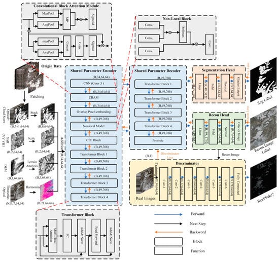
Figure 2.
The structure of the proposed SCGEM.
3.1.1. Encoder
The proposed encoder employs multi-head self-attention (MHSA) to capture semantic correlations, convolutional block attention module (CBAM) to enhance features and structural details, the non-local (NL) block for global glacier modeling, and convolutional position encoding (CPE) to strengthen positional representation.
- Multi-Head Self-Attention
The model employs MHSA to effectively capture global dependencies effectively, thereby enhancing robustness to interference and adaptability to multi-source data for accurate glacier extraction. The MHSA mechanism projects this sequence into queries, keys, and values using learnable linear mappings:
Each attention head computes scaled dot-product attention is expressed as:
Multiple heads are computed in parallel and concatenated is expressed as:
- Convolutional Block Attention Module
This study utilized CBAM with a slit CNN to jointly enhance Spatial and Channel dependencies. The Channel Attention block adaptively strengthens glacier features effectively and enhances the discrimination of multi-source features for glacier extraction. Given an intermediate feature map , the channel attention map is computed as:
where denotes the sigmoid function. The Spatial Attention block highlights key glacier spatial structure, improving extraction accuracy by suppressing background noise, where the spatial attention map is expressed as:
By sequentially applying channel and spatial attention, CBAM adaptively refines the intermediate features:
where ⊗ denotes element-wise multiplication with broadcasting.
- Non-Local block
The NL block establishes relationships across all spatial positions with global feature interactions, which enhance the contextual capture and the ability of glaciers to spatial structures. The block is defined as:
where, denotes measures similarity, this study utilized Gaussian similarity.
Then, the NLB fused a residual connection as the final output:
- Convolutional Position Encoding block
The CPE block injects spatial context into Transformer inputs, preserving local structure and enhancing the recognition of glacier boundaries and textures in multi-source imagery. The CPE block is expressed as:
where, represents a depthwise convolution with kernel size k, which encodes local spatial information into the feature map, thereby complementing the global attention of the transformer with fine-grained positional cues crucial for accurate glacier delineation.
3.1.2. Discriminator (Dis.)
The discriminator evaluates the similarity between the two images generated and real images, guiding the encoder to produce authentic features while suppressing cloud-induced artifacts. The discriminator utilizes a six-layer CNN, which enables multi-scale feature extraction and balances model complexity with training stability. Furthermore, the discriminator performs feature refinement across spatial and channel dimensions, improving the reliability of feature representations. By constraining the reconstruction branch, the discriminator strengthens the extraction branch to accurately extract glacier boundaries. Additionally, adversarial training reinforces feature fidelity and robustness, ensuring more reliable glacier extraction under challenging conditions.
3.1.3. Decoder
This study utilized a multi-task decoder architecture comprising a segmentation decoder and a reconstruction decoder. The segmentation decoder is the primary task of the proposed model, which incorporates the reconstruction decoder to learn the underlying distribution and enhance the feature representation.
- Reconstruction (Recon.) Decoder
The reconstruction decoder is designed to generate a realistic remote sensing image, which consists of four transformer blocks, followed by a linear projection and a fold function to reconstruct the spatial outputs. The reconstruction decoder employs a linear head to regress patch tokens into 7-channel reconstructed image outputs, facilitating accurate image restoration. By sharing parameters with the segmentation decoder, it enables the latter to learn more about the distribution of real images during glacier extraction, thereby imposing additional constraints on the segmentation process. This joint learning mechanism enhances the ability to extract glacier extent under clouds by leveraging auxiliary features.
- Segmentation (Seg.) Decoder
The glacier extraction is the primary task in the proposed method, where all components of the reconstruction decoder and discriminator will impact the performance of the glacier extraction task. The segmentation decoder employs a dedicated linear head to generate patch-level class scores, which are then combined into a pixel-wise segmentation map for glacier segmentation and extraction.
3.1.4. Loss Function
The loss function of this study includes glacier extraction and segmentation loss, glacier image reconstruction loss, and the discriminative loss.
- Discriminator Loss
The Discriminator loss consists of the discriminative loss and the gradient penalty, which is formulated based on the Wasserstein GAN with Gradient Penalty (WGAN-GP) [23,24]. The Gradient Penalty aims to improve training stability and enforce the Lipschitz continuity of the discriminator. The overall loss is defined as:
The denotes the adversarial loss for the discriminator, which estimates the Wasserstein distance between the generated data distribution and the real data distribution . The first term encourages the generator to produce samples that maximize the discriminator’s response, while the second term penalizes the discriminator’s output on real data.
The represents the gradient penalty term, which enforces the 1-Lipschitz constraint by penalizing deviations of the gradient norm from , which was sampled from points interpolated between real and generated data, and is a hyperparameter controlling the strength of the regularization.
This formulation enables more stable training compared to traditional GAN by providing a gradient penalty.
- Generator Loss
The generator loss is defined as a weighted sum of three components: the adversarial loss , the segmentation loss , and the reconstruction loss . Mathematically, it can be expressed as:
where , , and are hyperparameters that control the relative importance of each loss component. The adversarial loss for the discriminator on real samples is defined as the negative expected output of the discriminator over the real data distribution :
The reconstruction loss is closely related to the accuracy of glacier extraction. The missing details and structural information in glacier image reconstruction are significantly more pronounced in the MSE function. Thus, the proposed method utilizes a combination of Structural Similarity Index Measure (SSIM) and perceptual (Perc.) loss [25] as the reconstruction loss :
The segmentation loss is formulated as the binary cross-entropy loss, which measures the discrepancy between the predicted probability and the ground truth label over N pixels:
3.2. Implementation Detail and Evaluation
The model was fully implemented on a NVIDIA 2070S and an A4000 GPU. During the training process, we employed the Adam optimizer with a learning rate of 1 × 10⁻⁵, and the batch size was set to 16. To evaluate the performance of the proposed model, this study utilized overall accuracy (OA), F1, Intersection over Union (IoU), and Recall indicators to assess glacier extraction.
where , , , and denote true positives, false positives, true negatives, and false negatives, respectively. The IoU and F1 score are more stringent accuracy evaluation metrics with greater emphasis on glacier extraction, whereas OA and Recall are considered of secondary importance.
4. Result
4.1. Feature Contribution
This study tested different feature combinations to analyze the performance (Topo., SAR, Tempo.) on glacier extraction (Figure 3). While each data type demonstrated a specific capability for glacier mapping, a single data source struggled to identify debris-covered glacier areas reliably. Tempo. features alone achieved good extraction performance but tended to increase false positive errors (Line 3, Column 7). The SAR feature caused factual negative errors in the picture (Columns 6, 8, 9). The “SAR & Tempo.” and “Topo. & Tempo.” combinations resulted in missing details of the glacier edges. All feature combinations achieved satisfactory mapping in partially obscured areas (third column ) and enabled the delineation of glaciers beneath cloud cover. To avoid the influence of stochastic fluctuations, model performance was evaluated using the average accuracy over the final ten training epochs.
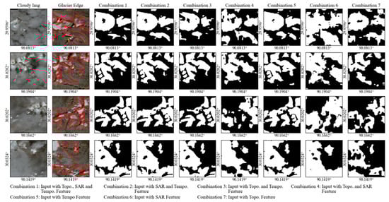
Figure 3.
Glacier boundary extraction results with different feature combinations. The first column indicates the cloudy image input. The second column shows the real images, with red lines denoting the manually delineated glacier boundaries. The third to ninth columns display the glacier extraction results with different feature combinations (Topo. & SAR & Tempo., SAR & Tempo., Topo. & Tempo., Topo. & SAR, Tempo., SAR, and Topo.). Black regions represent non-glacier areas, and white regions indicate glacier areas.
The accuracy assessment of glacier extraction with different feature combinations is presented in Table 3. The results show that using only the Topo. or SAR features achieved limited performance, with the lowest IoU values of 0.2877 and 0.2912, respectively. In contrast, the Tempo. feature achieved a substantially higher IoU of 0.6976. The combinations involving Tempo. features always outperformed, while the combination of Tempo. and SAR features achieved an IoU of 0.7523. Compared with the single feature, the combination of Tempo. and Topo. achieved an improved IoU (0.7225) over the single Tempo. feature but had a reduced recall (0.9208). The combination of SAR and Topo. improved over individual features but remained suboptimal, with an IoU of 0.3832. All three feature combinations achieved the best IoU (0.7700). The combination of SAR and Tempo. attained a decrease of 0.7523, accompanied by a slight decline in recall. The results suggest that the Tempo. features are most critical for glacier extraction under cloud conditions, SAR offers moderate complementary value, and Topo. features may have adverse effects on glacier extraction.
Table 3.
Glacier extraction accuracy with different feature combinations.
4.2. Model Efficiency
This paper utilized different levels of contaminated images to test the model efficiency (Figure 4). Due to the difficulty of acquiring images with various cloud cover, this paper introduced noise into the glacier extent to simulate cloud-contaminated conditions. The results indicate that the spatial structures of glaciers remained unchanged under different noise levels, and most glacier areas were accurately distinguished. In addition, noise tended to exacerbate the fragmentation of glacier boundaries in the fully noise-contaminated images. As the noise level increased, the model tended to use redundant features to infer the area of glaciers. Certain specific regions exhibited false positives in the glacier extraction results (Line 3, Column 7). Overall, although the noise level presented a certain influence on glacier extraction, the model demonstrated a notable capability to extract the glacier boundary in different cloud contamination levels.
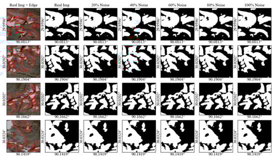
Figure 4.
Glacier extraction results under varying noise levels. The first column shows the real images, with red lines denoting the manually delineated glacier boundaries. The second to seventh columns show the extraction outcomes for different noise percentages (real image, 20%, 40%, 60%, 80%, and 100% noise), where black regions represent non-glacier areas and white regions denote glacier areas.
The glacier extraction accuracy exhibited a slight decreasing trend with increasing noise levels (Table 4). The model achieved the highest IoU (0.7828) in a non-cloudy image, but the lowest recall (0.9301). As the noise was introduced, the IoU, F1-score, and OA gradually declined as the noise level increased. The IoU changed only marginally (0.7772) with the 100% noise level, and both the F1 score and overall accuracy only showed a marginal decline in noise-contaminated images. These results demonstrate that the proposed model possesses substantial robustness against cloud-induced interference, ensuring reliable glacier extraction even under heavily contaminated conditions. The recall increased with the noise level, indicating that the model tends to overestimate the number of guessed regions.
Table 4.
Glacier extraction accuracy under different contamination conditions.
4.3. Ablation Study
The ablation study comprised three aspects: (1) testing the contribution of different encoder blocks, (2) adjusting the reconstruction loss for glacier extraction, and (3) evaluating the efficiency of GAN and multi-task architecture (Table 5). The encoder ablation applied MSE and perceptual loss and utilized all Topo., SAR, and Tempo. features, which evaluated the contributions of different block combinations. The CBAM module was coupled with the CNN backbone and jointly evaluated for the enhancement influence. Experimental results showed that integrating all four encoder blocks achieved the highest IoU (0.7537), indicating that each module contributed to the glacier extraction performance. The CPE module improved the IoU by 0.04 with the most effectiveness. Additionally, removing the CNN and CBAM led to an approximate 0.03 decrease in IoU, with the most important role in the encoder. Regarding reconstruction loss efficiency, the various combinations of reconstruction loss significantly influenced the glacier extraction performance. The combination of SSIM and perceptual loss achieved the highest IoU (0.7700) and recall (0.9394), while MSE loss yielded the lowest IoU (0.7243). Combining recon losses improved IoUs compared with the single loss, while incorporating perceptual loss consistently enhanced segmentation accuracy. In terms of structure efficiency, the model integrating both the reconstruction decoder and GAN achieved the highest IoU (0.7700). Models with only the glacier segmentation decoder yielded IoUs of 0.7102, and the reconstruction decoder had IoUs of 0.6715. The reduced IoUs indicate that both the multi-task and GAN structures enhanced the performance of the model, while the GAN structure contributed more substantially. Furthermore, compared with a 100% noise contaminated image, the model exhibited a slight decline in evaluation accuracy when using an actual cloudy image.
Table 5.
Ablation study for the proposed model.
4.4. Comparison Analysis
This study selected the traditional NDSI threshold method [18], several convolution-based models (RepVGG-B3 [26], YOLOv8-M), and transformer-based models (Mask2Former [27], ViT-B, Swin-S) and compared their performance in glacier extraction (Figure 5). The NDSI threshold method exhibited fragmented glacier extents, leading to false positive errors (Column 4). The convolution-based models detected excessively large glacier areas (Column 5, 6). The YOLOv8-M model preserved glacier edge details more effectively than the RepVGG-B3 model. In contrast, the transformer-based models generated smaller and more conservative glacier delineations. Both ViT-B and Swin-S achieved enhanced performance, but also produced a truth negative (Lines 3, Colomn 8, 9) of false positives (Lines 4, Colomn 8, 9) in detected glacier areas compared to the proposed model. The ViT-based models in the comparison generally failed to maintain glacier boundary details effectively.
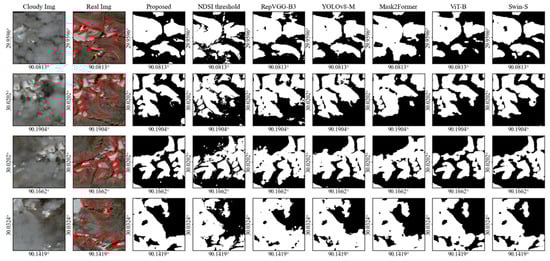
Figure 5.
Glacier extraction results with different models. The first column indicates the cloudy image input. The second column shows the real images, with red lines denoting the manually delineated glacier boundaries. The third to ninth columns show the glacier extraction results obtained using the various models (proposed, NDSI threshold, RepVGG-B3, YOLOv8-M, ViT-B, and Swin-S).
This study evaluated the accuracy of glacier extraction using different models (Table 6). The proposed model achieved the highest IOU (0.7700) among all of the compared models, while RepVGG-B3 achieved the lowest IoU with the reduced parameters and GFLOPs (1.24). The YOLOv8-M model achieved an IOU of 0.7034 with the fewest parameters, indicating higher potential compared with RepVGG-B3. Although our model introduced slightly more parameters, it achieved a higher accuracy than Mask2Former while requiring substantially fewer GFLOPs (1.35). Compared with the original ViT model, the proposed model reduced the number of parameters by 26 million, while the glacier extraction IoU improved by 0.06. The improvement can be attributed to a reduction in transformer blocks and an enhancement in feature extraction and architecture. The Swin-S model achieved the second-highest IoU (0.7447) while maintaining a low parameter count (24M). This superior performance can be attributed to the architecture design of the Swin transformer block, which significantly reduces the number of parameters and enhances multi-scale feature extraction. The pyramid structure of Swin Trans also shows excellent potential for further integration and optimization.
Table 6.
Glacier extraction accuracy with different models.
5. Discussion
5.1. The Cloud-Insensitive Features Properties
This study selected Topo., SAR, and Tempo., three cloud-insensitive features, and compared and evaluated their contributions to glacier extraction (Figure 6). Cloud cover substantially diminishes the separability of visible spectral bands for effectively distinguishing glaciers from other areas. The distribution of the visible bands (Figure 6a–c) and NDSI (Figure 6d) values showed limited separability, with a decrease in the difference in the mean values and a reduction in the concentration levels (Figure 6a–d). As a result, the visible spectral features showed limited effectiveness for glacier extraction alone. The Topo. features furnish critical information on elevation and terrain gradients, supporting morphological discrimination. However, the elevation and aspect features exhibited limited separability (Figure 6e,g). Glaciers generally exhibit lower mean slopes compared with the surrounding terrain (Figure 6f). However, the widely distributed glacier slope values limit the ability to delineate glacier extent. The SAR feature offers robust, all-weather imaging capabilities, conveying surface scattering and kinematic signals essential for differentiating glaciers from non-glacier areas. The VV polarization showed higher separability than VH, with glaciers exhibiting lower backscatter signals compared with non-glacier areas (Figure 6h,i). The mean backscatter (VV, VH) levels and the degree of clustering of SAR metrics were insufficient to enable accurate discrimination. As a result, the SAR and Topo. features exhibited limited performance when used independently for glacier delineation. The Tempo. features exhibited higher baseline values, lower amplitudes, and lower phases compared with other surface types (Figure 6j–l). This result demonstrated markedly greater differences in mean values and higher concentration levels compared with the other two features, making it the most effective for glacier extraction. Although both SAR and Topo. features presented inefficient performance alone, they provided structural and physical priors that substantially enhanced the accuracy and resilience of glacier mapping when combined with Tempo. features.
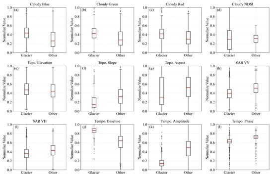
Figure 6.
The feature separability of glaciers under cloud cover. (a–d) indicates optical features with clouds (Blue, Green, Red, NDSI). (e–g) indicates Topo. features (elevation, slope, aspect); (h,i) indicates SAR backscattering features (VV, VH); (j–l) indicates Tempo. harmonic features (baseline, amplitude, phase). The distributions highlight varying degrees of separability between glaciers and other land cover types.
The Tempo. feature exhibited the highest discriminative capability (Figure 7). Glaciers experience diverse dynamic processes including melting, accumulation, and ice flow throughout the annual cycle. The satellite revisit cycle and the uncertain imaging conditions for each pixel complicate the incorporation of Tempo. information into machine learning frameworks. Harmonic functions provide a comprehensive description to extract Tempo. features, which encompass three parameters (phase, baseline, and amplitude) and effectively distinguish glaciers from other areas. Bare land typically exhibited low NDSI values, though precipitation-driven events in spring occasionally caused higher values (indicated by the yellow line). Ice lake (green line) exhibited a similar NDSI timeseries trend to glaciers, but with a higher amplitude. The NDSI of seasonal snow and glacier melt areas was driven by temperature, showing an increase in winter and a decrease during the summer period (green line). Bare land and seasonal snow both exhibited similar trends, but with a phase difference due to differing driving factors. In contrast, the timeseries NDSI of glaciers (blue line) and seasonal snow (red line) shared similar phases driven by temperature; however, the baseline and amplitude of the glacier NDSI were higher than those of seasonal snow and glacier melt areas, enabling their differentiation. Therefore, Tempo. features can effectively distinguish glaciers from seasonal snow areas and serve as a valuable attribute for glacier extraction.
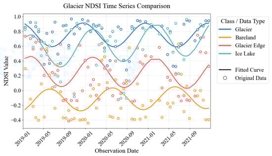
Figure 7.
The time series and fitted NDSI in glacier extraction. The vertical axis is the NDSI value, and the horizontal axis is the date of observations. The circle represents the original data, and the line represents the data fitted using the harmonic method. The blue, yellow, red, and green lines indicated the glacier, bare land, melting area of the glacier, and ice lake, respectively.
5.2. Contribution of the Model Architectural
The key enhancements in the proposed model center on two aspects: the generative adversarial and the multi-task decoder architecture. The GAN structure introduces an adversarial loss that encourages segmentation outputs to exhibit more natural texture, edges, and spatial distributions, effectively reducing block artifacts and blurred boundaries. Additionally, the discriminator introduced a data filtering and cleansing mechanism by identifying outputs that deviate from the actual data distribution. This is particularly beneficial for regions with cloud cover or poor data quality. The reconstruction decoder head provides an additional constraint by learning the mapping from multi-source features to authentic cloud-free remote sensing imagery. Through this reconstruction process, the model captures the spatial structural characteristics of real images. By sharing parameters between the two decoder branches, the glacier extraction task benefits from features that are more representative of genuine image content. Consequently, these structural enhancements contribute to improved accuracy in glacier delineation.
The image reconstruction loss exerted a significant influence on glacier extraction performance during the model training process. For glacier extraction, the model prioritizes structural and textural similarity over global spectral differences. Therefore, the commonly used MSE loss had minimal impact on glacier delineation in this study. In contrast, the SSIM loss enhanced sensitivity to glacier edges and textural details, thereby improving glacier boundary delineation. The perceptual loss captured both low-level image details and high-level semantic information, effectively facilitating the learning of structural features. Moreover, the combination of SSIM and perceptual losses enabled a more effective capture of the texture details and overall image structure, yielding the highest glacier extraction accuracy.
The enhanced encoder improves the glacier extraction performance by integrating multiple complementary blocks. The CPE block effectively captures local spatial positional relationships, preserving the underrepresented spatial context in traditional transformer blocks. The non-local block captures long-range dependencies and semantically related regions, facilitating the reconstruction of glacier details under cloud cover. The CBAM module strengthens feature representation by emphasizing informative features while suppressing irrelevant or redundant information. Furthermore, the hybrid CNN-transformer architecture combines local and global context modeling, enabling the network to capture complex spatial dependencies and further enhance the reliability of glacier extraction.
5.3. Comparison with Current Glacier Inventory
The comparison analysis of glacier extraction derived from different glacier inventories, including manual extraction (red line), model predictions (blue line), GLIMS inventory (green line), and the CGI inventory (yellow line), is shown in Figure 8. Across all regions (Figure 8a–f), the predicted boundaries generally showed a closer agreement with the manually labelled reference compared with GLIMS and CGI. The GLIMS glacier boundary was depicted in 2018 and presented less glacier extent than CGI, with more glacier fragmentation. The second CGI was produced in 2011, with the largest glacier area and the most complex boundary extraction. Because the glacier inventories were compiled at an earlier date, the GLIMS and CGI glacier outlines slightly exceeded the extent of the most recent glacier boundaries (Figure 8b–f). The temporal mismatches between inventory data acquisition and the satellite images caused discrepancies, indicating that the current glacier inventory needs to be updated promptly. In other cases, the proposed method had limited performance in debris-covered areas due to the confusion between seasonal snow and glaciers. Overall, the proposed method exhibited lower glacier fragmentation and reduced false positives in cloudy cover areas, achieving efficient glacier mapping. In addition, the proposed method exhibited enhanced adaptability to complex terrain and cloud-covered conditions, highlighting its potential contribution to the development of updated glacier inventories.
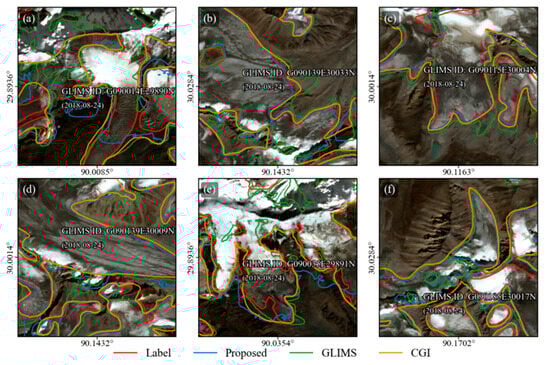
Figure 8.
Glacier boundary comparison with different glacier inventories. (a–f) shows several glacier boundaries overlaid on Sentinel-2 imagery. The red lines represent manually produced reference labels, the blue lines indicate the predicted glacier by the proposed model, the green lines correspond to the GLIMS glacier inventory, and the orange lines correspond to the CGI glacier inventory. The GLIMS glacier ID and GLIMS date are shown in the sub-figure.
6. Conclusions
This study developed a novel model (SCGEM) leveraging multi-temporal features to improve glacier mapping under cloudy conditions. The study analyzed the contributions of cloud-insensitive features including SAR, temporal, and topographic data. The Tempo. features were particularly effective in supporting glacier boundary delineation under cloud cover, whereas the SAR and Topo. features provided limited contributions. The proposed SCGEM achieved significant improvements with an IoU of 0.7700 and an F1 score of 0.8700. The SCGEM integrates a multi-task decoder and a generative adversarial framework, enabling the model to learn glacier textures and boundary details more effectively. These findings demonstrate that SCGEM can provide a robust tool for glacier mapping under persistent cloud conditions. Given the increasing cloud persistence in glacierized regions, SCGEM offers a practical solution for improving the accuracy and consistency of glacier extraction. This advancement is critical for refining glacier inventories and enhancing the assessments of cryospheric responses to climate change.
Author Contributions
Conceptualization, Y.C. and K.J.; Methodology, Y.C.; Writing—original draft preparation, Y.C.; Writing—review and editing, Y.C. and K.J.; Supervision, H.W., G.T., F.J., J.L., S.Q., L.Z., Z.J., X.G., L.G. and Q.W. All authors have read and agreed to the published version of the manuscript.
Funding
This work was supported by the National Key R&D Program of China (Grant No. 2024YFF1306200), the National Natural Science Foundation of China (Grant Nos. 42192580 and No.42192581), and the FengYun Application Pioneering Project (Grant No. FY-APP-2022.0307).
Data Availability Statement
Data are unavailable due to privacy or ethical restrictions.
Acknowledgments
During the preparation of this study, the authors used GPT4 for the purposes of code generation. The authors have reviewed and edited the output and take full responsibility for the content of this publication.
Conflicts of Interest
The authors declare no conflicts of interest.
Abbreviations
The following abbreviations are used in this manuscript:
| SCGEM | Sub-cloudy glacier extraction model |
| Topo. | Topographic |
| SAR | Synthetic aperture radar |
| Tempo. | Temporal |
| QTP | Qinghai–Tibet Plateau |
| GAMDAM | Glacier Area Mapping for Discharge from the Asian Mountains |
| CGI | Chinese Glacier Inventory |
| RGI | Randolph Glacier Inventory |
| CNNs | Convolutional neural networks |
| ViT | Vision transformers |
| GAN | Generative adversarial network |
| Spec. | Spectral |
| CS | Cloudiness score |
| NDSI | Normalized difference snow index |
| DEM | Digital elevation model |
| MHSA | Multi-head self-attention |
| CBAM | Convolutional block attention module |
| NL | Non-local |
| CPE | Convolutional position encoding |
| Dis. | Discriminator |
| Recon. | Reconstruction |
| Seg. | Segmentation |
| WGAN-GP | Wasserstein GAN with Gradient Penalty |
| OA | Overall accuracy |
| IoU | Intersection over Union |
References
- Wangchuk, S.; Bolch, T.; Robson, B.A. Monitoring glacial lake outburst flood susceptibility using Sentinel-1 SAR data, Google Earth Engine, and persistent scatterer interferometry. Remote Sens. Environ. 2022, 271, 112910. [Google Scholar] [CrossRef]
- You, Q.L.; Cai, Z.Y.; Pepin, N.; Chen, D.L.; Ahrens, B.; Jiang, Z.H.; Wu, F.Y.; Kang, S.C.; Zhang, R.N.; Wu, T.H.; et al. Warming amplification over the Arctic Pole and Third Pole: Trends, mechanisms and consequences. Earth-Sci. Rev. 2021, 217, 103625. [Google Scholar] [CrossRef]
- Nuimura, T.; Sakai, A.; Taniguchi, K.; Nagai, H.; Lamsal, D.; Tsutaki, S.; Kozawa, A.; Hoshina, Y.; Takenaka, S.; Omiya, S.; et al. The GAMDAM glacier inventory: A quality-controlled inventory of Asian glaciers. Cryosphere 2015, 9, 849–864. [Google Scholar] [CrossRef]
- Guo, W.Q.; Liu, S.Y.; Xu, L.; Wu, L.Z.; Shangguan, D.H.; Yao, X.J.; Wei, J.F.; Bao, W.J.; Yu, P.C.; Liu, Q.; et al. The second Chinese glacier inventory: Data, methods and results. J. Glaciol. 2015, 61, 357–372. [Google Scholar] [CrossRef]
- Pfeffer, W.T.; Arendt, A.A.; Bliss, A.; Bolch, T.; Cogley, J.G.; Gardner, A.S.; Hagen, J.O.; Hock, R.; Kaser, G.; Kienholz, C.; et al. The Randolph Glacier Inventory: A globally complete inventory of glaciers. J. Glaciol. 2014, 60, 537–552. [Google Scholar] [CrossRef]
- Zhu, Q.; Guo, H.; Zhang, L.; Liang, D.; Wu, Z.; Liu, Y.; Lv, Z. GLA-STDeepLab: SAR Enhancing Glacier and Ice Shelf Front Detection Using Swin-TransDeepLab With Global–Local Attention. IEEE Trans. Geosci. Remote Sens. 2023, 61, 1–13. [Google Scholar] [CrossRef]
- Zahriban Hesari, M.; Buono, A.; Nunziata, F.; Aulicino, G.; Migliaccio, M. Multi-Polarisation C-Band SAR Imagery to Estimate the Recent Dynamics of the d’Iberville Glacier. Remote Sens. 2022, 14, 5758. [Google Scholar] [CrossRef]
- Shi, Y.; Liu, G.; Wang, X.; Liu, Q.; Zhang, R.; Jia, H. Assessing the Glacier Boundaries in the Qinghai-Tibetan Plateau of China by Multi-Temporal Coherence Estimation with Sentinel-1A InSAR. Remote Sens. 2019, 11, 392. [Google Scholar] [CrossRef]
- Ke, L.H.; Zhang, J.S.; Fan, C.Y.; Zhou, J.J.; Song, C.Q. Large-Scale Monitoring of Glacier Surges by Integrating High-Temporal- and -Spatial-Resolution Satellite Observations: A Case Study in the Karakoram. Remote Sens. 2022, 14, 4668. [Google Scholar] [CrossRef]
- Mitkari, K.V.; Arora, M.K.; Tiwari, R.K.; Sofat, S.; Gusain, H.S.; Tiwari, S.P. Large-Scale Debris Cover Glacier Mapping Using Multisource Object-Based Image Analysis Approach. Remote Sens. 2022, 14, 3202. [Google Scholar] [CrossRef]
- Zhang, M.; Wang, X.; Shi, C.; Yan, D. Automated Glacier Extraction Index by Optimization of Red/SWIR and NIR/SWIR Ratio Index for Glacier Mapping Using Landsat Imagery. Water 2019, 11, 1223. [Google Scholar] [CrossRef]
- Chen, L.; Zhang, W.; Yi, Y.; Zhang, Z.; Chao, S. Long Time-Series Glacier Outlines in the Three-Rivers Headwater Region from 1986 to 2021 Based on Deep Learning. IEEE J. Sel. Top. Appl. Earth Obs. Remote Sens. 2022, 15, 5734–5752. [Google Scholar] [CrossRef]
- Periyasamy, M.; Davari, A.; Seehaus, T.; Braun, M.; Maier, A.; Christlein, V. How to Get the Most Out of U-Net for Glacier Calving Front Segmentation. IEEE J. Sel. Top. Appl. Earth Obs. Remote Sens. 2022, 15, 1712–1723. [Google Scholar] [CrossRef]
- Xie, Z.; Haritashya, U.K.; Asari, V.K.; Young, B.W.; Bishop, M.P.; Kargel, J.S. GlacierNet: A Deep-Learning Approach for Debris-Covered Glacier Mapping. IEEE Access 2020, 8, 83495–83510. [Google Scholar] [CrossRef]
- Mohajerani, Y.; Wood, M.; Velicogna, I.; Rignot, E. Detection of Glacier Calving Margins with Convolutional Neural Networks: A Case Study. Remote Sens. 2019, 11, 74. [Google Scholar] [CrossRef]
- Peng, Y.; He, J.; Yuan, Q.; Wang, S.; Chu, X.; Zhang, L. Automated glacier extraction using a Transformer based deep learning approach from multi-sensor remote sensing imagery. ISPRS J. Photogramm. Remote Sens. 2023, 202, 303–313. [Google Scholar] [CrossRef]
- Hu, M.; Zhou, G.; Lv, X.; Zhou, L.; He, X.; Tian, Z. A New Automatic Extraction Method for Glaciers on the Tibetan Plateau under Clouds, Shadows and Snow Cover. Remote Sens. 2022, 14, 3084. [Google Scholar] [CrossRef]
- Huang, L.; Li, Z.; Zhou, J.M.; Zhang, P. An automatic method for clean glacier and nonseasonal snow area change estimation in High Mountain Asia from 1990 to 2018. Remote Sens. Environ. 2021, 258, 112376. [Google Scholar] [CrossRef]
- Lin, L.; Liu, L.; Liu, M.; Zhang, Q.; Feng, M.; Khalil, Y.S.; Yin, F. DEDNet: Dual-Encoder DeeplabV3+ Network for Rock Glacier Recognition Based on Multispectral Remote Sensing Image. Remote Sens. 2024, 16, 2603. [Google Scholar] [CrossRef]
- Gorelick, N.; Hancher, M.; Dixon, M.; Ilyushchenko, S.; Thau, D.; Moore, R. Google Earth Engine: Planetary-scale geospatial analysis for everyone. Remote Sens. Environ. 2017, 202, 18–27. [Google Scholar] [CrossRef]
- Roerink, G.J.; Menenti, M.; Verhoef, W. Reconstructing cloudfree NDVI composites using Fourier analysis of time series. Int. J. Remote Sens. 2000, 21, 1911–1917. [Google Scholar] [CrossRef]
- Clark, M.L.; Aide, T.M.; Grau, H.R.; Riner, G. A scalable approach to mapping annual land cover at 250 m using MODIS time series data: A case study in the Dry Chaco ecoregion of South America. Remote Sens. Environ. 2010, 114, 2816–2832. [Google Scholar] [CrossRef]
- Gulrajani, I.; Ahmed, F.; Arjovsky, M.; Dumoulin, V.; Courville, A. Improved training of wasserstein GANs. In Proceedings of the Proceedings of the 31st International Conference on Neural Information Processing Systems, Long Beach, CA, USA, 4–9 December 2017; pp. 5769–5779. [Google Scholar]
- Wang, Y.M.; Peng, X.Y.; Huang, W.Q.; Ye, X.P.; Jiang, M.F. Self-supervised non-rigid structure from motion with improved training of Wasserstein GANs. IET Comput. Vis. 2023, 17, 404–414. [Google Scholar] [CrossRef]
- Johnson, J.; Alahi, A.; Li, F.F. Perceptual Losses for Real-Time Style Transfer and Super-Resolution. Comput. Vis.-ECCV 2016 2016, 9906, 694–711. [Google Scholar] [CrossRef]
- Ding, X.H.; Zhang, X.Y.; Ma, N.N.; Han, J.G.; Ding, G.G.; Sun, J. RepVGG: Making VGG-style ConvNets Great Again. In Proceedings of the 2021 IEEE/CVF Conference on Computer Vision and Pattern Recognition (CVPR), Nashville, TN, USA, 20–25 June 2021; pp. 13728–13737. [Google Scholar] [CrossRef]
- Cheng, B.W.; Misra, I.; Schwing, A.G.; Kirillov, A.; Girdhar, R. Masked-attention Mask Transformer for Universal Image Segmentation. In Proceedings of the 2022 IEEE/CVF Conference on Computer Vision and Pattern Recognition (Cvpr 2022), New Orleans, LA, USA, 18–24 June 2022; pp. 1280–1289. [Google Scholar] [CrossRef]


Disclaimer/Publisher’s Note: The statements, opinions and data contained in all publications are solely those of the individual author(s) and contributor(s) and not of MDPI and/or the editor(s). MDPI and/or the editor(s) disclaim responsibility for any injury to people or property resulting from any ideas, methods, instructions or products referred to in the content. |
© 2025 by the authors. Licensee MDPI, Basel, Switzerland. This article is an open access article distributed under the terms and conditions of the Creative Commons Attribution (CC BY) license (https://creativecommons.org/licenses/by/4.0/).