Highlights
What are the main findings?
- This article presents an image processing method to semi-automatically track wildfire progression.
- The algorithm was successfully applied to aerial infrared imagery acquired during tactical fire management operations.
What are the implications of the main finding?
- These results illustrate how tactical data can be used in fire behavior studies.
- The proposed method may facilitate real-time analysis of tactical information during wildfire emergencies.
Abstract
Remote sensing of wildland fires has become an integral part of fire science. Airborne sensors provide high spatial resolution and can provide high temporal resolution, enabling fire behavior monitoring at fine scales. Fire agencies frequently use airborne long-wave infrared (LWIR) imagery for fire monitoring and to aid in operational decision-making. While tactical remote sensing systems may differ from scientific instruments, our objective is to illustrate that operational support data has the capacity to aid scientific fire behavior studies and to facilitate the data analysis. We present an image processing algorithm that automatically delineates active fire edges in tactical LWIR orthomosaics. Several thresholding and edge detection methodologies were investigated and combined into a new algorithm. Our proposed method was tested on tactical LWIR imagery acquired during several fires in California in 2020 and compared to manually annotated mosaics. Jaccard index values ranged from 0.725 to 0.928. The semi-automated algorithm successfully extracted active fire edges over a wide range of image complexity. These results contribute to the integration of infrared fire observations captured during firefighting operations into scientific studies of fire spread and support landscape-scale fire behavior modeling efforts.
1. Introduction
Recent changes in wildland fire conditions and behavior have brought on new challenges in analyzing and modeling their dynamics. Manifestations of extreme fire behavior, such as rapid fire spread and high intensity [1,2], are further leading to unsafe conditions for firefighting operations and the public, accentuating the need for accurate fire behavior predictions. The fire spread component is at the foundation of fire behavior models, and the ability to improve model performance is a function of the data that is available.
Remote sensing of wildland fires has become an integral part of fire science due to its multiple applications, such as monitoring active fires, evaluating fire effects, estimating fire emissions, and assessing fire risk. Methods of calculating fire spread using ground devices [3,4] provide in situ measurements during laboratory and field experiments, while visual and infrared remote sensing camera systems provide continuous capture of a fire and a more flexible means of measuring fire spread when placement of ground devices may not be convenient or accessible.
Fire spread has been analyzed from spaceborne sensors such as the Moderate Resolution Infrared Sensor [5] and Landsat Thematic Mapper [6]. The consistent availability of spaceborne sensors makes them useful in pre- and post-fire monitoring. However, their low temporal resolution and susceptibility to smoke interference make them less suitable for measuring fine-scale fire progression. Furthermore, the low spatial and temporal resolution of spaceborne sensors makes them inadequate for performing and analyzing real-time rate of spread calculations applied to active fire edges needed for operational fire behavior forecasting.
Airborne sensors provide higher spatial resolution and can provide higher temporal resolution than spaceborne sensors, thus enabling fire behavior monitoring at finer scales. Therefore, airborne remote sensing data of fire behavior is of the utmost importance to improve the understanding of extreme fire behavior and support the development and validation of fire behavior models.
Image processing techniques allow estimating fire spread from visible and thermal imagery, for example, by means of feature extraction or image segmentation. Several attempts have been made to find effective ways of identifying fire from non-fire pixels in visual images during laboratory and prescribed fires, for example, using color space segmentation [7,8]. While segmenting fire pixels in the visual spectrum is useful under clear conditions, background pixels similar enough in color to fire and the presence of smoke can both hinder the identification of fire pixels. Infrared radiation offers the advantage of having higher transmissivity through smoke and researchers have taken advantage of this by utilizing mid-wave (MWIR) [9] and long-wave infrared (LWIR) [10] spectral bands to evaluate fire radiative power (FRP) and rate of spread (ROS) [11,12,13,14]. MWIR is identified as the wavelengths between 3 and 5 μm, and LWIR is identified as wavelengths between 8 and 12 μm.
Temperature thresholding is an efficient segmentation method used in laboratory or field experiments, where a threshold is applied to pixel brightness temperature [13,15,16,17] to identify fire pixels. Fire front arrival time is designated as the time when these thresholds are exceeded for the first time, and ROS is calculated from the distance traveled by the fire in that time. Alternatively, edge detection techniques were applied to fire imagery by Refs. [18,19,20]. Ref. [18] used the Normalized Difference Vegetation Index (NDVI) and Normalized Difference Burn Ratio (NDBR) from images captured by airborne multispectral and hyperspectral sensors during wildfires. Refs. [19,20] used canny edge detection on aerial thermal infrared imagery to distinguish the active fire edges with real-time processing in laboratory and field experiments. In other studies, fire fronts and perimeters were manually delineated in Geographic Information System (GIS) from landscape scale wildfires [14,21,22] to capture fine-scale wildfire perimeter progression.
Currently, the extraction of fire pixels, fronts (the leading edge of the fire perimeter), and perimeters (the entire outer edge of a fire) from infrared images suffers from an underrepresentation of analyses at the landscape scale. Methods used to delineate fire spread at the landscape scale either utilized a combination of hyper and multispectral sensors [18], which is impractical for widespread research applications, or manually delineated fire fronts to estimate progression [22]. While these methods have great use and yield satisfactory results, they are inefficient for working with large datasets and specialty equipment is not reasonable to deploy during operational fire monitoring.
Fire agencies frequently use airborne LWIR imagery for fire monitoring and to aid in operational tactics and decision-making. This source of data, if managed and processed properly, can be a significant addition to research data collected during small to medium-scale fire field experiments, such as FireFlux II [23], the Prescribed Fire Combustion and Atmospheric Dynamics Research Experiment (RxCADRE) [24,25], and the California Fire Dynamics Experiment (CalFiDE) [26]. However, the imaging systems deployed during fire emergencies for tactical decision support are often non-radiometric, which hinders the retrieval of fire behavior metrics. Furthermore, the non-uniformity of landscape scale fire geometry and gradient between actively burning and unburned areas creates challenges in the image processing workflow.
In this work, we present a semi-automated thresholding algorithm coupled with edge detection that delineates active fire edges at the landscape scale and is applied to georeferenced LWIR frames. Our algorithm was tested on tactical LWIR imagery acquired during three fires in California in 2020: the Oak fire in Mendocino County, the Glass fire in Napa and Sonoma Counties, and the Slater fire in Siskiyou County, California and Josephine County, Oregon. Images portrayed fire activity of various intensities and geometries. We seek to establish the capability to identify active fire perimeters using basic thermal images by singular means of gradient thresholding not dependent on temperature or other fire characteristics. Successful implementation of these methods can subsequently be used to calculate ROS. This article analyzes the performance of several thresholding and edge detection methods and describes the optimized method that produced the best results. Common thresholding and edge detection techniques were investigated in an attempt to keep the active fire edge algorithm as simple and practical as possible while taking processing time into consideration. More complex techniques may not be appropriate if processing is to be performed over very large datasets or for real-time operational purposes.
2. Materials and Methods
2.1. Remote Sensing Data
The 2020 fire season was one of the most intense fire years California has faced with over 4.3 million acres burned, 11 thousand structures destroyed, and 30 recorded losses of life [27]. Tactical LWIR imagery throughout the 2020 fire season in California was requested by the California Department of Forestry and Fire Protection (Cal Fire) to aid in wildfire management operational decisions. The data was acquired by various vendors and logged into a database.
The database contains aerial imagery acquired during at least 59 fires, including some of the most significant events such as August Complex, North Complex, CZU Complex, Glass, Creek, SQF Complex, and Apple fires. In most cases, the LWIR imagery is accompanied by ancillary information such as fire perimeters, heat sources, and aircraft orientation. Images recorded during the fires are 16-bit non-radiometric thermal infrared, based on a focal array of 640 × 512 pixels. The resulting ground sampling distance after image georeferencing ranges from 2 to 4 m.
A subset of fires was selected for analysis based on either the availability of high temporal resolution observations or a request from Cal Fire to investigate their behavior. The selected fires were the Glass, Oak, and Slater fires. Images acquired during six flights over the Glass fire and five flights over the Oak fire were used to develop the active fire edge contouring method, as they provide a good representation of image diversity. Meanwhile, three Oak and one Slater fire flight were used to assess the automated method performance. Figure 1 shows the locations of these fires and their final perimeters as reported in the California historical fire perimeters database [28].
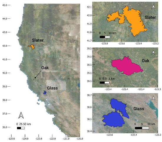
Figure 1.
Location of the fires included in this study (left) and their final perimeters (right). Data source: Cal Fire historical fire perimeters database [28].
Based on visual and histogram inspection, images suitable for analysis were selected by discarding images where fire was not present or that did not contain enough pixels with intensities above background pixels, as well as images where fire pixels filled the entire frame and images with too few fire pixels to contain a distinguishable fire geometry. Examples of images used from the database can be seen in Figure 2. Selected images were converted to 8-bit to accommodate the input requirements of some existing image processing libraries.
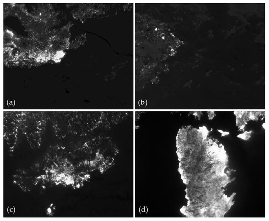
Figure 2.
Four LWIR images captured during the 2020 Oak (a–c) and Glass (d) fires in California, USA. Darker pixels represent areas of low fire intensity or background values, whereas brighter pixels represent more intense areas of the fire. These images provide a good representation of how the fire geometries and fire area intensities can vary.
2.2. Image Processing Background
This section summarizes basic information about the image processing techniques used to build the fire area and fire edge detection methods described in Section 2.3.
2.2.1. Thresholding and Edge Detection
Thresholding is a standard method of image segmentation to isolate objects of interest in an image. Conversely, edge detection techniques are designed to locate object boundaries. Both approaches are advantageous when working with non-radiometric images.
Otsu’s method of binarization [29] is a common segmentation method that analyzes an image’s histogram by minimization of weighted variance to obtain an optimum threshold. Pixel values above that threshold are given one value and pixel values below the threshold are given another (0 and 1 for example). Essentially, Otsu’s method identifies two clearly expressed pixel intensity peaks in the histogram and separates the image into two clusters based on the determined threshold value. Multi-thresholding [30] allows for the identification of multiple threshold values to classify more than two clusters of pixel intensity into brightness regions [31].
After testing multiple edge detection methods, Ref. [20] found the Canny edge detector [32] to outperform other alternatives at identifying active fire fronts, so that method was further explored in this study. The Canny edge detector first applies a Gaussian filter to smooth the image, detects main edges using gradient masks and discards non-edges, then uses upper and lower thresholding values to identify strong edges and weak edges. Strong edges are considered values above the upper thresholding value and weak edges are considered when they lie between the upper and lower thresholds and are connected to strong edges. Values below the lower threshold are discarded.
2.2.2. Morphological Functions
In complex images thresholding and edge detection may exclude pixels required to depict the full object, include pixels outside the object area, and may result in broken or non-continuous edges. This can happen when pixel intensities are similar to those of background pixels. Morphological operators are useful ways of dealing with these discrepancies [18] by providing attribute outputs of active elements inside an image. The erosion operation erodes the outer surface of the foreground object (e.g., the fire area) where the eroded boundary is turned to zero and white noise is discarded. Dilation increases the size of the foreground object increasing the size of the object area. Since erosion and dilation are often performed together in image analysis, a closing feature utilizes both transformations by first applying the dilation operation and then the erosion operation. Filling binary holes is a transformation based on dilation where background pixels of a binary image inside an identified area are connected and changed to foreground pixels until the boundary is reached. Morphological operators can iterate as many times as necessary. Mathematics and detailed descriptors of morphology can be found in Ref. [33].
2.2.3. Structure Analysis
Detecting edges in complex images often results in more than one identified edge. For instance, some of the images available for this study do not have a distinguished flaming zone such as the one that can be observed in laboratory or prescribed burns where only one or two strong gradients between fire pixels and non-fire pixels exist. Instead, multiple strong gradients may exist inside the fire area making it difficult to outline only a single fire edge. This requires unwanted edges to be removed. Structural analysis and shape descriptors compute connected components of an image, assign a label, and produce statistics for each label [34]. Statistics produced for each component are then used to select or discard edges of certain properties.
2.3. Identification of Fire Area and Fire Edges
Identifying fire pixels and the fire area (burning area within the fire perimeter) is challenging because the range of pixel intensities and fire geometry can be highly variable from flight to flight and fire to fire. Low-intensity fire pixel values can be proximal to background pixel intensities and clearly defined maximum intensities are not always present. Furthermore, background pixels (non-fire pixels corresponding to unburned fuels) of similar intensity can reside both inside and outside of the fire area.
When segmenting images, the goal is to distinguish between the fire area and non-fire area. In this work, the fire area is defined as an area that contains either a group of fire pixels or a mixture of fire and background pixels if a cluster of background pixels is within the fire geometry. This definition allows the semi-automated algorithms to be evaluated consistently across all images. Smaller clusters of fire pixels outside the main fire area are also targeted for delineation as they may relate to spotting activity. Active fire edges are considered the perimeter of the main fire area and stand-alone clusters (possible spotting) in each frame.
Several automated thresholding and edge detection methodologies were investigated. Four combined methods were constructed using the canny edge detector, Otsu’s binarization, and thresholding about the mean pixel intensity. Each image was processed individually.
Unless otherwise stated, a Gaussian filter is first applied before thresholding and edge detection for smoothing and noise reduction using a 3 × 3 kernel matrix and a standard deviation determined by the kernel size ( as stated in Equation (1).
2.3.1. Canny Edge Detector
When applying only the canny edge detector to images, variations in lower and upper thresholding values were tested until values of 3 and 7 were determined to provide the best results. Threshold values higher and lower than the selected values excluded pixels considered to belong to the active fire edge, or extensively over-edged fire pixels including pixels belonging to the background. The size of the Sobel kernel used to find the image gradients in the canny operator was set to 3. A closing operation was then performed with a 5 × 5 matrix followed by a binary filling operation to connect non-continuous edges. The canny edge detector was then reapplied a second time after the closing operation with different lower and upper threshold values of 0.3 and 0.7. Edge components under 200 pixels in size were removed using connected component statistics to provide only the active fire edge.
2.3.2. OTSU’s Binarization Followed by Canny Edge Detector
Upon inspection of various fire image histograms and their intensity peaks, Otsu’s method was applied in three ways to deal with the heterogeneity and inconsistencies of the histograms. First, Otsu’s thresholding was applied without any manipulation of the histogram; the second variation applied histogram equalizing and then Otsu’s binarization; and the third variation applied histogram stretching followed by Otsu’s binarization. Following Otsu thresholding, the canny edge detector was applied to characterize the active fire edge. Upper and lower thresholding values used in the canny operator were found to hold any value < 4.4 where the lower threshold value is less than the upper threshold value. Connected component stats were used to remove unwanted edges smaller than 200 pixels. It was found that while histogram stretching and equalization improved the performance of Otsu’s method in some images, it declined performance in other images and, therefore did not enhance the overall results. Because of this, the analysis was carried out using Otsu’s method without any histogram manipulation.
2.3.3. Multi-Thresholding Followed by Canny Edge Detector
Marginal differences between low-intensity fire pixels and background pixels, as well as distinguishing between which background pixels to include in the fire area, is a challenge when only a single threshold value is applied. Therefore, multi-thresholding based on Otsu statistics may be a more robust method. This would allow for classifying different pixel clusters as background pixels, low-intensity pixels, medium-intensity pixels, and high-intensity pixels to be characterized. The rationale behind this approach is that if pixel values could be segmented into multiple clusters of varying intensities, then values could be separated into background pixels that should be included in the fire area and those that should not, pixels of lower fire intensity, and pixels of higher fire intensity. Groups of clusters can then be merged to provide a more accurate representation of the fire area. To investigate this hypothesis, multi-Otsu thresholding operations were performed with four and five classes. Each class was identified as a single region, and regions containing the wanted clusters of pixels were combined. Canny edge detection was then used with the same structure as when applying Otsu’s method. Unwanted edges under 125 pixels in size were removed.
Thresholding by four classes segmented pixel values into two sets of background pixels and two sets of fire pixels, essentially providing a set of background pixels and a set of fire pixels. This fails to provide a classification for those pixels on the border of being background or fire, therefore it was determined that using five classes was ideal to achieve the desired outcome. However, the processing time of segmenting a single image significantly increased when expanding from four classes to five classes, deeming the five-class method impractical for processing large datasets, so the method was tested using four classes. Computational time when setting four classes and processing 100 images from different fires took a total time of 25.49 min yielding an average computation time of 15.29 s per image and a throughput of 0.07 images per second. When increasing the number of classes to five, the algorithm was left to run for one hour before halting the process, where the algorithm had not yet completed four images. This test was performed using an ROG Zephyrus laptop with an AMD Ryzen 9 processor and 32.0 GB of RAM.
2.3.4. Alternate Intensity Thresholding
Here, we introduce the fourth proposed method, which combines an automated thresholding method with canny edge detection. Following a visual analysis of 21 diverse image histograms from separate flights and fires, two attempts were made at identifying an optimum threshold using intensity values:
where THp is the threshold value, minp and maxp are the minimum and maximum pixel value in each image, pvalues are the pixel values, npixels is the number of pixels in an image, and b is a parameter. Of Equations (2) and (3), Equation (3) produced the best results so it was selected for analysis. Different values of b were investigated until the highest performance value of b = 1.015 was selected based on visual inspection.
The threshold mask from Equation (3) was applied to the Gaussian smoothed image. Afterwards, two filling functions were used to fill the fire area followed by two iterations of dilation and another filling operation. This ensures there is only a single edge inside the fire area when edge detection is applied, otherwise multiple edges may be detected. Erosion was then applied to reduce any part of the fire area that protruded from the perimeter or any rogue non-fire pixels scattered throughout the frame. Dilation and erosion transformations were applied using a 5 × 5 matrix. Finally, canny edge detection was performed with an upper threshold value of 4.4 and a lower threshold of any value < 4.4. Edges smaller than 250 pixels were removed. Multiple sequences of the morphological operations were tested where the operations were interchanged. Other sequences failed to provide satisfactory results because they either left holes inside the segmented images that were distinguished as false edges, created edges extending beyond the active fire perimeter, or maintained non-continuous points along the fire edge. Figure 3 illustrates the results after each processing step, which include thresholding according to Equation (3), morphological operators, and canny edge detection. It can be seen in Figure 3b that morphological operations are necessary to transition from discrete active fire edges around the fire area to a continuous edge more adequate for running edge detection. The final output image provides a sharp continuous line around the active fire edge.
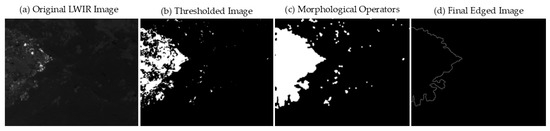
Figure 3.
Progression of the processes involved in contouring active fire edges. (a) Original LWIR image; (b) output of applying the threshold mask utilizing Equation (3), (c) output of the threshold mask after applying morphological operations, and (d) final output when applying the canny edge detector and removing unwanted edges. The threshold image shown in (b) provides a good example of why morphological operations are necessary after applying a threshold mask given the gaps along the edge of the fire area. Looking at (c), gaps in the active fire edge and area have diminished leaving a more continuous edge to be contoured.
Figure 4 shows a block diagram outlining the various processes used in the four methods for identifying the fire area and active fire fronts.
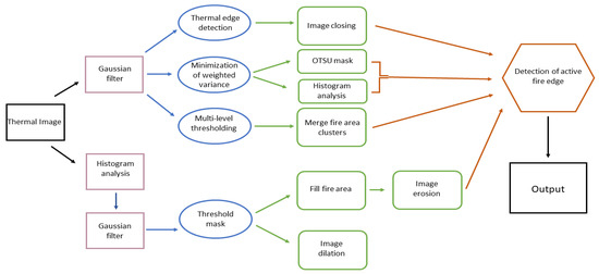
Figure 4.
Block diagram showing the order of operations for the four automated methods tested (canny edge detection, OTSU’s binarization, multi-thresholding, and thresholding about the mean pixel intensity). Black boxes represent the input and output; purple boxes indicate the initial step for each method; blue ovals are the main thresholding or edge detection algorithm used; green soft rectangles are secondary analysis tools, such as morphological operators; and the orange hectogon signifies the final step of detecting the active fire edge.
2.4. Polygonization for Quality Assessment
In order to compare the results of the designed algorithm against manually delineated fire edges, each group of edged raster pixels was vectorized into polygons by utilizing the GDAL polygonize function, version 3.7.0. GDAL software is a translator library for raster and vector geospatial data formats [35], and the polygonize function creates vector polygons for connected regions of pixels in a raster sharing a common pixel value. By translating the edged pixels into polygons, comparisons can then be made between the automated polygon and ground truth polygon. Due to transformations between raster types and polygons, not all active fire edges were converted to be continuous, therefore dilation was necessary. In more complex mosaics, only applying the polygonize function and dilation was insufficient because the fire edge still lacked continuity, unable to render a single polygon. In those cases, an alpha shape function (a concave geometry enclosing vertices) was used to produce a continuous polygon. An alpha value of 0.015 was applied and holes created by the concave hull within the edge polygon were eliminated. For Oak Flight 3, several minuscule holes persisted in the polygon and therefore were closed manually without any new digitization. It is worth noting that the need for extra processes is caused by the conversion from raster to vector layers and not produced by the edge detection algorithm. The use of the polygonize function and alpha shapes allow for the creation of single polygons of the edged mosaics in order to assess error metrics in the semi-automated method.
3. Results
3.1. Method Comparison
Individually applying either the canny edge detector, Otsu’s binarization, or multi-thresholding produced highly variable results, working well in some cases when the fire area and geometry were clearly defined yet failing to produce satisfactory results in more complex images. In some cases, the algorithms also failed to produce satisfactory results in simple shapes with a clearly defined fire area. Furthermore, adjustments required to achieve satisfactory results varied across scenarios, i.e., while one adjustment worked well for some of the images, detail was either lost or excessive in other images. Results also varied when the methods were applied to images acquired under different flight and atmospheric conditions. In most instances, other image processing methods (such as morphological operations) would have made no reasonable change in the overall performance of the algorithm. Therefore, it was difficult to achieve generic thresholding parameters that worked successfully for the majority of images.
Due to the difficulty to find consistent generic thresholds, the canny edge detector either over-edged images producing unwanted edges belonging to background pixels, missed edges belonging to the active fire edge, or excessively edged the fire area. This behavior was expected given the complexity of the images, especially where there is a high intermixing of fire and background pixels inside the fire area.
Non-homogeneity in image histograms and non-uniformity in histogram peaks also posed challenges for the Otsu algorithm to consistently threshold the entire fire area. Images where fire intensity was lower had two peaks closer together and proximal to the background pixels. Images where there was a larger number of high fire intensity pixels had a second peak at or near the maximum pixel value giving a higher degree of separation between the two peaks used to calculate the threshold value. Consequently, only pixels with values belonging to the most intense portions of the fire were thresholded. Overall, Otsu’s method worked well for identifying high-intensity areas of the fire in an image but performed poorly in thresholding the entire fire area within the image and it was thus ineffective in allowing the identification of the entire active fire edge.
Multi-thresholding successfully classified the images into four pixel intensity clusters that could be combined into regions of interest and produced better results than single Otsu thresholding. However, the four classes were unable to segment differences between wanted background pixels inside the fire area and unwanted background pixels outside the fire area. Unreasonable processing time when using five classes are a result of the Otsu statistics [31], and future attempts at multi-thresholding might have success implementing other methods.
Automated thresholding conditional to the mean pixel intensity followed by canny edge detection outperformed the other three algorithms by successfully extracting active fire edges over a wide range of image complexity. Not only did the alternate intensity thresholding method in this study contour edges along the main fire perimeter in each frame, but it also contoured smaller clusters of fire pixels separated from the main fire area possibly indicative of spotting. In a few cases, the algorithm outlined edges extending from the fire area, not capturing the full active fire edge, or breaking continuous segments into multiple edges. As expected, these mostly occur where no clear active fire edge is visible, fire pixels are speckled throughout the image, or where there are high mixtures of fire and background pixels.
A visual comparison of the segmentation results produced by each tested technique is presented in Figure 5, where each method was manually optimized to provide the best outcome.
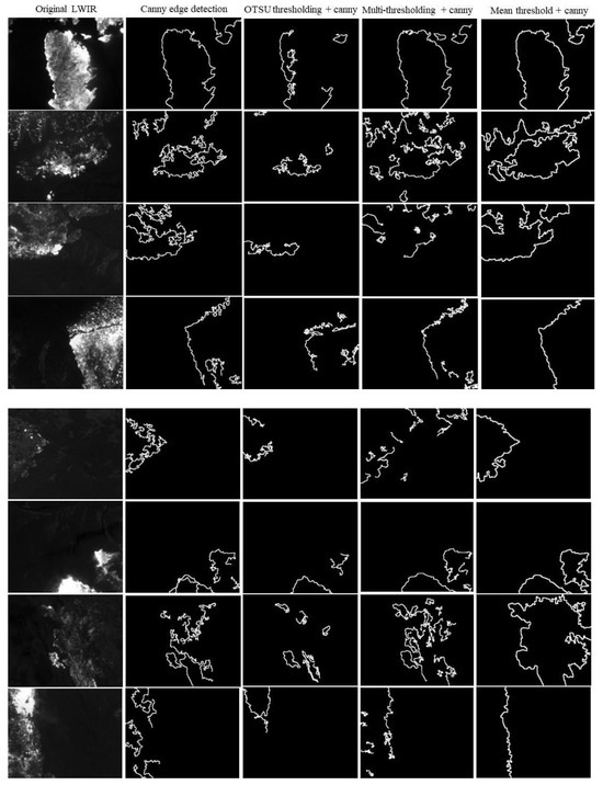
Figure 5.
Four proposed methods of extracting active fire edges are compared against each other. The original LWIR images to which they are applied are shown in the first column. There is a clear distinction between the performance of the fourth method compared to the other three. Mean threshold plus canny edge detection is able to capture active fire edges throughout the diverse fire intensities and geometries.
Based on these results, the alternate intensity thresholding method was selected for implementation in a semi-automated fire edge detection algorithm where automated edges were compared to manually annotated edges and performance metrics were computed. Nonetheless, there were cases where the alternate intensity thresholding method did not provide the expected results. An example is shown in Figure 6.
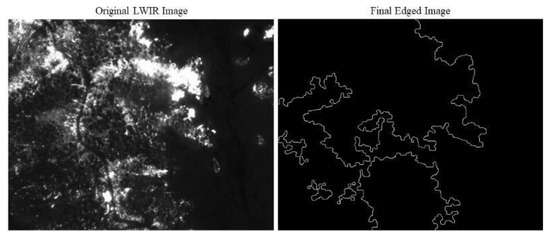
Figure 6.
The original image (left) shows a distinct active fire edge extending from the top of the frame to the bottom of the frame, with a few spotting fire pixels along the right border. After the mean threshold with canny edge detection is applied (right), the method does not delineate the continuous active fire edge but it rather follows gaps in the higher-intensity regions, not accounting for edges mixed with lower-intensity areas.
3.2. Semi-Automated Fire Edge Detection Algorithm
After the comparative analysis presented in Section 3.1, the alternate intensity thresholding method (Section 2.3.4) was selected and implemented in a semi-automated fire edge detection algorithm. This semi-automated algorithm was first applied to individual LWIR images, resulting in binary raster images containing the fire edge and non-fire edge pixels. Individual edge images were then georeferenced and stitched together to generate a mosaic of the entire fire edge as seen in Figure 7. LWIR images were pre-filtered such that if their maximum pixel value did not meet the threshold to be considered a fire pixel, the image was excluded when creating the mosaic. This filtering allowed mosaics to be created only from images containing fire.
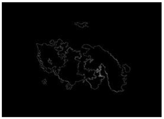
Figure 7.
Reconstruction of the fire edge observed during a flight over the 2020 Oak fire, based on the application of the automated method to individual georeferenced LWIR images and the stitching of edge images into a mosaic. When applied to individual images, the algorithm characterizes more detail in the shape of the active fire edge but is prone to segmenting the main fire area into multiple fire areas.
Figure 7 shows detailed edges around the active fire perimeter as well as spot fires. However, the algorithm also marked as fire a few isolated regions away from the main fire area and a curl extending from the southern side of the main fire geometry even though they actually belong to the background. Furthermore, double edging occurred in some areas. It is hypothesized that double edging is a result of inconsistent edging between concatenated images. Even though an active fire edge may be contoured correctly in one image, differences in pixel intensity and fire geometry across concatenated images may create inconsistencies in the resulting edges. Classification of background pixels as fire pixels outside the active fire edge results from the difficulty in defining a threshold value that distinguishes between background pixels belonging to the fire area and not belonging to the fire area.
The discrepancy in overlapping edges was solved by applying the semi-automated edge algorithm to georeferenced mosaics as displayed in Figure 8. Image mosaics of the original LWIR georeferenced images were created in the open-source GIS platform QGIS for flights of selected fires. Four flights were then selected for evaluation: three flights during the Oak Fire and one flight during the Slater Fire. Flights were selected based on the continuous structure of the active fire edge, which permits a more robust analysis.
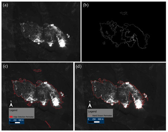
Figure 8.
(a) Mosaic of a single flight taken during the Oak fire (flight 0533), (b) mosaic built after applying the automated algorithm to individual frames, (c) result of applying the automated algorithm to a flight mosaic, and (d) flight mosaic manually annotated active fire edge. When applied to the mosaic (c) a single continuous polygon is created in the main fire area and the double edging effect is diminished.
Figure 8 shows an application example to a flight georeferenced mosaic during the Oak Fire and provides a notion of the image complexity and how fire geometry and intermixing of pixel intensities present a challenging structure for the algorithm. By applying the algorithm to mosaics, the spatial reference information is retained. This change in processing order removed the edges detected within the active fire perimeter (seen in Figure 8b). Several noticeable disparities exist between applying the algorithm to individual images versus a flight mosaic. When applied to the mosaic (Figure 8c), the main fire area becomes a single continuous polygon more similar to the manually annotated mosaic (Figure 8d), whereas applying the method to individual images produces a sharper edge yet neglects faint intensities often cutting inside the fire geometry to follow more distinct intensity gradients (Figure 8b). Meanwhile, when applied to individual georeferenced images the edge is not only sharper around the active fire perimeter but it also distinguishes between fire and smoke. On the contrary, fire perimeters estimated by applying the algorithm to flight mosaics occasionally include smoke. For example, Figure 8c shows how the contoured line follows a thin layer of smoke that extends from the fire edge on the southeast region of the fire geometry, increasing the estimated area of the fire.
Overall, the semi-automated algorithm displayed better performance when applied to flight mosaics instead of individual images, so error metrics were calculated for flight mosaic products. Manually annotated vertices were drawn around the main active fire edge for each of the selected flight mosaics to enclose a single fire area governing as ground truth. Similarity metrics were then computed between the manual ground truth and each of the two georeferencing edged applications: when the delineated active fire edges were polygonized, or when the polygonize function alone was insufficient and polygons were created with the use of concave hull.
Figure 9 shows a comparison between the semi-automated edge detection method applied to image mosaics, the resulting concave hull polygon, and the manually annotated fire perimeter for the four analyzed flights. Generally good agreement can be observed between the automated method and manual annotations of the main fire geometry in Figure 9a,b,d, and a poorer agreement in Figure 9c. The automated method visually performed best for the Slater fire flight (Figure 9d). With the use of the polygonize or concave hull, the active fire edge provides a smoother active perimeter compared to the hand-drawn perimeter, but still captures the fire geometry (shape and size). Over areas of higher fire intensity where the gradient is stronger, the automated and manual edges are analogous, but in areas where small fingers of fire extend from the fire area, and areas where smoke is present, they have shown to be problematic.
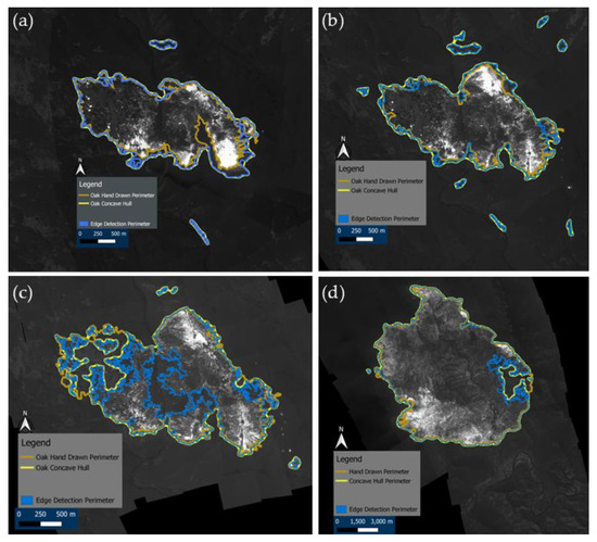
Figure 9.
The four flights used in evaluation metrics: (a) the Oak fire flight 0533, (b) Oak fire flight 0535, (c) Oak fire flight 0537, and (d) Slater fire flight 0553. Each image provides a visualization of the automated method applications. The blue dotted line represents the results of applying the automated method directly to mosaics, the yellow line is after applying the concave hull, and the brown line depicts the hand-drawn annotation.
3.3. Performance Metrics
Five evaluation criteria were used to measure the performance of the semi-automated algorithm: Figure of Merit (FOM) [36] and Baddeley distance [37] were used to assess the similarity of lines produced by the automated edging method and ground truth digitization; the Jaccard index [38] was calculated to measure similarity between the intersection and union of the two sets; the spatial difference in area provided a ratio of the automated area to the manually annotated area; and the difference in areas between the automated and manual polygons was used as an absolute estimation of the error.
FOM and Baddeley distance are common statistical evaluations that have been found useful in assessing wildfire image processing performance, and were computed following the methods of Ref. [20]. FOM characterizes the accuracy of one method against another by inspecting dislocated pixels with a dimensionless output value between 0 and 1, where a value of 1 is the best achievable value. The Baddeley distance is a metric in meters designed to measure the distance between vertices along the automated edge and the manually annotated edged. FOM and Baddeley distance are calculated as follows:
where I is the segmentation result, Igt the corresponding ground truth (hand drawn polygon), card() is the cardinality of the curve (the number of points in the curve), and d(k, Igt) is the minimum distance between point k and curve Igt. α is a constant that takes the value 1/9 as recommended by [36].
The Jaccard index, another common statistical evaluation, was also selected because of its simplicity and universal ability to compare the similarity between two finite sets, and is expressed [39]:
where A and B are two sets, or polygons. Their intersection, , is the region shared by both polygons, and their union, , is the total area that either polygon covers. Jaccard index values range from 0 to 1 where 1 indicates the two sets are identical.
Normalized area differences provide a non-dimensional similarity metric between the automated active fire edge and ground truth annotations, which can also provide insight as to whether the algorithm more commonly under-edges or over-edges. Outer differencing includes the areas where the automated active fire edge detection overextended the fire edge compared to the manually drawn edge, and inner differencing is where the automated detection contoured the edge inside of the manually drawn perimeter. The difference in area of the automated edge detection polygon falling outside and inside the hand-drawn polygon was divided by the total area of the hand-drawn polygon to produce the outer and inner error, respectively, calculated as follows:
where is the normalized area difference, AF is the total area of the automated active fire edge polygon, and AM is the total area of the manually drawn polygon. A value of 0 indicates no difference between the two polygons.
When calculating FOM and Baddeley distance metrics, only the main body of the fire area was taken into consideration, neglecting the smaller false detections by the automated algorithm. For these calculations, we are interested in how accurately the automated polygon was detected compared to a manually annotated polygon. The reason for this is that the FOM and Baddeley metrics are comparing displaced pixels and distances in relation to the manual polygon, so false positives give unreasonable performance errors, making the values more difficult to interpret. Jaccard index, inner and outer differencing, and area comparisons were all made using both correct and incorrect detections of the fire area. Table 1, Table 2 and Table 3 include metric values of the error indices for the statistics calculated in each case of the selected flights.

Table 1.
Evaluation metrics used to assess the performance of the automated method when polygons were created using the gdal polygonize function.
Table 2.
Evaluation metrics used to assess the performance of the automated method when polygons were created using a concave hull.
Table 3.
Area enclosed by hand-drawn and automated fire polygons for each test dataset.
FOM values were close to zero for both the polygonized and concave hull applications with average values of 0.056 and 0.078. These values would normally imply poor performance by the automated method. However, FOM is influenced by the overall size of the polygons, and until now had only been applied to laboratory or experimental fires [4,20]. When working at the landscape scale with mosaic images, fire areas and polygon size are much larger compromising the performance of FOM as an evaluating metric.
Baddeley distances ranged between 14.32 m for Oak Flight 2 and 167,510 m for Oak Flight 3, with an average value of 41,906 m when using the polygonize function and 36.174 m when using the concave hull function. These values are within an expected range, but as with FOM the Baddeley distance is also affected by the overall scale of the polygons, so as the scale in size of the polygons increases the Baddeley distance and FOM metrics will naturally increase as well.
Inner and outer difference values were all closer to zero with a maximum value of 0.322 when the polygonize function was used for Oak Flight 3. Average values for the inner and outer difference when mosaics are polygonized are 0.098 and 0.080 with a total (inner plus outer) average difference of 0.179. Average values for the inner and out difference when the concave hull is applied are 0.041 and 0.135 with a total average difference of 0.176. Values for differencing undergo a behavior opposite that of the Baddeley distance in that as the area of the true polygon increases, the inner and outer differences are divided by a larger number so the error will decrease as scale increases. Figure 10 provides an illustration of inner and outer differencing for the flight during the Slater Fire (flight 0553). One prominent differencing error in blue (inner difference) can be seen where few fire pixels continue the active perimeter and the automated method cuts inside the fire area, but the majority of differencing errors are minor.
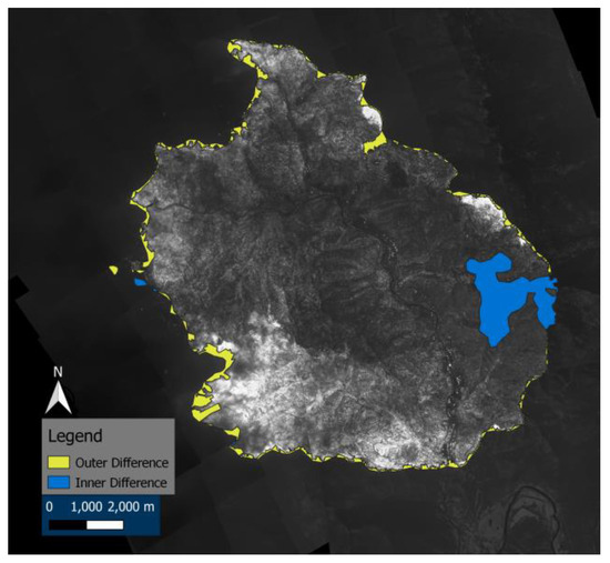
Figure 10.
Area differencing between the automated edged delineation and manual annotation delineation of the active fire edge. Areas shaded in yellow are the outer difference between the automated and manual methods, and blue shading shows inner differences.
Jaccard index values were all above 0.7 ranging from 0.725 to 0.928. Average Jaccard indexes were similar between the polygonize function (0.832), and the application of the concave hull (0.838). The high Jaccard index values indicate that the regions inside the automated polygon are also mostly inside the manually drawn polygon and the two polygons are very similar, which is in alignment with the qualitative visual comparison shown in Figure 9. Several visual characteristics in the active fire perimeter images influence the resulting Jaccard Index values. The Slater fire yields the highest Jaccard Index scores (0.9177 and 0.9284) because its active fire perimeter is smooth and well-defined, with a clear contrast between the fire perimeter and non-fire background. This minimizes ambiguous pixels along the edge. In some Oak Fire datasets (e.g., Oak flight 3 polygonize score of 0.7253 and Oak flight 1 concave hull score of 0.7771), the active fire edge becomes highly irregular in some regions. Complex perimeter shapes create mismatches between the two polygons and smoke protruding from the fire into the background introduces false edges into the fire edge shape.
Simulated burn area is often compared to true burn area in assessing the performance of fire behavior models [40], and when initiating a model run from infrared polygons [41,42], it is important to understand the accuracy of the polygon dimensions. For this, we assess the differences in area by subtracting the area of the automated polygon by that of the ground truth polygon. The largest difference occurred for the Slater flight which underestimated the active fire area by 3,265,051 m2, and the smallest difference was Oak Flight 3 which underestimated the area by 249,116 m2. Concave hull produced the highest difference in area for Oak Flight 1 over-estimating the active fire area by 533,939 m2, and the lowest difference in area occurred for Oak Flight 3 under-estimating the area by 129,149 m2. Average differences in area when polygonized were approximately 1,058,549 m2, and approximately 332,551 m2 when a concave hull was used.
In terms of computing requirements, running the automated algorithm on 2016 images from different fires took 87.94 s, which yields an average computation time of 0.04 s per image and a throughput of 22.92 images per second. This test was performed using a ROG Zephyrus laptop with an AMD Ryzen 9 processor and 32.0 GB of RAM.
4. Discussion
The semi-automated method performed more comparable to ground truth delineations when applied to georeferenced flight mosaics versus georeferenced individual images. Use of the polygonize function and alpha shapes allowed for the creation of single polygons of the edged mosaics to assess error metrics in the automated method by calculating FOM, Baddeley distances, the Jaccard index, a normalized area difference ratio, and differences in polygon areas. FOM values showed poor similarity metrics between the automated and manual method, and while Baddeley distance values were in an expected range, it should be noted that FOM and Baddeley distance are affected by the overall size of the polygons, and may not be appropriate in landscape scale fire delineation analysis. The conversion from 16-bit to 8-bit images simplified algorithm implementation and we did not observe any noticeable information loss due to this conversion. Nonetheless, the change in bit depth entails a theoretical loss of detail that could become significant in images with faint gradients or large dynamic ranges.
It is worth noting that, while the proposed method works well for these case studies and the core of the algorithm is highly generalizable, it is likely some parameters will need to be adjusted when working with other fires or datasets. As described in Section 2.3, the length of edges that need to be removed will vary depending on which processing method is used and which flight is being processed. Similarly, automated threshold values may fluctuate for different fires, and small changes in the value of b in Equation (3) can produce under or over-thresholding. Iterations of morphological functions such as dilation and hole filling will also likely need to be adjusted for different fires. For example, actively burning fires with a well-defined continuous active edge and less geometrically complex will require fewer iterations of dilation or filling, and homogeneity in image histograms between sets of images will provide insight into adjusting threshold values. Similarly, the use of different sensors and image acquisition strategies may also require adjustments to the method and its parameters.
Typically, within laboratory and field experiments, fire spread takes on an elliptical form, providing a simpler shape to segment and contour; however, the heterogeneous fire geometry at the landscape scale can enhance the difficulty in constructing active fire edge algorithms. Although, should this type of data be used to improve fine-scale fire behavior modeling, it may be acceptable to provide polygons of an active fire edge that do not precisely follow a detailed cut-out of the perimeter, but rather a smoothened version of the polygon like the one provided when applying the concave hull in Figure 10.
Errors produced by the automated algorithm such as false positives (over-edging the true perimeter) and false negatives (missed portions of the fire edge) can be linked to environmental and imaging conditions of the dataset. Under windy conditions and in steep terrains, flames, hot gases, and smoke layers may extend beyond the physical fire edge and register as high-intensity pixels causing the algorithm to overestimate the fire perimeter and produce false positives. Low-intensity flaming and smoldering reduces thermal contrast and pixel intensity values that blend with background values and display as a non-continuous active fire edge causing false negatives. Dense vegetation and canopy cover can occlude portions of the flaming edge causing missed portions of the active perimeter and false negatives. In addition, when sensor pixels saturate, local pixel gradients flatten at that intensity point and can mask the true active fireline causing false negatives. Vegetation density influences burning patchiness. In areas where vegetation continuity is lower, multiple gradients within the active fire perimeter may be observed resulting in edges that cut inside the fire polygon.
5. Conclusions
Remote sensing techniques used to monitor and observe wildfires are a critical component of understanding fire dynamics. Their versatility provides means of assessing active fire scenarios from various platforms. However, acquiring and processing the needed observations to improve fire spread calculations is challenging. The datasets used here, while lacking radiometric temperatures of fire, have an extensive number of images that provide value to develop fire spread forecasting models. Semi-automated methods of image processing for extracting active fire edges from tactical infrared imagery were evaluated and compared. A new method proposed in this research, thresholding about the mean pixel intensity plus canny edge detection, outperformed several other common thresholding and edge detection algorithms. The new method provided satisfactory delineation of active fire edges over a range of image complexity belonging to multiple fires.
These results set a foundation for the use of infrared fire observations captured during firefighting operations in fire spread analysis to be applied for research applications. This allows for the evaluation of higher-resolution fire spread dynamics during bouts of extreme fire behavior at the landscape scale, which will in turn serve to develop and advance fine-scale fire behavior models. Our results also reiterate the need for improved methods of extracting high-resolution active fire perimeters from airborne infrared imagery. As future research campaigns focus on taking infrared measurements during landscape wildfires, enhanced automated methods capable of handling large amounts of data are going to be necessary.
Future work will include improving these image processing methods for landscape scale fires observed using high-quality airborne sensors where radiometric data is available. Identifying a threshold capable of identifying background pixels belonging to the fire geometry and those not belonging to the fire geometry will continue to be a difficult task in working with datasets of this size.
Author Contributions
Conceptualization, C.C.G. and M.M.V.; methodology, C.C.G. and E.G.-D.; software, C.C.G., E.G.-D. and A.K.; validation, C.C.G., E.G.-D. and M.M.V.; formal analysis, C.C.G., E.G.-D. and M.M.V.; investigation, C.C.G. and E.G.-D.; resources, M.M.V.; data curation, C.C.G., E.G.-D. and A.K.; writing—original draft preparation, C.C.G. and E.G.-D.; writing—review and editing, C.C.G. and M.M.V.; visualization, C.C.G. and E.G.-D.; supervision, M.M.V.; project administration, M.M.V.; funding acquisition, M.M.V. All authors have read and agreed to the published version of the manuscript.
Funding
This research was funded by the U.S. National Science Foundation under award number 2053619.
Data Availability Statement
The original contributions presented in this study are included in the article. Further inquiries can be directed to the corresponding author(s).
Acknowledgments
We thank CAL FIRE for the data used in this study and for their insights about fire observational capabilities and needs during firefighting operations.
Conflicts of Interest
The author Christopher C. Giesige is employed by the company Telops-Exosens. The remaining author declares that the research was conducted in the absence of any commerical or financial relationships that could be construed as a potential conflict of interest.
Abbreviations
The following abbreviations are used in this manuscript:
| CalFiDE | California Fire Dynamics Experiment |
| CAL FIRE | California Department of Forestry and Fire Protection |
| FOM | Figure of Merit |
| FRP | Fire Radiative Power |
| GIS | Geographic Information System |
| LTM | Landsat Thematic Mapper |
| LWIR | Long-Wave Infrared |
| MODIS | Moderate Resolution Infrared Sensor |
| NDBR | Normalized Difference Burn Ratio |
| NDVI | Normalized Difference Vegetation Index |
| ROS | Rate of Spread |
| RxCADRE | Prescribed Fire Combustion and Atmospheric Dynamics Research Experiment |
References
- Duane, A.; Castellnou, M.; Brotons, L. Towards a comprehensive look at global drivers of novel extreme wildfire events. Clim. Change 2021, 165, 43. [Google Scholar] [CrossRef]
- Hantson, S.; Andela, N.; Goulden, M.L.; Randerson, J.T. Human-ignited fires result in more extreme fire behavior and ecosystem impacts. Nat. Commun. 2022, 13, 2717. [Google Scholar] [CrossRef]
- Stephens, S.L.; Weise, D.R.; Fry, D.L.; Keiffer, R.J.; Dawson, J.; Koo, E.; Potts, J.; Pagni, P.J. Measuring the rate of spread of chaparral prescribed fires in Northern California. Fire Ecol. 2008, 4, 74–86. [Google Scholar] [CrossRef]
- Rudz, R.; Chetehouna, K.; Sèro-Guillaume, O.; Pastor, E.; Planas, E. Comparison of two methods for estimating fire positions and the rate of spread of linear flame fronts. Meas. Sci. Technol. 2009, 20, 115501. [Google Scholar] [CrossRef]
- Loboda, T.V.; Csiszar, I.A. Reconstruction of fire spread within wildland fire events in Northern Eurasia from the MODIS active fire product. Glob. Planet. Change 2007, 65, 258–273. [Google Scholar] [CrossRef]
- Viedma, O.; Quesada, J.; Torres, I.; De Santis, A.; Moreno, J.M. Fire severity in a large fire in a Pinus pinaster forest is highly predictable from burning conditions, stand structure, and topography. Ecosystems 2015, 18, 237–250. [Google Scholar] [CrossRef]
- Rudz, S.; Chetehouna, K.; Hafiane, A.; Laurent, H.; Sèro-Guillaume, O. Investigation of a novel image segmentation method dedicated to forest fire applications. Meas. Sci. Technol. 2013, 24, 75403. [Google Scholar] [CrossRef]
- Toulouse, T.; Rossi, L.; Celik, T.; Akhloufi, M. Automatic fire pixel detection using image processing: A comparative analysis of rule-based and machine learning-based methods. SIViP 2016, 10, 647–654. [Google Scholar] [CrossRef]
- Wooster, M.J.; Roberts, G.; Smith, A.M.S.; Johnston, J.; Freeborn, P.; Amici, S.; Hudak, A.T. Thermal infrared remote sensing: Sensors, methods, applications. In Remote Sensing and Digital Image Processing; Kuenzer, C., Dech, S., Eds.; Springer International Publishing: Berlin/Heidelberg, Germany, 2013; pp. 347–390. [Google Scholar]
- O’Brien, J.J.; Loudermilk, E.L.; Hornsby, B.; Hudak, A.T.; Bright, B.C.; Dickinson, M.B.; Hiers, J.K.; Teske, C.; Ottmar, R.D. High-resolution infrared thermography for capturing wildland fire behaviour-RxCADRE. Int. J. Wildland Fire 2016, 25, 62–75. [Google Scholar] [CrossRef]
- Wooster, M.J.; Roberts, G.; Perry, G.L.W. Retrieval of biomass combustion rates and totals from fire radiative power observations: FRP derivation and calibration relationships between biomass consumption and fire radiative energy release. J. Geophys. Res. 2005, 110, D24311. [Google Scholar] [CrossRef]
- Riggan, P.J.; Tissell, R.G. Developments in Environmental Science; Elsevier B.V.: Amsterdam, The Netherlands, 2009; Volume 8. [Google Scholar]
- Paugam, R.; Wooster, M.J.; Roberts, G. Use of handheld thermal imager data for airborne mapping of fire radiative power and energy and flame front rate of spread. IEEE Trans. Geosci. Remote Sens. 2013, 51, 3385–3399. [Google Scholar] [CrossRef]
- Stow, D.A.; Riggan, P.J.; Storey, E.J.; Coulter, L.L. Measuring fire spread rates from repeat pass airborne thermal infrared imagery. Remote Sens. Lett. 2014, 5, 803–812. [Google Scholar] [CrossRef]
- Pastor, E.; Àgueda, A.; Andrade-Cetto, J.; Muñoz, M.; Pérez, Y.; Planas, E. Computing the rate of spread of linear flame fronts by thermal image processing. Fire Saf. J. 2006, 41, 569–579. [Google Scholar] [CrossRef]
- Martìnez-de Dios, J.R.; Merino, L.; Caballero, F.; Ollero, A. Automatic forest-fire measuring using ground stations and unmanned aerial systems. Sensors 2011, 11, 6328–6353. [Google Scholar] [CrossRef]
- Johnston, J.M.; Wooster, M.J.; Paugam, R.; Wang, X.; Lynham, T.J.; Johnston, L.M. Direct estimation of Byram’s fire intensity from infrared remote sensing imagery. Int. J. Wildland Fire 2017, 26, 668–684. [Google Scholar] [CrossRef]
- Ononye, A.E.; Vodacek, A.; Saber, E. Automated extraction of fire line parameters from multispectral infrared images. Remote Sens. Environ. 2007, 108, 179–188. [Google Scholar] [CrossRef]
- Valero, M.M.; Rios, O.; Mata, C.; Pastor, E.; Planas, E. An integrated approach for tactical monitoring and data-driven spread forecasting of wildfires. Fire Saf. J. 2017, 91, 835–844. [Google Scholar] [CrossRef]
- Valero, M.M.; Rios, O.; Planas, E.; Pastor, E. Automated location of active fire perimeters in aerial infrared imaging using unsupervised edge detectors. Int. J. Wildland Fire 2018, 27, 241–256. [Google Scholar] [CrossRef]
- Stow, D.; Riggan, P.; Schag, G.; Brewer, W.; Tissell, R.; Coen, J.; Storey, E. Assessing uncertainty and demonstrating potential for estimating fire rate of spread at landscape scales based on time sequential airborne thermal infrared imaging. Int. J. Remote Sens. 2019, 40, 4876–4897. [Google Scholar] [CrossRef]
- Schag, G.M.; Stow, D.A.; Riggan, P.J.; Tissell, R.G.; Coen, J.L. Examining landscape-scale fuel and terrain controls of wildfire spread rates using repetitive airborne thermal infrared (ATIR) imagery. Fire 2021, 4, 6. [Google Scholar] [CrossRef]
- Clements, C.B.; Davis, B.; Seto, D.; Contezac, J.; Kochansk, A.; Fillipi, J.-B.; Lareau, N.; Barboni, B.; Butler, B.; Krueger, S.; et al. Fire behavior modeling. In Advances in Forest Fire Research; Vieges, D.X., Ed.; Imprensa da Uniersidade de Coimbra: Coimbra, Portugal, 2013; pp. 392–400. [Google Scholar]
- Dickinson, M.B.; Hudak, A.T.; Zajkowski, T.; Loudermilk, E.L.; Schroeder, W.; Ellison, L.; Kremens, R.L.; Holley, W.; Martinez, O.; Paxton, A.; et al. Measuring radiant emissions from entire prescribed fires with ground, airborne and satellite sensors—RxCADRE 2012. Int. J. Wildland Fire 2016, 25, 48–61. [Google Scholar] [CrossRef]
- Hudak, A.T.; Dickinson, M.B.; Bright, B.C.; Kremens, R.L.; Loudermilk, E.L.; O’Brien, J.J.; Hornsby, B.S.; Ottmar, R.D. Measurements relating fire radiative energy density and surface fuel consumption—RxCADRE 2011 and 2012. Int. J. Wildland Fire 2016, 25, 25–37. [Google Scholar] [CrossRef]
- Carroll, B.J.; Brewer, W.A.; Strobach, E.; Lareau, N.; Brown, S.S.; Valero, M.M.; Kochanski, A.; Clements, C.B.; Kahn, R.; Junghenn Noyes, K.T.; et al. Measuring Coupled Fire–Atmosphere Dynamics: The California Fire Dynamics Experiment (CalFiDE). Bull. Am. Meteorol. Soc. 2024, 105, E690–E708. [Google Scholar] [CrossRef]
- Cal Fire. 2020 Fire Season Incident Archive. 2020. Available online: https://www.fire.ca.gov/incidents/2020/ (accessed on 20 October 2025).
- Cal Fire. Historical Fire Perimeters. 2025. Available online: https://www.fire.ca.gov/what-we-do/fire-resource-assessment-program/fire-perimeters (accessed on 20 October 2025).
- Otsu, N. A threshold selection method from gray-level histograms. IEEE Trans. Syst. Man Cybern. 1979, SMC-9-1, 62–66. [Google Scholar] [CrossRef]
- Huang, D.; Lin, T.; Hu, W. Automatic multilevel thresholding based on two-stage OTSU’s method with cluster determination by valley estimation. Int. J. Innov. Comput. Inf. Control 2011, 7, 5631–5644. [Google Scholar]
- Arora, S.; Acharya, J.; Verma, A.; Panigrahi, P.K. Multilevel thresholding for image segmentation through a fast statistical recursive algorithm. Pattern Recognit. Lett. 2008, 29, 119–125. [Google Scholar] [CrossRef]
- Canny, J. A computational approach to edge detection. IEEE Trans. Pattern Intell. Mach. Learn. 1986, 6, 679–698. [Google Scholar] [CrossRef]
- Gonzalez, R.C.; Woods, R.E. Digital Image Processing, 2nd ed.; Prentice Hall: Upper Saddle River, NJ, USA, 2002. [Google Scholar]
- Bradski, G. The OpenCV Library. 2000. Available online: https://docs.opencv.org/3.4/d3/dc0/group__imgproc__shape.html (accessed on 20 October 2025).
- GDAL/ORG Contributors. GDAL/ORG Geospatial Data Abstraction software Library. Open Source Geospatial Foundation. 2025. Available online: https://zenodo.org/records/17098582 (accessed on 20 October 2025).
- Pratt, W.K. Digital Image Processing; John Wiley & Sons Inc.: New York, NY, USA, 1991. [Google Scholar]
- Baddeley, A. An error metric for binary images. In Robust Computer Vision: Quality of Vision Algorithms; Förstner, W., Ruwiedel, S., Eds.; Wichmann: Karlsruhe, Germany, 1992; pp. 59–78. [Google Scholar]
- Jaccard, P. Distribution de la flore alpine dans le bassin des dranses et dans quelques r’egions voisines. Bull. Soci’et’e Vaudoise Sci. Nat. 1901, 37, 241–272. [Google Scholar]
- Costa, L.D.F. Further generalizations of the Jaccard index. arXiv 2021, arXiv:2110.09619. [Google Scholar] [CrossRef]
- Monedero, S.; Ramirez, J.; Cardil, A. Predicting fire spread and behavior on the fireline. Wildfire Analyst pocket: A mobile app for wildland fire prediction. Ecol. Model. 2019, 392, 103–107. [Google Scholar] [CrossRef]
- Kochanski, A.K.; Mallia, D.V.; Fearon, M.G.; Mandel, J.; Souri, A.H.; Brown, T. Modeling wildfire smoke feedback mechanisms using a coupled fire-atmosphere model with a radiatively active aerosol scheme. J. Geophys. Res. Atmos. 2019, 124, 9099–9116. [Google Scholar] [CrossRef]
- Kochanski, A.K.; Herron-Thorpe, F.; Mallia, D.V.; Mandel, J.; Vaughan, J.K. Integration of a coupled fire-atmosphere model into a regional air quality forecasting system for wildfire events. Front. For. Glob. Change 2021, 4, 728726. [Google Scholar] [CrossRef]


Disclaimer/Publisher’s Note: The statements, opinions and data contained in all publications are solely those of the individual author(s) and contributor(s) and not of MDPI and/or the editor(s). MDPI and/or the editor(s) disclaim responsibility for any injury to people or property resulting from any ideas, methods, instructions or products referred to in the content. |
© 2025 by the authors. Licensee MDPI, Basel, Switzerland. This article is an open access article distributed under the terms and conditions of the Creative Commons Attribution (CC BY) license (https://creativecommons.org/licenses/by/4.0/).