Article

Spatiotemporal Variations and Seasonal Climatic Driving Factors of Stable Vegetation Phenology Across China over the Past Two Decades

1
College of Resources, Sichuan Agricultural University, Chengdu 611130, China
2
Key Laboratory of Investigation and Monitoring, Protection and Utilization for Cultivated Land Resources, Ministry of Natural Resources, Chengdu 611130, China
*
Author to whom correspondence should be addressed.
Remote Sens. 2025, 17(20), 3467; https://doi.org/10.3390/rs17203467
Submission received: 19 August 2025 / Revised: 12 October 2025 / Accepted: 15 October 2025 / Published: 17 October 2025

Abstract

Highlights

What are the main findings?
  • SIF demonstrates a significantly better performance in extracting vegetation phenology compared to NDVI, EVI, and LAI;
  • Short-term vegetation interference was excluded during the analysis of vegetation phenology’s response to climate change;
What is the implication of the main finding?
  • Latitudinal variation in vegetation phenology is more pronounced than the longitudinal variation;
  • SOS advances more rapidly in climate zones that are located further south and the more humid and warmer; EOS is positively correlated with summer vapor pressure deficit(vpd) and negatively correlated with autumn vpd.

Abstract

Vegetation phenology (VP) is a crucial biological indicator for monitoring terrestrial ecosystems and global climate change. However, VP monitoring using traditional remote sensing vegetation indices has significant limitations in precise analysis. Furthermore, most studies have overlooked the distinction between stable and short-term VP in relation to climate change and have failed to clearly identify the seasonal variation in the impact of climatic factors on stable VP (SVP). This study compared the accuracy of solar-induced chlorophyll fluorescence (SIF) and three traditional vegetation indices (e.g., Normalized Difference Vegetation Index) for estimating SVP in China, using ground-based data for validation. Additionally, this study employs Sen’s slope, the Mann–Kendall (MK) test, and the Hurst index to reveal the spatiotemporal evolution of the Start of Season (SOS), End of Season (EOS), and Length of Growing Season (LOS) over the past two decades. Partial correlation analysis and random forest importance evaluation are used to accurately identify the key climatic drivers of SVP across different climate zones and to assess the seasonal contributions of climate to SVP. The results indicate that (1) phenological metrics derived from SIF data showed the strongest correlation coefficients with ground-based observations, with all correlation coefficients (R) exceeding 0.69 and an average of 0.75. (2) The spatial distribution of SVP in China has revealed three primary spatial patterns: the Tibetan Plateau, and regions north and south of the Qinling–Huaihe Line. From arid, cold-to-warm, and humid regions, the rate of SOS advancement gradually increases; EOS transitions from earlier to nearly unchanged; and the rate of LOS delay increases accordingly. (3) The spring climate primarily drives the advancement of SOS across China, contributing up to 70%, with temperatures generally having a negative effect on SOS (r = −0.53, p < 0.05). In contrast, EOS is regulated and more complex, with the vapor pressure deficit exerting a dual ‘limitation–promotion’ effect in autumn (r = −0.39, p < 0.05) and summer (r = 0.77, p < 0.05). This study contributes to a deeper scientific understanding of the interannual variability in SVP under seasonal climate change.

1. Introduction

Vegetation phenology (VP) refers to the study of the timing of recurring biological events, the biotic and abiotic factors influencing these timings, and the interrelationships among different phenological phases of the same or different species [1]. It reflects plant adaptation to seasonal variations in climate and environmental factors, establishing a growth and development rhythm characterized by an annual cycle. VP is highly sensitive to climate change [2], which is why it is often referred to as the “diagnostic fingerprint” [3] and the “optimal indicator” [4]. Furthermore, VP affects the carbon, water, and energy exchanges between the land and the atmosphere [5], playing a crucial role in advancing the achievement of the “dual carbon” goals and the development of ecological civilization. Therefore, understanding VP responses to seasonal climate changes is crucial for enhancing our understanding of land–atmosphere interactions in a changing climate.
Currently, satellite remote sensing, compared to station-based observations, offers spatially comprehensive VP data for various ecosystems and has become a key method for monitoring VP responses to seasonal climate change [6]. For instance, MODIS data products have been extensively used in VP studies [7,8,9]. However, traditional vegetation indices, such as the Normalized Difference Vegetation Index (NDVI) [10], the Enhanced Vegetation Index (EVI) [11], and the Leaf Area Index (LAI) [12], are influenced by clouds, snow, and bare rock surfaces [13], which complicate the accurate capture of canopy greenness and monitoring of actual photosynthetic changes [14]. Solar Induced Chlorophyll Fluorescence (SIF) provides new possibilities for spatial monitoring of VP [15]. It is the energy flux re-emitted by plants within nanoseconds of absorbing sunlight, and it can directly reflect the dynamic changes in vegetation photosynthesis [16,17,18,19]. Unlike traditional vegetation indices based on reflectance, SIF is more closely linked to photosynthetic activity. Therefore, SIF data offers a promising alternative for more precise VP estimation [20,21]. However, systematic comparative studies using SIF data for phenology estimation in China remains limited.
In recent years, several large-scale studies have estimated VP using SIF. Wang et al. validated phenological periods estimated from NDVI, EVI, and SIF in China, using those derived from Gross Primary Productivity (GPP) as a reference [22]. Zhou et al. analyzed the spatial patterns and trends of VP across the Northern Hemisphere using SIF [23]. However, the spatial resolution of the remote sensing data (0.5 degrees, approximately 50 km) was insufficient to accurately capture the fine-scale spatial details of regional VP periods. Several studies have focused on VP in smaller regions, such as Bao et al.’s investigation of the impacts of climate change and ozone on vegetation SOS and EOS in the Tibetan Plateau of China [24], Zhang et al.’s study on the response of VP to preseason temperature and precipitation in northern China [25], and Ji et al.’s research on variations in vegetation SOS and EOS under different vegetation types in the Loess Plateau [26]. However, although these studies have improved resolution, they primarily reflect the distribution of VP in specific local areas, limiting our understanding of VP changes at larger scales. Moreover, relatively few studies differentiate phenological differences between stable vegetation (e.g., natural forests) and short-term vegetation (e.g., crops) in relation to VP changes and climate. In contrast to short-term vegetation, such as crops, whose phenology is significantly influenced by direct human factors (e.g., planting systems) [27,28,29,30], the phenological changes in vegetation in areas with stable land cover (e.g., natural forests) are thought to more directly reflect responses to climatic and other natural factors, despite potential diffuse anthropogenic influences. Therefore, systematically investigating changes in stable VP (SVP) is of significant scientific importance for revealing the sensitivity of natural ecosystems to climate change.
SVP refers to the phenology observed in areas with stable vegetation cover, where it has remained consistent over a specified period. Changes in SVP are driven by complex interactions between biological and environmental factors [18,31], and significant differences exist in identifying the underlying drivers of these changes. For example, some studies argue that autumn warming is the primary factor driving the delayed trend of EOS in most areas of the Northern Hemisphere’s mid-to-high latitudes [32], while precipitation is the primary driver of delayed EOS in arid and semi-arid regions [33]. Shen et al.’s study indicates that the advancement of SOS is primarily driven by the continued rise in winter temperatures [34] or increased precipitation [35]. Further research indicates that SOS is negatively correlated with temperatures, particularly in March, prior to the season, and positively correlated with precipitation from the previous autumn and winter [36]. Menzel et al. found in their study across 21 European countries that for each 1 °C increase in temperature, the timing of leaf-out advances by 2.5 days, while leaf-fall is delayed by 1 day [37]. Although numerous studies have examined the relationship between VP and climate, most focus primarily on the two major climate factors, temperature and precipitation, while overlooking the influence of other potential drivers, such as soil moisture and vapor pressure deficit. Furthermore, detailed studies on the response of SVP to seasonal climate are lacking [38], and the dominant season affecting SVP remains unclear.
This study aims to address the following three questions: (1) Which of the four remote sensing datasets—NDVI, EVI, LAI, and SIF—yields the highest accuracy in estimating phenological metrics (e.g., SOS)? (2) How has SVP in China evolved spatially and temporally over the past two decades? (3) What is the relationship between the changes in SVP and seasonal climate factors? This study provides new insights into the factors influencing SVP in China and contributes to a deeper understanding of how stable vegetation interacts with seasonal climate variations.

2. Materials and Methods

2.1. Study Area

The geographical extent of China spans approximately from 73°E to 135°E in longitude and from 3°N to 53°N in latitude [39]. China exhibits a wide range of climate types, with significant variations in temperature and humidity, from humid monsoon climates along the southeastern coast to arid climates in the northwest, encompassing tropical, subtropical, and temperate zones. According to Zhao et al.’s research, based on long-term averages of temperature, precipitation, and humidity, China is classified into seven natural zones (Figure 1c) [40]. Furthermore, China is characterized by widespread vegetation cover, with forests primarily distributed in the southeastern and northeastern regions, showing a clear latitudinal zonation from north to south, while grasslands are widespread in the northwest (Figure 1b). The stable vegetation areas consisted primarily of two types of natural ecosystems: grasslands (approximately 72.8%) and forests (approximately 27.2%) (Figure 1).

2.2. Data Sources and Preprocessing

This study utilizes remote sensing datasets spanning from 2003 to 2022, including the Global “OCO-2” SIF (GOSIF) and three MODIS products retrieved from the Google Earth Engine (GEE) cloud platform (Table 1). GOSIF was generated using machine learning algorithms trained on discrete SIF observations from OCO-2 satellite. The machine learning model integrates continuous MODIS EVI data and meteorological variables (air temperature, vapor pressure deficit, and shortwave radiation) from MERRA-2 to produce spatially and temporally continuous SIF estimates [41]. Climate data were obtained from the Terra Climate dataset, which provides monthly climate data and climate water balance information for global land areas. The average values of soil moisture (sm), downward shortwave radiation (srad), precipitation (pr), air temperature (tem), vapor pressure deficit (vpd), and potential evapotranspiration (pet) were calculated by using GEE for winter (December of the previous year to February), spring (March to May), summer (June to August), and autumn (September to November) from 2003 to 2022.
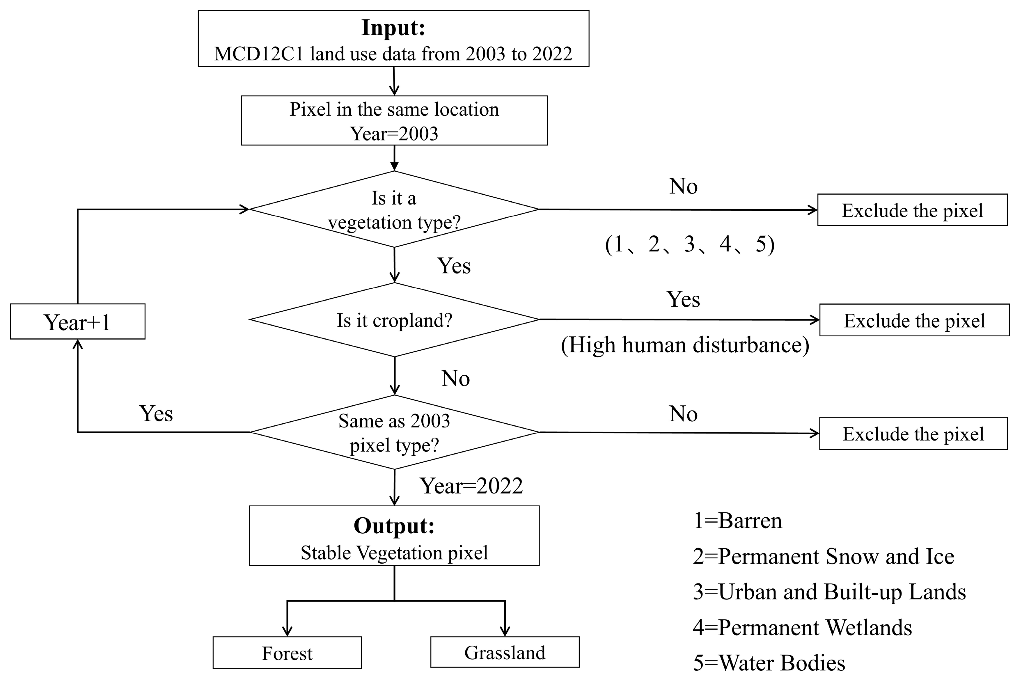
Then, regions in China with unchanged land-use types from 2003 to 2022 were identified. To isolate the long-term signals of climate change from short-term disturbances caused by land use changes and direct human management, this study focuses on “stable vegetation areas”—regions of natural vegetation where land cover types remained unchanged from 2003 to 2022. As shown in Figure 2, we first excluded all non-vegetation land cover types (e.g., Barren, water bodies, and Permanent Wetlands). Secondly, to further reduce the high human disturbance, all croplands were removed. Finally, pixels with changes in vegetation types from 2003 to 2022 were excluded. These classifications were based on MODIS land cover data (Table 1). Bilinear resampling was applied to harmonize the spatial resolution of all datasets to 0.05°.
Final, phenological validation data were obtained from the National Ecosystem Science Data Center, which includes phenological observations from 22 stations during 2003–2015 (Figure 1b), such as Gongga Mountain, Maoxian, Puding, Ailao Mountain, and Changbai Mountain. The dataset was divided into a woody subset and a herbaceous subset, the green-up and senescence dates of grasslands at the 22 ground observation stations were matched to the leaf-out and leaf-fall dates of forests, respectively, and their averages were calculated to define the vegetation SOS and EOS, thereby improving the comparability of the validation data.

2.3. Methods

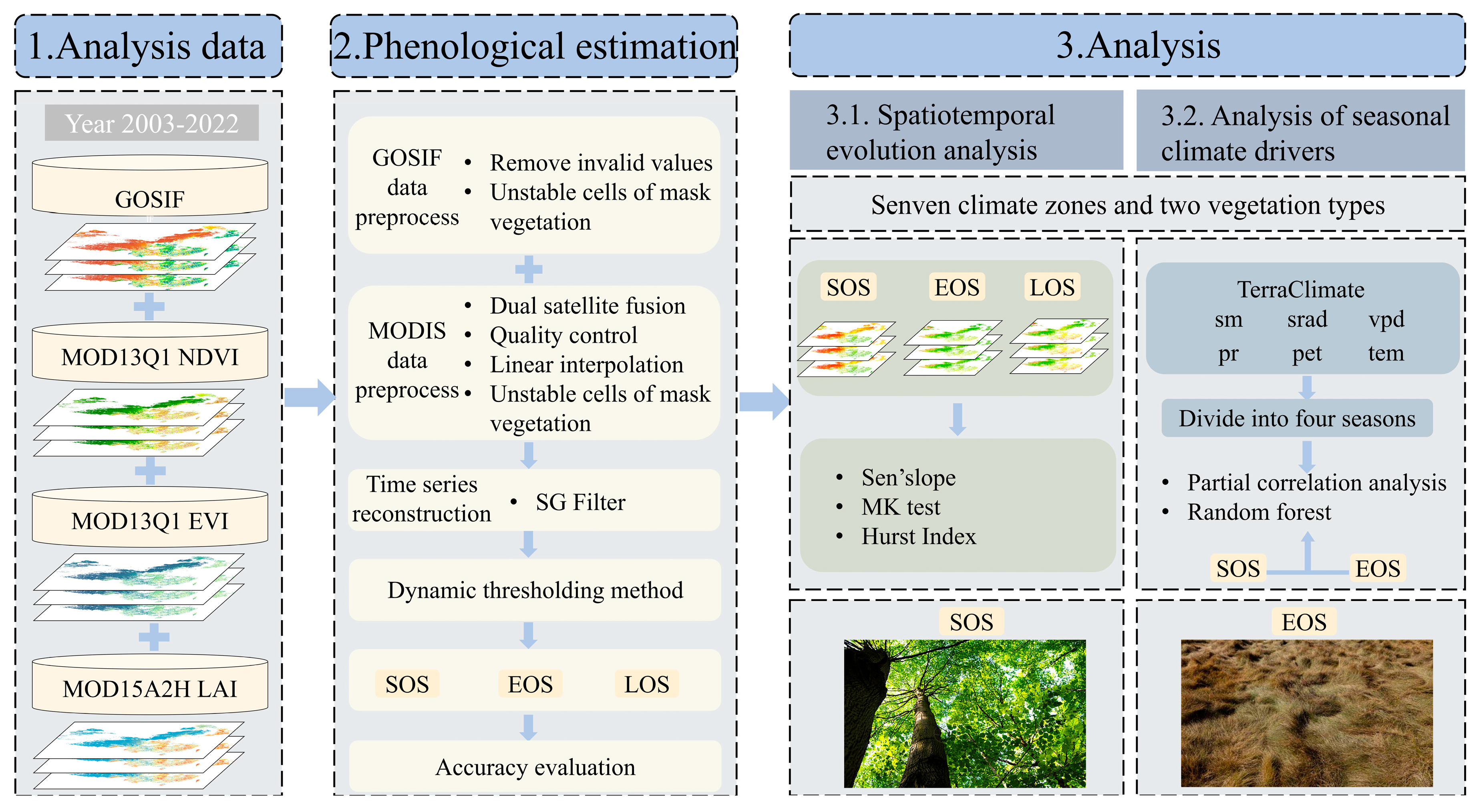
Firstly, we evaluated the accuracy of the phenological metrics derived from the four remote sensing datasets by comparing them to ground-based observational data. The Sen’s slope, Mann–Kendall (MK) test, and Hurst exponent were subsequently applied to analyze the spatiotemporal variations in phenological phases. Finally, the variance inflation factor was calculated followed by partial correlation analysis and random forest modeling to identify the major climatic drivers of SVP across the seven climate zones and two vegetation types, as well as the seasonal contributions of climate to SVP (Figure 3).

2.3.1. SVP Metrics Estimation

Remote sensing images are significantly affected by clouds and atmospheric conditions during acquisition, requiring the denoising and smoothing of temporal data. Among the four long-term remote sensing datasets, NDVI, EVI, and LAI were linearly interpolated on the GEE cloud platform, while GOSIF data were first filtered to remove invalid values and then reconstructed using the Savitzky–Golay (SG) filter method with a sliding window size of 5 to eliminate noise.
The dynamic threshold method proposed by Jönsson et al. [42] was applied to set varying thresholds at the pixel scale to obtain the vegetation SOS and EOS for each pixel. The formula is as follows:
S O S = ( I n d e x m a x I n d e x m i n )   × 20 %
E O S = ( I n d e x m a x I n d e x m i n )   ×   50 %
L O S = E O S S O S
In the formula, I n d e x represents the values of NDVI, EVI, LAI, and SIF. The threshold for identifying SOS was set at 0.2, while the threshold for EOS was set at 0.5 [43].

2.3.2. Evaluation of the Accuracy of Phenology Estimation

This study evaluates the accuracy of SOS, EOS, and LOS derived from four remote sensing datasets by using correlation coefficients (R) and regression models, comparing them with site-based observations. For each ground phenological observation site, we extracted the SOS, EOS, and LOS values estimated from the corresponding remote sensing pixel at a 0.05° resolution. The R was used to quantify the linear relationship between phenological metrics derived from remote sensing datasets and site-based observations. The correlation coefficient ranges from −1 to 1, with values closer to 1 indicating a stronger correlation.

2.3.3. Analyzing Trends and Persistence in Changes to Phenological Metrics

Sen’s slope and the Mann–Kendall (MK) test were employed to analyze trends, with the formula for calculating the Sen’s slope [44] estimator given as follows:
β = M e d i a n x j x i j i , j > i
In the formula, β represents the trend of phenological metrics changes; M e d i a n is the median function; x i , x j are the SVP values in i year and j year, respectively. When β < 0 , the phenological metric shows an advancing trend, whereas when β > 0 , it indicates a delaying trend.
Furthermore, the Mann–Kendall trend test [45,46] was applied, primarily to identify abrupt change points in the phenological series, enabling the assessment of significance and the analysis of phenological change trends. Persistence analysis was conducted using the Hurst exponent [47]. When the Hurst index equals 0.5, it indicates that the phenological time series exhibits random fluctuations and lacks long-term correlation. In contrast, when the Hurst index is greater than 0.5, the time series exhibits persistence, with future trends mirroring past trends. Conversely, when the Hurst index is less than 0.5, future trends are expected to oppose past trends.

2.3.4. Analysis of the Response of SVP to Seasonal Climate Variability

To mitigate multicollinearity, the Variance Inflation Factor (VIF) was first calculated, and variables with VIF values below 10 were retained for subsequent analysis [48]. Subsequently, higher-order partial correlation analysis was performed to investigate the relationships between SVP and seasonal climate variability, while controlling for confounding variables, to determine both the direction and significance of each climatic factor’s influence on phenology. Assume there are k k > 2 variables x 1 , x 2 x k . The partial correlation coefficient for any two variables x i and x j at the n n k 2 order sample is calculated as follows:
r i j · 1 1 1 2 1 n = r i j · 1 1 1 2 1 n 1 r i 1 n · 1 1 1 2 1 n 1 r j 1 n · 1 1 1 2 1 n 1 1 r i 1 n · 1 1 1 2 1 n 1 2 1 r j 1 n · 1 1 1 2 1 n 1 2
In the formula, r i j · 1 1 1 2 1 n represents the partial correlation coefficient between a specific phenological metric (e.g., SOS, EOS, or LOS) i and climate factor j , with control variables being the climate variables of other seasons.
Finally, a random forest regression model was employed to assess the relative importance of each climatic variable in influencing phenological metrics. The cumulative contributions of seasonal climatic factors to SVP were statistically summarized to identify the dominant seasonal drivers of SVP across the study area and within each climatic zone.

3. Results

3.1. Accuracy Assessment of SVP Estimation from Four Remote Sensing Datasets

Figure 4 illustrates the correspondence between SVP metrics derived from four remote sensing datasets and ground-based observational data. The EOS values derived from these datasets exhibit consistently high levels of accuracy across all comparisons. The SIF dataset demonstrated superior performance in estimating SOS, EOS, and LOS, with all correlation coefficients (R) exceeding 0.69 and an average of 0.75, closely aligning with phenological trends observed at ground stations. This is likely due to SIF’s ability to directly reflect vegetation photosynthetic activity and its relative insensitivity to cloud and aerosol interference, allowing for more accurate detection of actual phenological transitions, particularly the onset of vegetation activity (the R between SOS and observed values reaches as high as 0.76). In contrast, the SOS estimates derived from vegetation indices and LAI exhibit lower accuracy, with R values generally below 0.6; notably, SOS derived from NDVI shows particularly weak correlation with ground observations, yielding an R value of only 0.29. This may be attributed to the fact that NDVI primarily reflects canopy spectral properties, making it highly susceptible to interference from clouds, snow, and soil background—especially in areas with sparse vegetation or frequent cloud cover—resulting in greater uncertainties in phenological retrieval [49]. Moreover, NDVI is prone to saturation in regions with dense vegetation, hindering its ability to reliably detect subtle phenological dynamics. Although EVI partially mitigates the saturation issue, it remains susceptible to background noise, leading to lower accuracy in phenological detection compared to SIF.

3.2. Spatial Distribution of SVP in China

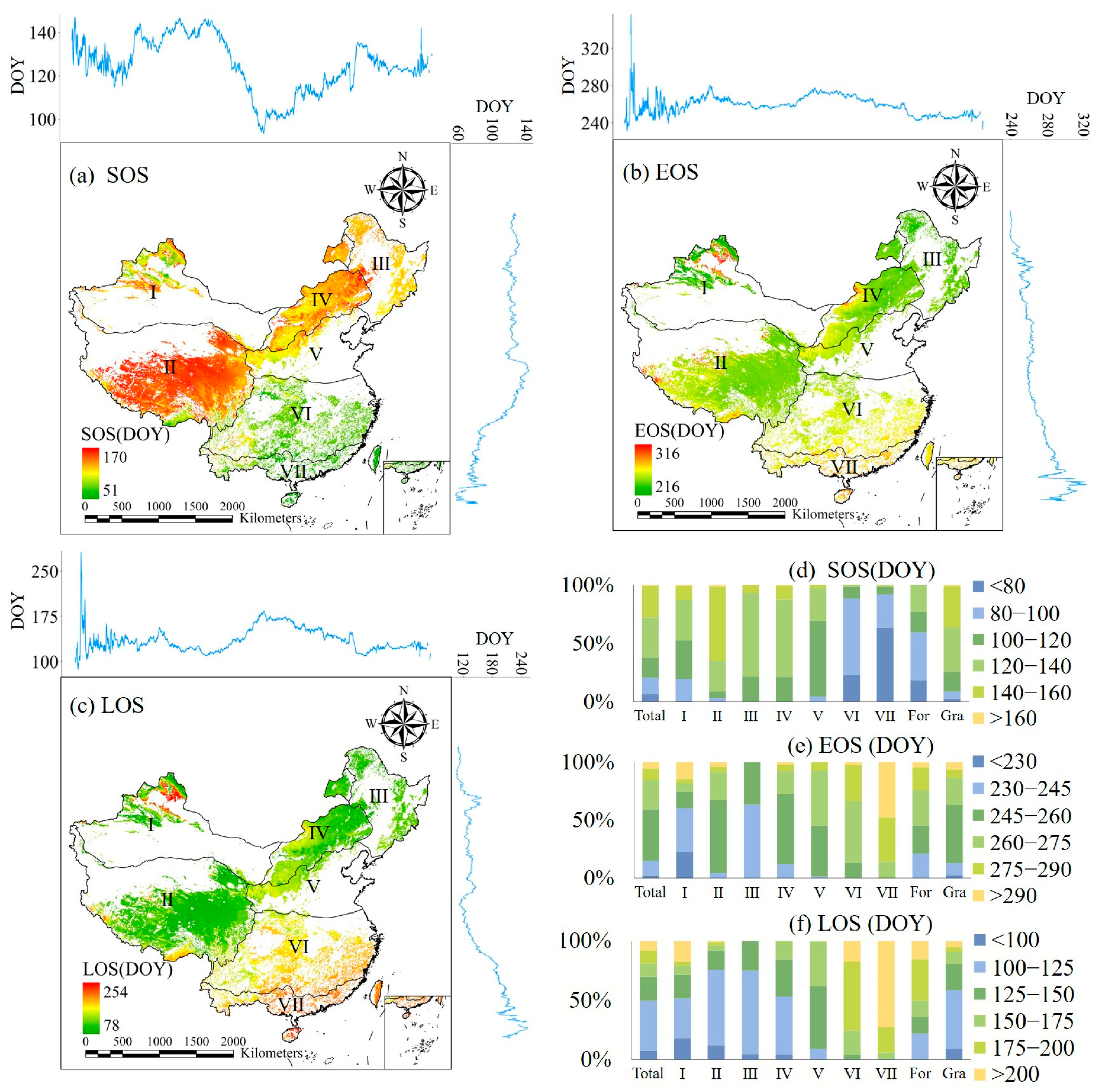
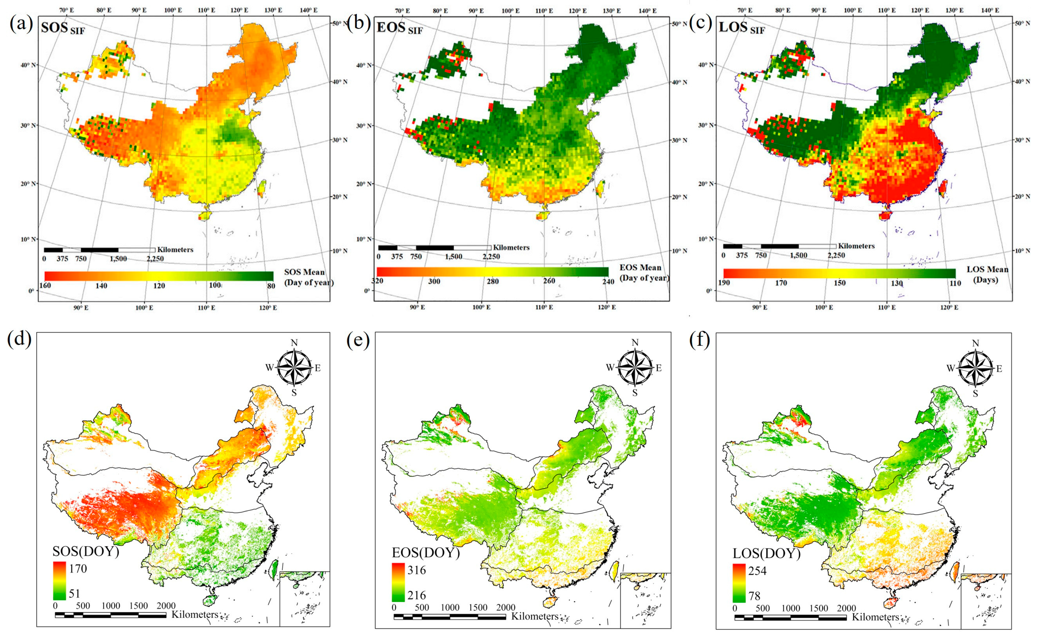
Figure 5 illustrates the spatial distribution of three SVP metrics across China, along with the corresponding value ranges of each metric. The spatial distribution of SVP in the study area can be broadly categorized into three regions: the Tibetan Plateau (Region II), the area north of the Qinling–Huaihe Line (Regions I, III, IV, and V), and the area to the south of it (Regions VI and VII). In regions south of the Qinling–Huaihe Line, vegetation exhibits an earlier SOS and a later EOS, resulting in an extended LOS; for instance, in Region VII, 72% of LOS values exceed 200 days. In the Tibetan Plateau region, vegetation experiences a delayed SOS and an earlier EOS, resulting in the shortest LOS. This phenomenon is primarily attributed to the Tibetan Plateau’s high elevation and cold climate—often referred to as the “Third Pole”—which limit the length of the vegetation growing season, with 64% of LOS values ranging from 100 to 125 days. The region north of the Qinling–Huaihe Line exhibits intermediate phenological characteristics compared to the southern and Tibetan Plateau regions.
Both longitudinally and latitudinally, the SOS shows a distinct decline at the boundary between the first stage (Tibetan Plateau) and the second stage (Sichuan Basin, Loess Plateau, and Yunnan-Guizhou Plateau) steps, before transitioning into a gradual delay. However, there is minimal variation in EOS along the longitudinal direction; conversely, in the latitudinal direction, the SOS shows a clear trend of earlier onset in the southern regions of China. In contrast, the EOS and LOS exhibit opposite trends. This suggests that the latitudinal variation in SVP is more pronounced than the longitudinal variation. These significant regional differences suggest that climate factors such as temperature, precipitation, and solar radiation, influenced by altitude and latitude, have an important impact on SVP.
Moreover, the SOS in forests generally occurs earlier than in grasslands, and the LOS of forests tends to be longer. This may be attributed to the predominance of forests in southern China and their greater capacity to acquire water and nutrients, which enables earlier growth initiation. In contrast, grasslands are primarily distributed in northern China, where growth is more constrained by environmental factors such as temperature and water availability, resulting in a relatively shorter phenological period.

3.3. Spatiotemporal Evolution of SVP in China

Figure 6 illustrates the changes in SVP in China over the past two decades, along with projections for future trends. Table 2 and Table 3 provide a summary of various change types and future trends observed over the past two decades. The results reveal that vegetation SOS advanced, accounting for up to 74.96%, with 18.79% of the area showing significant advance (p < 0.05), primarily in southern China, resulting in an extension of the LOS in this area. However, the proportion of advanced and delayed vegetation EOS are comparable, with 36.90% of the regions exhibiting a delayed trend and 51.76% exhibiting an advanced trend. The delayed regions were primarily located in the western part of the Tibetan Plateau (Region II) and the eastern part of Inner Mongolia (Region IV), contributing to the extension of LOS in these areas. The advance areas are primarily located in the eastern Qinghai–Tibet Plateau (Zone II), western Inner Mongolia (Zone IV), and the southeastern coastal regions, leading to the shortening of LOS in these areas.
Regarding future trends, the SVP in most parts of China remains unstable (greater than 70%), with the vegetation LOS is expected to shift from prolongation to shortening in the majority of the study area, accounting for 45.08%. Specifically, the proportion of SOS expected to shift from advancement to delay in the future is 57.97%. Finally, it is important noting that there are significant differences in the SVP trends between the eastern and western parts of the Tibetan Plateau (Region II) and the central and eastern parts of Inner Mongolia (Region IV), which may be attributed to the precipitation imbalance in these regions.
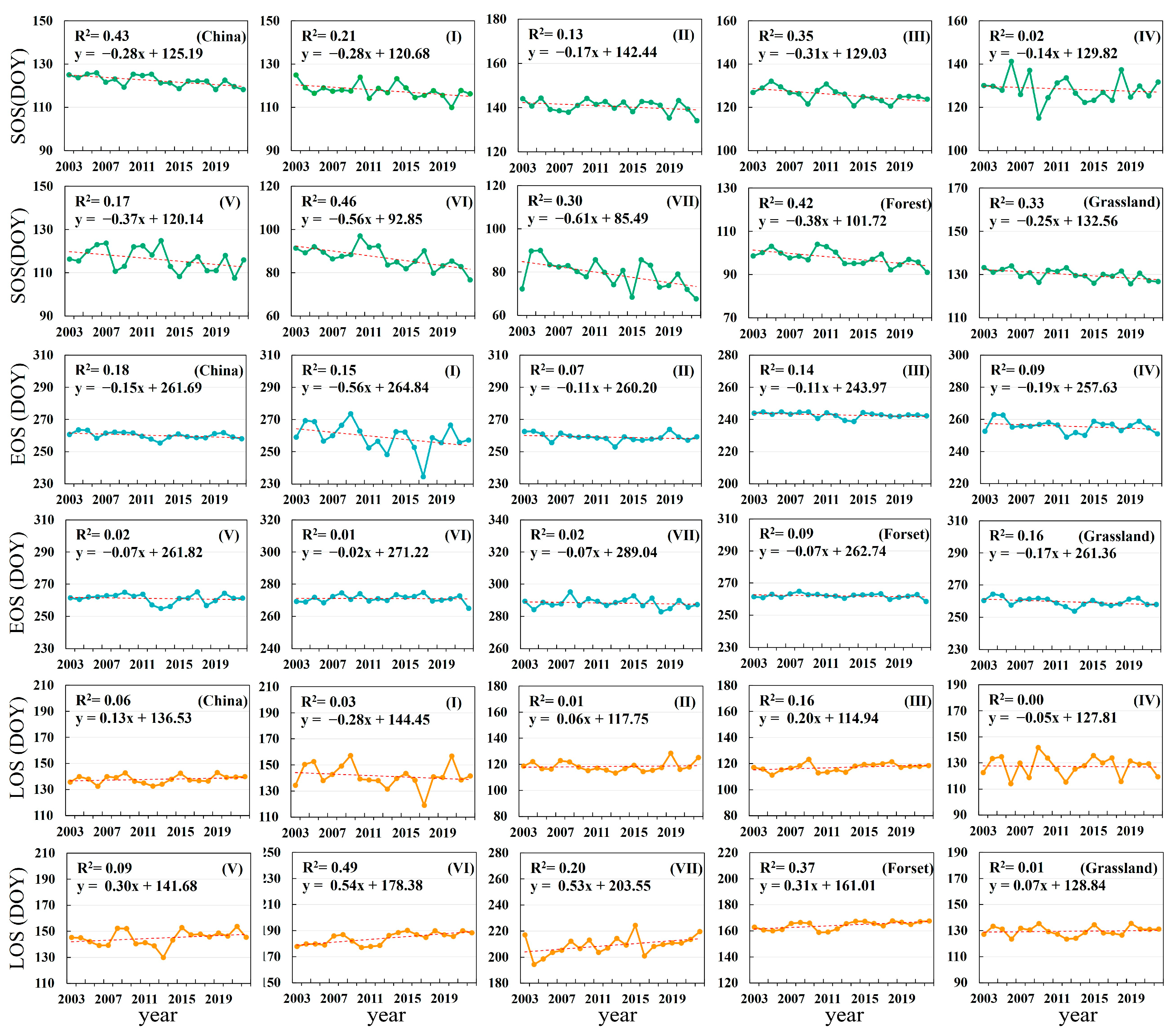
Figure 7 illustrates the interannual variation in the mean SVP metrics for the study area and seven climate zones. Significant differences in the variation in SVP metrics are observed across different climate zones and stable vegetation types. SOS exhibits an advancing trend across the entire study area and all climate zones. Further analysis reveals that SOS advances more rapidly in climate zones that are located further south and the more humid and warmer, with the fastest rate observed in Region VII, reaching a slope of −0.61 days per year. Although EOS generally shows stable trend (with small R2 values) across the study area and most climate zones, it is clear that the advancement rate of EOS is greater in drier regions—for example, in the arid Region I, the advancement rate of EOS reaches 0.56 days per year. The regional disparity between SOS and EOS directly results in an overall extension of the LOS across the study area, particularly in southern China—reaching as high as 0.54 days per year in Region VI. Moreover, regarding the trends of phenological metrics for stable vegetation types, the SOS in forests advances at a rate 0.13 days per year faster than in grasslands, while the EOS in forests advances 0.10 days per year slower than in grasslands. As a result, the LOS in forests increases 0.24 days per year compared to in grasslands.

3.4. Effects of Seasonal Climate Factor Changes on SVP

Figure 8 illustrates the relationships between stable vegetation SOS and the driving climatic factors, analyzed across different climate zones and vegetation types. Throughout the study area, stable vegetation SOS is primarily influenced by spring climate (contribution rate up to 70%), exhibiting a significant negative correlation (r = −0.38 and −0.53, respectively; p < 0.05) with winter sm and spring tem, with the latter being the dominant contributing factor (contribution rate up to 55%). This may be attributed to higher winter sm, which ensures adequate water supply for spring vegetation germination, while elevated spring tem directly promote an earlier start to the growing season, thus leading to an earlier SOS. Across various regions, Region IV, a temperate semi-arid zone, is primarily influenced by winter tem, resulting in a greater delay in stable vegetation SOS (Figure 6), and ultimately leading to the lowest rate of SOS advancement in the region (Figure 7). In all other climate zones, stable vegetation SOS is predominantly influenced by spring tem or vpd.
In regions with significant relationships (p < 0.05), SOS and spring tem exhibit a negative correlation, indicating that rising spring temperatures lead to earlier SOS. However, the partial correlation coefficients between SOS and vpd display both positive and negative values. For example, in relatively warm and humid regions such as Zones V and VI, the coefficients are positive (r = 0.67 and 0.56, respectively). This may be due to lower vpd, which indicates increased atmospheric humidity, generally enhancing plant water-use efficiency, promotes growth, and resulting in an earlier SOS. In relatively arid and cold regions, such as Zone I, a negative correlation is observed (r = −0.41). In these regions, a higher vpd indicates limited water availability, which may inhibit plant growth and delay the onset of the growing season due to prolonged environmental constraints. For stable vegetation types, the SOS for both forests and grasslands showed a significant negative correlation (p < 0.05) with them. However, while forest SOS was negatively correlated only with spring tem (r = −0.65), grassland SOS was negatively correlated with both spring and winter tem (r = −0.49 and −0.45, respectively), suggesting that grasslands are more sensitive to accumulated tem.
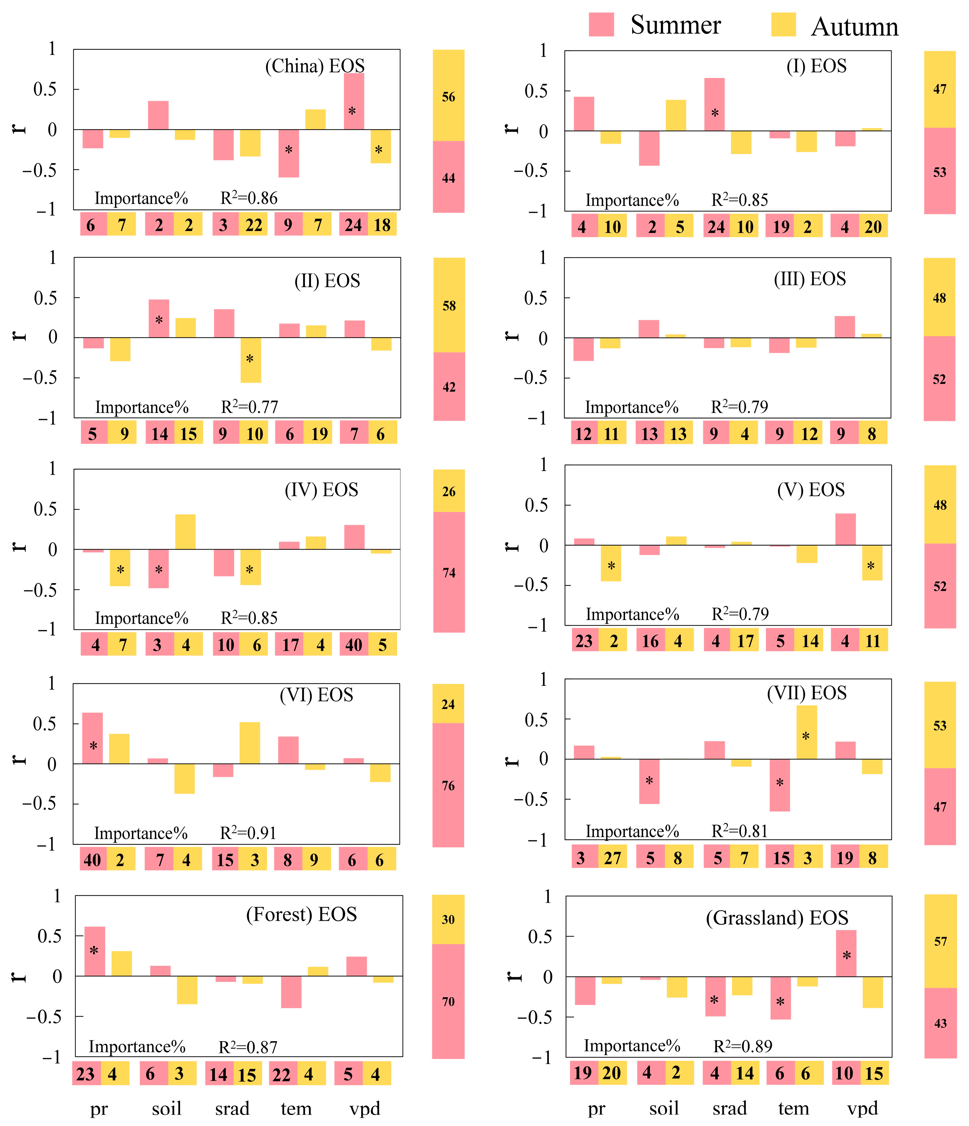
Figure 9 illustrates the relationships between stable vegetation EOS and the driving climatic factors, analyzed across different climate zones and vegetation types. The vegetation EOS across the entire study area is primarily influenced by autumn climatic conditions, exhibiting a strong positive partial correlation with summer vpd (r = 0.77, p < 0.05) and an inverse relationship with autumn vpd (r = −0.39, p < 0.05). Moreover, the contribution of summer vpd exceeds that of autumn vpd, suggesting that an increase in summer vpd promotes an extension of the SVP metric, while an increase in autumn vpd has the opposite effect. This may be due to vpd influencing the end of the growing season by regulating water availability and plant transpiration rates.
At the regional scale, the regulation of stable vegetation EOS is relatively complex, with distinct dominant climatic factors and seasons across different climate zones. Stable vegetation EOS on the Tibetan Plateau is primarily regulated by autumn climatic conditions (contribution rate up to 58%), while in most other regions, it is predominantly influenced by summer climate. In the arid Region I, stable EOS is primarily influenced by summer srad, exhibiting a positive correlation (r = 0.70, p < 0.05). In the relatively moist Region VI, it is predominantly influenced by the summer pr (contribution rate up to 40%), also exhibiting a positive correlation (r = 0.58, p < 0.05). It is noteworthy that in most climate zones, the effects of summer and autumn vpd on stable vegetation EOS are opposite, consistent with the seasonal differences observed across the study area, though variations exist among regions. In general, in arid and cold regions, the inherently high vpd causes plants to terminate growth earlier, while in warm and humid regions, the relatively low vpd promotes longer growing metrics, thereby delaying EOS. For different vegetation types, the effects of summer and autumn vpd on EOS exhibit opposite directions in grasslands and forests. However, grassland EOS is significantly influenced by three summer climatic factors—tem, srad, and vpd (r = −0.53, r = −0.49 and r = 0.58, respectively; p < 0.05)—whereas forest EOS is significantly affected only by summer pr (r = 0.61, p < 0.05). In addition, more climatic factors significantly influencing SOS in grassland than in forests (Figure 8), indicating that grasslands are more sensitive to seasonal climatic variations than forests. This sensitivity may be attributed to the predominance of shallow-rooted herbaceous species in grasslands, which have limited physiological regulation capacity and are therefore more responsive to seasonal climate fluctuations. In contrast, forests are dominated by deep-rooted woody species with greater environmental adaptability and regulatory capacity. The dominant factors influencing EOS vary across stable vegetation types and climate zones, indicating that the termination of the growing season is driven by multiple seasonal climatic drivers.

4. Discussion

4.1. Performance Differences in VP Retrieval Using Multi-Source Remote Sensing Data

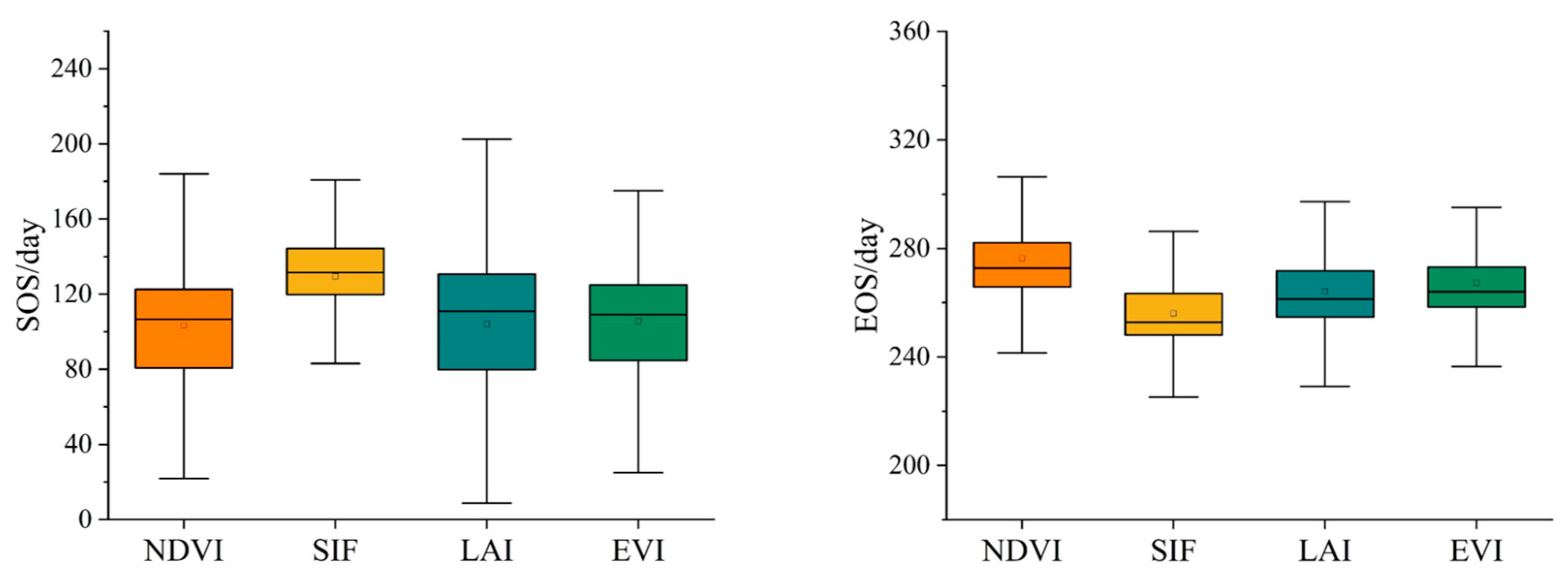
This study systematically compared the estimation of SVP using four remote sensing products—SIF, NDVI, EVI, and LAI—and found that SIF data outperformed the others in monitoring SVP (Figure 4). This is consistent with the findings of Zhang et al. [50]. Currently, most studies on VP are based on vegetation indices (VIs) [5,7]. Although VIs is closely related to vegetation cover and greenness, they do not fully capture the actual phenological status of plant photosynthetic processes [51,52,53,54]. SIF is the energy flux re-emitted by plants during photosynthesis, reflecting the efficiency of photosynthetic utilization [55]. It is more directly related to photosynthesis and can effectively monitor VP [22,56]. Generally, vegetation begins to green before photosynthesis is activated, and as it enters senescence, photosynthetic activity diminishes significantly, even before the leaves turn yellow [17]. Consequently, the SOS derived from SIF is typically later than that from VIs, while the EOS estimated by SIF tends to occur earlier than that from VIs (Figure 10). Additionally, this study revealed that among the vegetation indices (VIs), NDVI exhibited the weakest correlation with site-based observations (Figure 4), likely due to its susceptibility to soil background interference and signal saturation in areas with high vegetation cover [49]. Although EVI attempts to address this limitation and demonstrates greater accuracy than NDVI in vegetation phenology monitoring (Figure 4), the issue of saturation remains present [11]. In summary, VIs may become insensitive due to saturation, leading to biases in phenology metric estimation.

4.2. The Spatiotemporal Evolution Patterns of SVP in China

The spatial distribution of SVP in China is broadly categorized into three regions: the Tibetan Plateau (Region II), north of the Qinling–Huaihe Line (Regions I, III, IV, V), and south of the Qinling–Huaihe Line (Regions VI, VII). This is generally consistent with the three spatial distribution patterns of vegetation phenology identified in Wang Xin’s study [22] at a macro scale (Figure 11). In contrast to other large-scale SIF studies [22,23], this study employed SIF data with a higher spatial resolution (0.05°), allowing for a more precise capture of regional phenology heterogeneity. In VP derived from lower-resolution data, a single pixel may encompass multiple land cover types, making phenology estimation more susceptible to the mixed-pixel effect [57], thereby leading to blurred and anomalous phenological metrics (Figure 11).
Additionally, this study found that the proportion of pixels with earlier EOS was approximately 15% higher than those with delayed EOS (Table 2), with most earlier EOS regions concentrated in the water-heat balance zone. This finding contrasts with conclusions from other large-scale studies, which indicate a greater prevalence of delayed EOS pixels [58]. The primary reason is that this study focused on multi-year stable vegetation, effectively excluding short-term vegetation in agricultural regions where phenology may be delayed by cropping practices. For example, the study by Wang et al. [59] indicated that maize growth duration in northern China lengthened from 1981 to 2010 due to cultivar shifts. Eyshi Rezaei et al. [27] also found that the period from maturity to harvest for rapeseed and rye significantly lengthened due to management practices. On the other hand, it effectively excluded vegetation in urban areas where EOS was significantly delayed by non-climatic factors such as the urban heat island effect. For instance, Ji et al. [60], showed that in over 1500 cities across China, areas with delayed vegetation EOS substantially outnumbered those with advanced EOS. Yao et al. [61] found that the average EOS in urban areas of Beijing was delayed by 18.9 days compared to rural areas. Failure to exclude these human-impacted areas could exaggerate the trend of delayed EOS and obscure the fundamental response of natural vegetation to climate change. This finding ensures the accuracy of analyzing the phenological response of stable natural vegetation to seasonal climate variations.

4.3. Characteristics of SVP in China Regulated by Seasonal Climate Change

This study reveals that spring tem and vpd play a key regulatory role in the stable vegetation SOS across China’s major climate zones. Spring tem is a primary driving factor in most regions, exhibiting a negative correlation with SOS. Warming accelerates the accumulation of temperature, prompting vegetation to reach the thermal threshold for spring germination earlier [62], consistent with findings in temperate and cold regions where warming accelerates SOS [63]. In the water-sensitive semi-arid region (Regions IV), high spring vpd intensifies evapotranspiration, leading to water stress [64]. This explains why the advance of phenology in this region is limited, suggesting that water availability may modulate or even restrict the impact of tem on phenology in arid regions.
The climate factors driving vegetation EOS and the dominant seasonal climate display a highly complex regulatory pattern [65]. Chen et al. [66] found that changes in solar radiation are a precursor to leaf shedding, while Li et al. [67] demonstrated that vpd negatively impacts vegetation growth. However, they did not elucidate the mechanism by which climate factors drive EOS changes across different seasons. This study found that EOS is positively correlated with summer vpd and negatively correlated with autumn vpd. The spatiotemporal differentiation of these positive and negative effect suggests that vpd in different seasons regulates EOS through a dual “limiting-promoting” mechanism affecting vegetation water conditions. The conclusion that summer vpd is positively correlated with EOS aligns with the findings of Wang et al. [68]. This study further found that autumn vpd is negatively correlated with stable vegetation EOS. Under the context of global warming, vpd continues to increase [69], leading to higher water vapor loss to the atmosphere through plant transpiration and soil evaporation. This condition hinders plant growth and the continuation of photosynthesis [69], leading to an earlier EOS.
Moreover, the differences in phenological responses to seasonal climate variations among different stable vegetation types should not be overlooked. This study found that grasslands are more sensitive to seasonal climate changes, which is consistent with the findings of Jia et al. [70]. However, this study further revealed that accumulated tem had a stronger influence on the SOS in grasslands, while summer pr played a key role in regulating the EOS in forests. These results underscore the importance of accounting for the complex interactions between seasonal climate drivers and different stable vegetation types in understanding SVP.

4.4. Limitations and Future

This study solely utilized spectral data for the estimation of SVP, which may be affected by cloud cover, rainfall, and non-vegetation land types, potentially leading to inaccuracies in phenology estimation. Future research could integrate optical data with radar data to establish a more robust observation system. By combining multi-temporal and multi-sensorial data, the analysis of phenological trends across various scales and ecological contexts could be improved. This study employed a single time-series reconstruction method and phenological parameter estimation technique, while the dynamic threshold method may introduce certain errors due to differences in study regions and vegetation types. Since the lack of a unified standard for phenological estimation [63], some studies calculate the average of results from different methods as the final outcome of large-scale regional phenological research, thereby reducing uncertainties due to methodological differences [71]. With the advancement of algorithms such as deep learning, methods like LSTM [72] and Transformer [73], which can account for both data feature complexity and temporal dependencies, could be introduced to more efficiently learn phenological change patterns from remote sensing time series.

5. Conclusions

A comprehensive analysis of the long-term dynamics of SVP in China and its response to seasonal climatic variations is crucial for gaining a deeper understanding of ecological changes in the region. First, SIF data showed the closest agreement with ground-based observations in estimating SVP, with R values for the three phenological metrics all exceeding 0.69 and an average value of 0.75. The spatial distribution of SVP in China revealed three distinct spatial patterns: the Tibetan Plateau region (Zone II), the area north of the Qinling–Huaihe Line (Zones I, III, IV, and V), and the area south of the Qinling–Huaihe Line (Zones VI and VII). From arid, cold-to-warm, and humid regions, the advancement rate of SOS gradually increases. EOS shifts from being advanced to remaining relatively unchanged, while the rate of LOS extension correspondingly increases. In the future, most SVP across China is projected to become unstable. Finally, the SOS for stable vegetation in China is primarily driven by the spring climate in most climate zones, with the overall contribution of the spring climate reaching 70% at the national scale. Spring temperatures generally have a negative effect on SOS (r = −0.53, p < 0.05), while EOS is regulated by a complex interplay of multiple climatic factors. Vapor pressure deficit plays a dual role of “limitation–promotion,” showing a significant negative effect in autumn (r = −0.39, p < 0.05) and a significant positive effect in summer (r = 0.77, p < 0.05). This study fills a gap in our understanding of SVP and contributes to a deeper comprehension of interannual variability in stable vegetation under seasonal climate change.

Author Contributions

Conceptualization, X.W.; Methodology, J.L. (Jian Luo), X.W., Y.G., Y.X., Q.Y., J.L. (Jiaxin Liu), Y.L., Z.D. and Q.W.; Software, J.L. (Jian Luo), Y.G., Y.C., Y.X., Z.D. and Q.W.; Validation, J.L. (Jian Luo) and Y.G.; Formal analysis, X.W.; Investigation, Y.G., Y.C. and L.Y.; Resources, X.W., L.Y. and Y.L.; Data curation, J.L. (Jian Luo), L.Y., Y.X., Q.Y., J.L. (Jiaxin Liu) and Y.L.; Writing—original draft, J.L. (Jian Luo) and X.W.; Writing—review & editing, J.L. (Jian Luo), X.W., Y.G., Y.C., L.Y., Y.X., Q.Y., J.L. (Jiaxin Liu), Y.L., Z.D. and Q.W.; Visualization, J.L. (Jian Luo) and Y.C.; Supervision, X.W. and B.L.; Project administration, X.W. and B.L.; Funding acquisition, X.W. All authors have read and agreed to the published version of the manuscript.

Funding

This research was supported by the Natural Science Foundation of Sichuan Province, China (grant numbers 2025ZNSFSC0329, 25NSFJQ0136), Natural Resources Research Project of Sichuan Province (grant numbers KJ-2025-61), Deployment project of the Overseas Science and Education Cooperation Center, Bureau of International Cooperation, Chinese Academy of Sciences (grant number 162GJHZ2023065MI), and the National Natural Science Foundation of China (grant number 42361144855).

Data Availability Statement

The original contributions presented in the study are included in the article, further inquiries can be directed to the corresponding author.

Conflicts of Interest

The authors declare no conflict of interest.

References

  1. Lieth, H. (Ed.) Phenology and Seasonality Modeling; Springer: Berlin/Heidelberg, Germany, 1974; p. 4. [Google Scholar]
  2. Peters-Lidard, C.D.; Zion, M.S.; Wood, E.F. A soil-vegetation-atmosphere transfer scheme for modeling spatially variable water and energy balance processes. J. Geophys. Res. Atmos. 1997, 102, 4303–4324. [Google Scholar] [CrossRef]
  3. Root, T.L.; Price, J.T.; Hall, K.R.; Schneider, S.H.; Rosenzweig, C.; Pounds, J.A. Fingerprints of global warming on wild animals and plants. Nature 2003, 421, 57–60. [Google Scholar] [CrossRef]
  4. Chen, X.; Hu, B.; Yu, R. Spatial and temporal variation of phenological growing season and climate change impacts in temperate eastern China. Glob. Change Biol. 2005, 11, 1118–1130. [Google Scholar] [CrossRef]
  5. Chang, Q.; Xiao, X.; Jiao, W.; Wu, X.; Doughty, R.; Wang, J.; Du, L.; Zou, A.; Qin, Y. Assessing consistency of spring phenology of snow-covered forests as estimated by vegetation indices, gross primary production, and solar-induced chlorophyll fluorescence. Agric. For. Meteorol. 2019, 275, 305–316. [Google Scholar] [CrossRef]
  6. Yang, X.; Mustard, J.F.; Tang, J.; Xu, H. Regional-scale phenology modeling based on meteorological records and remote sensing observations. J. Geophys. Res. Biogeosci. 2012, 117, G03029. [Google Scholar] [CrossRef]
  7. Hmimina, G.; Dufrêne, E.; Pontailler, J.-Y.; Delpierre, N.; Aubinet, M.; Caquet, B.; De Grandcourt, A.; Burban, B.; Flechard, C.R.; Granier, A.; et al. Evaluation of the potential of MODIS satellite data to predict vegetation phenology in different biomes: An investigation using ground-based NDVI measurements. Remote Sens. Environ. 2013, 132, 145–158. [Google Scholar] [CrossRef]
  8. Melaas, E.K.; Friedl, M.A.; Zhu, Z. Detecting interannual variation in deciduous broadleaf forest phenology using Landsat TM/ETM+ data. Remote Sens. Environ. 2013, 132, 176–185. [Google Scholar] [CrossRef]
  9. Zhang, X.; Friedl, M.A.; Schaaf, C.B.; Strahler, A.H.; Hodges, J.C.F.; Gao, F.; Reed, B.C.; Huete, A. Monitoring vegetation phenology using MODIS. Remote Sens. Environ. 2003, 84, 471–475. [Google Scholar] [CrossRef]
  10. Tucker, C.J. Red and photographic infrared linear combinations for monitoring vegetation. Remote Sens. Environ. 1979, 8, 127–150. [Google Scholar] [CrossRef]
  11. Huete, A.; Didan, K.; Miura, T.; Rodriguez, E.P.; Gao, X.; Ferreira, L.G. Overview of the radiometric and biophysical performance of the MODIS vegetation indices. Remote Sens. Environ. 2002, 83, 195–213. [Google Scholar] [CrossRef]
  12. Xiang, Y.; Xiao, Z.; Liang, S.; Wang, J.; Song, J. Validation of Global LAnd Surface Satellite (GLASS) leaf area index product. J. Remote Sens. 2014, 18, 573–588. [Google Scholar] [CrossRef]
  13. Pinzon, J.E.; Tucker, C.J. A non-stationary 1981–2012 AVHRR NDVI3g time series. Remote Sens. 2014, 6, 6929–6960. [Google Scholar] [CrossRef]
  14. Zhou, Y.K.; Zhang, R.X.; Sun, W.B.; Zhang, S.H. Spatial and temporal characteristics of vegetation phenology in the Northeast China based on sun-induced chlorophyll fluorescence and its response to climate. Remote Sens. Technol. Appl. 2024, 39, 185–197. [Google Scholar]
  15. Wang, M.Y.; Luo, Y.; Zhang, Z.Y.; Xie, Q.Y.; Wu, X.D.; Ma, X.L. Recent advances in remote sensing of vegetation phenology: Retrieval algorithm and validation strategy. Natl. Remote Sens. Bull. 2022, 26, 431–455. [Google Scholar] [CrossRef]
  16. Bertani, G.; Wagner, F.H.; Anderson, L.O.; Aragão, L.E.O.C. Chlorophyll fluorescence data reveals climate-related photosynthesis seasonality in Amazonian forests. Remote Sens. 2017, 9, 1275. [Google Scholar] [CrossRef]
  17. Joiner, J.; Yoshida, Y.; Vasilkov, A.P.; Schaefer, K.; Jung, M.; Guanter, L.; Zhang, Y.; Garrity, S.; Middleton, E.; Huemmrich, K.; et al. The seasonal cycle of satellite chlorophyll fluorescence observations and its relationship to vegetation phenology and ecosystem atmosphere carbon exchange. Remote Sens. Environ. 2014, 152, 375–391. [Google Scholar] [CrossRef]
  18. Piao, S.; Liu, Q.; Chen, A.; Janssens, I.A.; Fu, Y.; Dai, J.; Liu, L.; Lian, X.; Shen, M.; Zhu, X. Plant phenology and global climate change: Current progresses and challenges. Glob. Change Biol. 2019, 25, 1922–1940. [Google Scholar] [CrossRef] [PubMed]
  19. Porcar-Castell, A.; Tyystjärvi, E.; Atherton, J.; Van der Tol, C.; Flexas, J.; Pfündel, E.E.; Moreno, J.; Frankenberg, C.; Berry, J.A. Linking chlorophyll a fluorescence to photosynthesis for remote sensing applications: Mechanisms and challenges. J. Exp. Bot. 2014, 65, 4065–4095. [Google Scholar] [CrossRef] [PubMed]
  20. Jeong, S.-J.; Schimel, D.; Frankenberg, C.; Drewry, D.T.; Fisher, J.B.; Verma, M.; Berry, J.A.; Lee, J.-E.; Joiner, J. Application of satellite solar-induced chlorophyll fluorescence to understanding large-scale variations in vegetation phenology and function over northern high latitude forests. Remote Sens. Environ. 2017, 190, 178–187. [Google Scholar] [CrossRef]
  21. Lu, X.; Liu, Z.; Zhou, Y.; Liu, Y.; An, S.; Tang, J. Comparison of phenology estimated from reflectance-based indices and solar-induced chlorophyll fluorescence (SIF) observations in a temperate forest using GPP-based phenology as the standard. Remote Sens. 2018, 10, 932. [Google Scholar] [CrossRef]
  22. Wang, X.; Sun, Z.; Lu, S.; Zhang, Z. Comparison of phenology estimated from monthly vegetation indices and solar-induced chlorophyll fluorescence in China. Front. Earth Sci. 2022, 10, 802763. [Google Scholar] [CrossRef]
  23. Zhou, H.; Sun, H.; Shi, Z.; Peng, F.; Lin, Y. Solar-induced chlorophyll fluorescence data-based study on the spatial and temporal patterns of vegetation phenology in the Northern Hemisphere during the period of 2007—2018. Natl. Remote Sens. Bull. 2023, 27, 376–393. [Google Scholar] [CrossRef]
  24. Bao, Y.; Tian, H.; Wang, X. Effects of climate change and ozone on vegetation phenology on the Tibetan Plateau. Sci. Total Environ. 2024, 932, 172780. [Google Scholar] [CrossRef]
  25. Zhang, R.; Qi, J.; Leng, S.; Wang, Q. Long-term vegetation phenology changes and responses to preseason temperature and precipitation in Northern China. Remote Sens. 2022, 14, 1396. [Google Scholar] [CrossRef]
  26. Ji, Z.X.; Pei, T.T.; Chen, Y.; Qin, G.X.; Hou, Q.Q.; Xie, B.P.; Wu, H.W. Vegetation phenology changes and its response to seasonal climate changes on the Loess Plateau. Acta Ecol. Sin. 2021, 41, 6600–6612. [Google Scholar] [CrossRef]
  27. Rezaei, E.E.; Siebert, S.; Ewert, F. Climate and management interaction cause diverse crop phenology trends. Agric. For. Meteorol. 2017, 233, 55–70. [Google Scholar] [CrossRef]
  28. Sacks, W.J.; Kucharik, C.J. Crop management and phenology trends in the US Corn Belt: Impacts on yields, evapotranspiration and energy balance. Agric. For. Meteorol. 2011, 151, 882–894. [Google Scholar] [CrossRef]
  29. Zhou, Q.; Yang, P.; Wu, W.; Chen, Z.; Tang, H.; Shibasaki, R. Characterizing spatial patterns of phenology in cropland of China based on remotely sensed data. Agric. Sci. China 2010, 9, 101–112. [Google Scholar] [CrossRef]
  30. Liu, F.S.; Chen, Y.; Shi, W.J.; Zhang, S.; Tao, F.L.; Ge, Q.S. Influences of agricultural phenology dynamics on land surface biophysical processes and climate feedback: A review. Acta Geol. Sin. 2017, 72, 1139–1150. [Google Scholar] [CrossRef]
  31. Forrest, J.; Miller-Rushing, A.J. Toward a synthetic understanding of the role of phenology in ecology and evolution. Philos. Trans. R. Soc. B 2010, 365, 3101–3112. [Google Scholar] [CrossRef]
  32. Liu, Q.; Fu, Y.H.; Zhu, Z.; Liu, Y.; Liu, Z.; Huang, M.; Janssens, I.A.; Piao, S. Delayed autumn phenology in the Northern Hemisphere is related to change in both climate and spring phenology. Glob. Change Biol. 2016, 22, 3702–3712. [Google Scholar] [CrossRef] [PubMed]
  33. Liu, Q.; Fu, Y.H.; Zeng, Z.; Huang, M.; Li, X.; Piao, S. Temperature, precipitation, and insolation effects on autumn vegetation phenology in temperate China. Glob. Change Biol. 2016, 22, 644–653. [Google Scholar] [CrossRef] [PubMed]
  34. Yu, H.; Luedeling, E.; Xu, J. Winter and spring warming result in delayed spring phenology on the Tibetan Plateau. Proc. Natl. Acad. Sci. USA 2010, 107, 22151–22156. [Google Scholar] [CrossRef] [PubMed]
  35. Shen, X.; Liu, B.; Xue, Z.; Jiang, M.; Lu, X.; Zhang, Q. Spatiotemporal variation in vegetation spring phenology and its response to climate change in freshwater marshes of Northeast China. Sci. Total Environ. 2019, 666, 1169–1177. [Google Scholar] [CrossRef]
  36. Jiang, K.; Bao, G. Changes in vegetation green-up period on the Mongolian Plateau from 2001 to 2017 and its response to climate change. Acta Ecol. Sin. 2019, 38, 2490. [Google Scholar]
  37. Menzel, A.; Sparks, T.H.; Estrella, N.; Koch, E.; Aasa, A.; Ahas, R.; Alm-Kübler, K.; Bissolli, P.; Braslavská, O.; Briede, A.; et al. European phenological response to climate change matches the warming pattern. Glob. Change Biol. 2006, 12, 1969–1976. [Google Scholar] [CrossRef]
  38. Hu, Y.; Fu, B.; Michaelides, K.; De Kauwe, M.G.; Wang, J.; Shen, M.; Zhang, W.; Wang, Y.; Xiao, X.; Qin, Y.; et al. Contrasting Trends in Onset of Spring Green-Up Between Grasslands and Forests in China. Earth’s Future 2025, 13, e2024EF005379. [Google Scholar] [CrossRef]
  39. Ministry of Natural Resources of the People’s Republic of China. Standard Map Service. Available online: http://bzdt.ch.mnr.gov.cn/ (accessed on 1 October 2024).
  40. Zhao, S.Q. A new scheme for comprehensive natural geographical zoning in China. Acta Geogr. Sin. 1983, 38, 1–10. [Google Scholar]
  41. Li, X.; Xiao, J. A global, 0.05-degree product of solar-induced chlorophyll fluorescence derived from OCO-2, MODIS, and reanalysis data. Remote Sens. 2019, 11, 517. [Google Scholar] [CrossRef]
  42. Jönsson, P.; Eklundh, L. Seasonality extraction by function fitting to time-series of satellite sensor data. IEEE Trans. Geosci. Remote Sens. 2002, 40, 1824–1832. [Google Scholar] [CrossRef]
  43. Ni, L. Changes in Grassland Phenology in China over the Past 30 Years and Its Response to Climatic Factors. Master’s Thesis, Gansu Agricultural University, Lanzhou, China, 2019. [Google Scholar]
  44. Sen, P.K. Estimates of the regression coefficient based on Kendall’s tau. J. Am. Stat. Assoc. 1968, 63, 1379–1389. [Google Scholar] [CrossRef]
  45. Kendall, M.G. Rank Correlation Methods; Griffin: London, UK, 1948. [Google Scholar]
  46. Mann, H.B. Nonparametric tests against trend. Econometrica 1945, 13, 245–259. [Google Scholar] [CrossRef]
  47. Hurst, H.E. Long-term storage capacity of reservoirs. Trans. Am. Soc. Civ. Eng. 1951, 116, 770–799. [Google Scholar] [CrossRef]
  48. Venter, Z.S.; Chakraborty, T.; Lee, X. Crowdsourced air temperatures contrast satellite measures of the urban heat island and its mechanisms. Sci. Adv. 2021, 7, eabb9569. [Google Scholar] [CrossRef]
  49. Camps-Valls, G.; Campos-Taberner, M.; Moreno-Martínez, Á.; Walther, S.; Duveiller, G.; Cescatti, A.; Mahecha, M.D.; Muñoz-Marí, J.; García-Haro, F.J.; Guanter, L.; et al. A unified vegetation index for quantifying the terrestrial biosphere. Sci. Adv. 2021, 7, eabc7447. [Google Scholar] [CrossRef] [PubMed]
  50. Zhang, J.; Gonsamo, A.; Tong, X.; Xiao, J.; Rogers, C.A.; Qin, S.; Liu, P.; Yu, P.; Ma, P. Solar-induced chlorophyll fluorescence captures photosynthetic phenology better than traditional vegetation indices. ISPRS J. Photogramm. Remote Sens. 2023, 203, 183–192. [Google Scholar] [CrossRef]
  51. Fang, J.; Li, X.; Xiao, J.; Yan, X.; Li, B.; Liu, F. Vegetation photosynthetic phenology metrics in northern terrestrial ecosystems: A dataset derived from a gross primary productivity product based on solar-induced chlorophyll fluorescence. Earth Syst. Sci. Data 2022, 14, 5433–5450. [Google Scholar] [CrossRef]
  52. Karkauskaite, P.; Tagesson, T.; Fensholt, R. Evaluation of the plant phenology index (PPI), NDVI and EVI for start-of-season trend analysis of the Northern Hemisphere boreal zone. Remote Sens. 2017, 9, 485. [Google Scholar] [CrossRef]
  53. Meng, F.; Huang, L.; Chen, A.; Zhang, Y.; Piao, S. Spring and autumn phenology across the Tibetan Plateau inferred from normalized difference vegetation index and solar-induced chlorophyll fluorescence. Big Earth Data 2021, 5, 182–202. [Google Scholar] [CrossRef]
  54. Wu, C.; Peng, D.; Soudani, K.; Siebicke, L.; Gough, C.M.; Arain, M.A.; Bohrer, G.; Lafleur, P.M.; Peichl, M.; Gonsamo, A.; et al. Land surface phenology derived from normalized difference vegetation index (NDVI) at global FLUXNET sites. Agric. For. Meteorol. 2017, 233, 171–182. [Google Scholar] [CrossRef]
  55. Zhang, J.; Xiao, J.; Tong, X.; Zhang, J.; Meng, P.; Li, J.; Liu, P.; Yu, P. NIRv and SIF better estimate phenology than NDVI and EVI: Effects of spring and autumn phenology on ecosystem production of planted forests. Agric. For. Meteorol. 2022, 315, 108819. [Google Scholar] [CrossRef]
  56. Xu, Y.; Li, X.; Du, H.; Mao, F.; Zhou, G.; Huang, Z.; Fan, W.; Chen, Q.; Ni, C.; Guo, K. Improving extraction phenology accuracy using SIF coupled with the vegetation index and mapping the spatiotemporal pattern of bamboo forest phenology. Remote Sens. Environ. 2023, 297, 113785. [Google Scholar] [CrossRef]
  57. Huang, P.; Pu, J.W.; Zhao, Q.Q.; Li, Z.J.; Song, H.K.; Zhao, X.Q. Research progress and development trends in vegetation remote sensing information extraction. Remote Sens. Nat. Resour. 2022, 34, 10–19. [Google Scholar] [CrossRef]
  58. Xue, Y.Y. Response of Vegetation Photosynthetic Phenology to Temperature-Precipitation-Drought in China. Master’s Thesis, Guizhou Normal University, Guiyang, China, 2024. [Google Scholar]
  59. Wang, Z.; Chen, J.; Li, Y.; Li, C.; Zhang, L.; Chen, F. Effects of climate change and cultivar on summer maize phenology. Int. J. Plant Prod. 2016, 10, 509–526. [Google Scholar] [CrossRef]
  60. Ji, Y.; Zhan, W.; Du, H.; Wang, S.; Li, L.; Xiao, J.; Liu, Z.; Huang, F.; Jin, J. Urban-rural gradient in vegetation phenology changes of over 1500 cities across China jointly regulated by urbanization and climate change. ISPRS J. Photogramm. Remote Sens. 2023, 205, 367–384. [Google Scholar] [CrossRef]
  61. Yao, J.H.; Ding, H.Y. Temporal and spatial variation characteristics analysis of vegetation phenology in Beijing based on MODIS time-series data. Remote Sens. Nat. Resour. 2024, 36, 1–10. [Google Scholar]
  62. Piao, S.; Friedlingstein, P.; Ciais, P.; Viovy, N.; Demarty, J. Growing season extension and its impact on terrestrial carbon cycle in the Northern Hemisphere over the past 2 decades. Glob. Biogeochem. Cycles 2007, 21, GB3018. [Google Scholar] [CrossRef]
  63. White, M.A.; De Beurs, K.M.; Didan, K.; Inouye, D.W.; Richardson, A.D.; Jensen, O.P.; O’Keefe, J.; Zhang, G.; Nemani, R.R.; van Leeuwen, W.J.D.; et al. Intercomparison, interpretation, and assessment of spring phenology in North America estimated from remote sensing for 1982–2006. Glob. Change Biol. 2009, 15, 2335–2359. [Google Scholar] [CrossRef]
  64. Zhao, Z.; Wang, X.; Li, R.; Luo, W.; Wu, C. Impacts of climate extremes on autumn phenology in contrasting temperate and alpine grasslands in China. Agric. For. Meteorol. 2023, 336, 109495. [Google Scholar] [CrossRef]
  65. Zhang, X.; Wang, X.; Zohner, C.M.; Peñuelas, J.; Li, Y.; Wu, X.; Zhang, Y.; Liu, H.; Shen, P.; Jia, X.; et al. Declining precipitation frequency may drive earlier leaf senescence by intensifying drought stress and enhancing drought acclimation. Nat. Commun. 2025, 16, 910. [Google Scholar] [CrossRef] [PubMed]
  66. Chen, X.; Ciais, P.; Maignan, F.; Zhang, Y.; Bastos, A.; Liu, L.; Bacour, C.; Fan, L.; Gentine, P.; Goll, D.; et al. Vapor Pressure Deficit and Sunlight Explain Seasonality of Leaf Phenology and Photosynthesis Across Amazonian Evergreen Broadleaved Forest. Glob. Biogeochem. Cycles 2021, 35, e2020GB006893. [Google Scholar] [CrossRef]
  67. Li, C.; Zhang, L.; Wang, H.; Peng, L.; Yin, P.; Miao, P. Influence of vapor pressure deficit on vegetation growth in China. J. Arid Land 2024, 16, 779–797. [Google Scholar] [CrossRef]
  68. Wang, Q.F.; Lu, J.K.; Zhang, R.R. Characteristics of vegetation phenology response to drought in mid-high latitude regions of China. J. S. China Norm. Univ. (Nat. Sci. Ed.) 2024, 56, 70–79. [Google Scholar] [CrossRef]
  69. Yuan, W.; Zheng, Y.; Piao, S.; Ciais, P.; Lombardozzi, D.; Wang, Y.; Ryu, Y.; Chen, G.; Dong, W.; Hu, Z.; et al. Increased atmospheric vapor pressure deficit reduces global vegetation growth. Sci. Adv. 2019, 5, eaax1396. [Google Scholar] [CrossRef] [PubMed]
  70. Jia, Q.; Gao, X.; Jiang, Z.; Li, H.; Guo, J.; Lu, X.; Li, F.Y. Sensitivity of temperate vegetation to precipitation is higher in steppes than in deserts and forests. Ecol. Indic. 2024, 166, 112317. [Google Scholar] [CrossRef]
  71. Cong, N.; Zhang, Y.J.; Zhu, J.T. Temperature sensitivity of vegetation phenology in spring in mid-to high-latitude regions of Northern Hemisphere during the recent three decades. Chin. J. Plant Ecol. 2022, 46, 125–135. [Google Scholar] [CrossRef]
  72. Graves, A. Long Short-Term Memory. In Supervised Sequence Labelling with Recurrent Neural Networks; Springer: Berlin/Heidelberg, Germany, 2012; pp. 37–45. [Google Scholar] [CrossRef]
  73. Vaswani, A.; Shazeer, N.; Parmar, N.; Uszkoreit, J.; Jones, L.; Gomez, A.N.; Kaiser, L.; Polosukhin, I. Attention is all you need. Adv. Neural Inf. Process. Syst. 2017, 30, 5998–6008. [Google Scholar]
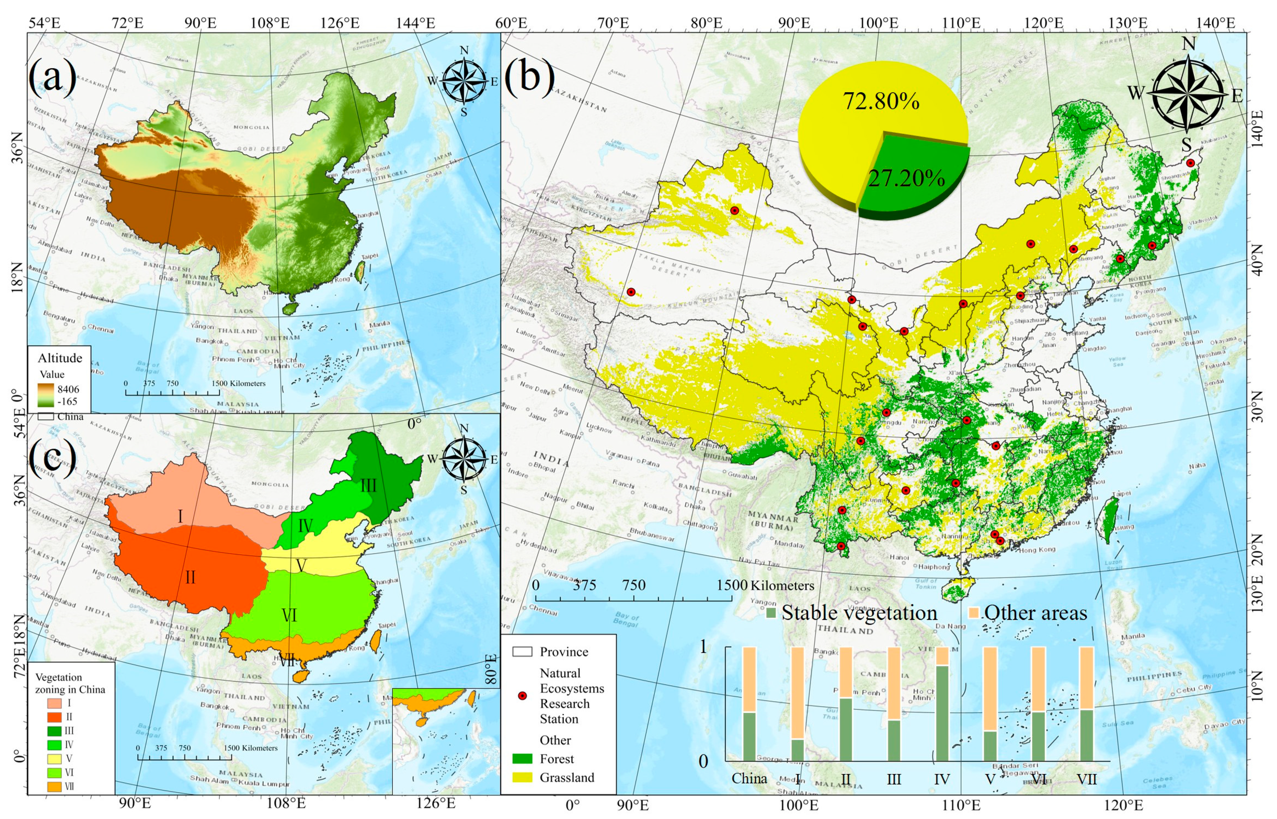
Figure 1. The elevation map of China (a). The distribution of stable vegetation across China and the locations of ground-based phenological observation sites (b). The pie chart in panel b shows the proportion of stable vegetation types in China, while the bar chart displays the ratio of stable vegetation areas to other land cover types within each climatic zone. The division of China into seven climatic zones (c). Zones I–VII correspond to the mid-temperate arid region, plateau temperate semi-arid region, mid-temperate semi-humid region, mid-temperate semi-arid region, warm temperate semi-humid region, northern subtropical humid region, and marginal tropical humid region, respectively.
Remotesensing 17 03467 g001
Figure 2. Decision tree for identification of areas with stable vegetation.
Remotesensing 17 03467 g002
Figure 3. Methodological framework.
Remotesensing 17 03467 g003
Figure 4. Evaluation of phenological metrics derived from remote sensing datasets against ground-based observations, with ellipses representing the 95% confidence intervals.
Remotesensing 17 03467 g004
Figure 5. Panels (ac) show the spatial distributions of the average values of the three SVP metrics, with the x-axis representing changes along longitude and the y-axis representing changes along latitude. Panels (df) show the compositional ranges of the average values of the three SVP metrics across different regions and vegetation types, where Gra and For represent grassland and forest areas, respectively.
Remotesensing 17 03467 g005
Figure 6. (ac) display the spatial distribution of the trend and significance of the three SVP metrics; (df) show the spatial distribution of the future trend of the three phenological metrics.
Remotesensing 17 03467 g006
Figure 7. Annual trend lines of the average values of three phenological metrics from 2003 to 2022 across the seven climate zones and two vegetation types. (In each subpanel, the x-axis represents year, and the y-axis represents day of year (DOY).
Remotesensing 17 03467 g007
Figure 8. The partial correlation coefficients and variable importance of each factor influencing SOS across seven climate zones and two vegetation types. The upper bars in each subplot indicate partial correlation coefficients, with asterisks (*) denoting statistical significance (p < 0.05). The numbers in the lower stacked bar chart represent the variable importance of each factor, and R2 indicates the goodness-of-fit of the random forest model. The bars on the right represent the total variable importance summed by season.
Remotesensing 17 03467 g008
Figure 9. Partial correlation coefficients and variable importance of each factor with respect to EOS. * denote statistical significance (p < 0.05).
Remotesensing 17 03467 g009
Figure 10. Boxplot of the mean vegetation phenological metrics estimated from four remote sensing datasets.
Remotesensing 17 03467 g010
Figure 11. The spatial distribution maps of the three vegetation phenological metrics from Wang Xin’s study (ac) and this study (df), respectively.
Remotesensing 17 03467 g011
Table 1. Data details information.
VariableProductSpatial ResolutionTemporal Resolution
Analysis dataSIFGOSIF0.05°8-day
NDVIMOD13Q1250 m16-day
EVIMOD13Q1250 m16-day
LAIMOD15A2H500 m8-day
Auxiliary dataLand cover typeMCD12C10.05°annual
DEMSRTM30 m/
Reanalysis datasmTerraClimate4 kmmonthly
srad
pr
pet
vpd
tem
Table 2. Spatial distribution of SVP trend from 2003 to 2022.
SlopeZTrend of SVPPercentage of Area (%)
SOSEOSLOS
>0.05>1.96significant delay1.533.4612.06
>0.05−1.96~1.96Non-significant delay15.5633.4446.19
−0.05~0.05~Basically stable7.9511.347.80
<−0.05−1.96~1.96Significant advance18.799.253.29
<−0.05<−1.96Non-significant advance56.1742.5130.66
Table 3. Spatial distribution of SVP future change trend.
SlopeHIFuture TrendsPercentage of Area (%)
SOSEOSLOS
>0.050~0.5Delay-advance trend13.5728.1245.08
>0.050.5~1Continuously delaying status3.538.7813.17
−0.05~0.050~0.5Unpredictable change6.358.795.93
−0.05~0.050.5~1Continuously stable1.602.551.87
<−0.050~0.5Advance-delay trend57.9738.4625.76
<−0.050.5~1Continuously advancing status16.9813.308.19
Disclaimer/Publisher’s Note: The statements, opinions and data contained in all publications are solely those of the individual author(s) and contributor(s) and not of MDPI and/or the editor(s). MDPI and/or the editor(s) disclaim responsibility for any injury to people or property resulting from any ideas, methods, instructions or products referred to in the content.