Article

Hybrid Machine Learning and SBAS-InSAR Integration for Landslide Susceptibility Mapping Along the Balakot–Naran Route, Pakistan

1
School of Computer Science, China University of Geosciences, Wuhan 430074, China
2
Engineering Research Center of Natural Resource Information Management and Digital Twin Engineering Software, Ministry of Education, Wuhan 430074, China
3
Ministry of Climate Change, Islamabad 44000, Pakistan
4
Chinese Academy of Sciences, Beijing 100045, China
*
Author to whom correspondence should be addressed.
Remote Sens. 2025, 17(20), 3464; https://doi.org/10.3390/rs17203464
Submission received: 9 August 2025 / Revised: 27 September 2025 / Accepted: 13 October 2025 / Published: 17 October 2025

Abstract

Highlights

  • Hybrid ensemble (AdaBoost + LightGBM + XGBoost) with RFE-10 achieved the best accuracy (AUC 0.88).
  • Adding SBAS-InSAR Vslope sharpened the LSM and improved spatial completeness.
  • The workflow reveals previously unmapped active zones for targeted mitigation.
  • The reduced-factor ensemble is transferable and computationally efficient for mountainous LSM.

Abstract

Natural hazards such as landslides are among the most harmful and recurring hazards to infrastructure, communities, and the environment around the world. In Pakistan, the Balakot Valley is prone to severe landslides, especially along the Balakot–Naran route, which is a major economic and tourist route. This route requires accurate landslide susceptibility mapping (LSM) to mitigate landslide risk. However, existing approaches mainly rely on statistical methods, which do not sufficiently address the complexity of spatial patterns and characteristics between landslide conditioning factors (LCFs) and their prevalence. In this study, small baseline subset interferometric synthetic aperture radar (SBAS-InSAR) measurements of slope deformation (Vslope) were employed to update the landslide inventory. Following this update, an LSM was generated to examine the causal variables that are associated with landslide occurrences. Several machine learning (ML) classifiers, which include Adaptive Boosting (AdaBoost), Light Gradient Boosting (LightGBM), Extreme Gradient Boosting (XGBoost), and a hybrid (ADA + LGBM + XGB), are utilized for mapping landslide susceptibility. A total of 14 LCFs were considered, with 70% of the dataset being trained and 30% tested. To evaluate the significance of these variables, Recursive Feature Elimination (RFE) and the Shapley Additive Explanations (SHAP) were used. Results indicate that the hybrid model exhibits superior efficiency in the area under the curve (AUC) (88.00%), precision (84.69%), accuracy (84.52%), F1-score (84.69%), and recall (84.70%). The hybrid classifier, when combined with InSAR predictions, generates an improved LSM for the route. In conclusion, the improved LSM can effectively identify areas that are prone to landslides along the Balakot–Naran route.

1. Introduction

Landslides can have devastating effects on infrastructure, the economy, and human lives in mountainous terrain. There are approximately 200 human fatalities and more than USD 1 billion in financial losses caused by landslides in the Himalayan mountainous terrain [1,2]. Local geo-environmental, geological, and topographical conditions determine the spatial probability of landslides [3]. There are many factors that affect the timing, intensity, and magnitude of landslides, including anthropogenic activities, precipitation, deforestation, earthquakes, and mining, such as slope excavation for building and road construction [4]. Landslides impact the environment, communities, and the infrastructure by incorporating vulnerability assessments, which are coupled with hazard calculations to derive risk [5,6]. Landslides constitute a hazard to the natural landscape and the safety of visitors in landslide-prone areas [7,8].
Recent technological advances in remote sensing (RS) and geographic information systems (GISs) have been noteworthy [9]. In order to perform accurate assessments of landslide susceptibility, GIS spatial analysis tools and RS data have been utilized [10,11]. A comprehensive inventory of landslides, as well as an understanding of landslide conditioning factors (LCFs), is necessary for effective landslide modeling and knowledge-based methodologies in this context [12]. A number of studies have examined the spatial correlation between factors and landslides that affect their distribution using bivariate methods [13,14,15,16]. A range of studies have employed knowledge-based spatial modeling strategies to develop vulnerability maps, such as the evidential belief function [17], fuzzy logic models [18,19,20], and the analytical hierarchy process (AHP) [21], as well as data-driven spatial methodologies such as artificial neural network (ANN) models [22,23], multi-layer perceptron (MLP) [24], kernel logistic regression [22], Random Forest and support vector machines [25,26,27], alternating decision tree (ADTree) [28,29], deep belief network (DBN) [30,31], principal component analysis (PCA) [32], decision trees [33], naïve Bayes [29], and superposable neural networks [34]. It is often the case that expert-based models have limitations associated with the biases that can occur as a result of relying on expert opinion [35].
Landslide risk assessment requires high-accuracy slope movement maps, which can be achieved with interferometric synthetic aperture radar (InSAR) techniques [36,37]. Landslides can be monitored and identified for landslide risk assessment by using spaceborne radar measures that are proven reliable. PS-InSAR was used by Oliveira to determine its landslide susceptibility at the regional level [38]. PS-InSAR was also verified by Piacentini as being accurate and superior in assessing landslide susceptibility [39]. Specifically, small baseline subsets InSAR (SBAS-InSAR) overcome time incoherence challenges and avoid the spatial incoherence, atmospheric effects, and long temporal separation associated with traditional interferometry approaches, resulting in a more consistent result in terms of land deformation [40,41]. Processing ascending and descending stacks and projecting LOS velocities onto the slope-parallel direction (Vslope) improves geomorphic interpretability along linear corridors. This method can be used to monitor both slow nonlinear and linear deformation in long sequences, as well as slope instability such as landslides and creep. It is widely used to monitor earthquakes, land subsidence, glacier migration, active faults, and landslides [42]. By integrating InSAR findings specifically associated with landslide occurrences into LSM, we optimize LSM for improved accuracy due to incomplete historical data about landslides.
Landslides are particularly prevalent in Pakistan’s northern areas, especially in the Himalayan Mountains, where the slopes are highly unstable, the geology is challenging, seismic activity is high, and monsoon rains are heavy [43]. The Balakot Valley has been severely affected by landslides both in terms of its natural environment and its human environment. There has been extensive damage to infrastructure, disruption of tourism, and a decrease in visitor revenue as a result of these events. However, few systematic studies have examined the full implications of landslides in this region, limiting our ability to gain a comprehensive understanding of the situation and to mitigate it effectively. It is crucial to understand the hazards associated with landslides to perform landslide susceptibility mapping (LSM) based on previous events [44].
The key contribution of this study is in comparing Adaptive Boosting (AdaBoost), Light Gradient Boosting (LightGBM), and Extreme Gradient Boosting (XGBoost), as well as a hybrid (ADA + LGBM + XGB), for landslide susceptibility mapping. By using these data mining methods, models can be developed with higher accuracy and with more precise calculations [45]. A more precise model makes identifying landslide-prone areas much easier, so it is crucial to use these sophisticated approaches for landslide research [46,47]. There are three main contributions of this study: first, it uses and compares hybrid ML classifiers for LSM, an area where such advanced methods have not previously been applied. A second objective was to develop algorithms for the creation of hybrid landslide susceptibility maps based on data representations in the research area. By comparing the AUC value of the ROC curve with the accurate classification rate of the sample set, the accuracy of the results was evaluated. In spite of this, there was still the possibility of misclassifying LSM results. In other words, even if the susceptibility map indicates that an area is less susceptible to landslides, a landslide may still occur there. As a third aim, we used the SBAS-InSAR deformation outcomes from 2022 to 2023 to eliminate uncertainties in the susceptibility map, allowing more reliable decisions regarding landslide and land use mitigation and prevention. The importance of contributing factors was ranked using Shapley Additive Explanations (SHAP) and the Recursive Feature Elimination method, and an ablation was conducted between the full 14-factor input and the reduced subset. The models were assessed using the area under the receiver operating characteristic curve (AUROC), precision, accuracy, recall, F1-measure, Matthew’s correlation coefficient (MCC), mean square error (MSE), and root mean square error (RMSE). ESRI ArcGIS 10.8 (ESRI) and Python 3.11.4 were used to perform the computational analysis. Susceptibility maps generated using high-precision data can be used by policymakers, urban planners, residents, and disaster management professionals to mitigate, avoid, and prevent future landslides along the Balakot–Naran route.

2. Materials and Methods

2.1. Study Area and Geological Settings

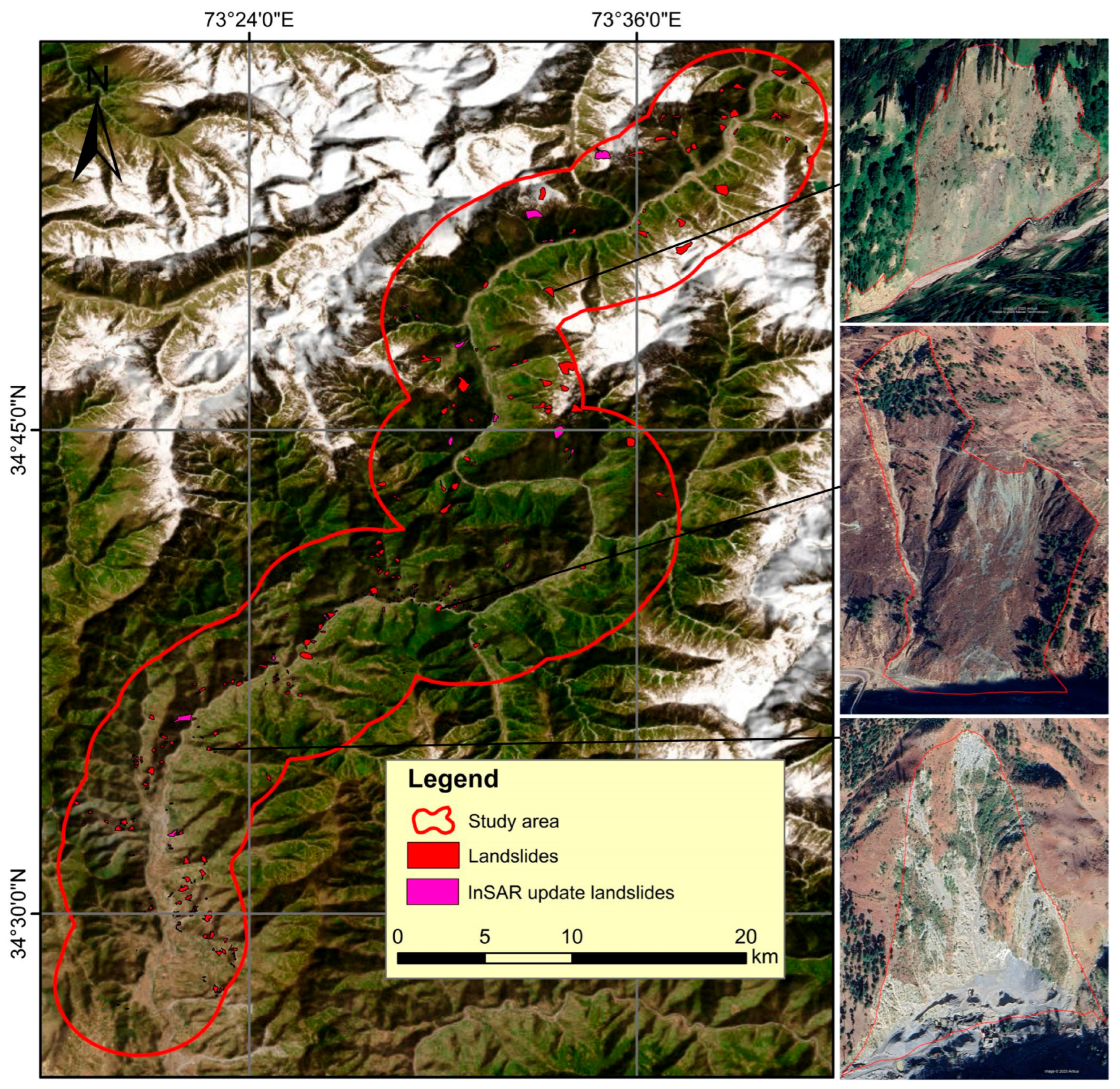
The study area encompasses 102 km of the N-15 highway, which crosses multiple cities. For this study, a buffer zone of approximately 664 km2 was delineated along the 102 km Balakot–Naran highway section using a 5 km Euclidean distance on each side of the road, with the final area smaller than the theoretical ~1020 km2 due to the irregular buffer shape determined by the terrain (Figure 1). In addition to being an alternative to the Karakoram Highway (KKH), this route is also a popular tourist corridor connecting Naran and nearby areas. The scenic corridor between Mansehra and Chilas stretches 240 km and is essential in promoting tourism. The rugged terrain in elevation ranges from 793 to 4360 m above sea level. Subtropical climate prevails in Balakot, whereas alpine climate prevails in Naran, characterized by glaciers and persistent snow cover from October to April. In July and September, the monsoon season dominates the climate [48]. Statistical data from Pakistan’s Meteorological Department (https://www.pmd.gov.pk) indicate annual mean temperatures range from 16.8 °C to 27.3 °C (accessed on 10 February 2023), and annual precipitation averages 670 mm. Tectonic activity and complex geological settings characterize the Balakot–Naran corridor. There are three types of soil in this region: Eutric Cambisols, Lithosols, and Glaciers. It is mainly the Khunar River that runs through this study area. There is a diversity of rock types in the research area [49], including the Tanawal Formation and Manglaur Formation, Sawat and Mansehra Granite complexes, Paleocene and Eocene rocks, Murree Formation, Mesozoic rocks, Korara Complex and Gandaf Formations, and Quaternary Alluvium. Active faults, thrust faults, and suture zones make up the fault system in the study area. Landslides may occur in the lower portions of the region due to the interaction of geological factors like lithology and slope gradient, as well as shifting precipitation patterns and human activity.
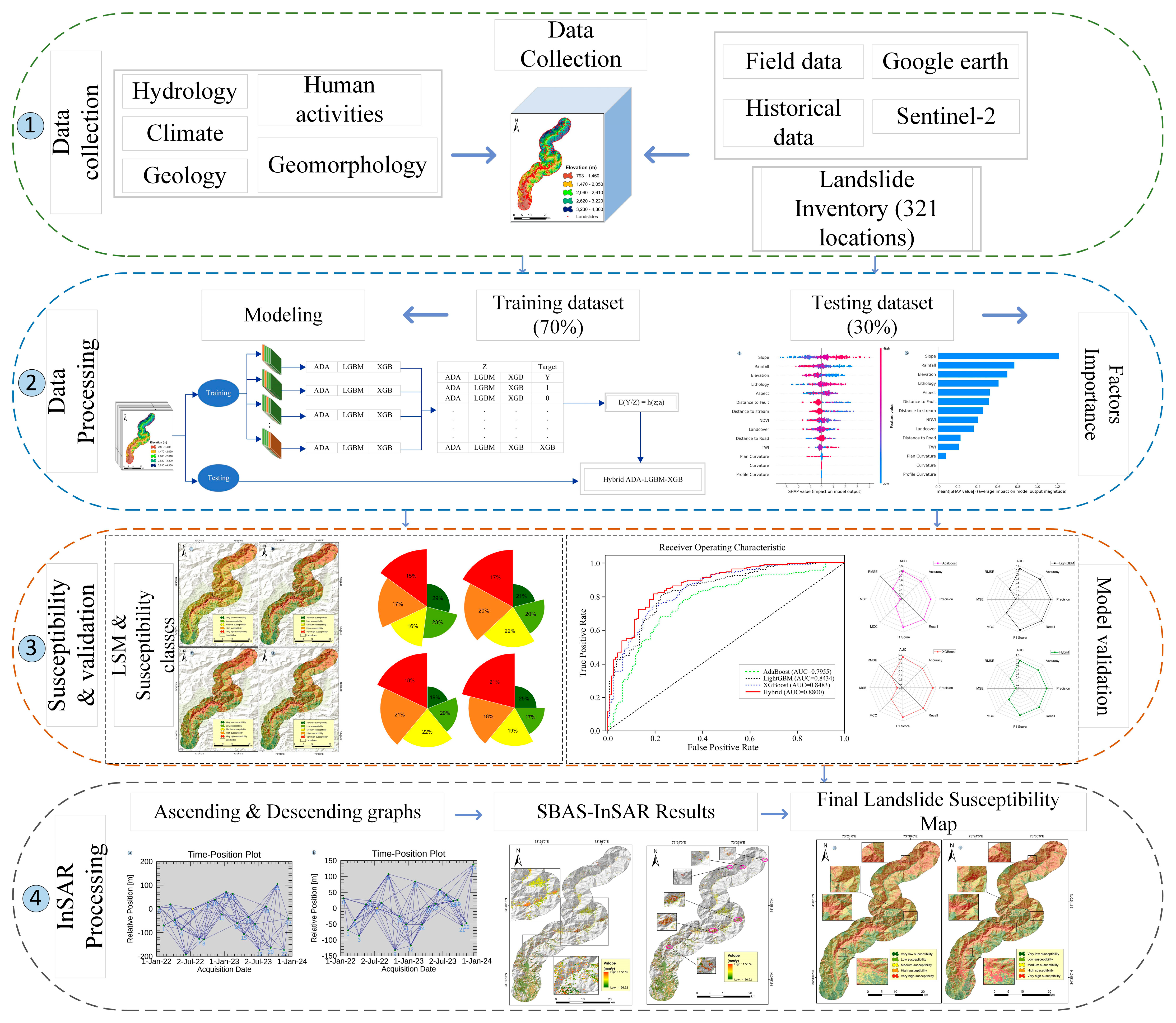
Four main steps were involved in the evaluation process: (1) collecting data, compiling the landslide inventory, and developing LCFs; (2) preparing training and testing datasets; (3) constructing the landslide susceptibility map (LSM), along with comparing and validating all models; and (4) integrating SBAS-InSAR results to generate the enhanced final LSM (Figure 2).

2.2. Landslide Inventory Map

An important component of landslide susceptibility mapping (LSM) is landslide inventory mapping [50]. Landslide inventories play a fundamental role in estimating susceptibility because they provide detailed information on the types of landslides that have historically occurred in the study area. Inventory reliability and accuracy play an important role in the reliability of an LSM [51]. Based on satellite imagery, historical reports, comprehensive field assessments, Google Earth data, and SBAS-InSAR measurements of slope-parallel deformation (Vslope), landslide inventory maps were developed. Sentinel-2 (2023) satellite imagery and Google Earth imagery, together with SBAS-InSAR Vslope maps, contributed to the robustness and reliability of the inventory by supporting comprehensive observations and ensuring data validation. SBAS-InSAR line-of-sight time series were processed and projected to Vslope, and areas exhibiting coherent deformation consistent with geomorphic evidence were used to update the optical inventory by refining polygon boundaries, merging/splitting adjacent features, and flagging previously unmapped active zones; features lacking coherent deformation were deprioritized rather than automatically removed. We used ascending and descending stacks for coherent Vslope clusters and cross-checked each cluster against high-resolution optical imagery and field notes. Clusters showing concordant geomorphic signatures (e.g., head scarps, displaced/accumulated material, vegetation disturbance, or road-cut failures) were incorporated as “SBAS-updated” polygons. Clusters lacking geomorphic corroboration were retained as “candidates” for follow-up and were not labeled as landslides. Through the use of previously documented records and reports, the generated map was cross-verified. A total of 321 landslides covering a cumulative area of 10.82 km2 were identified and digitized using GIS tools (ArcGIS software 10.8), and the datasets were divided randomly into training (70%, 225 landslides) and testing (30%, 96 landslides) (Figure 3). Among these, 50 landslides were directly confirmed through field surveys using handheld GPS and photographic documentation during site visits. The remaining landslides were validated indirectly by cross-checking with high-resolution Google Earth imagery, Sentinel-2 optical data, and previously published reports. Validation criteria included the presence of clear geomorphic signatures such as displaced material, head scarps, and vegetation disturbance, combined with spatial consistency across multiple data sources. This multi-source verification approach ensured both spatial completeness and reliability of the inventory. Additionally, ArcGIS software 10.8was used to extract the centroids of landslide polygons for accurate spatial representation. Landslide data can be simplified by using this approach, which is widely adopted in LSM studies [52]. This method can minimize potential variability in influencing factors within landslide boundaries [53]. There are several types of landslides mapped in the research area, including debris flows, rockfalls, and scree slopes. To illustrate typical landslide features, three representative sites were selected as inset maps (Figure 3). These sites were chosen because they represent different types of landslides observed along the corridor and were cross-verified using high-resolution imagery.

2.3. Landslide Conditioning Factors (LCFs)

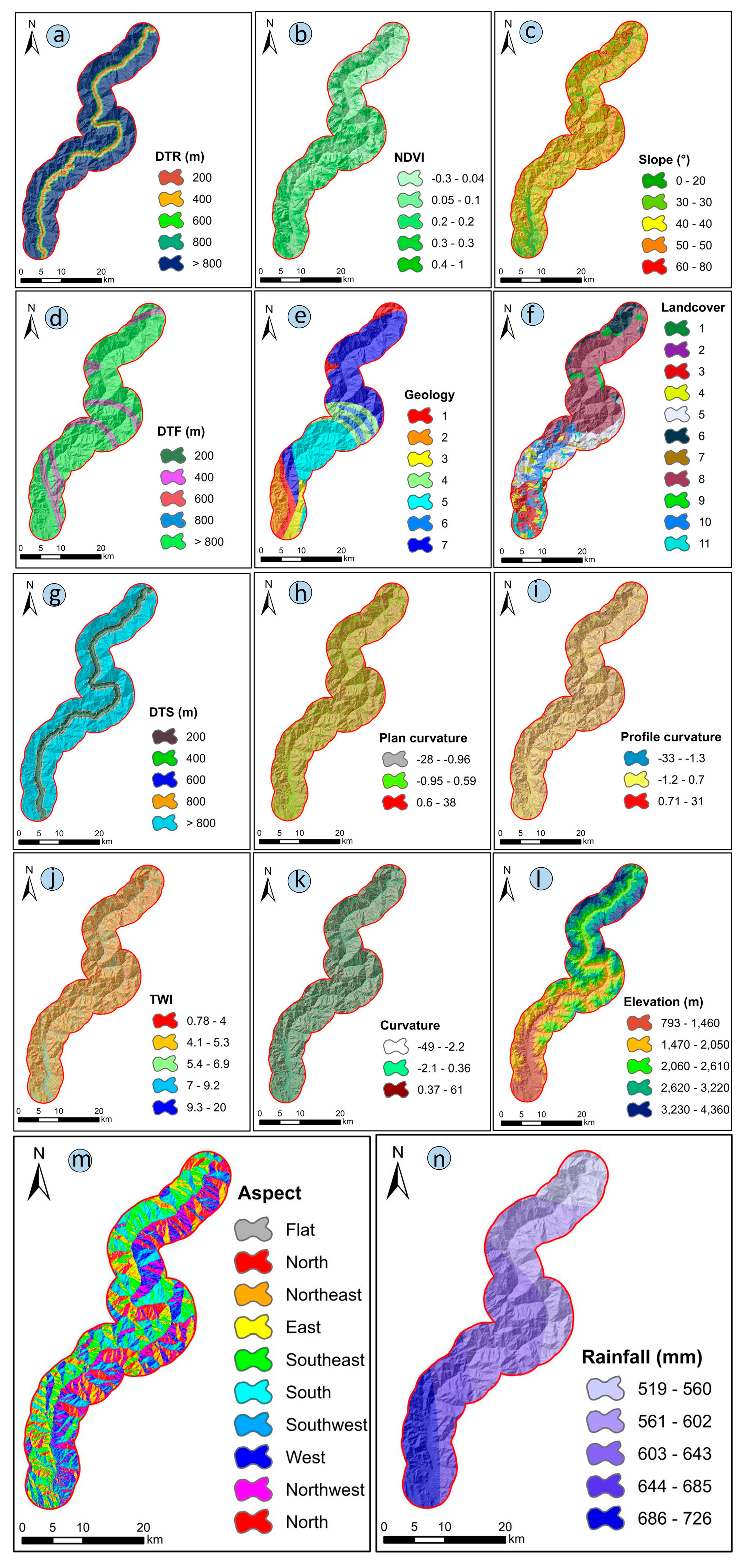
Landslide susceptibility modeling requires careful selection and preparation of the LCF database [30]. Based on recent research into landslide susceptibility and the availability of relevant data for the study area, and since LSM does not follow a consistent standard for determining independent factors [54], the factors used in this study were selected in accordance with a review of recent landslide susceptibility research [55]. An analysis of 14 causative factors was conducted, as shown in Table 1 and Figure 4. These parameters are as follows: distance to road (m), normalized difference vegetation index (NDVI), slope (°), distance to faults (m), geology, landcover, distance to stream (m), plan curvature, profile curvature, topographic wetness index (TWI), curvature, elevation (m), aspect, and rainfall (mm). Based on ALOS-PALSAR DEMs with a spatial resolution of 12.5 m, topographic factors were derived. Sentinel-2 imagery with a 10-m resolution was used to obtain landcover and NDVI data. A lower NDVI is indicative of a higher likelihood of landslides, according to Sajid et al. [56]. A 1:500,000 scale geological map was used to generate spatial maps of distance to faults and geology (via buffering). The LSM uses a standard grid cell model since it is often used for spatial visualization and analysis [55]. Given that the 14 LCF maps differ in spatial resolution and measurement scales, all maps were resampled to a uniform resolution of 12.5 m × 12.5 m to maintain consistency in further analysis (Table 1). As interdependencies between variables in the training dataset may introduce noise that reduces model accuracy in landslide susceptibility assessments, the appropriate assortment of factors is crucial [47]. This study used Shapley Additive Explanations (SHAP) and Recursive Feature Elimination (RFE) for feature selection and assessed multicollinearity using a mixed-association matrix (|Spearman’s ρ| for continuous–continuous, Cramér’s V for categorical–categorical pairs, and correlation ratio η for continuous–categorical).
Landslide and non-landslide samples are essential for generating landslide susceptibility maps using data mining techniques [55]. It is generally agreed that non-landslide data are far more valuable than landslide data, even if the complete landslide dataset is used [57]. To conduct this study, 225 landslide locations (70%) were sequentially selected for training, while 96 locations (30%) were selected for validation. To construct the absence dataset, an equal number of non-landslide samples (321) were generated to balance the presence data. These absence points were systematically extracted from areas outside the mapped landslide polygons, with a minimum buffer distance of 200 m to avoid edge misclassification. Additional constraints were applied by excluding steep slopes (>45°), riverbeds, glaciers, and urbanized zones to reduce false negatives. The final balanced dataset (321 landslides + 321 non-landslides) was randomly split into training (70%) and testing (30%) subsets for model development. The next step was to extract 14 landslide conditioning factors (LCFs) from both landslide and non-landslide samples, thereby forming the basis for the training and validation datasets.

2.4. Modeling

2.4.1. Adaptive Boosting (AdaBoost)

In ensemble learning, Adaptive Boosting (AdaBoost) is one of the most advanced algorithms [58]. A more accurate and robust prediction model is constructed by combining multiple weak classifiers. The fundamental concept involves training a number of classifiers on the same dataset and then integrating them to form a more powerful classifier. Boosting involves iteratively generating multiple individual classifiers, beginning with a decision tree-based model trained on a subset of the dataset. AdaBoost increases the weights applied to misclassified samples with each iteration, thus prioritizing these more difficult cases in subsequent rounds. A model is initially trained with equal weights for all samples; however, as the training progresses, the algorithm places greater emphasis on the misclassified samples. Based on all decision tree classifiers developed during the iterative process, the final predictive model is constructed. With this approach, AdaBoost is able to progressively minimize overall model error and improve prediction accuracy [59].

2.4.2. Light Gradient Boosting (LightGBM)

LightGBM integrates decision trees and boosting in a gradient learning algorithm. This is the first comprehensive discussion of it due to its relatively recent development [60]. LightGBM uses a leaf-wise algorithm for growing vertically, which makes it different from XGBoost. LightGBM uses histogram-based algorithms to accelerate training, reduce memory usage, and apply a leaf-wise growth strategy constrained by depth, which sets it apart from others. The method consists of designing a histogram with bins of k based on continuous floating-point eigenvalues. As opposed to conventional algorithms that require extra storage for presorted results, LightGBM stores feature values after discretization, typically as eight-bit integers, which reduces memory consumption by an eighth. There is no compromise in the accuracy of the model as a result of this coarse classification.

2.4.3. Extreme Gradient Boosting (XGBoost)

Gradient Tree Boosting is a powerful ML technique developed by Chen and Guestrin (2016) that is built into the XGBoost supervised classification model [61]. In addition to being designed for training with multiple processing cores, XGBoost can also capture and learn nonlinear data patterns. As compared to standard boosting techniques, it minimizes overfitting and enhances model precision by using regularized boosting [62]. Scalability across a variety of use cases with minimal computational resources is provided by XGBoost, along with high performance (i.e., speed), capability to handle sparse data, and ease of implementation [63]. A key factor in XGBoost’s success is its additive training approach, which has contributed to its success in numerous data science contests. Model preview settings for the XGBoost model include three primary hyperparameters: nrounds (maximum number of training iterations), subsamples (number of training instances per subsample), and colsample bytree (number of columns to subsample when constructing each tree).

2.4.4. Hybrid (ADA + LGBM + XGB)

In order to construct the hybrid model, we developed a super-learner ensemble that systematically incorporates independent models using the learning algorithms ADABoost, LightGBM, and XGBoost. Initially, the dataset was split into training (Dtrain, 70%) and testing (Dtest, 30%) subsets. Dtrain was further partitioned into Dtrain-train and Dtrain-valid for validation purposes. Hyperparameter optimization for each individual model was carried out using Optuna. The search space for ADABoost, LightGBM, and XGBoost was defined, and an Optuna study object was initialized for each model. During each trial, hyperparameters were sampled and used to train the models on Dtrain-train, followed by evaluation on Dtrain-valid to compute log-loss. The best-performing hyperparameters, determined by minimum log-loss, were then selected to retrain the models on the full Dtrain.
In the prediction phase, probability outputs (PADA, PLGB, PXGB) for each base model were obtained on the Dtest dataset. A hybrid probability output, Phybrid, was calculated using a weighted combination of these individual probabilities, optimized by minimizing the overall log-loss function:
L α , β , γ = L o g L o s s ( α P A D A + β P L G B + γ P X G B )
The optimal weights (α*, β*, γ*) were determined using a numerical optimizer and subsequently used to compute Phybrid. Finally, the performance of Phybrid was evaluated using a comprehensive set of metrics: AUROC, accuracy, precision, recall, F-measure, MCC, MSE, and RMSE, to assess the effectiveness of the hybrid ensemble in classification tasks. The tenfold cross-validation technique was used to eliminate overfitting and minimize model uncertainties, and then the most effective hyperparameters were identified using a grid-based approach. Complete mathematical formulations for all learners (AdaBoost, XGBoost, LightGBM) and the hybrid, together with metric definitions and the training protocol, are as follows:
Setting and Notation
Training pairs ( x i , y i ) i = 1 N with yi ∈ {0,1}. Let σ(z) = 1/(1 + e−z) denote the logistic function and 1[·] the indicator. Probabilities are reported for class y = 1.
AdaBoost (Binary)
Map labels to ỹi = 2yi − 1 ∈ {−1, +1}. Initialize sample weights D1(i) = 1/N. For rounds t = 1,…,T, the following is performed:
(1)
Fit a weak classifier ht(x) ∈ {−1, +1} on weighted data Dt.
(2)
Weighted error ε t = i = 1 N D t ( i ) 1 [ y ~ i h t ( x i ) ] ( 0 < ε t < 0.5 ) , with 0 < ε_t < 0.5.
(3)
Learner weight α t = 1 2 l n 1 ε t ε t .
(4)
Update and renormalize:
Dt+1(i) ∝ Dt(i) exp{ −αti ht(xi)}.
Final score F(x) = ΣTt=1 αt ht(x);
probability:
p(y = 1|x) = σ(2F(x))
Gradient Boosting Trees
We learn an additive model of regression trees:
f M ( x ) = m = 1 M η b m ( x )
By minimizing the logistic loss,
L = i = 1 N l ( y i , f ( x i ) ) , l ( y , f ) = y l o g p ( 1 y ) l o g ( 1 p ) , p = σ ( f ) .
At stage m (second-order/“Newton” boosting),
p i = σ f m 1 x i , g i = p i y i , h i = p i ( 1 p i )
Fit a tree bm to negative gradients (or use (gi, hi) for Newton step), and then update
f m x = f m 1 x + η b m ( x )
LightGBM specifics: Histogram-based split finding with leaf-wise growth (depth constraints), Gradient-based One-Side Sampling (GOSS), and Exclusive Feature Bundling (EFB) to accelerate training while retaining accuracy. Split gain for a node with left/right children:
G a i n = 1 2 ( G L 2 H L + λ + G R 2 H R + λ G 2 H + λ ) γ
where G = Σ gi and H = Σ hi within the node, and λ, γ are regularization terms.
XGBoost (Regularized Second-Order Boosting)
Objective with tree-level regularization:
L = i = 1 N l y i , y i + m = 1 M Ω T m , Ω ( T ) = γ # l e a v e s ( + λ 2 j w j 2 )
With leaf index q(x) and leaf scores w, the second-order approximation gives the following:
L ~ = j ( G j w j + 1 2 ( H j + λ ) w j 2 ) + γ # l e a v e s , G j = i : q ( x i ) = j g i , H j = i : q ( x i ) = j h i
Optimal leaf weight:
w j = G j H j + λ
Split gain for a node partitioned into left/right children:
G a i n = 1 2 ( G L 2 H L + λ + G R 2 H R + λ G 2 H + λ ) γ
Predicted probability:
p y = 1 x = σ ( f M ( x ) )
Hybrid Ensemble (Soft Voting)
Let pk(y = 1|x) be calibrated probabilities from k ∈ {AdaBoost, LightGBM, XGBoost}. With non-negative, normalized weights Σkwk = 1,
p h y b ( y = 1 x ) = k w k p k ( y = 1 x ) , y ^ = 1 [ p h y b 0.5 ]
Unless stated otherwise, we use equal weights; weight tuning by CV log-loss gave similar results.

2.5. Key Indicators of Landslide Conditioning Factors

2.5.1. Recursive Feature Elimination and Multicollinearity Analysis

Machine learning algorithms are made more efficient by identifying a subset of essential features via the Recursive Feature Elimination (RFE) algorithm. It is common for machine learning algorithms to consume a significant amount of memory and to be highly complex in terms of time, both of which can be mitigated by applying an RFE algorithm. Furthermore, irrelevant features may lead to poor predictive performance when learned algorithms are misled by irrelevant features. Feature selection by RFE is a wrapper-type process that is guided by a machine learning algorithm at its core. It is described as a wrapper-style algorithm because it determines features through a filtering approach. Configuring RFE involves two primary parameters: selecting features and determining the algorithm to be used for evaluating them. Iteratively, each less important feature is removed from the complete set of features until the required number of features is reached. In this process, the core model is fitted, features are ranked by importance, the least significant ones are eliminated, and the model is then re-fitted. In this study, RFE used a Random Forest classifier (500 trees, balanced classes) under 5 × 3 stratified cross-validation; we also computed a selection frequency across folds. The final subset was chosen at the mean-AUROC optimum (ties resolved by F1, and then MCC).
To guard against biased or unstable rankings from multicollinearity, we computed a mixed-association matrix among the 14 LCFs: Spearman’s Ρ for continuous–continuous pairs, the correlation ratio η for continuous–categorical pairs (lithology, landcover), and Cramér’s V for categorical–categorical pairs. We flagged strong association at |Ρ| ≥ 0.80 or η/V ≥ 0.50. Where redundancy was detected (e.g., among curvature metrics or TWI with curvature/slope), we retained the variable with higher cross-validated RFE contribution and clearer physical interpretability and excluded the rest. The optimized set was then used in training and in the Full-14 vs. reduced-feature ablation.

2.5.2. Shapley Additive Explanations (SHAP)

During the early stages of the development of cooperative games, Lee and Lundberg [64] proposed that SHAP values are derived from cooperative game theory, which aims to quantify the contributions of individual players. There have been various techniques developed over the last decade to improve the interpretation of ML models, notably SHAP [65,66] and local model-agnostic explanations [67]. A critical variable, such as slope and rainfall, is better understood through SHAP in landslide prediction. The SHAP algorithm ensures that the cumulative impact of all features is fairly distributed in proportion to their influence by quantifying the individual contribution of each feature to the overall prediction [64], adhering to principles such as uniformity, null effect, and local precision [64]. Three key properties must be present for Shapley values to be computed: local precision, missingness, and robustness [68]. It is the dependence on local features that determines an explanation’s accuracy; missingness measures the variability of the explanation from one instance to another, while robustness measures its consistency with the predictions of the model [69]. A mean marginal contribution is calculated across all possible feature combinations according to Shapley’s framework:
i = S N S ! n S 1 ! n ! v S i v ( S ) ]
Here, i denotes the significance of a feature i, N represents the set of all variables, n is the quantity of variables in N, S is a subset of N not including i, and v(N) represents the base value corresponding to the estimated result for N without accounting for particular variable values.

2.6. Model Evaluation and Validation

Landslide susceptibility models need to be validated and their accuracy assessed, as, without proper validation, any model’s scientific credibility is undermined [70]. As part of this study, ROCs and overall accuracy (OA) were used to determine the efficiency of the developed framework [71]. When the area under the curve (AUC) value is close to 1, the prediction method is assumed to be effective [72,73]. To assess binary classifications, Matthew’s correlation coefficient (MCC) was also applied, even in significantly imbalanced classes [74]. When the MCC value is 1, it indicates perfect prediction; when it is 0 or −1, it represents random calculation and an obvious contradiction between prediction and observation.
In order to evaluate the forecasting capability of landslide forecasts, statistical measurements such as precision, AUROC, F1-measure, MSE, MCC, and RMSE were applied. These statistical measurements were calculated using the subsequent formulas [75]:
A c c u r a c y = ( T P + T N ) / ( T P + F P + T N + F N )
S e n s i t i v i t y = T P / ( T P + F N )
S p e c i f i c i t y = T N / ( T N + F P )
A U R O C = ( T P + T N ) / ( P + N ) .
F 1 m e a s u r e = 2 T P / ( 2 T P + F P + F N )
P r e c i s i o n = T P / ( T P + F P )
M C C = ( T P × T N F P × F N ) / ( ( T P + F P ) ( T P + F N ) ( T N + F P ) ( T N + F N ) )
M S E = 1 n y i y i ^ 2
R M S E = s q r t M S E = s a r t ( ( 1 n y i y i ^ 2 ) )

2.7. SBAS-InSAR

The small baseline subset (SBAS) technology uses the same principles as the Persistent Scatterer Interferometry (PSI) technique originally developed by Ferretti [76]. As opposed to PSI, which uses single-master interferograms, SBAS uses multi-master interferogram pairs for its deformation analysis, resulting in more interferograms within the same monitoring period. Compared to PSI, SBAS models unwrap and difference interferograms, solving the deformation signals using the Singular Value Decomposition [77] method. It applies spatial–temporal unwrapping to small baseline pairs over distributed targets, whereas PSI performs phase unwrapping (or integer-ambiguity estimation) on a sparse network of persistent scatterers while jointly estimating deformation rate, residual topography, and atmospheric components. Spatial decorrelation is effectively mitigated by SBAS when all available interferogram pairs with small baselines are combined efficiently. SAR images can be more effectively utilized when isolated interferogram subsets are integrated, thus improving temporal resolution and maximizing the utilization of each image. Consequently, SBAS delivers more reliable results for geophysical research by providing continuous spatial deformation fields [76].
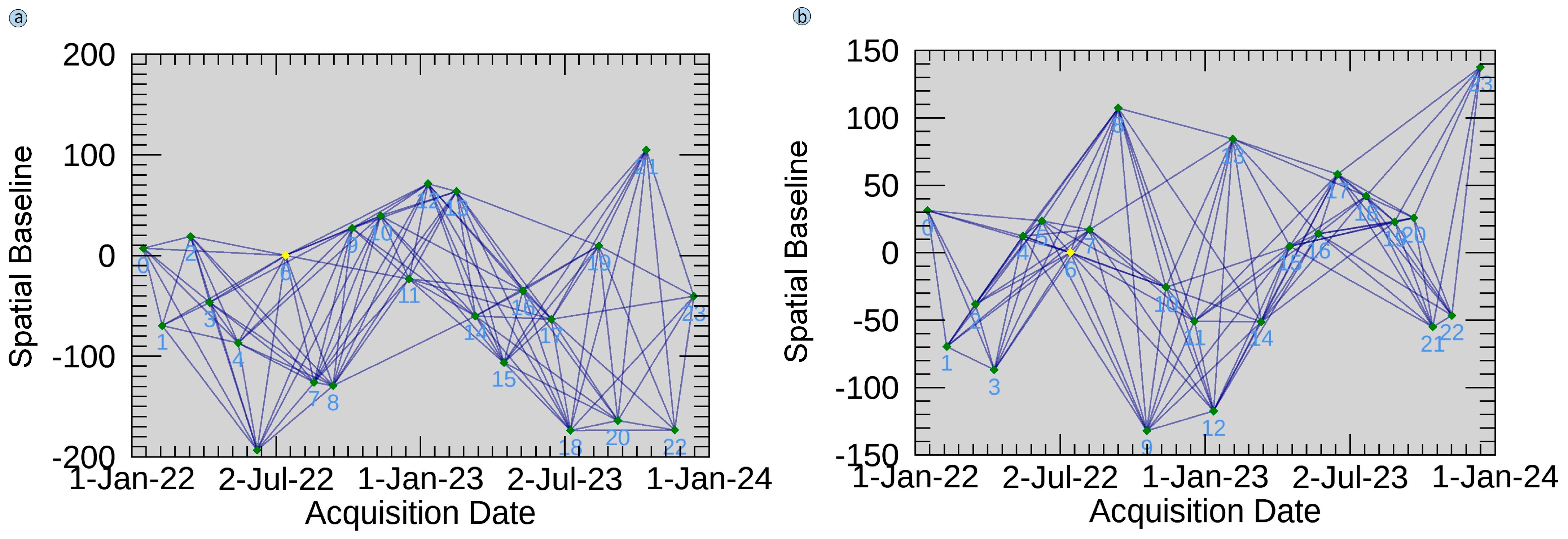
ENVI version 5.6.3 was used for SBAS-InSAR processing in this study. Unless otherwise specified, velocities were reported in the line-of-sight (LOS) direction (positive toward the sensor) and were additionally projected onto the local slope-parallel direction (Vslope) for geomorphic interpretation. Ascending and descending stacks were processed independently. A connection graph was generated as the first step. As a result, 532 interferogram pairs were generated using 110-m spatial baselines and 90-day temporal baselines (Figure 5). An important step in interferogram processing is the use of a Goldstein filter, which enhances both phase unwrapping and measurement accuracy, maximizing the signal-to-noise ratio [78]. In order to unwrap phases, the Minimum Cost Flow [79] was used with a coherence threshold of 0.35. Thus, unwrapping errors were excluded from the connection graph for interferogram pairs with low coherence. Interferograms that were not refined or re-flattened using GCPs were then refined and re-flattened using Ground Control Points. To qualify for GCPs, they needed to be located in stable, nondeforming regions and within well-unwrapped phases. They were required to have coherence values exceeding 0.7 [80] in order to ensure the accuracy of GCPs. Long-wavelength orbital ramps were removed by fitting a 2D planar surface to each interferogram (least squares on coherent pixels); the stratified tropospheric delay was modeled as an elevation-dependent phase term (tile-based fit using the DEM); and residual atmospheric phase screens were mitigated with the standard SBAS temporal high-pass/spatial low-pass filtering (spatial low-pass = 1000 m; temporal high-pass = 365 days) prior to SVD inversion. A DEM-error term proportional to the perpendicular (spatial) baseline was jointly estimated and removed. The time series in each track were referenced to a stable patch (γ ≥ 0.70). Deformation was then solved via SVD on the unwrapped, differenced interferograms. Based on 48 images acquired from 2022 to 2023, the SAR dataset consists primarily of ascending and descending scenes (Table 2).
Surface deformations along the LOS are measured by the SBAS method. Mountainous areas do not exhibit sufficient deformation in the LOS direction to accurately reflect slope deformation. Using the formulas below, the deformation rate along the slope is transformed to the deformation rate along the LOS path.
V s l o p e = V L O S c o s
I n d e x = n l o s × n s l o p e
n l o s = s i n θ c o s α s , s i n θ s i n α s , c o s θ
n s l o p e = ( s i n α · c o s φ ,                 c o s α · c o s φ , s i n φ )
In this context, Vslope represents the deformation rate along the slope angle, while Vlos denotes the deformation rate in the line-of-sight (LOS) orientation. Here, α is the aspect, θ is the radar incidence angle, φ is the slope, and αs is the angle between the satellite orbit direction and true north. For the data convention, values from ascending passes are negative, whereas those from descending passes are positive.

3. Results

3.1. RFE Technique and Multicollinearity Analysis

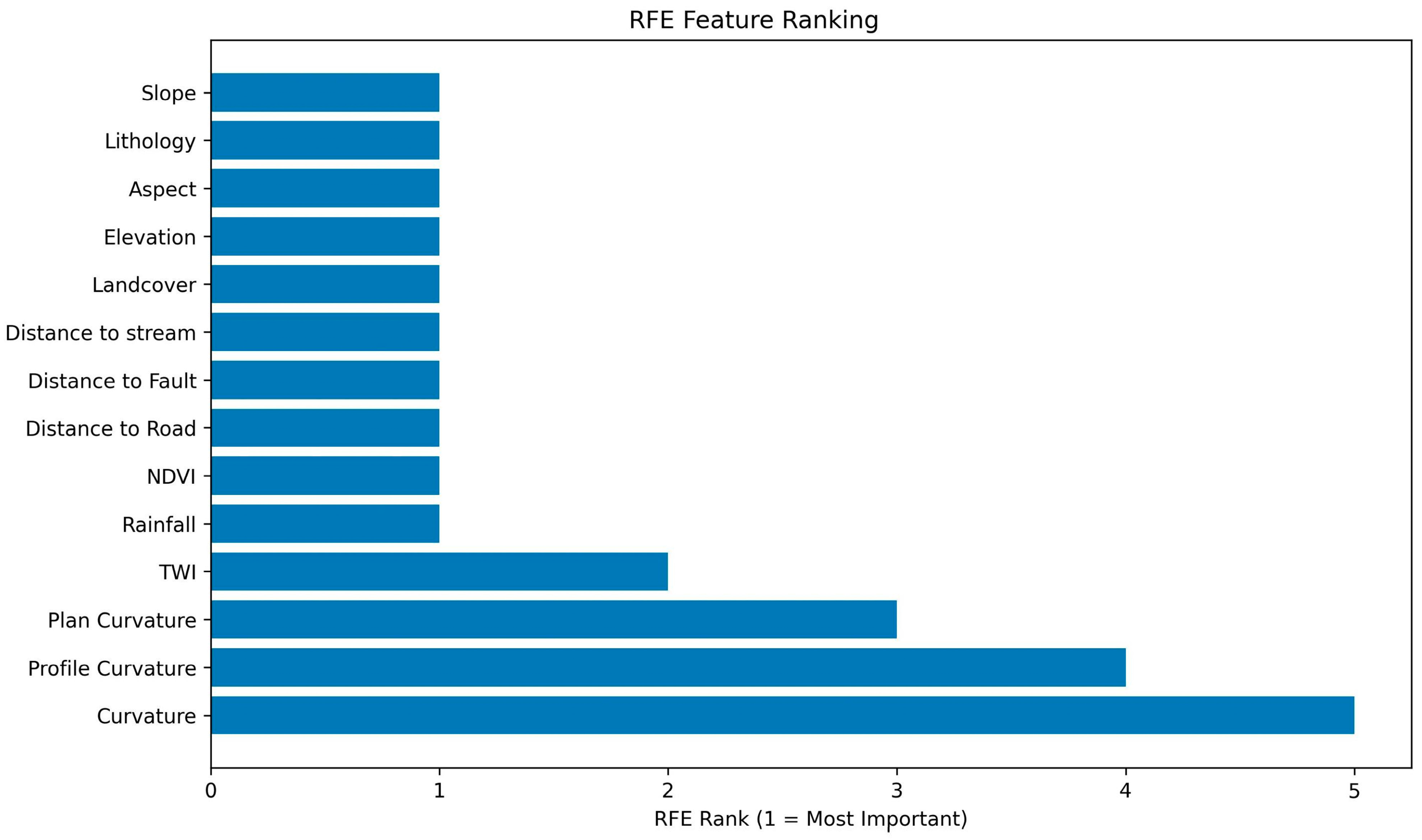
A Recursive Feature Elimination algorithm (RFE) was used to rank and choose the most relevant landslide susceptibility factors (Figure 6). In addition to ordinal ranks, we report normalized Random Forest importance weights and selection frequency (Table 3). At the accuracy-optimal subset (n = 10), the RFE-retained features (rank = 1) were slope, aspect, lithology, NDVI, landcover, elevation, rainfall, distance to fault, distance to stream, and distance to road. Collectively, these ten predictors accounted for 94% of the total importance (sum of weights = 0.94); the top five (Slope, Aspect, Lithology, NDVI, Landcover) alone contributed 0.58. Distance to road showed slightly lower stability (selection frequency = 0.83), and TWI, although physically relevant, was not consistently selected (RFE rank = 2; selection frequency = 0.17). Curvature-derived variables (plan, profile, overall curvature) showed negligible quantitative contributions (combined weight = 0.02) and were not retained in repeated RFE (selection frequency = 0), indicating limited standalone predictive power. For landslide susceptibility analyses, RFE simplified the model input, improving performance and interpretability.
Figure 7 summarizes pairwise associations among the 14 LCFs (|Spearman’s ρ| for continuous–continuous pairs, Cramér’s V for categorical–categorical, and correlation ratio η for continuous–categorical). A strong correlated block is evident among plan curvature, profile curvature, and curvature; TWI shows moderate association with curvature/slope. The three distance variables (stream/road/fault) are at most moderately associated with one another and are weakly associated with the remaining predictors. Lithology and landcover display low–moderate associations with rainfall/elevation, reflecting broad environmental gradients rather than duplication. Apart from the curvature cluster (and TWI), most pairs are <0.5, indicating limited multicollinearity. This pattern corroborates the SHAP/RFE outcome, in which the curvature metrics and TWI were deprioritized, and supports the use of the optimized 10-factor subset in the final models.

3.2. Shapley Additive Explanations (SHAP) Value

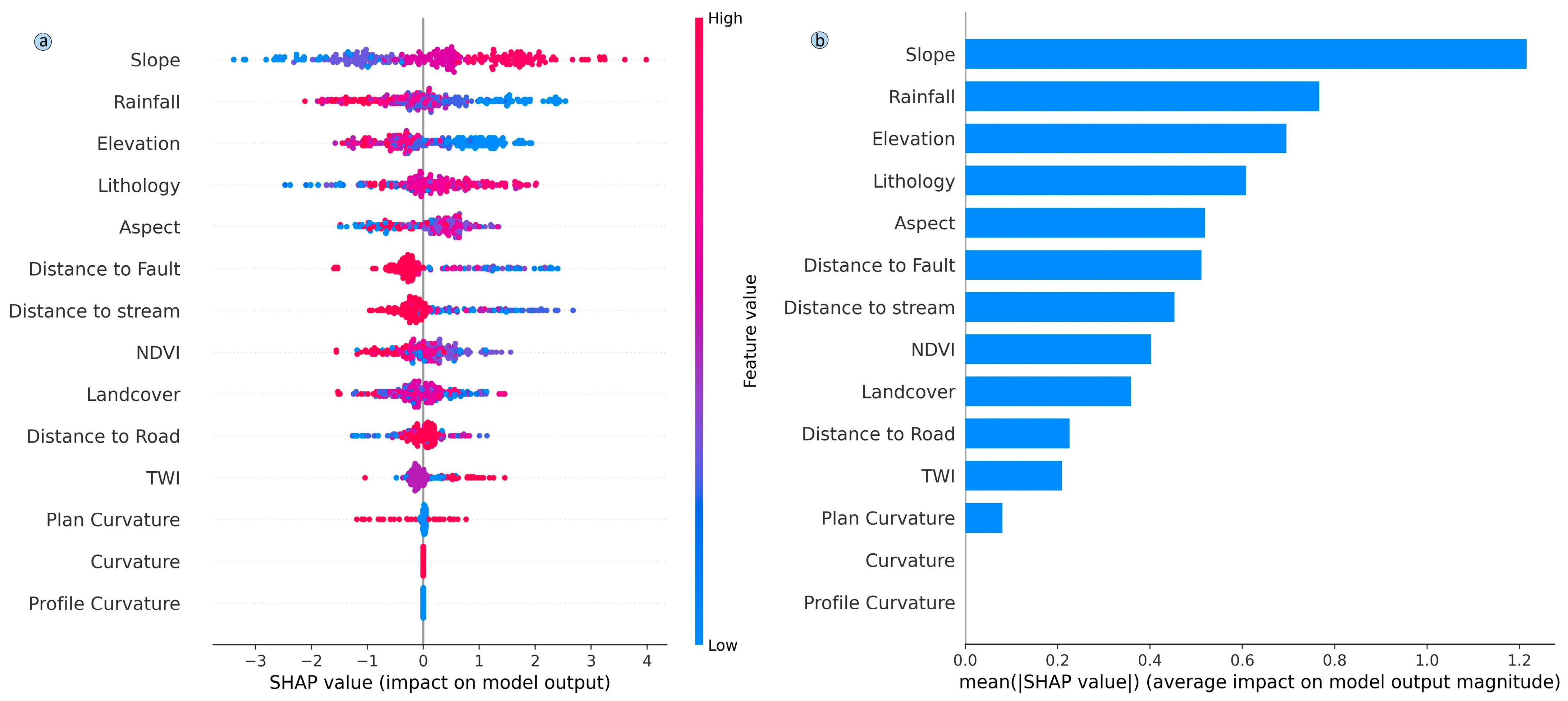
In data-driven modeling, SHAP coefficient diagrams and correlation plots are used to illustrate the dynamic relationship between contributing variables and landslide susceptibility [81]. Landslides are less likely to occur when SHAP values are negative, while they are more likely to occur when SHAP values are positive. Landslide susceptibility is computed using SHAP values, indicated on the x-axis. Using a blue-to-red color gradient, the parameter values are visualized with blue representing low values and red representing high values, facilitating the visualization of how the intensity of individual variables impacts the model. The precision and reliability of the susceptibility assessment model can be compromised by redundant factors. In order to mitigate these adverse effects, factor optimization has been shown to be effective [82]. Using Shapley values as a measure of each variable’s contribution to the model’s performance, this study quantifies each variable’s predictive power. Based on the Shapley model, the influencing factors are ranked according to their importance, as illustrated in Figure 8a. SHAP values for each conditioning factor are plotted on a horizontal axis, with blue values indicating less than zero and red values indicating greater than zero. Landslide susceptibility is most strongly affected by slope when its values are low, whereas rainfall is most influential when its values are high. Figure 8b further investigates the relative contributions of each factor, indicating that slope has the most substantive influence on the model (+0.99), followed by rainfall (+0.80), while curvature influences the least (+0.02).
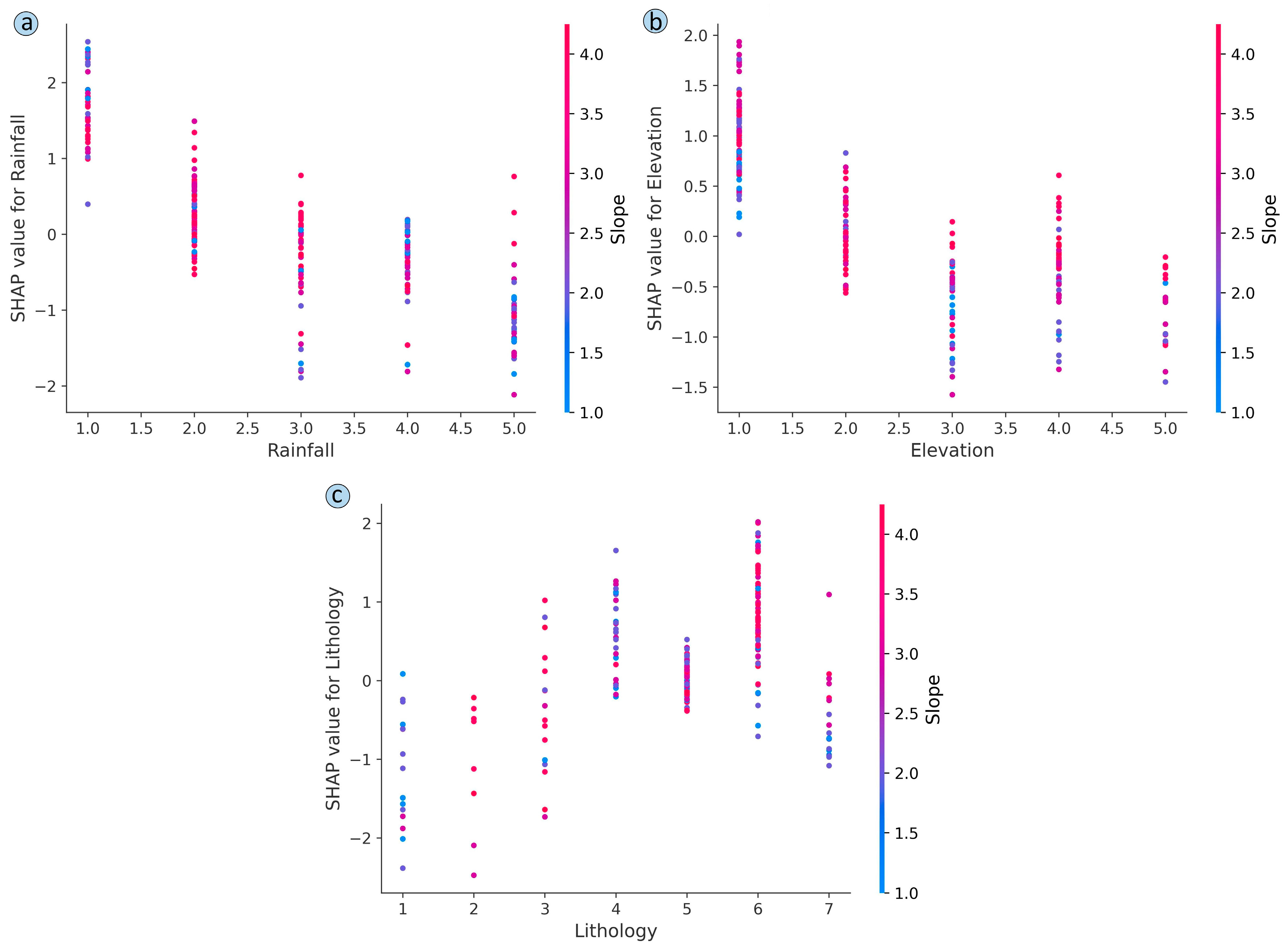
The correlation plot serves two objectives: (1) observing the contribution of a single variable to model predictions and (2) analyzing the significance of the relationships between two variables [83,84]. In order to determine the most significant variables affecting landslides, correlation plots and two-factor relationship plots were developed. A two-factor dependence plot was constructed by comparing slope with another important factor (Figure 9).

3.3. Landslide Susceptibility Mapping

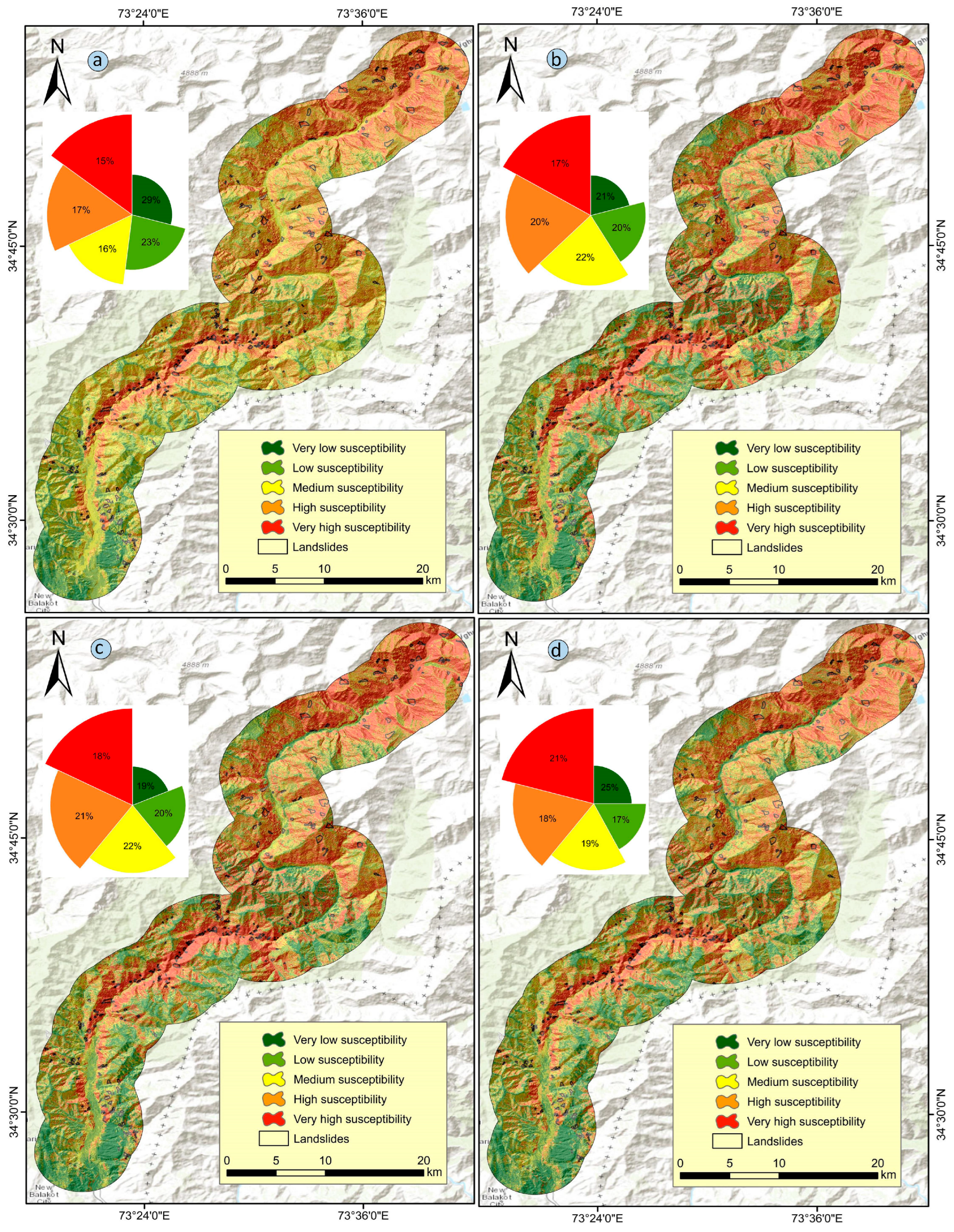
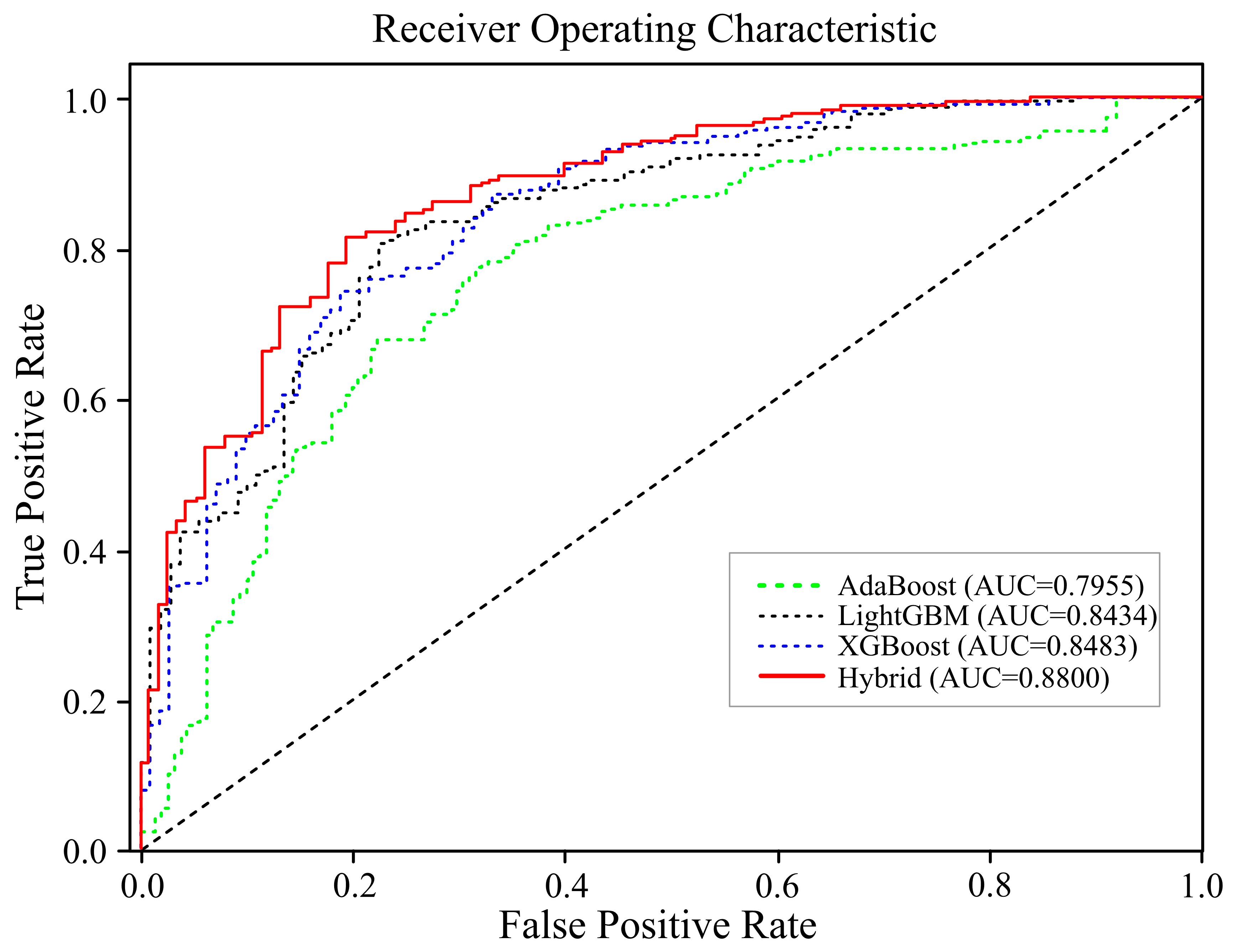
Landslide susceptibility maps (LSMs) were developed using machine learning models: AdaBoost, LightGBM, XGBoost, and a hybrid model composed of ADA + LGBM + XGB (Figure 10). Experimental results indicated that the hybrid model outperformed the individual models in terms of overall accuracy. The LSMs were classified into five susceptibility categories using the Jenks natural break method [85] in ArcGIS. The very high susceptibility areas for AdaBoost, LightGBM, XGBoost, and hybrid are 15%, 17%, 18%, and 21%, respectively. High- and moderate-susceptibility areas for AdaBoost, LightGBM, XGBoost, and hybrid are 17%, 20%, 21%, 18% and 16%, 22%, 22%, and 19%, respectively. The values for very low and low susceptibility for the four models are 29%, 21%, 19%, and 25% and 23%, 20%, 20%, and 17%, respectively. According to the results, each model exhibits a comprehensive distribution of susceptibility across all classes, as illustrated in Figure 10. An ROC [86] technique, which plots sensitivity against specificity across various threshold levels, was used to further validate the model. The AUC (area under the curve) of the ROC was used to quantitatively assess model performance [87]. The AUC values for AdaBoost, LightGBM, XGBoost, and the hybrid model were 79.55%, 84.34%, 84.83%, and 88.00%, respectively (Figure 11), demonstrating the hybrid ensemble’s superior predictive ability.
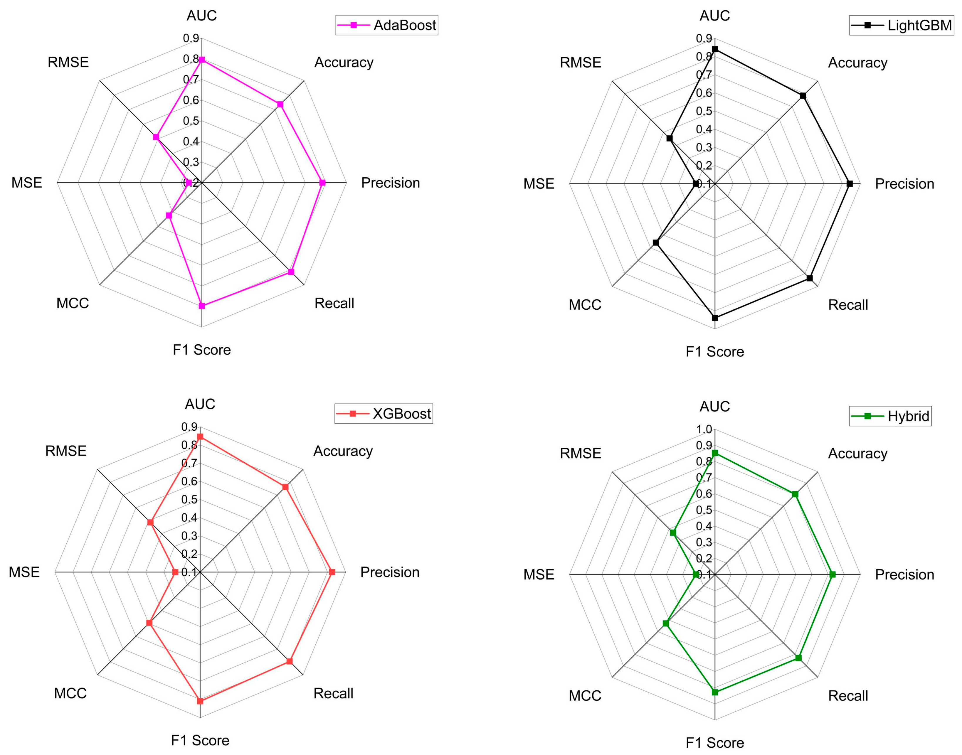
To quantify the effect of feature selection, we trained each model with the full set of 14 LCFs and with the RFE-10 subset (distance to road, NDVI, slope, distance to faults, geology, landcover, distance to stream, elevation, aspect, rainfall) using identical splits in stratified 10-fold cross-validation. For each setting, we report the fold-averaged AUROC, accuracy, precision, recall, F1 score, MSE, MCC, and RMSE (Table 4); thresholded metrics used a 0.5 cutoff on the probability outputs. Relative to Full-14, RFE-10 improved performance for all models, with the largest gains for the hybrid (AUROC 83.66 to 88.00; accuracy 77.27 to 80.52; F1 82.05 to 84.69; MCC 51.09 to 57.90; RMSE 47.67 to 44.13). XGBoost also improved (81.92 to 84.83 AUROC), while AdaBoost and LightGBM showed modest but positive changes (78.72 to 79.55 and 84.00 to 84.34 AUROC, respectively). These results indicate that removing redundant factors enhances generalization without sacrificing accuracy; we therefore adopt RFE-10 for subsequent mapping and analysis. On the basis of tenfold cross-validation, average values were calculated for various evaluation metrics, including AUC, precision, accuracy, F1-score, recall, MCC, RMSE, and MSE. Further visualization of these statistics was provided by radar charts (Figure 12).

3.4. SBAS-InSAR Results

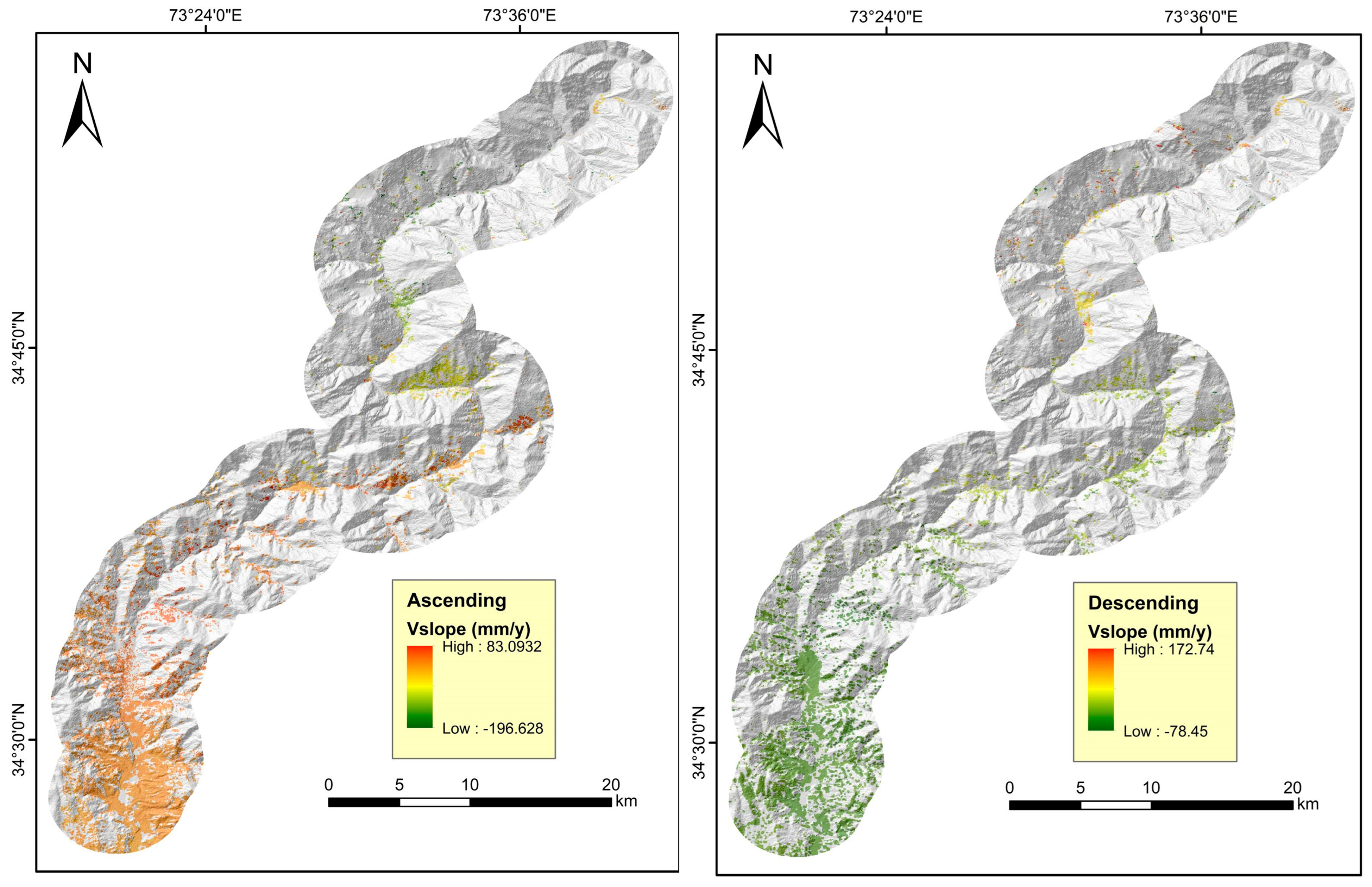
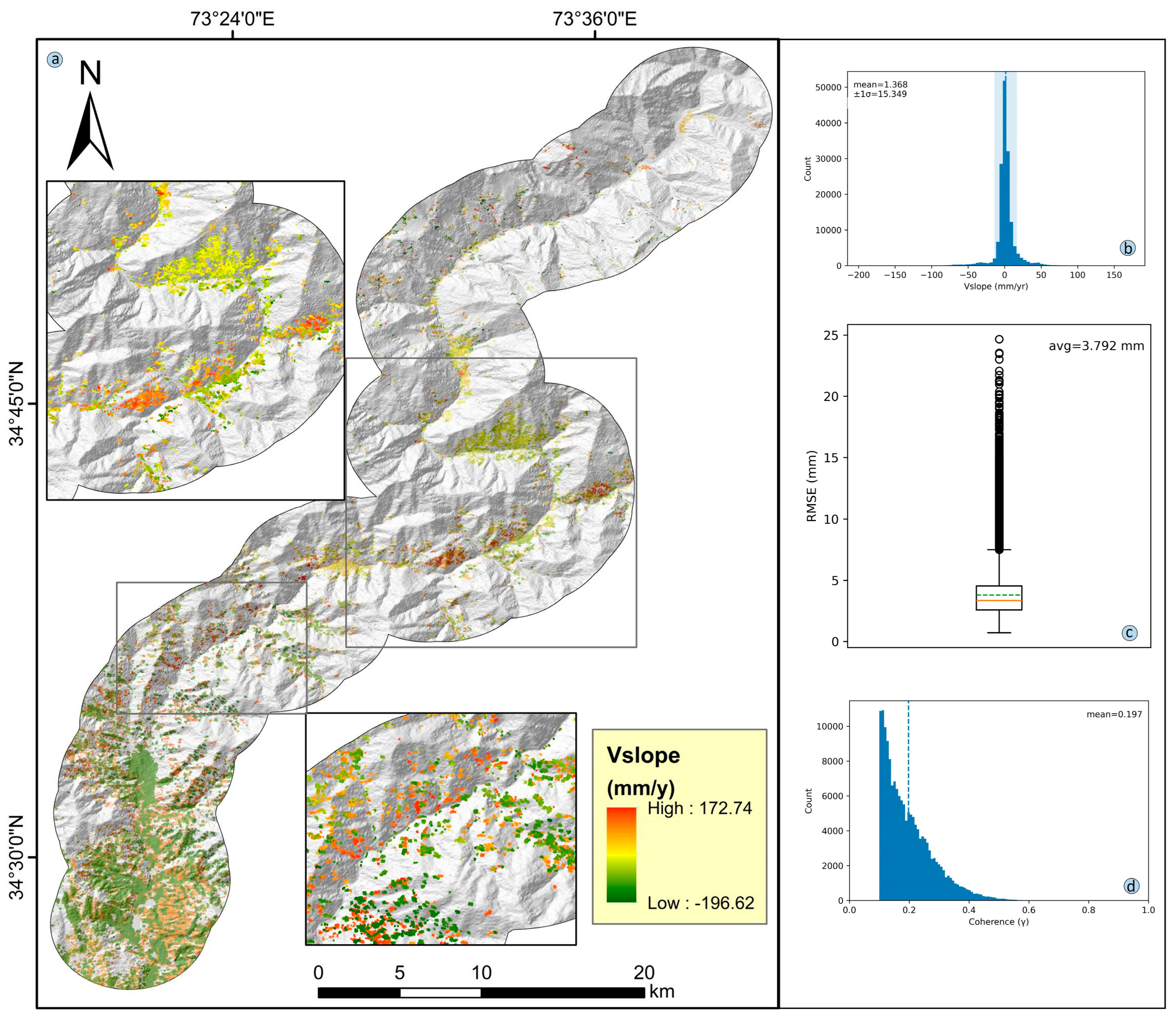
This study used SBAS-InSAR to process SAR data consisting of 48 scenes acquired between 2022 and 2023. A connectivity map is generated in SARscape, and the super-master image is automatically selected. Inversion and geocoding were performed after interferometric processing to determine displacement velocity. Data quality was ensured by applying a coherence threshold of 0.7. Geocoding was used to calculate displacement velocity along slope direction in the research area (Figure 13). There were a range of velocity values ranging from −196.629 mm per year to 172.74 mm per year (Figure 14a, ascending and descending), with a mean displacement of 1.368 mm per year and a standard deviation of 15.349 mm per year (Figure 14b). The average root mean square error (RMSE) was 3.792 mm, while the mean coherence value was 0.197 (Figure 14c,d). Localized, coherent deformation was detected in several zones. Where kinematic anomalies aligned with geomorphic evidence, we updated the inventory (SBAS-updated polygons); other anomalies are retained as candidates pending validation.
Figure 13. SBAS-InSAR results in the research area from ascending and descending.
Remotesensing 17 03464 g013
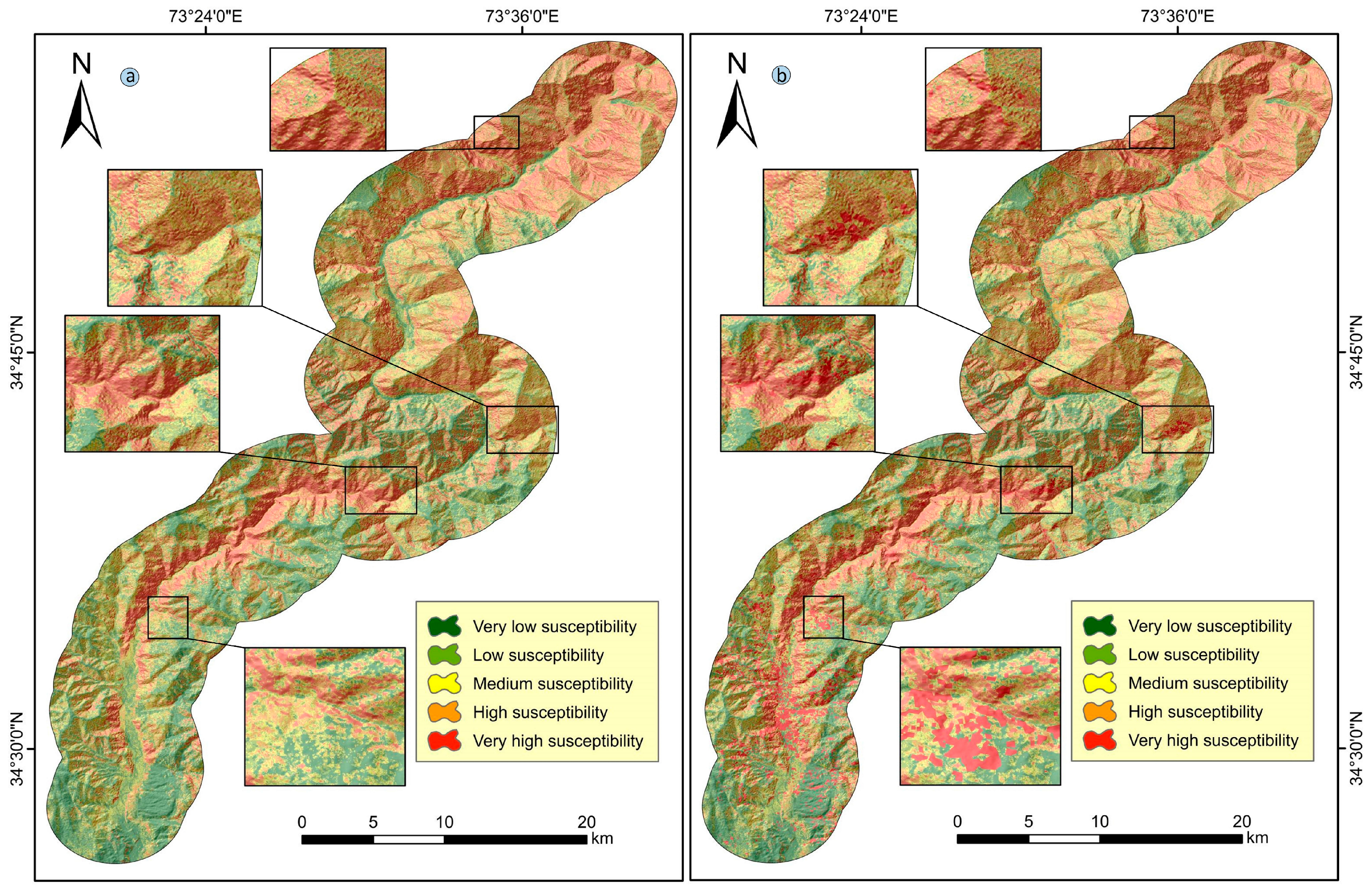
Figure 14. SBAS-InSAR results. (a) Displacement velocity along the slope (ascending and descending), (b) Vslope distribution with mean and ±1 σ, (c) interferogram RMSE (mm) shown as a boxplot with the average annotated, and (d) coherence (γ) distribution with mean value; the blue dashed vertical line marks the mean coherence. The final landslide susceptibility map (LSM) was generated through an integration of the predictive outcomes of the SBAS-InSAR Vslope deformation and the hybrid model outputs. The hybrid model exhibited instances of misclassification and omission in several regions, particularly in regions categorized as very high and high susceptibility. This assessment was based on a pixel-wise overlay between the susceptibility map and two independent references—the 321-site inventory and coherent SBAS-InSAR clusters—where “omission” denotes inventoried or coherently deforming sites lying in low/moderate classes, and “misclassification” denotes high/very high pixels lacking both inventory evidence and a coherent Vslope cluster (activity thresholds: Vslope ≥ 10 mm per yr; γ ≥ 0.35). A more detailed LSM aligned with the hybrid model’s output was generated by resampling the Vslope into 12.5 × 12.5 m grid cells. LSM refinement for the study area relied on a contingency matrix crossing Vslope activity with the five susceptibility classes (Figure 15). We then compared the hybrid map and the refined LSM on a cell-by-cell basis to quantify differences. In summary, the integration of SBAS-InSAR-results enhanced the final LSM spatial comprehensiveness and reliability significantly.
Remotesensing 17 03464 g014
Figure 15. Refined LSM for the study area. (a) Hybrid LSM; (b) newly integrated LSM.
Remotesensing 17 03464 g015

4. Discussion

In this study, slope-parallel displacement velocity data from both descending and ascending SBAS-InSAR datasets were analyzed in conjunction with optical remote sensing imagery and field observations to determine the preliminary landslide boundaries. A digital elevation model (DEM) was analyzed for topographic features, and optical images were examined for patterns in areas experiencing relatively high deformation velocities. This SBAS-InSAR analysis led to the detection and mapping of numerous previously unidentified potential landslides (Figure 16). A zone with a high or very high susceptibility to landslides is likely to be in a zone with a high likelihood of landslides. It is noteworthy that several of these zones are absent from the landslide inventory compiled in this research, suggesting that they are likely to be high-risk regions for landslides in the future. Therefore, we recommend that continuous monitoring be carried out in these areas and that timely preventive measures be taken to mitigate any possible landslide hazards.
As a result of the integration of SBAS-InSAR with slope deformation velocity (Vslope), the landslide inventory has been enhanced to detect slow-moving landslides and identify previously undocumented events. The use of SBAS-InSAR not only updated the inventory but also improved the reliability of LSM through the correction of misclassifications and identification of active deformation zones. There has been an increasing emphasis on temporal deformation integration in the recent literature to overcome the limitations of traditional inventories [38,39]. SBAS-InSAR’s capability to capture linear as well as nonlinear deformations makes it especially useful in terrains like Balakot–Naran, where landslides are induced both by human activities and natural processes. The findings are consistent with previous InSAR-based studies [54,88], which transformed LOS displacement rates into slope-parallel displacements to assess landslide activity more accurately.
A comparative analysis of AdaBoost, LightGBM, and XGBoost machine learning classifiers, as well as the hybrid model (ADA + LGBM + XGB), demonstrated the robust predictive capabilities of ensemble learning methods in LSM. The hybrid model had the highest area under the curve (AUC = 0.88) and also exhibited superior precision, recall, and F1-scores, indicating its optimal balance between sensitivity and specificity. According to recent studies, combining individual models reduces overfitting, improves generalization, and improves overall performance in LSM challenges [89,90]. Compared to single models, the hybrid model’s advantage lies in its potential to integrate the strengths of each component: AdaBoost’s effectiveness on hard-to-classify instances, LightGBM’s performance in handling large-scale data with its leaf-wise splitting approach, and XGBoost’s robust regularization to minimize overfitting. These findings are consistent with ensemble-based approaches that have been used for geohazard assessments [89,91,92].
In this study, machine learning models provided more accurate classifications and spatial differentiation than conventional statistical and bivariate methods previously used in the region. Logistic regression and frequency ratio methods have been widely used in Pakistan’s mountainous regions [93,94], but they have limitations when it comes to capturing nonlinear relationships between LCFs. By using a hybrid ensemble approach, this study overcomes these limitations and provides a reproducible, scalable model suitable for other high-risk areas. Furthermore, previous studies have rarely integrated deformation data directly into models. There is no previous study that has integrated SBAS-InSAR-derived Vslope data with ML classifiers for LSM in the Balakot region, filling an important gap both in the existing geohazard literature and in model optimization methodologies in this region.
A Recursive Feature Elimination (RFE) and Shapley Additive Explanations (SHAP) analysis determined slope, elevation, lithology, aspect, and landcover as the primary influential variables in landslide occurrence. The importance of slope and elevation is consistent with the complexity of the topography in the study region, where steep slopes and high altitudes contribute to gravitational instabilities. In tectonically active and high-relief regions [95,96,97], slope gradient and elevation have also been found to be primary factors in triggering landslides. In particular, weathered rocks and unconsolidated Quaternary deposits have been noted to significantly affect slope stability due to geology. Several geological units in the Himalayan foothills, including the Murree Formation and Tanawal Formation, are often found in landslide-prone zones, which is similar to previous research [37]. Through its effect on solar radiation and snowmelt patterns, aspect also influences soil moisture and vegetation cover, both of which are crucial to regulating slope hydrology. Rainfall and NDVI were moderately important, consistent with studies showing that areas with sparse vegetation and high rainfall tend to be more prone to landslides [98,99]. Curvature-related variables, in contrast, ranked lower, indicating they contributed less to model complexity and refinement, though their inclusion increased model complexity.

Future Directions

The study acknowledges several limitations despite the improved performance. It is difficult to detect landslides at a detailed spatial or temporal level due to a lack of high-resolution temporal data. Additionally, some model misclassifications may be caused by variables that are not included in the LCFs, such as underground water flow or seismic activity. Lastly, even though the hybrid model shows better performance, it is computationally intensive and may need to be optimized for real-time hazard monitoring. A future study should include data on rainfall thresholds and soil moisture sensors. InSAR and ML models may further enhance future LSM spatial precision and inventory completeness when LIDAR- and UAV-derived datasets are integrated with them. The generalizability and practicality of this hybrid approach can also be validated by applying it to broader regions and temporal scales.

5. Conclusions

A comprehensive and integrated approach to landslide susceptibility mapping (LSM) along the Balakot–Naran route is presented in this study. AdaBoost, LightGBM, XGBoost, and a hybrid ensemble model are used along with SBAS-InSAR-derived slope deformation data to develop an enhanced landslide susceptibility map. Among all models, the hybrid classifier demonstrated superior predictive performance, achieving the highest AUC, accuracy, precision, and F1-score, confirming ensemble learning’s ability to capture complex nonlinear relationships between landslides and conditioning factors. In this research, fourteen landslide conditioning factors were used, with slope, elevation, lithology, landcover, and aspect being identified as the most influential factors via a Recursive Feature Elimination and Shapley Additive Explanations model. Through the integration of SBAS-InSAR, the LSM was able to detect active slope deformation and correct misclassifications. It also enhances the spatial precision and accuracy of landslide susceptibility outputs by reducing the gap between past occurrences and current slope instability. As a result, the final susceptibility maps help policymakers, urban planners, and disaster risk managers identify high-risk zones, prioritize mitigation strategies, and develop infrastructure accordingly. It will be helpful to integrate dynamic environmental variables such as rainfall thresholds, soil moisture, and seismicity into future research in order to further refine the model’s robustness and extend its applicability to other regions prone to landslides.

Author Contributions

Conceptualization, I.U.; methodology, I.U.; software, M.A.H.; validation, N.A.; formal analysis, S.U.S.; investigation, M.A.H.; resources, N.A.; data curation, S.U.S.; writing—original draft, I.U.; writing—review and editing, M.A.H.; visualization, I.U.; supervision, Z.C.; project administration, Z.C.; funding acquisition, Z.C. All authors have read and agreed to the published version of the manuscript.

Funding

This research was funded by Deep Earth Probe and Mineral Resources Exploration—National Science and Technology Major Project under Grant 2025ZD1008501; Programs National Natural Science Foundation of China (42471475); the Opening Fund of Key Laboratory of Geological Survey and Evaluation of Ministry of Education (Grant No. GLAB 2024ZR06).

Data Availability Statement

Data will be made available on request to the first author and corresponding author.

Conflicts of Interest

The authors declare no conflicts of interest.

References

  1. Liu, T.; Liu, Y.; Zhang, C.; Yuan, L.; Sui, X.; Chen, Q. Hyperspectral image super-resolution via dual-domain network based on hybrid convolution. IEEE Trans. Geosci. Remote Sens. 2024, 62, 5512518. [Google Scholar] [CrossRef]
  2. Yang, Z.Q.; Zhu, Y.Y.; Zou, D.S.; Liao, L.P. Activity degree evaluation of glacial debris flow along international Karakorum Highway (KKH) based on fuzzy theory. Adv. Mater. Res. 2011, 261, 1167–1171. [Google Scholar] [CrossRef]
  3. Dey, S.; Das, S.; Roy, S.K. Demystifying the predictive capability of advanced heterogeneous machine learning ensembles for landslide susceptibility assessment and mapping in the Eastern Himalayan Region, India. Nat. Hazards 2025, 121, 13407–13446. [Google Scholar] [CrossRef]
  4. Meena, S.R.; Hussain, M.A.; Ullah, H.; Ullah, I. Landslide susceptibility mapping using hybrid machine learning classifiers: A case study of Neelum Valley, Pakistan. Bull. Eng. Geol. Environ. 2025, 84, 242. [Google Scholar] [CrossRef]
  5. Yang, Z.; Fan, X.; Yang, Y.; Hou, K.; Du, J.; Chen, X.; Mi, Y.; Jiang, C.; Zhang, J.; Guo, Y. Deformation patterns and failure mechanism of high and steep stratified rock slopes with upper steep and lower gentle style induced by step-by-step excavations. Environ. Earth Sci. 2022, 81, 229. [Google Scholar] [CrossRef]
  6. Yang, Z.; Zhao, X.; Chen, M.; Zhang, J.; Yang, Y.; Chen, W.; Bai, X.; Wang, M.; Wu, Q. Characteristics, dynamic analyses and hazard assessment of debris flows in Niumiangou Valley of Wenchuan County. Appl. Sci. 2023, 13, 1161. [Google Scholar] [CrossRef]
  7. Yu, Z.; Ning, Z.; Chang, W.-Y.; Chang, S.J.; Yang, H. Optimal harvest decisions for the management of carbon sequestration forests under price uncertainty and risk preferences. For. Policy Econ. 2023, 151, 102957. [Google Scholar] [CrossRef]
  8. Alcántara-Ayala, I. Landslides in a changing world. Landslides 2025, 22, 2851–2865. [Google Scholar] [CrossRef]
  9. Raihan, A. A comprehensive review of the recent advancement in integrating deep learning with geographic information systems. Res. Briefs Inf. Commun. Technol. Evol. 2023, 9, 98–115. [Google Scholar] [CrossRef]
  10. Zhong, C.; Liu, Y.; Gao, P.; Chen, W.; Li, H.; Hou, Y.; Nuremanguli, T.; Ma, H. Landslide mapping with remote sensing: Challenges and opportunities. Int. J. Remote Sens. 2020, 41, 1555–1581. [Google Scholar] [CrossRef]
  11. Hong, Y.; Adler, R.; Huffman, G. Use of satellite remote sensing data in the mapping of global landslide susceptibility. Nat. Hazards 2007, 43, 245–256. [Google Scholar] [CrossRef]
  12. Ghorbanzadeh, O.; Blaschke, T.; Aryal, J.; Gholaminia, K. A new GIS-based technique using an adaptive neuro-fuzzy inference system for land subsidence susceptibility mapping. J. Spat. Sci. 2020, 65, 401–418. [Google Scholar] [CrossRef]
  13. Sestraș, P.; Bilașco, Ș.; Roșca, S.; Naș, S.; Bondrea, M.V.; Gâlgău, R.; Vereș, I.; Sălăgean, T.; Spalević, V.; Cîmpeanu, S.M. Landslides susceptibility assessment based on GIS statistical bivariate analysis in the hills surrounding a metropolitan area. Sustainability 2019, 11, 1362. [Google Scholar] [CrossRef]
  14. Ding, Q.; Chen, W.; Hong, H. Application of frequency ratio, weights of evidence and evidential belief function models in landslide susceptibility mapping. Geocarto Int. 2017, 32, 619–639. [Google Scholar] [CrossRef]
  15. Youssef, A.M.; Pourghasemi, H.R. Landslide susceptibility mapping using machine learning algorithms and comparison of their performance at Abha Basin, Asir Region, Saudi Arabia. Geosci. Front. 2021, 12, 639–655. [Google Scholar] [CrossRef]
  16. Constantin, M.; Bednarik, M.; Jurchescu, M.C.; Vlaicu, M. Landslide susceptibility assessment using the bivariate statistical analysis and the index of entropy in the Sibiciu Basin (Romania). Environ. Earth Sci. 2011, 63, 397–406. [Google Scholar] [CrossRef]
  17. Habiballah, R.; Witam, O.; Ibnoussina, M. An Ensemble modeling of frequency ratio (FR) with evidence belief function (EBF) for GIS-based landslide susceptibility mapping: A case study of the coastal cliff of Safi, Morocco. J. Indian Soc. Remote Sens. 2023, 51, 2243–2263. [Google Scholar] [CrossRef]
  18. Wang, Y.; Nanehkaran, Y.A. GIS-based fuzzy logic technique for mapping landslide susceptibility analyzing in a coastal soft rock zone. Nat. Hazards 2024, 120, 10889–10921. [Google Scholar] [CrossRef]
  19. Oleng, M.; Ozdemir, Z.; Pilakoutas, K. Co-seismic and rainfall-triggered landslide hazard susceptibility assessment for Uganda derived using fuzzy logic and geospatial modelling techniques. Nat. Hazards 2024, 120, 14049–14082. [Google Scholar] [CrossRef]
  20. Kotzé, J.; Le Roux, J.; van Tol, J. Creating a landslide inventory in the Eastern Cape Province, South Africa: A pixel-based change detection method using fuzzy membership functions. Nat. Hazards 2025, 121, 18249–18274. [Google Scholar] [CrossRef]
  21. Kucuker, D.M. lyzing landslide susceptibility of forest roads by analytical hierarchy process (AHP) in of forest planning unit of Turkiye. Nat. Hazards 2025, 121, 2323–2345. [Google Scholar] [CrossRef]
  22. Chicas, S.D.; Li, H.; Mizoue, N.; Ota, T.; Du, Y.; Somogyvári, M. Landslide susceptibility mapping core-base factors and models’ performance variability: A systematic review. Nat. Hazards 2024, 120, 12573–12593. [Google Scholar] [CrossRef]
  23. Nwazelibe, V.E.; Egbueri, J.C.; Unigwe, C.O.; Agbasi, J.C.; Ayejoto, D.A.; Abba, S.I. GIS-based landslide susceptibility mapping of Western Rwanda: An integrated artificial neural network, frequency ratio, and Shannon entropy approach. Environ. Earth Sci. 2023, 82, 439. [Google Scholar] [CrossRef]
  24. Chen, Y. Spatial prediction and mapping of landslide susceptibility using machine learning models. Nat. Hazards 2025, 121, 8367–8385. [Google Scholar] [CrossRef]
  25. Abdelkader, M.M.; Csámer, Á. Comparative assessment of machine learning models for landslide susceptibility mapping: A focus on validation and accuracy. Nat. Hazards 2025, 121, 10299–10321. [Google Scholar] [CrossRef]
  26. Mao, Y.; Qin, H.; Yaojun, S.; Zilong, H.; Zhaohui, G.; Decheng, M.; Kouhdaragh, M. Implementing an explored advanced and integrated deep random forest learning-based model to monitor the enhanced landslide susceptibility mapping. Nat. Hazards 2025, 121, 15655–15677. [Google Scholar] [CrossRef]
  27. Liu, B.; Guo, H.; Li, J.; Ke, X.; He, X. Application and interpretability of ensemble learning for landslide susceptibility mapping along the Three Gorges Reservoir area, China. Nat. Hazards 2024, 120, 4601–4632. [Google Scholar] [CrossRef]
  28. Nguyen, C.Q.; Nguyen, D.A.; Tran, H.T.; Nguyen, T.T.; Thao, B.T.P.; Cong, N.T.; Van Phong, T.; Van Le, H.; Prakash, I.; Pham, B.T. Predicting landslide and debris flow susceptibility using Logitboost alternating decision trees and ensemble techniques. Nat. Hazards 2025, 121, 1661–1686. [Google Scholar] [CrossRef]
  29. Shang, H.; Liu, S.; Zhong, J.; Tsangaratos, P.; Ilia, I.; Chen, W.; Chen, Y.; Liu, Y. Application of Naive Bayes, kernel logistic regression and alternation decision tree for landslide susceptibility mapping in Pengyang County, China. Nat. Hazards 2024, 120, 12043–12079. [Google Scholar] [CrossRef]
  30. Hussain, M.A.; Chen, Z.; Zhou, Y.; Meena, S.R.; Ali, N.; Shah, S.U. Landslide susceptibility mapping using artificial intelligence models: A case study in the Himalayas. Landslides 2025, 22, 2089–2103. [Google Scholar] [CrossRef]
  31. Pawar, N.S.; Sharma, K.V. Comprehensive review of remote sensing integration with deep learning in landslide forecasting and future directions. Nat. Hazards 2025, 1, 1–35. [Google Scholar] [CrossRef]
  32. Xu, Z.; Che, A.; Zhou, H. Seismic landslide susceptibility assessment using principal component analysis and support vector machine. Sci. Rep. 2024, 14, 3734. [Google Scholar] [CrossRef] [PubMed]
  33. Wu, Y.; Ke, Y.; Chen, Z.; Liang, S.; Zhao, H.; Hong, H. Application of alternating decision tree with AdaBoost and bagging ensembles for landslide susceptibility mapping. Catena 2020, 187, 104396. [Google Scholar] [CrossRef]
  34. Youssef, K.; Shao, K.; Moon, S.; Bouchard, L.-S. Landslide susceptibility modeling by interpretable neural network. Commun. Earth Environ. 2023, 4, 162. [Google Scholar] [CrossRef]
  35. Hussain, M.A.; Chen, Z.; Wang, R.; Shoaib, M. PS-InSAR-based validated landslide susceptibility mapping along Karakorum Highway, Pakistan. Remote Sens. 2021, 13, 4129. [Google Scholar] [CrossRef]
  36. Zhao, F.; Meng, X.; Zhang, Y.; Chen, G.; Su, X.; Yue, D. Landslide susceptibility mapping of Karakorum highway combined with the application of SBAS-InSAR technology. Sensors 2019, 19, 2685. [Google Scholar] [CrossRef] [PubMed]
  37. Rehman, M.U.; Zhang, Y.; Meng, X.; Su, X.; Catani, F.; Rehman, G.; Yue, D.; Khalid, Z.; Ahmad, S.; Ahmad, I. Analysis of landslide movements using interferometric synthetic aperture radar: A case study in Hunza-Nagar Valley, Pakistan. Remote Sens. 2020, 12, 2054. [Google Scholar] [CrossRef]
  38. Oliveira, S.; Zêzere, J.; Catalão, J.; Nico, G. The contribution of PSInSAR interferometry to landslide hazard in weak rock-dominated areas. Landslides 2015, 12, 703–719. [Google Scholar] [CrossRef]
  39. Piacentini, D.; Devoto, S.; Mantovani, M.; Pasuto, A.; Prampolini, M.; Soldati, M. Landslide susceptibility modeling assisted by Persistent Scatterers Interferometry (PSI): An example from the northwestern coast of Malta. Nat. Hazards 2015, 78, 681–697. [Google Scholar] [CrossRef]
  40. Berardino, P.; Fornaro, G.; Lanari, R.; Sansosti, E. A new algorithm for surface deformation monitoring based on small baseline differential SAR interferograms. IEEE Trans. Geosci. Remote Sens. 2002, 40, 2375–2383. [Google Scholar] [CrossRef]
  41. Lanari, R.; Mora, O.; Manunta, M.; Mallorquí, J.J.; Berardino, P.; Sansosti, E. A small-baseline approach for investigating deformations on full-resolution differential SAR interferograms. IEEE Trans. Geosci. Remote Sens. 2004, 42, 1377–1386. [Google Scholar] [CrossRef]
  42. Zhang, Y.; Meng, X.; Jordan, C.; Novellino, A.; Dijkstra, T.; Chen, G. Investigating slow-moving landslides in the Zhouqu region of China using InSAR time series. Landslides 2018, 15, 1299–1315. [Google Scholar] [CrossRef]
  43. Shrestha, M.; Sharma, S.; Pradhan Shrestha, R. Landslides in the Himalayas: A Comprehensive Review of Hazards, Impacts, and Adaptive Strategies. Rural Reg. Dev. 2025, 3, 10002. [Google Scholar] [CrossRef]
  44. Roy, J.; Saha, S.; Arabameri, A.; Blaschke, T.; Bui, D.T. A novel ensemble approach for landslide susceptibility mapping (LSM) in Darjeeling and Kalimpong districts, West Bengal, India. Remote Sens. 2019, 11, 2866. [Google Scholar] [CrossRef]
  45. Hong, H.; Pradhan, B.; Xu, C.; Bui, D.T. Spatial prediction of landslide hazard at the Yihuang area (China) using two-class kernel logistic regression, alternating decision tree and support vector machines. Catena 2015, 133, 266–281. [Google Scholar] [CrossRef]
  46. Kavzoglu, T.; Sahin, E.K.; Colkesen, I. Landslide susceptibility mapping using GIS-based multi-criteria decision analysis, support vector machines, and logistic regression. Landslides 2014, 11, 425–439. [Google Scholar] [CrossRef]
  47. Tien Bui, D.; Ho, T.-C.; Pradhan, B.; Pham, B.-T.; Nhu, V.-H.; Revhaug, I. GIS-based modeling of rainfall-induced landslides using data mining-based functional trees classifier with AdaBoost, Bagging, and MultiBoost ensemble frameworks. Environ. Earth Sci. 2016, 75, 1101. [Google Scholar] [CrossRef]
  48. Khan, S.F.; Kamp, U.; Owen, L.A. Documenting five years of landsliding after the 2005 Kashmir earthquake, using repeat photography. Geomorphology 2013, 197, 45–55. [Google Scholar] [CrossRef]
  49. Searle, M.; Khan, M.A.; Fraser, J.; Gough, S.; Jan, M.Q. The tectonic evolution of the Kohistan-Karakoram collision belt along the Karakoram Highway transect, north Pakistan. Tectonics 1999, 18, 929–949. [Google Scholar] [CrossRef]
  50. Guzzetti, F.; Carrara, A.; Cardinali, M.; Reichenbach, P. Landslide hazard evaluation: A review of current techniques and their application in a multi-scale study, Central Italy. Geomorphology 1999, 31, 181–216. [Google Scholar] [CrossRef]
  51. Abbas, H.; Hussain, D.; Khan, G.; ul Hassan, S.N.; Kulsoom, I.; Hussain, S. Landslide Inventory and Landslide Susceptibility Mapping for China Pakistan Economic Corridor (CPEC)’s main route (Karakorum Highway). J. Appl. Emerg. Sci. 2021, 11, 18–30. [Google Scholar]
  52. Jacobs, L.; Dewitte, O.; Poesen, J.; Maes, J.; Mertens, K.; Sekajugo, J.; Kervyn, M. Landslide characteristics and spatial distribution in the Rwenzori Mountains, Uganda. J. Afr. Earth Sci. 2017, 134, 917–930. [Google Scholar] [CrossRef]
  53. Zêzere, J.; Pereira, S.; Melo, R.; Oliveira, S.; Garcia, R.A. Mapping landslide susceptibility using data-driven methods. Sci. Total Environ. 2017, 589, 250–267. [Google Scholar] [CrossRef] [PubMed]
  54. Hussain, M.A.; Chen, Z.; Zheng, Y.; Zhou, Y.; Daud, H. Deep learning and machine learning models for landslide susceptibility mapping with remote sensing data. Remote Sens. 2023, 15, 4703. [Google Scholar] [CrossRef]
  55. Tsangaratos, P.; Ilia, I. Comparison of a logistic regression and Naïve Bayes classifier in landslide susceptibility assessments: The influence of models complexity and training dataset size. Catena 2016, 145, 164–179. [Google Scholar] [CrossRef]
  56. Sajid, T.; Maimoon, S.K.; Waseem, M.; Ahmed, S.; Khan, M.A.; Tränckner, J.; Pasha, G.A.; Hamidifar, H.; Skoulikaris, C. Integrated Risk Assessment of Floods and Landslides in Kohistan, Pakistan. Sustainability 2025, 17, 3331. [Google Scholar] [CrossRef]
  57. Dahal, R.K.; Hasegawa, S.; Nonomura, A.; Yamanaka, M.; Dhakal, S.; Paudyal, P. Predictive modelling of rainfall-induced landslide hazard in the Lesser Himalaya of Nepal based on weights-of-evidence. Geomorphology 2008, 102, 496–510. [Google Scholar] [CrossRef]
  58. He, Q.; Jiang, Z.; Wang, M.; Liu, K. Landslide and wildfire susceptibility assessment in Southeast Asia using ensemble machine learning methods. Remote Sens. 2021, 13, 1572. [Google Scholar] [CrossRef]
  59. Pham, B.T.; Bui, D.T.; Prakash, I.; Dholakia, M. Hybrid integration of Multilayer Perceptron Neural Networks and machine learning ensembles for landslide susceptibility assessment at Himalayan area (India) using GIS. Catena 2017, 149, 52–63. [Google Scholar] [CrossRef]
  60. Ke, G.; Meng, Q.; Finley, T.; Wang, T.; Chen, W.; Ma, W.; Ye, Q.; Liu, T.-Y. LightGBM: A highly efficient gradient boosting decision tree. In Proceedings of the 31st International Conference on Neural Information Processing Systems, Long Beach, CA, USA, 4–9 December 2017; pp. 3149–3157. [Google Scholar]
  61. Ma, B.; Meng, F.; Yan, G.; Yan, H.; Chai, B.; Song, F. Diagnostic classification of cancers using extreme gradient boosting algorithm and multi-omics data. Comput. Biol. Med. 2020, 121, 103761. [Google Scholar] [CrossRef] [PubMed]
  62. Hussain, M.A.; Chen, Z.; Pradhan, B.; Meena, S.R.; Zhou, Y. Hybrid heterogeneous ensemble learning framework for flood susceptibility mapping in Balochistan, Pakistan. J. Hydrol. Reg. Stud. 2025, 61, 102718. [Google Scholar] [CrossRef]
  63. LeDell, E.; Poirier, S. H2O AutoML: Scalable automatic machine learning. In Proceedings of the AutoML Workshop at ICML, Vienna, Austria, 17 July 2020; p. 24. [Google Scholar]
  64. Shapley, L.S. A Value for N-Person Games. In Contribution to the Theory of Games; Kuhn, H., Tucker, A., Eds.; Princeton University Press: Princeton, NJ, USA, 1953. [Google Scholar]
  65. Chelgani, S.C.; Nasiri, H.; Alidokht, M. Interpretable modeling of metallurgical responses for an industrial coal column flotation circuit by XGBoost and SHAP-A “conscious-lab” development. Int. J. Min. Sci. Technol. 2021, 31, 1135–1144. [Google Scholar] [CrossRef]
  66. Wang, K.; Tian, J.; Zheng, C.; Yang, H.; Ren, J.; Liu, Y.; Han, Q.; Zhang, Y. Interpretable prediction of 3-year all-cause mortality in patients with heart failure caused by coronary heart disease based on machine learning and SHAP. Comput. Biol. Med. 2021, 137, 104813. [Google Scholar] [CrossRef] [PubMed]
  67. Das, S.; Datta, S.; Zubaidi, H.A.; Obaid, I.A. Applying interpretable machine learning to classify tree and utility pole related crash injury types. IATSS Res. 2021, 45, 310–316. [Google Scholar] [CrossRef]
  68. Lundberg, S.M.; Lee, S.-I. A unified approach to interpreting model predictions. In Proceedings of the 31st International Conference on Neural Information Processing Systems, Long Beach, CA, USA, 4–9 December 2017; pp. 4768–4777. [Google Scholar]
  69. Amich, A.; Eshete, B. Explanation-guided diagnosis of machine learning evasion attacks. In Security and Privacy in Communication Networks, Proceedings of the 17th EAI International Conference, SecureComm 2021, Virtual Event, 6–9 September 2021; Springer: Cham, Switzerland, 2021; pp. 207–228. [Google Scholar]
  70. Molinari, D.; De Bruijn, K.M.; Castillo-Rodríguez, J.T.; Aronica, G.T.; Bouwer, L.M. Validation of flood risk models: Current practice and possible improvements. Int. J. Disaster Risk Reduct. 2019, 33, 441–448. [Google Scholar] [CrossRef]
  71. Ilia, I.; Tsangaratos, P.; Tzampoglou, P.; Chen, W.; Hong, H. Flash flood susceptibility mapping using stacking ensemble machine learning models. Geocarto Int. 2022, 37, 15010–15036. [Google Scholar] [CrossRef]
  72. Zhu, A.-X.; Miao, Y.; Wang, R.; Zhu, T.; Deng, Y.; Liu, J.; Yang, L.; Qin, C.-Z.; Hong, H. A comparative study of an expert knowledge-based model and two data-driven models for landslide susceptibility mapping. Catena 2018, 166, 317–327. [Google Scholar] [CrossRef]
  73. Hussain, M.A.; Chen, Z.; Wang, R.; Shah, S.U.; Shoaib, M.; Ali, N.; Xu, D.; Ma, C. Landslide susceptibility mapping using machine learning algorithm. Civ. Eng. J. 2022, 8, 209–224. [Google Scholar] [CrossRef]
  74. Matthews, B.W. Comparison of the predicted and observed secondary structure of T4 phage lysozyme. Biochim. Biophys. Acta Protein Struct. 1975, 405, 442–451. [Google Scholar] [CrossRef] [PubMed]
  75. Chen, W.; Peng, J.; Hong, H.; Shahabi, H.; Pradhan, B.; Liu, J.; Zhu, A.-X.; Pei, X.; Duan, Z. Landslide susceptibility modelling using GIS-based machine learning techniques for Chongren County, Jiangxi Province, China. Sci. Total Environ. 2018, 626, 1121–1135. [Google Scholar] [CrossRef] [PubMed]
  76. Ferretti, A.; Prati, C.; Rocca, F. Nonlinear subsidence rate estimation using permanent scatterers in differential SAR interferometry. IEEE Trans. Geosci. Remote Sens. 2000, 38, 2202–2212. [Google Scholar] [CrossRef]
  77. Balzter, H.; Cole, B.; Thiel, C.; Schmullius, C. Mapping CORINE land cover from Sentinel-1A SAR and SRTM digital elevation model data using random forests. Remote Sens. 2015, 7, 14876–14898. [Google Scholar] [CrossRef]
  78. Goldstein, R.M.; Werner, C.L. Radar interferogram filtering for geophysical applications. Geophys. Res. Lett. 1998, 25, 4035–4038. [Google Scholar] [CrossRef]
  79. Costantini, M. A novel phase unwrapping method based on network programming. IEEE Trans. Geosci. Remote Sens. 2002, 36, 813–821. [Google Scholar] [CrossRef]
  80. Gaber, A.; Darwish, N.; Koch, M. Minimizing the residual topography effect on interferograms to improve DInSAR results: Estimating land subsidence in Port-Said City, Egypt. Remote Sens. 2017, 9, 752. [Google Scholar] [CrossRef]
  81. Sun, D.; Wang, J.; Wen, H.; Ding, Y.; Mi, C. Landslide susceptibility mapping (LSM) based on different boosting and hyperparameter optimization algorithms: A case of Wanzhou District, China. J. Rock Mech. Geotech. Eng. 2024, 16, 3221–3232. [Google Scholar] [CrossRef]
  82. Zhou, X.; Wen, H.; Zhang, Y.; Xu, J.; Zhang, W. Landslide susceptibility mapping using hybrid random forest with GeoDetector and RFE for factor optimization. Geosci. Front. 2021, 12, 101211. [Google Scholar] [CrossRef]
  83. Cha, Y.; Shin, J.; Go, B.; Lee, D.-S.; Kim, Y.; Kim, T.; Park, Y.-S. An interpretable machine learning method for supporting ecosystem management: Application to species distribution models of freshwater macroinvertebrates. J. Environ. Manag. 2021, 291, 112719. [Google Scholar] [CrossRef] [PubMed]
  84. Mangalathu, S.; Hwang, S.-H.; Jeon, J.-S. Failure mode and effects analysis of RC members based on machine-learning-based SHapley Additive exPlanations (SHAP) approach. Eng. Struct. 2020, 219, 110927. [Google Scholar] [CrossRef]
  85. Jenks, G.F.; Caspall, F.C. Error on choroplethic maps: Definition, measurement, reduction. Ann. Assoc. Am. Geogr. 1971, 61, 217–244. [Google Scholar] [CrossRef]
  86. Bui, D.T.; Ngo, P.-T.T.; Pham, T.D.; Jaafari, A.; Minh, N.Q.; Hoa, P.V.; Samui, P. A novel hybrid approach based on a swarm intelligence optimized extreme learning machine for flash flood susceptibility mapping. Catena 2019, 179, 184–196. [Google Scholar] [CrossRef]
  87. Song, Y.; Niu, R.; Xu, S.; Ye, R.; Peng, L.; Guo, T.; Li, S.; Chen, T. Landslide susceptibility mapping based on weighted gradient boosting decision tree in Wanzhou section of the Three Gorges Reservoir Area (China). ISPRS Int. J. Geo-Inf. 2018, 8, 4. [Google Scholar] [CrossRef]
  88. Hussain, S.; Pan, B.; Hussain, W.; Sajjad, M.M.; Ali, M.; Afzal, Z.; Abdullah-Al-Wadud, M.; Tariq, A. Integrated PSInSAR and SBAS-InSAR analysis for landslide detection and monitoring. Phys. Chem. Earth Parts A/B/C 2025, 139, 103956. [Google Scholar] [CrossRef]
  89. Ali, N.; Chen, J.; Fu, X.; Ali, R.; Hussain, M.A.; Daud, H.; Hussain, J.; Altalbe, A. Integrating machine learning ensembles for landslide susceptibility mapping in Northern Pakistan. Remote Sens. 2024, 16, 988. [Google Scholar] [CrossRef]
  90. Solanki, A.; Gupta, V.; Joshi, M. Application of machine learning algorithms in landslide susceptibility mapping, Kali Valley, Kumaun Himalaya, India. Geocarto Int. 2022, 37, 16846–16871. [Google Scholar] [CrossRef]
  91. Kadavi, P.R.; Lee, C.-W.; Lee, S. Application of ensemble-based machine learning models to landslide susceptibility mapping. Remote Sens. 2018, 10, 1252. [Google Scholar] [CrossRef]
  92. Abbas, F.; Zhang, F.; Hussain, M.A.; Abbas, H.; Alrefaei, A.F.; Albeshr, M.F.; Iqbal, J.; Ghani, J. Landslide susceptibility assessment along the Karakoram highway, Gilgit Baltistan, Pakistan: A comparative study between ensemble and neighbor-based machine learning algorithms. Sci. Remote Sens. 2024, 9, 100132. [Google Scholar] [CrossRef]
  93. Rehman, A.; Song, J.; Haq, F.; Mahmood, S.; Ahamad, M.I.; Basharat, M.; Sajid, M.; Mehmood, M.S. Multi-hazard susceptibility assessment using the analytical hierarchy process and frequency ratio techniques in the Northwest Himalayas, Pakistan. Remote Sens. 2022, 14, 554. [Google Scholar] [CrossRef]
  94. Ullah, K.; Zhang, J. GIS-based flood hazard mapping using relative frequency ratio method: A case study of Panjkora River Basin, eastern Hindu Kush, Pakistan. PLoS ONE 2020, 15, e0229153. [Google Scholar] [CrossRef]
  95. Ayalew, L.; Yamagishi, H. The application of GIS-based logistic regression for landslide susceptibility mapping in the Kakuda-Yahiko Mountains, Central Japan. Geomorphology 2005, 65, 15–31. [Google Scholar] [CrossRef]
  96. McColl, S.T. Landslide causes and triggers. In Landslide Hazards, Risks, and Disasters; Elsevier: Amsterdam, The Netherlands, 2022; pp. 13–41. [Google Scholar]
  97. Wang, X.; Clague, J.J.; Crosta, G.B.; Sun, J.; Stead, D.; Qi, S.; Zhang, L. Relationship between the spatial distribution of landslides and rock mass strength, and implications for the driving mechanism of landslides in tectonically active mountain ranges. Eng. Geol. 2021, 292, 106281. [Google Scholar] [CrossRef]
  98. Ndayisaba, F.; Guo, H.; Bao, A.; Guo, H.; Karamage, F.; Kayiranga, A. Understanding the spatial temporal vegetation dynamics in Rwanda. Remote Sens. 2016, 8, 129. [Google Scholar] [CrossRef]
  99. Gentilucci, M.; Pelagagge, N.; Rossi, A.; Domenico, A.; Pambianchi, G. Landslide susceptibility using climatic–environmental factors using the weight-of-evidence method—A study area in Central Italy. Appl. Sci. 2023, 13, 8617. [Google Scholar] [CrossRef]
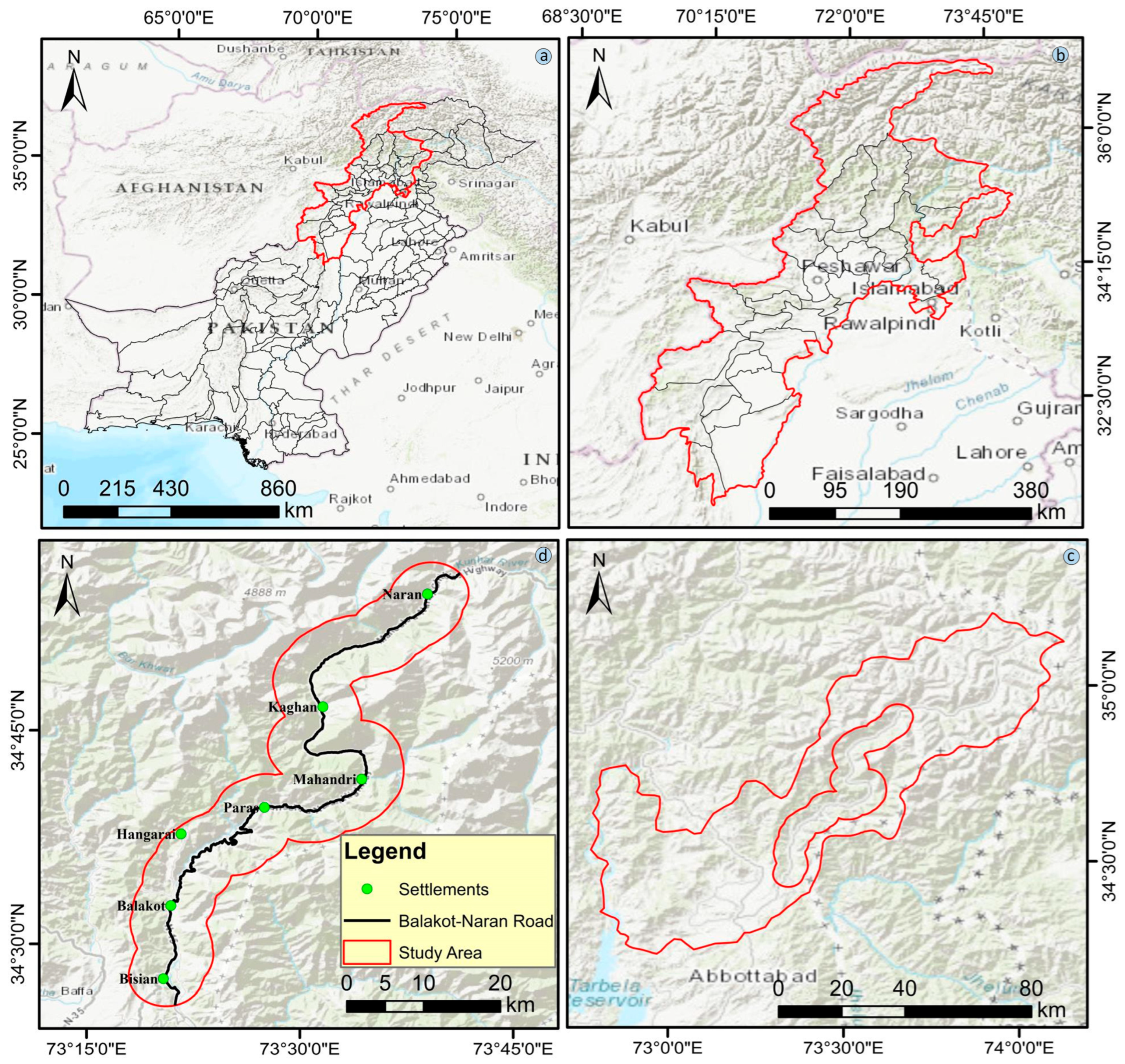
Figure 1. Geographical setting of the study area. (a) Pakistan, (b) province boundary, (c) district boundary, and (d) study area.
Remotesensing 17 03464 g001
Figure 2. Geographical technical route of study.
Remotesensing 17 03464 g002
Figure 3. Landslide inventory map of the study area (left). The inset panels (right) highlight representative landslide sites selected for detailed validation.
Remotesensing 17 03464 g003
Figure 4. LCFs. (a) Distance to road (m), (b) NDVI, (c) slope (°), (d) distance to faults (m), (e) geology: (1) Tanawal Formation and Manglaur Formations Undivided, (2) Sawat and Mansehra Granite Complexes Undivided, (3) Quaternary Alluvium, (4) Paleocene and Eocene Rocks Undivided, (5) Murree Formation, (6) Mesozoic Rocks Undivided, (7) Korara Complex and Gandaf Formations Undivided, (f) landcover: (1) urbanization, (2) water bodies, (3) subtropical Chir pine forest, (4) rangeland, (5) moist temperate coniferous forest, (6) alpine pasture, (7) snow, (8) dry temperate coniferous forest, (9) subalpine, (10) shrubs and bushes, (11) agriculture land, (g) distance to stream (m), (h) plan curvature, (i) profile curvature, (j) TWI, (k) curvature, (l) elevation (m), aspect, and (n) rainfall (mm).
Remotesensing 17 03464 g004
Figure 5. Interferograms generated using SBAS-InSAR with spatial–temporal baselines: (a) ascending track connection graph; (b) descending track connection graph.
Remotesensing 17 03464 g005
Figure 6. Feature importance obtained from the RFE technique.
Remotesensing 17 03464 g006
Figure 7. Mixed-association matrix for the fourteen landslide conditioning factors. Cells show absolute Spearman’s ρ (continuous–continuous), correlation ratio η (continuous–categorical), and Cramér’s V (categorical–categorical).
Remotesensing 17 03464 g007
Figure 8. Graphs of feature importance are shown in (a) bee swarm plots of SHAP values and (b) bar graphs of SHAP values.
Remotesensing 17 03464 g008
Figure 9. A dependency plot and a two-factor relationship plot of two factors: (a) a relationship between rainfall and slope, (b) a relationship between elevation and slope, and (c) a relationship between lithology and slope.
Remotesensing 17 03464 g009
Figure 10. LSM results. (a) AdaBoost model, (b) LightGBM model, (c) XGBoost model, and (d) hybrid model.
Remotesensing 17 03464 g010
Figure 11. An ROC curve is used to evaluate a model’s performance.
Remotesensing 17 03464 g011
Figure 12. Average evaluation metrics.
Remotesensing 17 03464 g012
Figure 16. Landslide-prone areas along the Balakot–Naran route identified using SBAS-InSAR.
Remotesensing 17 03464 g016
Table 1. List of LCFs used in the study.
S.NOVariablesSourcesResolutionDescription
1Slope, elevation, aspect, profile curvature, curvature, TWI, plan curvature, distance to streamsDigital elevation model 12.5 mALOS-PALSAR-DEM
(https://search.asf.alaska.edu/)
2Geology, distance to faults, distance to roadsGeological Map/Geological Survey of Pakistan
3LandcoverSentinel-2 imagery10 mLandcover
(https://earthexplorer.usgs.gov/)
4NDVISentinel-2 imagery10 mNormalized Different Vegetation Index
5RainfallGIOVANNI0.25°(https://giovanni.gsfc.nasa.gov/)
Table 2. Datasets used in SBAS-InSAR analysis.
DatasetsAscendingDescending
Product typeSentinel 1 SLC
PolarizationVV
Acquisition modeIW
No of images2424
Time periodJanuary 2022–December 2023
Frame112473
Track 100103
Table 3. RFE-derived quantitative feature importance and stability.
FeatureRF Weight (Normalized)RFE RankSelection Frequency
Slope0.17811
Aspect0.10411
Lithology0.10311
NDVI0.09911
Landcover0.09611
Elevation0.08611
Rainfall0.08611
Distance to Fault0.06711
Distance to Stream0.06211
Distance to Road0.05610.833
TWI0.04420.167
Plan Curvature0.01730
Profile Curvature0.00240
Curvature0.00150
Table 4. Assessment outcomes.
ModelAdaBoostLightGBMXGBoostHybrid
Full-14RFE-10Full-14RFE-10Full-14RFE-10Full-14RFE-10
AUC78.7279.5584.0084.3481.9284.8383.6688.00
Accuracy72.4073.7077.9279.5576.6276.3077.2780.52
Precision78.1778.3382.6584.1078.9782.5482.4784.69
Recall78.5781.1282.6583.6786.2279.5981.6384.70
F1 Score78.3779.6982.6583.1782.4481.0382.0584.69
MCC40.2542.4552.0055.8848.1049.5251.0957.90
MSE27.5926.1922.0020.4523.3723.7022.7319.48
RMSE52.5351.2847.0045.2248.3448.6847.6744.13
Disclaimer/Publisher’s Note: The statements, opinions and data contained in all publications are solely those of the individual author(s) and contributor(s) and not of MDPI and/or the editor(s). MDPI and/or the editor(s) disclaim responsibility for any injury to people or property resulting from any ideas, methods, instructions or products referred to in the content.