Abstract
Anomalous ionospheric disturbances have been observed as potential precursors to earthquakes. This study utilized data from the CSES satellite to investigate anomalies in the ULF band ionospheric electric field and electron density preceding earthquakes with magnitudes of Ms ≥ 6.0 in China and neighboring regions from 2019 to 2021. Comparative analysis with a randomly generated earthquake catalog indicated that these anomalies were spatially concentrated over the epicenter and temporally clustered on specific dates prior to the events. To assess the global relevance of these findings, the analysis was extended to earthquakes with Ms ≥ 7.0 worldwide during the same period, revealing consistent spatiotemporal patterns of ionospheric anomalies in both regional and global datasets. Furthermore, by combining the two earthquake catalogs and classifying events into oceanic and continental categories, additional statistical analyses were conducted to identify distinct ionospheric disturbance patterns associated with these different tectonic environments. These results provide a solid foundation for future research aimed at identifying and extracting ionospheric anomalies as potential pre-earthquake indicators.
1. Introduction
Earthquakes are among the most catastrophic natural disasters, often resulting in substantial human suffering, economic losses, and environmental destruction. Developing reliable methods for earthquake prediction has long been a central focus in geophysics and disaster mitigation research. Historical records of earthquakes span over four millennia, with some of the earliest documented accounts originating from China’s Xia Dynasty [1]. The invention of the seismoscope by Zhang Heng during the Han Dynasty marked a pioneering effort in systematic earthquake monitoring, and ancient texts and artifacts from various cultures provide evidence of observations of precursory phenomena [2]. The Industrial Revolution of the 19th century spurred significant advancements in science and technology, enabling more precise and comprehensive observations of earthquakes and their associated precursors [3,4,5,6]. Over time, the scope of exploration expanded from terrestrial and oceanic domains to the deep sea and outer space. By the mid-20th century, rapid progress in space technology heralded the “satellite era,” positioning the observation of Earth’s ionosphere, magnetosphere, and other outer atmospheric layers at the forefront of Earth science research [4].
Unlike weather forecasting, which has experienced considerable advancements driven by technological innovation, earthquake prediction remains a formidable challenge. The inaccessibility of the Earth’s interior has impeded progress, yet accumulating evidence indicates that ionospheric anomalies may serve as precursory signals for seismic events [7,8,9,10]. These anomalies present an innovative approach to identifying measurable pre-earthquake indicators, potentially representing a paradigm shift in the field of earthquake prediction.
Recent advancements in satellite technology and ionospheric research have unlocked new opportunities to investigate potential earthquake precursors in the Earth’s upper atmosphere [11,12,13]. A particularly promising area of study involves analyzing anomalous ionospheric disturbances, which have been observed to precede significant earthquakes in various regions across the globe [14,15,16]. Over the past two decades, research efforts have increasingly focused on characterizing the spatiotemporal properties of these disturbances and elucidating the physical mechanisms underlying their occurrence [8,17,18,19,20].
The ionosphere, a highly conductive region of Earth’s atmosphere characterized by elevated electron density, plays a crucial role in the propagation of electromagnetic waves. Perturbations in ionospheric parameters, including electric fields, ion density, and electron density, have been linked to seismic activity, suggesting their potential as pre-earthquake indicators [9,14,21,22,23,24,25,26]. Numerous studies have reported correlations between ionospheric anomalies and significant seismic events, revealing spatiotemporal patterns that imply a physical connection. For instance, Liu et al. [27,28,29] provided statistical evidence of Total Electron Content (TEC) anomalies preceding major earthquakes. Hayakawa et al. [30,31] and Pulinets and Ouzounov [32,33] proposed mechanisms linking lithospheric activity to ionospheric disturbances through electromagnetic and chemical coupling processes.
Beyond TEC and electric field variations, other ionospheric parameters have been examined for earthquake-related anomalies, including electron density profiles, geomagnetic variations, and plasma temperature. For example, Zhang et al. [34,35] analyzed ion density and plasma parameter changes prior to seismic events, while Sorokin et al. [17] and Stanica et al. [36] investigated geomagnetic variations and their relationships with impending earthquakes. The DEMETER satellite provided pioneering insights into the spatial and temporal characteristics of ionospheric disturbances associated with seismic activity [11,37,38,39], which were subsequently corroborated by missions such as Swarm and CSES [23,40,41,42,43,44]. These studies demonstrated how satellite data can distinguish seismic-related ionospheric anomalies from noise sources, such as solar flares, geomagnetic storms, or atmospheric phenomena [45,46,47,48].
Despite these advancements, significant challenges remain in understanding the variability and mechanisms of ionospheric anomalies. While some researchers support the Lithosphere–Atmosphere–Ionosphere Coupling (LAIC) model—suggesting that crustal stress accumulation generates electromagnetic emissions that alter ionospheric properties [8,18,44,49,50,51,52,53]—others propose alternative mechanisms, such as acoustic-gravity waves propagating upward from the Earth’s surface [54,55,56]. Meanwhile, skeptics argue that many observed anomalies may originate from non-seismic phenomena, such as space weather or artificial signals, rather than tectonic processes [57,58,59,60].
Regional studies have further highlighted variations in ionospheric anomalies based on tectonic settings. For instance, Yadav et al. [61] and Chakraborty et al. [62] observed differences in ionospheric responses between oceanic and continental earthquakes, while Riabova et al. [63] demonstrated the influence of local geomagnetic conditions on anomaly detection. Global datasets have offered additional insights, with numerous studies underscoring the importance of standardized methodologies to reduce noise and enhance reliability [64,65,66,67,68].
In this study, data from the China Seismo-Electromagnetic Satellite named “Zhangheng-1” satellite (hereinafter referred to as the CSES) were analyzed to investigate variations in ULF-band ionospheric electric fields and electron density preceding strong earthquakes. The analysis focuses on events with magnitudes of Ms ≥ 6.0 in China and neighboring regions from 2019 to 2021, as well as Ms ≥ 7.0 earthquakes globally during the same period. By comparing observed anomalies with a randomly generated earthquake catalog, this study aims to identify consistent spatiotemporal patterns and evaluate their potential as pre-earthquake indicators. Additionally, the study explores distinctions between oceanic and continental earthquakes to identify differences in ionospheric responses across tectonic environments.
The significance of this research lies in its contribution to the growing body of evidence supporting ionospheric disturbances as potential precursors to strong earthquakes. By leveraging satellite data and rigorous statistical methodologies, this study seeks to deepen the understanding of ionospheric behavior and its relationship to seismic activity, ultimately advancing efforts toward reliable earthquake prediction. The principal findings demonstrate the spatial and temporal clustering of ionospheric anomalies prior to earthquakes, as well as their applicability across diverse tectonic settings, thereby laying the groundwork for future research in this field.
2. Data
With advancements in satellite observation technology, humanity’s ability to investigate the upper atmosphere and ionosphere has improved significantly. A growing body of satellite-based research indicates that seismic activity can induce anomalous disturbances in various physical parameters of the ionosphere [60,61,69,70,71]. In recent years, China’s aerospace technology has made substantial progress, exemplified by the launch of the country’s first satellite dedicated to electromagnetic monitoring, the “CSES” satellite. Since its launch in 2018, the CSES has provided invaluable observational data for investigating the relationship between ionospheric precursor anomalies and earthquakes [9,23,43,44,72,73]. Operating at an orbital altitude of 507 km, the CSES offers extensive coverage and high-resolution observations, enabling detailed and comprehensive investigations of ionospheric disturbances [23,73].
The CSES delivers data of exceptional quality and resolution, offering crucial resources for exploring pre-seismic ionospheric anomalies (the data are published at https://leos.ac.cn (accessed on 23 May 2025) after registration). Researchers worldwide have utilized its data to analyze various ionospheric characteristics, contributing to the growing understanding of the link between ionospheric anomalies and seismic events [43,74,75]. Comparative studies with satellite observations from other nations and long-term data validation efforts have confirmed the reliability and accuracy of CSES data [76,77,78]. Nevertheless, research into ionospheric anomalies preceding earthquakes faces several challenges, particularly in terms of statistical sample sizes and regional applicability. Systematic statistical analyses using CSES data have the potential to uncover spatiotemporal correlations and patterns in pre-earthquake changes in ionospheric electric fields and electron density.
To further investigate the relationship between pre-seismic ionospheric disturbances and seismic events, this study employs ionospheric electric field data recorded by the electric field detector onboard the CSES, along with electron density data obtained from its Langmuir probe. The electric field data are categorized into four frequency bands based on their observation frequency: ultra-low frequency (ULF, DC–16 Hz), extremely low frequency (ELF, 6 Hz–2.2 kHz), very low frequency (VLF, 1.8 kHz–20 kHz), and high frequency (HF, 18 kHz–3.5 MHz) [43,76]. Numerous studies have demonstrated that ULF signals associated with pre-seismic ionospheric electric field anomalies can propagate to the ionosphere with minimal attenuation, inducing detectable disturbances [14,34,79]. As such, this study focuses specifically on ULF band electric field data for analysis.
The electric field detector onboard the CSES operates using an active double-probe measurement principle. It comprises four spherical sensors, four sensor cable assemblies, and a signal processing unit. To accurately capture the spatial distribution of three-dimensional electric fields, the detector deploys the four sensors outward from the satellite body using extendable booms, positioning each sensor 4.5 m away from the satellite. These sensors function as sensitive “antennas,” capable of detecting the ambient plasma environment’s potential. The electric field along the direction of two sensors is calculated as the ratio of the potential difference between the sensors to the distance separating them [76].
The Langmuir probe onboard the CSES, employed for measuring ionospheric electron density, represents one of the most widely adopted in situ space plasma diagnostic technologies globally and marks the first application of this technique on a Chinese satellite platform [47,80]. The Langmuir probe primarily measures in situ electron density and electron temperature in the ionosphere. Its operational principle involves inserting the probe (sensor) into the ionospheric plasma, where it collects electrons and ions to generate a current that reflects key ionospheric parameters such as electron density and temperature. When a scanning voltage is applied to the probe, the plasma current (I) collected varies with the applied bias voltage (Vb), forming an I-V characteristic curve that encapsulates the interaction between the probe and the surrounding plasma. By analyzing this I-V curve, parameters such as plasma density, electron temperature, floating potential, and plasma potential can be derived [81,82]. In this study, electron density data from the Langmuir probe is utilized for analysis.
The CSES orbits at an altitude of approximately 500 km, completing a full revolution around the Earth each day and following a revisit cycle of five days [83]. This means the satellite traverses the same orbital path every five days. Designed to support China’s earthquake prediction and early warning efforts, the satellite operates in two distinct modes: reconnaissance and detailed monitoring. The detailed monitoring mode is activated when the satellite passes over major seismic zones worldwide and regions within China, while the reconnaissance mode is used for other areas [83,84]. The monitoring frequency and precision enable researchers to use CSES data to observe ionospheric variations with high accuracy, facilitating the identification of pre-earthquake ionospheric anomalies.
It is important to acknowledge that the ionosphere, as the outermost layer of the Earth’s atmosphere, is a highly ionized region influenced by solar radiation and cosmic rays [85]. Due to its ionized and inherently unstable state, the ionosphere is particularly sensitive to space weather phenomena such as solar flares and geomagnetic storms [36,46,63]. Variations in solar activity directly affect ionization levels, increasing ion and free electron densities during periods of intense solar activity. Furthermore, fluctuations in solar activity influence electron density, with high-energy particle injections during active periods further amplifying ionospheric electron densities. Additionally, geomagnetic disturbances, caused by variations in the Earth’s magnetic field, can induce electromagnetic effects that alter ionospheric parameters, including electron density, altitude, and electric field intensity [75,86].
Given the ionosphere’s sensitivity to external influences, it is critical to account for solar and geomagnetic activity when analyzing ionospheric data. This study employs variations in the Ap index, Dst index, Kp index, and F10.7 index to quantify space environmental activity. The Ap index represents daily geomagnetic disturbance intensity, with values below 20 indicating geomagnetic quiet, 20–40 indicating minor disturbances, and values above 40 signifying severe disturbances [87]. The Dst index measures variations in the geomagnetic field caused by equatorial ring currents, with values below −30 nT indicating geomagnetic disturbances; lower values correspond to more intense disturbances. The Kp index reflects geomagnetic disturbance intensity, with values below 3 denoting quiet conditions, 4–6 representing minor-to-moderate storms, and 7–9 indicating major storms. The F10.7 index quantifies solar activity, with values exceeding 120 corresponding to high solar activity [84,88]. For this study, geomagnetic disturbances are defined as Ap > 20, Dst < −30 nT, or Kp > 3, while solar activity is considered intense when F10.7 > 120. Dates with any index exceeding these thresholds are classified as disturbed, and ionospheric data from these dates are excluded from analysis.
All earthquake catalog data used in this study were obtained from the China Earthquake Networks Center (CENC) (http://ceic.ac.cn (accessed on 23 May 2025)). Due to the skin effect of the Earth’s ionosphere, this study selected earthquakes with a hypocenter depth of less than 50 km.
3. Analysis Results
3.1. Analysis of Earthquake Cases: The 2021 Yangbi and Maduo Earthquakes in China
3.1.1. Analysis of Pre-Seismic Ionospheric Electron Density Anomalies
Given the substantial spatial variability of ionospheric parameters and the short time interval of only a few hours between the Yangbi and Maduo earthquakes, it was essential to account for and eliminate potential anomalies arising from spatial differences. Based on the geographic coordinates of the Yangbi and Maduo earthquake epicenters, the seismogenic zone of the larger-magnitude Maduo earthquake was designated as the reference. Data for this analysis were selected from all satellite tracks within 40° of longitude east and west of the Maduo epicenter, encompassing the range of 80°E–120°E.
Furthermore, since ionospheric electron density is significantly influenced by solar radiation, with daytime disturbances being far more pronounced than nighttime disturbances, this study utilized nighttime orbital data collected by the “CSES” satellite [23,73,89]. After filtering, it was determined that the satellite’s nighttime orbits over the Yangbi and Maduo epicenters occurred between 17:00 and 21:00 UTC, corresponding to 01:00–05:00 local time the following day, thereby satisfying the criteria for nighttime data collection.
The decision to use a 40° longitudinal range for the Yangbi and Maduo earthquake cases was primarily based on the following considerations:
1. Based on the empirical formula for the radius of the seismogenic zone proposed by Dobrovolsky et al. [90]:
The calculated radius for earthquakes with magnitudes of Ms ≥ 6.0 exceeds 380 km. Since seismic geological activities within the seismogenic zone may induce pre-seismic ionospheric anomalies, and one degree of longitude near 40°N corresponds to approximately 85 km, the seismogenic zone for Ms ≥ 6.0 earthquakes spans more than 5 degrees of longitude.
2. Ensuring that multiple satellite tracks pass over the epicenter daily allows for the collection of a more extensive dataset. This increased coverage helps reduce random errors and anomalies caused by the satellite itself, thereby improving the robustness of the analysis.
3. Previous studies on the Lithosphere–Atmosphere–Ionosphere Coupling (LAIC) mechanism suggest that spatial ionospheric effects generated during the earthquake preparation process may exhibit some displacement relative to the epicenter. Furthermore, anomalies can propagate horizontally within the same atmospheric layer, with a general spatial distribution ranging between 0° and 10° from the epicenter (Liu Jing et al., 2011) [91].
In summary, given that the Yangbi and Maduo earthquakes were analyzed as a single case due to their proximity and combined influence area, using a longitudinal range of ±40° from the epicenters is considered appropriate for this study. The relationship between the satellite track positions and the epicenters is illustrated in Figure 1.
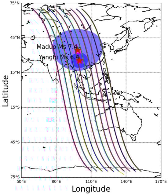
Figure 1.
Schematic diagram of all ascending orbital tracks of the CSES within ±40° longitude of the epicenters during the three months preceding the Yangbi and Maduo earthquakes. Each track is represented in a different color. The red pentagram indicates the epicenters of the mainshocks of the Yangbi and Maduo earthquakes. The dark purple solid circles and light purple solid circles represent the seismogenic zones of the Yangbi and Maduo earthquakes, respectively.
Following the definition of the study area, it is essential to minimize the influence of space weather activities on the analysis. To this end, variations in the Ap index, Dst index, Kp index, and F10.7 index are employed to characterize the overall activity of the space environment. Detailed descriptions of these indices are provided in Section 2.
Figure 2 illustrates the changes in space environment activity during the 30 days preceding the Yangbi and Maduo earthquakes. On 12–13 May, approximately ten days before the earthquakes, the Ap index exceeded 40, the Dst index dropped to −60, the Kp index approached 7, and the F10.7 index exhibited no significant changes. These observations indicate the occurrence of a major geomagnetic storm on 12 May, which subsided by May 13 as the space environment gradually returned to a stable state. This geomagnetic storm likely had a significant impact on the ionosphere.
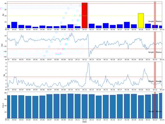
Figure 2.
The space environment activity information before the Yangbi and Maduo earthquakes is shown in the figure. From top to bottom, the subplots represent the Ap index, Dst index, Kp index, and F10.7 index, respectively. The red vertical lines indicate the occurrence times of the Yangbi and Maduo earthquakes, while the red dashed lines represent the upper and lower thresholds for geomagnetic quiet conditions.
Furthermore, on 20–21 May, one day before the earthquakes, the Ap index exceeded 20, the Dst index dropped to −30, the Kp index exceeded 5, and the F10.7 index again showed no notable changes. These conditions suggest the occurrence of a moderate geomagnetic storm on 20 May, which subsided by 21 May as the space environment stabilized. This geomagnetic storm likely also influenced ionospheric conditions.
Consequently, ionospheric data from 12 May and 20 May are excluded from this study to mitigate the impact of geomagnetic storms on the analysis.
The ionosphere is an inherently open and dynamic atmospheric layer where various disturbances occur daily across different regions, each exhibiting varying concentrations of ionized components. To accurately extract ionospheric anomalous disturbances, this study analyzes ionospheric electron density and electric field data collected by the “CSES” satellite for all ascending orbital tracks passing within ±40° longitude of the epicenters during the three months preceding the Yangbi and Maduo earthquakes. The analysis process for ionospheric electron density data is outlined as follows:
- Linear interpolation: For all ascending orbital tracks passing within ±40° longitude of the epicenters during the three months prior to the earthquakes, linear interpolation is performed at intervals of 0.1°latitude for each track. Similarly, the longitude data for each track are interpolated based on the longitudinal span of the track. This ensures that each interpolated ionospheric electron density value corresponds precisely to a specific latitude and longitude.
- Grouping by revisit tracks: All tracks are grouped into n sets based on their revisit cycles to enable consistent temporal analysis.
- Background field calculation: For each set of revisit tracks during the three months preceding the earthquakes, the median background field and interquartile range (IQR) of electron density are calculated to establish a reference for identifying anomalies. As shown in Figure 1, multiple revisit orbits pass over a specific satellite orbit of CSES. Therefore, in this study, all revisit orbit data along this orbit within three months before the earthquake were grouped together to calculate the median background field and anomalous perturbations. In addition, since the revisit cycle of the CSES is 5 days, using revisit orbits within three months before the earthquake to calculate the background field in this study ensures that more than ten orbits are included in the calculation, which helps maximize the reliability of anomalies.
- Anomaly percentage calculation: The percentage anomaly of the observed ionospheric electron density relative to the median background field is computed using the following formula:where represents the interpolated ionospheric electron density data, denotes the median background field of electron density, is set to 1.5 based on testing, and refers to the interquartile range. The thresholds for identifying anomalies are defined as .
- For the calculated , values exceeding 50% are defined as anomalies. However, since the satellite observations may be affected by operations such as instrument mode switching or flight attitude adjustments, which can cause abrupt jumps in data values and excessively large amplitude changes, an upper limit was determined after testing multiple thresholds. The final anomaly definition rule is as follows: values exceeding 50% but not exceeding 200% are considered anomalies.
After the above processing steps, the anomaly magnitude and percentage relative to the median background field can be obtained for each track. Figure 3 illustrates the raw ionospheric electron density data, the median background field, and the percentage relative variation in the background field and anomalies, using track 18203 as an example. The figure shows that large-scale anomalous disturbances occurred within more than 30° latitude above the Yangbi and Maduo epicenters, with disturbance magnitudes exceeding 50% of the median background field and even reaching up to 150%.
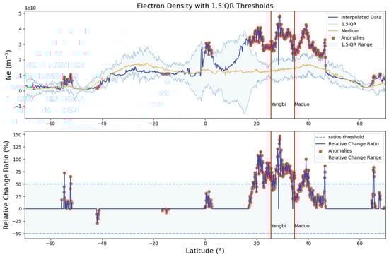
Figure 3.
Raw ionospheric electron density data, background field, and percentage variation relative to the background field for track 18203 at 03:00 on May 15. In the upper plot, the dark blue solid line represents the interpolated observation data, the yellow solid line represents the median background field, and the light blue solid line represents the background field. In the lower plot, the light blue dashed lines indicate the upper and lower thresholds for anomaly identification.
After applying the same method to calculate and plot the other global tracks recorded by the satellite on the same day, the results are shown in Figure 4. It is evident that significant ionospheric electron density anomalies were observed in track 18203 to the west of the epicenter. In contrast, the ionospheric electron density detected by other tracks of the CSES over Asia on the same day showed almost no variation after calculation.
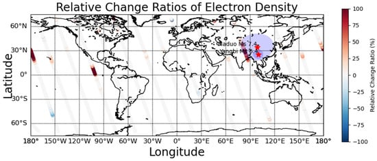
Figure 4.
Percentage Variation in Ionospheric Electron Density Anomalies Relative to the Background Field for All Global Tracks on May 15. Red five-pointed stars represent the epicenters of the Yangbi and Maduo earthquakes, while solid dark purple circles and solid light purple circles denote the ranges of the seismogenic zones of the Yangbi earthquake and Maduo earthquake, respectively.
Subsequently, using the same method, all tracks from one month prior to the earthquake were analyzed. It was found that 5 days before the earthquake (Figure 5 and Figure 6), track 18218; 4 days before the earthquake (Figure 7 and Figure 8), track 18233; and on the day of the earthquake (Figure 9), track 18294, all exhibited enhanced electron density disturbances within 20° above the epicenter. The disturbance amplitudes exceeded 50% and reached up to approximately 150%. Additionally, the spatial extent of each disturbance covered more than 5°in latitude and longitude (approximately 500 km). This indicates that the anomalies are unlikely to be related to instrumental noise and are highly likely associated with the earthquake.
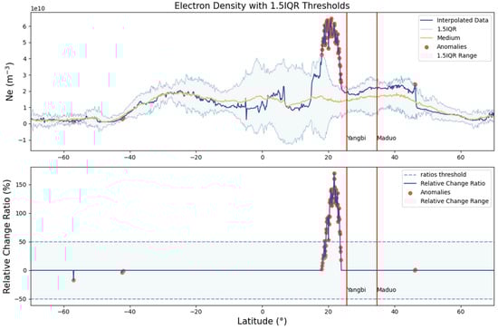
Figure 5.
Raw ionospheric electron density data, background field, and percentage variation relative to the background field for track 18218 at 03:00 on 16 May. In the upper plot, the dark blue solid line represents the interpolated observation data, the yellow solid line represents the median background field, and the light blue solid line represents the background field. In the lower plot, the light blue dashed lines indicate the upper and lower thresholds for anomaly identification.
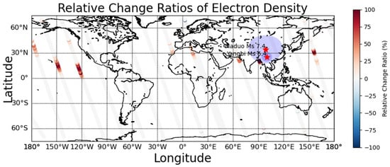
Figure 6.
Percentage Variation in Ionospheric Electron Density Anomalies Relative to the Background Field for All Global Tracks on 16 May. Red five-pointed stars represent the epicenters of the Yangbi and Maduo earthquakes, while solid dark purple circles and solid light purple circles denote the ranges of the seismogenic zones of the Yangbi earthquake and Maduo earthquake, respectively.
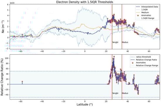
Figure 7.
Raw ionospheric electron density data, background field, and percentage variation relative to the background field for track 18233 at 03:00 on 17 May. In the upper plot, the dark blue solid line represents the interpolated observation data, the yellow solid line represents the median background field, and the light blue solid line represents the background field. In the lower plot, the light blue dashed lines indicate the upper and lower thresholds for anomaly identification.
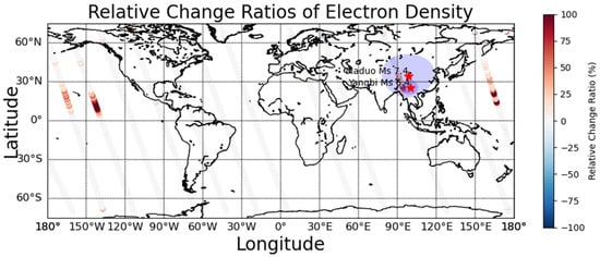
Figure 8.
Percentage Variation in Ionospheric Electron Density Anomalies Relative to the Background Field for All Global Tracks on 17 May. Red five-pointed stars represent the epicenters of the Yangbi and Maduo earthquakes, while solid dark purple circles and solid light purple circles denote the ranges of the seismogenic zones of the Yangbi earthquake and Maduo earthquake, respectively.
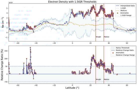
Figure 9.
Raw ionospheric electron density data, background field, and percentage variation relative to the background field for track 18294 at 03:00 on May 21. In the upper plot, the dark blue solid line represents the interpolated observation data, the yellow solid line represents the median background field, and the light blue solid line represents the background field. In the lower plot, the light blue dashed lines indicate the upper and lower thresholds for anomaly identification.
3.1.2. Analysis of Pre-Seismic Ionospheric Electric Field Anomalies
The electric field detector onboard the CSES is capable of recording both waveform data and power spectral density data of ionospheric electric fields. The stored electric field data are categorized into four frequency bands based on observation frequency: ULF, ELF, VLF, and HF bands. This study utilizes power spectral density data from the ULF band. Scientific studies have shown that electromagnetic signals exhibit fractal characteristics in some ground-based ultra-low-frequency magnetic field data processing [14,34,79].
According to the officially released scientific data file specification, the ULF electric field power spectral density data detected by the CSES primarily consist of three-component data in the DC–16 Hz range under detailed and survey observation modes. However, upon querying the stored data, it was found that the CSEScontains ULF electric field power spectral density data in the 0–21 Hz range. To conduct a detailed analysis of the electric field characteristics in different frequency ranges within the ULF band, this study divides the power spectral density (PSD) data into two frequency ranges, i.e., 0–10 Hz and 11–21 Hz, based on the results of preliminary calculations and comparative analyses. After organizing and analyzing the data, this study identified significant increases in the power spectral density of all three components of the electric field on 21 May for track 18293, particularly around 30°N latitude, as shown in Figure 10. Upon calculating the anomaly magnitude relative to the background field, Figure 11 reveals that the disturbance amplitude relative to the background field was substantial, exceeding ten times the upper limit of the anomaly percentage defined in this study. Additionally, the anomaly amplitudes in the X and Y components were greater than those in the Z component. This anomalous disturbance occurred at approximately 3:00 a.m. on the day of the mainshock, 18 h before the Yangbi earthquake, and falls within the pre-earthquake range. Such a large-scale anomaly was not reflected in our previous studies on atmospheric electric field anomalies before the Yangbi earthquake, warranting further investigation [92].
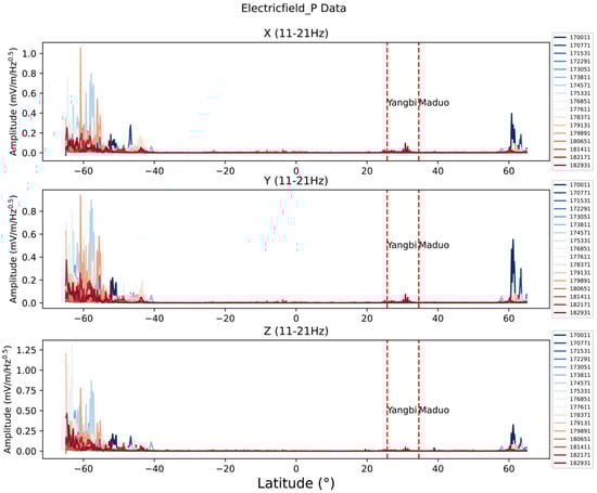
Figure 10.
The data variation process of the three components (11–21 Hz) of electric field power spectral density from the same set of revisiting orbits, spanning from three months before the earthquake to its occurrence. The upper, middle, and lower panels correspond to the electric field power spectral density data of the X, Y, and Z components, respectively. The red dashed lines denote the latitude of the main shock of the Yangbi and Maduo earthquakes.
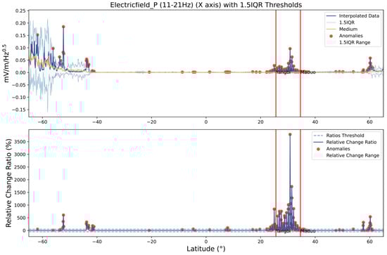
Figure 11.
Raw ionospheric electron density data, background field, and percentage variation relative to the background field for track 18294 at 03:00 on 21 May. In the upper plot, the dark blue solid line represents the interpolated observation data, the yellow solid line represents the median background field, and the light blue solid line represents the background field. In the lower plot, the light blue dashed lines indicate the upper and lower thresholds for anomaly identification.
3.2. Statistical Analysis of Ms ≥ 6.0 Earthquakes in China and Adjacent Regions from 2019 to 2021
Statistics reveal that over 90% of all earthquakes globally occur along the Pacific Ring of Fire and the Mediterranean–Himalayan seismic belt, collectively accounting for approximately 95% of the total seismic energy released worldwide [84,89]. Located between these two major seismic belts, China ranks among the most seismically active and intense regions on Earth. Historically, large earthquakes in mainland China have resulted in death tolls ranging from tens of thousands to hundreds of thousands, as well as substantial direct and indirect economic losses [93].
In this study, we investigated sixteen earthquake events with magnitudes of Ms ≥ 6.0 that occurred in China and adjacent areas between 2019 and 2021 (see Table 1 for details; their spatial distribution is illustrated in Figure 12). Due to their close temporal proximity, the Yangbi earthquake in Yunnan and the Maduo earthquake in Qinghai were combined and treated as a single event for analytical purposes. For each earthquake, median background fields of ionospheric electric fields and electron densities were constructed using observational data from the three months preceding the mainshock. Subsequently, anomalies in the power spectral density of ionospheric electric fields and electron densities within the month leading up to each mainshock were identified, following the anomaly detection methods described in the previous section.

Table 1.
Catalog of Ms ≥ 6.0 Earthquakes in China and Adjacent Regions from 2019 to 2021.
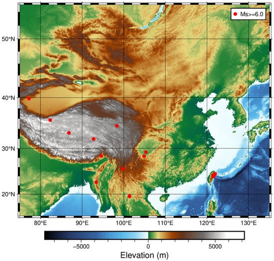
Figure 12.
Distribution of Ms ≥ 6.0 Earthquakes in China and Adjacent Regions from 2019 to 2021. Solid red dots indicate the locations of earthquake epicenters.
Following the identification of anomalies, the detection and extraction of pre-seismic disturbances may be confounded by non-seismic ionospheric anomalies in tropical regions, potentially induced by the equatorial ionization anomaly on both sides of the equator [94,95]. To address this challenge, the present study employs a random earthquake test method to verify the patterns and characteristics of pre-seismic anomalies observed in the earthquake catalog. The construction of the random earthquake catalog adheres to the following rules:
1. To investigate whether ionospheric electric field and electron density anomalies at the same epicenter during different periods are indeed related to earthquakes, the latitude, longitude, and depth of the original epicenter remain unchanged, and only the occurrence date is modified.
2. Each random earthquake occurs at least three months apart from its corresponding real earthquake, thereby minimizing the real event’s influence on the median background field of the random earthquake.
3. To minimize the impact of real earthquakes and their pre-earthquake perturbations on random earthquakes, each earthquake in the new catalog of random earthquakes is separated by at least one month in occurrence date from each earthquake in the catalog of real earthquakes.
4. Events in the random catalog are separated by at least one month. For earthquakes in the Sichuan–Yunnan region and those near Taiwan, this interval may be shorter but cannot be less than half a month.
Adhering to these guidelines, a random earthquake catalog was generated, as presented in Table 2. To evaluate differences in anomalies preceding real versus random earthquakes and to ascertain whether ionospheric disturbances are driven by seismic geological activity, the same procedures for constructing the median background field, calculating the interquartile range, and identifying and extracting anomalies were applied consistently to both sets of earthquakes.
Table 2.
Catalog of Ms ≥ 6.0 Earthquakes in China and Adjacent Regions (Random Earthquakes) from 2019 to 2021.
3.2.1. Ionospheric Electron Density Anomalies Before Ms ≥ 6.0 Earthquakes in China and Adjacent Regions from 2019 to 2021
For ionospheric electron density anomalies, this study processed and analyzed all electron density data from satellite tracks recorded within one month prior to each earthquake in the catalog, in accordance with the anomaly extraction rules established for individual earthquakes. The specific steps and rules are as follows:
1. Interpolation by Latitude
For every 0.1° latitude data point identified as anomalous, linear interpolation is performed at 1° latitude intervals. This procedure yields 141 data points between 70°S and 70°N for ionospheric electron density data and 131 data points between 65°S and 65°N for ionospheric electric field data.
2. Normalization of Geographic Coordinates
Each anomaly’s geographic coordinates are normalized by designating the earthquake epicenter as (0,0). The relative latitude is calculated as the anomaly’s latitude minus the epicenter’s latitude, producing a positive value if the anomaly is north of the epicenter and a negative value if it is south. Similarly, the relative longitude is determined by subtracting the epicenter’s longitude from the anomaly’s longitude, with a positive value indicating the anomaly is east of the epicenter and a negative value indicating it is west.
3. Magnitude Thresholds for Anomalies
The amplitude of each disturbance, measured against the median background field, must exceed +50% but remain below +200%, or fall below −50% but stay above −200%. This constraint preserves a reasonable disturbance range and minimizes the impact of non-seismic factors such as satellite mode switching or power cycling.
4. Point-Based Anomaly Validation
An anomaly point is discarded if it is not adjacent to another anomaly point (i.e., if neither the preceding nor following point is anomalous). Only anomaly points that border at least one other anomalous point are retained.
5. Track Quality Control
In some cases, the entire satellite track surpasses the defined anomaly thresholds, indicating potential data quality issues. If the number of anomaly points in a single track exceeds one-seventh of the total data points for that track—corresponding to anomalies spanning more than 20° of latitude—that track is deemed low-quality, and its anomalies are excluded from further analysis.
6. Selection of Closest Anomalies
If multiple anomalies of the same variable are detected on a single track, only the anomaly closest to the epicenter is recorded.
Utilizing these anomaly identification rules, we identified anomalies that may be associated with seismic activity during the earthquake preparation process. To visualize these anomalies, their relative latitudes and longitudes were plotted on a 2.5° × 2.5° grid, and the frequency of anomalies within each grid cell was recorded. The left subplot of Figure 13 displays the distribution of ionospheric electron density anomalies relative to their respective epicenters. Using the same procedure, anomalies for all random earthquakes in the random earthquake catalog were plotted separately, as illustrated in the right subplot of Figure 13.
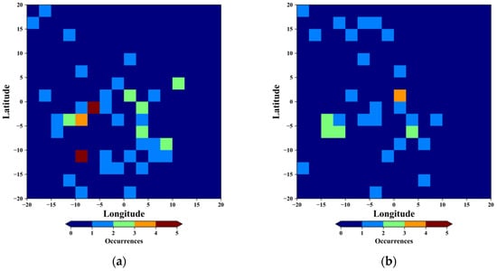
Figure 13.
Statistical Analysis of Electron Density Anomalies Relative to Epicentral Latitude and Longitude Before Ms ≥ 6.0 Earthquakes (a) and Random Earthquakes (b) in China and Adjacent Regions from 2019 to 2021.
Results from the earthquake catalog indicate that pre-seismic electron density anomalies predominantly occur south of the epicenter, with notable concentrations to both the west and east. The eastern and southeastern sectors exhibit broader anomaly ranges, whereas the western sector presents a more localized distribution, with more than three anomalies appearing in three distinct grid cells. These observations are consistent with prior research findings.
When comparing the earthquake catalog to the random earthquake catalog, the frequency of pre-seismic ionospheric electron density anomalies is considerably higher in the former. By contrast, anomalies in the random catalog remain sparse; only one grid cell, located slightly east of the epicenter, contains three anomalies, which are likely attributable to post-seismic ionospheric disturbances.
Furthermore, anomalies directly overhead the epicenter seldom occur in the earthquake catalog, a result that aligns with earlier studies indicating that pre-seismic ionospheric electrons tend to migrate horizontally. Consequently, the ensuing anomalies often appear within a latitudinal and longitudinal range of roughly 10° from the epicenter [91,96,97].
After examining the spatial distribution of ionospheric electron density anomalies, we next calculated the time interval between each pre-seismic anomaly and its corresponding mainshock. As discussed in the previous section, we obtained the relative latitudes and longitudes of anomalies with respect to each epicenter. By applying these relative coordinates, we determined the distance between each anomaly and the corresponding mainshock epicenter. In this study, distances between two geographic coordinates were computed using the Haversine formula [98]:
where r is the mean Earth radius (6371 km), lon1 and lat1 represent the longitude and latitude of the mainshock epicenter, and lon2 and lat2 represent the longitude and latitude of the anomaly location, respectively.
Figure 14 (left panel) presents the statistical results of ionospheric electron density anomalies in terms of their timing relative to the mainshock and their distance from the epicenter. Applying the same analytical procedure, we plotted the anomalies detected in the random earthquake catalog separately, as shown in Figure 14 (right panel).
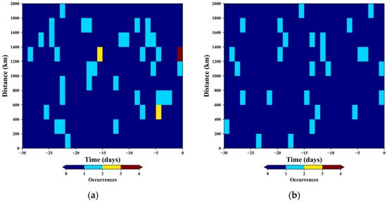
Figure 14.
Statistical Results of the Spatiotemporal Relationship of Electron Density Anomalies Before Ms ≥ 6.0 Earthquakes (a) and Random Earthquakes (b) in China and Adjacent Regions from 2019 to 2021. The horizontal axis represents the time of anomaly occurrence, and the vertical axis represents the distance between the anomaly and the epicenter.
From these data, it is evident that pre-seismic ionospheric electron density anomalies exhibit periodic fluctuation patterns. Specifically, anomalies occurred frequently approximately 20–25 days before the mainshock, after which the ionosphere remains relatively calm. Around 15 days prior to the earthquake, anomalies reappeared, followed by another decrease. Subsequently, beginning about 5 days before the mainshock, anomalies intensified again until the earthquake occurred. Additionally, the distance of these anomalies from the epicenter follows a discernible trend: about 25 days before the earthquake, anomalies appear both near the epicenter and at distances exceeding 1000 km. Around 15 days prior to the earthquake, anomalies are observed only at distances greater than 1000 km, suggesting that they temporarily migrate farther away from the epicenter. However, starting from around 10 days before the earthquake, these anomalies progressively shift closer to the epicenter as the mainshock approaches.
When the statistical outcomes of real earthquakes and random earthquakes are compared, the random earthquake catalog does exhibit some potential anomalies; however, they occur more irregularly. In contrast, pre-seismic electron density anomalies in real earthquakes are more concentrated in the periods 15–20 days and 5–10 days before the earthquake, a pattern closely resembling that observed in the previously noted atmospheric electric field anomalies preceding earthquakes [92].
3.2.2. Ionospheric Electric Field Power Spectral Density Anomalies Before Ms ≥ 6.0 Earthquakes in China and Adjacent Regions from 2019 to 2021
In the preceding section, we examined the ionospheric electron density anomalies and electric field power spectral density anomalies that occurred prior to the Yangbi earthquake. Building on this analysis, the present study performed a statistical assessment of pre-seismic ionospheric electric field power spectral density anomalies using both the main earthquake catalog and the random earthquake catalog.
Specifically, six datasets were derived from power spectral density measurements in the X, Y, and Z components, within two frequency ranges: 0–10 Hz and 11–21 Hz. These datasets were subjected to the same analytic procedures as the electron density data. Figure 15 presents the anomaly occurrence frequencies relative to the latitudinal and longitudinal positions of the respective epicenters. Subplots a, b, and c depict the occurrence frequencies of anomalies in the 0–10 Hz band for the X, Y, and Z components, whereas subplots d, e, and f illustrate the corresponding results for the 11–21 Hz band.
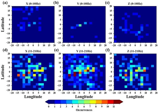
Figure 15.
Statistical Analysis of Electric Field Power Spectral Density Anomalies Relative to Epicentral Latitude and Longitude Before Ms ≥ 6.0 Earthquakes in China and Adjacent Regions from 2019 to 2021. (a), (b), and (c) correspond to the X, Y, and Z components in the 0–10 Hz frequency band, respectively; (d), (e), and (f) correspond to the X, Y, and Z components in the 11–21 Hz frequency band, respectively.
These figures indicate that the electric field power spectral density anomalies before earthquakes exhibit a higher frequency of occurrence compared with electron density anomalies. A comparison across the two frequency bands reveals that anomalies are substantially more prevalent in the 11–21 Hz range, while almost no anomalies are observed in the 0–10 Hz range. In the 11–21 Hz band, anomalies for all three components (X, Y, and Z) cluster around the epicenter, extending significantly in the west–east direction. Notably, the Z component shows a marked concentration of anomalies south of the epicenter. This pronounced horizontal (east–west) distribution of power spectral density anomalies is reminiscent of the characteristics identified in the electron density anomalies.
Furthermore, in the 0–10 Hz band, the X and Y components display some anomalies near the epicenter, with distributions again stretching west–east. Interestingly, anomalies in the Z component at 0–10 Hz exhibit a ring-shaped pattern centered on the epicenter, with a radius of approximately 10°. Further research is warranted to elucidate the underlying cause of this distinctive feature.
For the statistical analysis of electric field power spectral density (PSD) anomalies relative to the number of days prior to an earthquake and their distances from the epicenter, the results are presented in Figure 16. Overall, anomalies in the X, Y, and Z components occur more frequently in the 11–21 Hz frequency band, whereas they are relatively uncommon in the 0–10 Hz band.
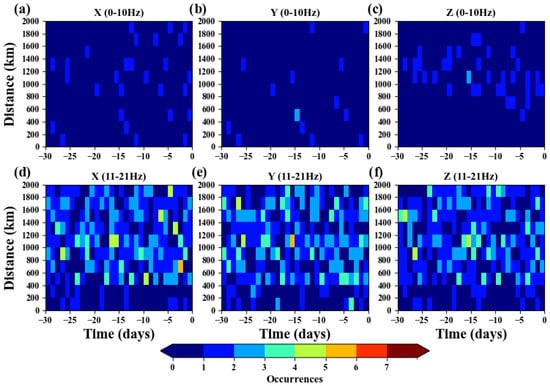
Figure 16.
Statistical Results of the Spatiotemporal Relationship of Electric Field Power Spectral Density Anomalies Before Ms ≥ 6.0 Earthquakes in China and Adjacent Regions from 2019 to 2021. The horizontal axis represents the time of anomaly occurrence, and the vertical axis represents the distance between the anomaly and the epicenter. (a), (b), and (c) correspond to the X, Y, and Z components in the 0–10 Hz frequency band, respectively; (d), (e), and (f) correspond to the X, Y, and Z components in the 11–21 Hz frequency band, respectively.
In the 0–10 Hz band specifically, the X and Y components share similar anomaly patterns, exhibiting concentrated occurrences around 25–30 days, 10–15 days, and 5 days before the earthquake. By contrast, the Z component displays a different pattern, with anomalies appearing closer to the epicenter as the mainshock approaches; moreover, the frequency of Z-component anomalies increases as the event date nears.
In the 11–21 Hz band, anomalies in the PSD of all three components appear most frequently approximately 25 days, 15 days, and 5 days before the earthquake, particularly at distances of 400–1200 km from the epicenter. Within 400 km of the epicenter, anomalies are almost absent. In addition, between 15 and 5 days before the earthquake, a decrease in anomaly occurrence is observed for all three components. This pattern is consistent with the atmospheric electric field anomalies recorded at multiple stations prior to the Yangbi earthquake, as described in previous sections.
Furthermore, electric field PSD anomalies concentrate at around 1000 km from the epicenter. Near 30°N latitude, one degree of longitude corresponds to roughly 96 km, implying that these anomalies span about 10° of longitude. This finding aligns with prior research indicating horizontal migration of ionospheric anomalies and corroborates the ionospheric electric field and electron density anomaly characteristics identified earlier in this study [99,100].
To assess the generalizability and enhance the reliability of the pre-seismic electric field power spectral density anomalies identified in the primary earthquake catalog, the same methodology was applied to the random earthquake catalog. Figure 17 shows the statistical results for the frequency of anomalies relative to each epicenter’s latitude and longitude.
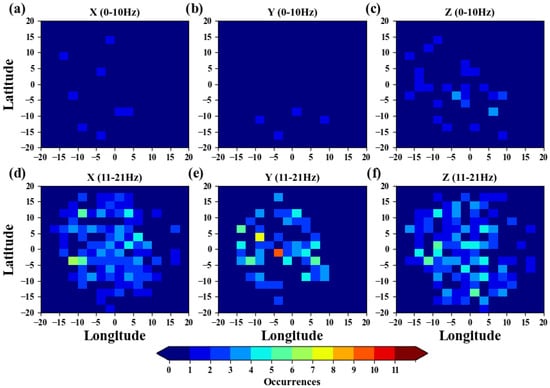
Figure 17.
Statistical Analysis of Electric Field Power Spectral Density Anomalies Relative to Epicentral Latitude and Longitude Before Ms ≥ 6.0 Random Earthquakes in China and Adjacent Regions from 2019 to 2021. (a), (b), and (c) correspond to the X, Y, and Z components in the 0–10 Hz frequency band, respectively; (d), (e), and (f) correspond to the X, Y, and Z components in the 11–21 Hz frequency band, respectively.
As illustrated in the figure, anomalies in the 0–10 Hz frequency band occur considerably less frequently compared with those in the 11–21 Hz band. Overall, for the random earthquake catalog, the electric field power spectral density anomalies in all three components appear far less often than their counterparts in the actual earthquake catalog; in most grid cells, the number of anomalies does not exceed four. An exception arises in the 11–21 Hz band for the Y component, which exhibits nine anomalies within a grid cell west of the epicenter, directly overhead. These anomalies may stem from disturbances related to seismic activity. Nonetheless, it is also possible that the observed anomalies in the random earthquake catalog reflect ionospheric disturbance signals associated with post-seismic effects.
Next, the study conducted a statistical assessment of electric field power spectral density anomalies preceding random earthquakes, focusing on the number of days before the event and the distance from the epicenter (see Figure 18). Compared with real earthquakes, the overall occurrence frequency of electric field power spectral density anomalies in the random earthquake catalog is markedly lower, regardless of the frequency band (0–10 Hz or 11–21 Hz) or the component (X, Y, or Z). Moreover, no clear pattern emerges for these anomalies in the random catalog.
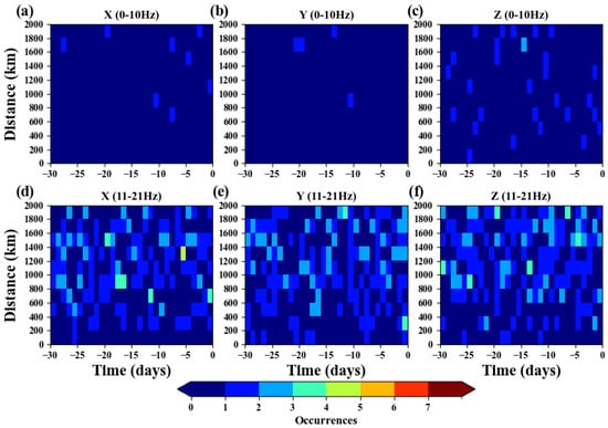
Figure 18.
Statistical Results of the Spatiotemporal Relationship of Electric Field Power Spectral Density Anomalies Before Ms ≥ 6.0 Random Earthquakes in China and Adjacent Regions from 2019 to 2021. The horizontal axis represents the time of anomaly occurrence, and the vertical axis represents the distance between the anomaly and the epicenter. (a), (b), and (c) correspond to the X, Y, and Z components in the 0–10 Hz frequency band, respectively; (d), (e), and (f) correspond to the X, Y, and Z components in the 11–21 Hz frequency band, respectively.
Notably, in the 11–21 Hz band—where anomalies are generally more frequent—almost no anomalies are observed within 1200 km of the epicenter. Instead, they tend to occur at distances exceeding 1400 km. These findings further corroborate the objective presence of pre-seismic electric field power spectral density anomalies.
3.3. Statistical Analysis of Ms ≥ 7.0 Earthquakes Worldwide from 2019 to 2021
In the previous section, this study conducted a statistical assessment of the spatiotemporal distribution of ionospheric electric field and electron density anomalies before earthquakes in China and adjacent regions. To determine whether these findings are globally applicable, we selected 19 earthquakes with magnitudes of Ms ≥ 7.0 that occurred worldwide between 2019 and 2021 (see Table 3), with their distribution shown in Figure 19.
Table 3.
Catalog of Ms ≥ 7.0 Earthquakes Worldwide from 2019 to 2021.
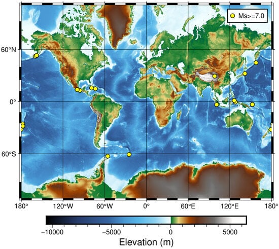
Figure 19.
Distribution of Ms ≥ 7.0 Earthquakes Worldwide from 2019 to 2021. Solid yellow dots indicate the locations of earthquake epicenters.
Because these earthquakes are numerous and dispersed globally, the distances between adjacent events are substantially larger, thereby minimizing mutual interference. Consequently, the time interval between two successive events can be less than one month. Furthermore, taking the skin effect into consideration, we focused only on earthquakes with focal depths shallower than 50 km. Furthermore, earthquakes with a time interval of less than one day are treated as a single earthquake in this study. This selection process ensures that the global earthquake catalog employed in this study remains highly reliable.
To compare the pre-seismic anomaly patterns identified in China and adjacent regions with those on a global scale—and to ascertain whether the ionospheric electric field and electron density anomalies detected in this study have universal applicability—the same analytical and statistical methods used for the Chinese and adjacent region catalog were applied to the global earthquake catalog. The left panel of Figure 20 shows the statistical results of anomaly occurrence frequency relative to each epicenter’s latitude and longitude, while the right panel of Figure 20 depicts the statistical results of anomaly occurrence frequency relative to the number of days before the earthquake and the distance from the epicenter.
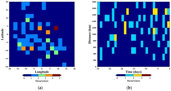
Figure 20.
Statistical Analysis of Electron Density Anomalies Relative to Epicentral Latitude and Longitude Before Ms ≥ 7.0 Earthquakes Worldwide from 2019 to 2021 (a) and Spatiotemporal Relationship of Anomalies (b). In the right panel, the horizontal axis represents the time of anomaly occurrence, and the vertical axis represents the distance between the anomaly and the epicenter.
The distribution of electron density anomalies in the left panel of Figure 20 closely resembles that observed in China and adjacent regions. Anomalies predominantly occur near the epicenter, exhibiting a marked east–west orientation, with multiple grid points in the east–west direction showing concentrated anomalies. Moreover, anomalies appear more frequently south of the epicenter. The right panel of Figure 20 presents the frequency of electron density anomalies in relation to the number of days prior to the mainshock and their distance from the epicenter. Evidently, pre-seismic electron density anomalies mainly occur within 400–1800 km of the epicenter, recurring approximately 25 days, 15 days, 5 days, and within 1 day before the earthquake. Furthermore, these anomalies shift closer to the epicenter as the mainshock approaches.
Overall, these patterns in the global earthquake catalog closely align with those derived from the Chinese and adjacent region catalog. In addition, because the global catalog features more earthquakes of higher magnitudes, the electron density anomaly frequency is greater, and the anomaly distribution patterns are more pronounced.
Regarding electric field power spectral density (PSD) observations, the same processing and analytical methods applied to the earthquake catalog for China and adjacent regions were utilized for global Ms ≥ 7.0 earthquakes from 2019 to 2021. Figure 21 displays the statistical results of anomaly occurrence frequency with respect to the epicenter’s latitude and longitude. Subplots a, b, and c illustrate the X, Y, and Z components in the 0–10 Hz frequency band, whereas subplots d, e, and f present corresponding results for the 11–21 Hz band.
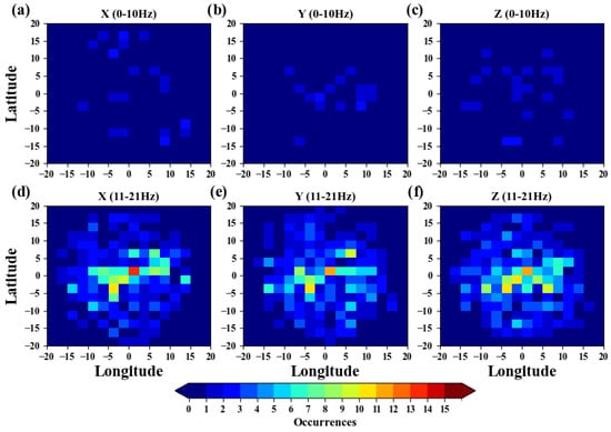
Figure 21.
Statistical Analysis of Electric Field Power Spectral Density Anomalies Relative to Epicentral Latitude and Longitude Before Ms ≥ 7.0 Earthquakes Worldwide from 2019 to 2021. (a), (b), and (c) correspond to the X, Y, and Z components in the 0–10 Hz frequency band, respectively; (d), (e), and (f) correspond to the X, Y, and Z components in the 11–21 Hz frequency band, respectively.
A comparison of these subplots reveals that anomalies are more prevalent in the 11–21 Hz range and cluster within a circular zone extending roughly 15° in both latitude and longitude around the epicenter. Beyond this boundary—approximately 20° northwest or southeast of the epicenter—anomalies are virtually absent. Relative to the pre-seismic PSD anomalies identified in the Chinese and adjacent region catalog, the global earthquake catalog demonstrates a higher frequency and a more pronounced concentration of anomalies prior to earthquakes. Notably, in the 11–21 Hz band, the grid cell located slightly east of the epicenter exhibits the highest anomaly occurrence, with 13 anomalies in the X component and 11 in both the Y and Z components. This finding implies that over 50% of global Ms ≥ 7.0 earthquakes are associated with such PSD anomalies.
Consistent with the anomaly distribution characteristics observed in the Chinese and adjacent region catalog, the 11–21 Hz anomalies in the X, Y, and Z components for global earthquakes also concentrate near the epicenter and display a predominantly east–west orientation. This trend, which is even more pronounced in the global dataset—where oceanic earthquakes constitute a substantial fraction—provides strong evidence supporting the notion that these anomalies involve horizontal migration within the ionosphere.
Furthermore, in the 0–10 Hz band, Z-component anomalies (see subplot c) exhibit a ring-shaped distribution, mirroring the results from the Chinese and adjacent region earthquake catalog. However, this phenomenon does not appear in the X and Y components at the same frequency. A possible explanation is that electric fields in the Z direction are more likely to penetrate the Earth’s atmosphere and propagate to ionospheric altitudes, thereby generating vertical atmospheric electric field anomalies and corresponding Z-component PSD anomalies within the ionosphere.
Additionally, a statistical analysis was conducted to investigate the relationship between electric field power spectral density (PSD) anomalies and both their temporal proximity to the earthquake and their distance from the epicenter in global Ms ≥ 7.0 earthquakes (Figure 22). Overall, the anomalies in the 11–21 Hz frequency band for the X, Y, and Z components occurred more frequently and exhibited clearer distribution patterns.
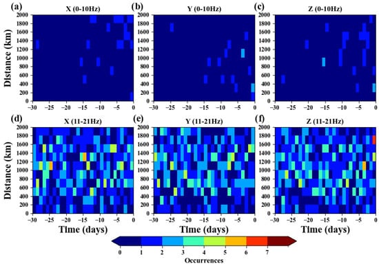
Figure 22.
Statistical Results of the Spatiotemporal Relationship of Electric Field Power Spectral Density Anomalies Before Ms ≥ 7.0 Earthquakes Worldwide from 2019 to 2021. The horizontal axis represents the time of anomaly occurrence, and the vertical axis represents the distance between the anomaly and the epicenter. (a), (b), and (c) correspond to the X, Y, and Z components in the 0–10 Hz frequency band, respectively; (d), (e), and (f) correspond to the X, Y, and Z components in the 11–21 Hz frequency band, respectively.
Within the 11–21 Hz range, anomalies were predominantly observed 25–30 days, 10–15 days, and 5 days before the earthquake, clustering at distances of 400–1600 km from the epicenter. Compared with the PSD anomalies identified prior to earthquakes in China and adjacent regions, the 0–10 Hz band for global events showed almost no anomalies between 15 and 30 days before the earthquake. Instead, anomalies began to appear only about 15 days prior to the mainshock, subsequently migrating closer to the epicenter as the earthquake approached. This difference may suggest that distinct earthquake types produce different patterns of pre-seismic anomalies.
Furthermore, ionospheric electric field anomalies were detected more frequently within 400 km of the epicenter for global earthquakes, reflecting the trend that higher-magnitude events are associated with more frequent and pronounced anomalies.
3.4. Statistical Analysis of Pre-Seismic Ionospheric Electric Field and Electron Density for Oceanic and Continental Earthquakes
Oceanic and continental earthquakes represent two distinct categories of seismic events. Their disparate environmental settings, geological structures, and other characteristics often give rise to variations in pre-seismic anomalies. To examine potential similarities and differences in precursor anomalies for these two earthquake types, this study reorganized the earthquake catalog after analyzing global Ms ≥ 7.0 earthquakes and Ms ≥ 6.0 earthquakes in China and adjacent regions. Based on each event’s geographic location, the global and regional earthquake catalogs discussed in the previous section were divided into oceanic and continental subsets. The ionospheric electric field power spectral density (PSD) anomalies and ionospheric electron density anomalies occurring within one month prior to each event were then analyzed according to these classifications.
Focusing first on ionospheric electron density anomalies, Figure 23 presents the statistical results of anomaly occurrence frequency relative to the epicenter’s latitude and longitude for oceanic earthquakes (left) and continental earthquakes (right) that occurred between 2019 and 2021. Comparing these two plots clearly demonstrates that ionospheric electron density anomalies appeared more frequently before oceanic earthquakes. Additionally, anomalies in both oceanic and continental events were concentrated southwest and east of the epicenter, with fewer anomalies observed to the north. Moreover, the anomalies extended horizontally in an east–west direction, consistent with the spatial distribution patterns identified for global and regional earthquakes in the preceding section.
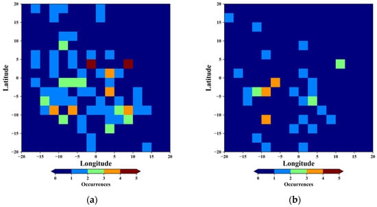
Figure 23.
Statistical Analysis of Electron Density Anomalies Relative to Epicentral Latitude and Longitude Before Global Oceanic Earthquakes (a) and Continental Earthquakes (b) from 2019 to 2021.
A statistical analysis was performed to examine electron density anomaly occurrence in relation to both the number of days before an earthquake and the distance from the epicenter for global oceanic and continental earthquakes occurring from 2019 to 2021. The results are displayed in Figure 24, with the left panel corresponding to oceanic earthquakes and the right panel to continental earthquakes.
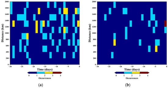
Figure 24.
Statistical Results of the Spatiotemporal Relationship of Electron Density Anomalies Before Global Oceanic Earthquakes (a) and Continental Earthquakes (b) from 2019 to 2021. The horizontal axis represents the time of anomaly occurrence, and the vertical axis represents the distance between the anomaly and the epicenter.
The findings suggest that, in comparison with continental earthquakes, anomalies appear more frequently prior to oceanic earthquakes. Nonetheless, for both oceanic and continental events, the anomalies concentrate primarily within 800–1600 km of the epicenter.
Regarding the temporal distribution of anomalies, both oceanic and continental earthquakes exhibit elevated anomaly frequencies approximately 20–25 days and 5 days before the event. The key difference arises around 15 days prior to the earthquake: oceanic earthquakes display a higher frequency of anomalies during this interval, whereas continental earthquakes show fewer anomalies. This pattern partially deviates from the conclusions drawn in the previous section, potentially due to the relatively lower magnitudes of earthquakes in the continental earthquake catalog.
The statistical analysis of ionospheric electron density anomalies preceding oceanic and continental earthquakes revealed distinct differences. To further investigate these variations, this study analyzed pre-seismic ionospheric electric field PSD anomalies for oceanic and continental earthquakes. Figure 25 and Figure 26 display the statistical results of PSD anomaly occurrence frequencies relative to the epicenters’ latitude and longitude for global oceanic and continental earthquakes occurring between 2019 and 2021. Figure 25 presents the results for oceanic earthquakes, while Figure 26 shows the results for continental earthquakes.
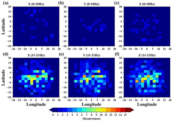
Figure 25.
Statistical Analysis of Electric Field Power Spectral Density Anomalies Relative to Epicentral Latitude and Longitude Before Global Oceanic Earthquakes from 2019 to 2021. (a), (b), and (c) correspond to the X, Y, and Z components in the 0–10 Hz frequency band, respectively; (d), (e), and (f) correspond to the X, Y, and Z components in the 11–21 Hz frequency band, respectively.
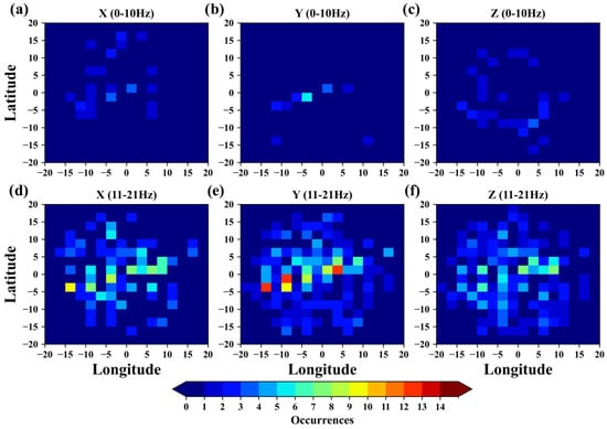
Figure 26.
Statistical Analysis of Electric Field Power Spectral Density Anomalies Relative to Epicentral Latitude and Longitude Before Global Continental Earthquakes from 2019 to 2021. (a), (b), and (c) correspond to the X, Y, and Z components in the 0–10 Hz frequency band, respectively; (d), (e), and (f) correspond to the X, Y, and Z components in the 11–21 Hz frequency band, respectively.
From these figures, it is apparent that for both oceanic and continental earthquakes, the occurrence frequency of PSD anomalies in the 0–10 Hz frequency band is significantly lower than that in the 11–21 Hz band. In the 11–21 Hz band, anomalies for both earthquake types exhibit a distinct east–west directional distribution centered above the epicenter. However, notable differences in the distribution patterns between oceanic and continental earthquakes are observed. Oceanic earthquakes show a higher overall frequency of PSD anomalies in the 11–21 Hz band, with anomalies particularly concentrated in the grid cell directly above the epicenter. By contrast, for continental earthquakes, anomalies are primarily observed at a distance of approximately 5° longitude from the epicenter, with no anomalies detected directly above the epicenter.
In the 0–10 Hz frequency band, both oceanic and continental earthquakes display ring-shaped anomaly distribution patterns with a radius of approximately 10° in latitude and longitude for the X and Z components. This phenomenon is consistent with the findings from the previous analysis of the global earthquake catalog.
To investigate pre-seismic electric field power spectral density (PSD) anomalies, this study conducted a statistical analysis of anomaly occurrence frequency relative to the number of days before the earthquake and their distances from the epicenter for global oceanic and continental earthquakes from 2019 to 2021. The results are presented in Figure 27 and Figure 28, with Figure 27 corresponding to oceanic earthquakes and Figure 28 to continental earthquakes.
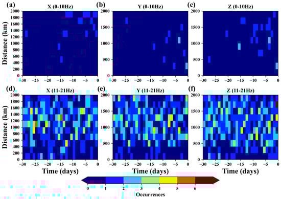
Figure 27.
Statistical Results of the Spatiotemporal Relationship of Electric Field Power Spectral Density Anomalies Before Ms ≥ 7.0 Global Oceanic Earthquakes from 2019 to 2021. The horizontal axis represents the time of anomaly occurrence, and the vertical axis represents the distance between the anomaly and the epicenter. (a), (b), and (c) correspond to the X, Y, and Z components in the 0–10 Hz frequency band, respectively; (d), (e), and (f) correspond to the X, Y, and Z components in the 11–21 Hz frequency band, respectively.
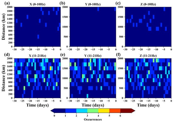
Figure 28.
Statistical Results of the Spatiotemporal Relationship of Electric Field Power Spectral Density Anomalies Before Ms ≥ 7.0 Global Continental Earthquakes from 2019 to 2021. The horizontal axis represents the time of anomaly occurrence, and the vertical axis represents the distance between the anomaly and the epicenter. (a), (b), and (c) correspond to the X, Y, and Z components in the 0–10 Hz frequency band, respectively; (d), (e), and (f) correspond to the X, Y, and Z components in the 11–21 Hz frequency band, respectively.
The analysis reveals that anomalies in the 11–21 Hz frequency band occur significantly more frequently than those in the 0–10 Hz band for both oceanic and continental earthquakes. Additionally, the total number of pre-seismic anomalies observed before oceanic earthquakes is higher than that before continental earthquakes. In the 11–21 Hz band, anomalies preceding oceanic earthquakes are predominantly concentrated within a range of 600–1600 km from the epicenter, whereas anomalies preceding continental earthquakes tend to occur more frequently beyond 1000 km from the epicenter.
In terms of temporal distribution, PSD anomalies for oceanic earthquakes exhibit a more pronounced pattern, with anomalies primarily occurring approximately 25 days, 15 days, and within 5 days before the mainshock. In contrast, anomalies before continental earthquakes are less clearly concentrated. Among the components, only the X component shows a higher frequency of anomalies around 15 days and 5 days before the earthquake, predominantly at distances of approximately 1000 km and 1500 km from the epicenter. This discrepancy may be attributed to the relatively smaller magnitudes of the continental earthquakes analyzed in this study.
Furthermore, in the 0–10 Hz frequency band, pre-seismic anomalies begin to appear approximately 15 days prior to oceanic earthquakes. For continental earthquakes, anomalies are observed in the X and Z components within 30 days before the mainshock, whereas no anomalies are detected in the Y component during the same period.
4. Discussion
Earthquakes occur deep underground and, unlike weather phenomena, are neither visible nor directly tangible [4]. As a result, despite the relatively advanced state of Earth observation technology and the increasing availability of observational data, earthquake prediction remains a formidable global challenge. Early studies have identified certain correlations between seismic activity and pre-seismic ionospheric anomalies [9,101,102,103]. However, not all earthquakes are preceded by such anomalies, and the characteristics of these anomalies, when they do occur, can vary significantly [104,105]. Although substantial progress has been made in the international research on pre-seismic ionospheric anomalies—such as the accumulation of observational evidence showing strong correlations between certain pre-seismic disturbances and earthquake occurrences—key gaps persist in understanding their underlying mechanisms, verifying the authenticity of the signals, and evaluating their reliability as earthquake precursors [21,106,107,108].
1. Lack of Multi-Parameter Joint Analysis of the Atmosphere-Ionosphere System Before Earthquakes
When investigating pre-seismic atmospheric and ionospheric anomalies, single-parameter approaches often introduce uncertainties. A given parameter may exhibit anomalous behavior prior to one earthquake but not in other similar events within the same region. Additionally, other parameters may show no significant disturbances during the same event. Early studies on pre-seismic disturbances largely relied on single-parameter analyses, focusing on parameters such as electron density, ionospheric electric fields, or atmospheric electric fields [24,92,109,110]. However, due to limitations in observational technology and the restricted availability of multi-parameter data, these approaches often misinterpreted non-seismic signals as earthquake precursors, leading to a higher rate of false anomalies [109,110].
With advancements in Earth observation technologies, it is now feasible to conduct multi-parameter joint analyses of atmospheric and ionospheric pre-seismic disturbances. This approach not only enhances the reliability and robustness of the correlations between anomalies and impending seismic events but also improves our understanding of the mechanisms driving cross-layer anomaly propagation. By integrating multiple parameters, researchers can better characterize the complex processes involved in pre-seismic atmospheric-ionospheric coupling, providing critical insights into the mechanisms underlying such disturbances and facilitating the development of more accurate predictive models.
2. Insufficient Research on Regional and Earthquake-Type Variations
The complexity of earthquake generation mechanisms inherently determines the diversity of multi-spherical anomaly characteristics preceding earthquakes [15,97]. A single parameter may exhibit distinct spatiotemporal variations across different earthquake events, influenced by factors such as geological structure, surface conditions, atmospheric environments, and even the season in which the earthquake occurs [8,51,111]. Current global studies on pre-seismic ionospheric anomalies lack focused analyses that address variations across regions and earthquake types [64,66,67].
With the continuous development of satellite observation technologies, scientists now have access to more diverse and multi-layered datasets. By examining earthquakes across different regions and types (e.g., oceanic and continental earthquakes, strike-slip and thrust earthquakes), it becomes possible to classify pre-seismic ionospheric anomalies based on their regional or seismic-type characteristics. This enables the identification of distinct anomaly patterns specific to different earthquake types and regions, ultimately improving the detection rates and reliability of atmospheric-ionospheric anomalies as earthquake precursors [40,72,107]. Such advancements would significantly enhance earthquake monitoring and prediction efforts by providing a more robust foundation for identifying and validating precursor signals.
This study aims to address the aforementioned challenges by expanding the spatiotemporal scope of earthquake statistical analyses and integrating previous methodologies for investigating pre-seismic ionospheric anomalies into a robust and rigorous statistical framework. The overarching objective is to more comprehensively explore the potential of ionospheric precursors for earthquake prediction. Based on an analysis of ionospheric ULF electric field and electron density data collected by the “CSES” satellite from 2019 to 2021, the following key findings were obtained:
1. Ionospheric anomalies in ULF electric fields and electron density demonstrate strong consistency several days prior to major earthquakes (Ms ≥ 6.0 in China and adjacent regions, and Ms ≥ 7.0 globally).
2. Statistical comparisons with random earthquake catalogs reveal significant correlations between these anomalies and actual seismic events, effectively ruling out the influence of non-seismic events or instrumental noise.
3. When the earthquake catalog was categorized into oceanic and continental events, the frequency and intensity of ionospheric anomalies preceding oceanic earthquakes were found to be higher than those preceding continental earthquakes. This observation, which contrasts with earlier studies suggesting that crustal and environmental factors affect ionospheric responses, may be attributed to the higher atmospheric conductivity over oceans due to increased water vapor, which facilitates electromagnetic wave propagation [44,83,84]. However, the underlying mechanisms remain unclear and warrant further experimental and theoretical investigation.
The study of ionospheric electric fields and electron density has benefited greatly from significant contributions by scientists worldwide [78]. Previous research has confirmed the existence of pre-seismic atmospheric-ionospheric disturbances [86,112]. Following the successful launch of China’s CSESin 2018, its continuous acquisition of multi-parameter ionospheric data has been widely leveraged by the global scientific community to investigate changes in ionospheric structural composition and pre-seismic ionospheric anomalies [23,73]. Nevertheless, there remain differing perspectives and methodologies regarding the definition, analysis, and extraction of ionospheric precursor anomalies, which require further clarification and standardization.
Building on previous research methodologies, this study introduces the following methodological enhancements to improve the reliability and robustness of pre-seismic ionospheric anomaly analyses:
1. Expanding the Definition of the Background Field
Previous studies often defined the satellite data background field based on only five revisit orbits (approximately 25 days) preceding an earthquake [44,73,81]. However, existing research generally concurs that ionospheric precursors may begin to manifest approximately 30 days before seismic events [74,75]. Restricting the background field to five revisit orbits risks overlooking potential anomalies during this critical period, thereby reducing reliability. In this study, the scope of the background field was expanded to include all revisit orbits occurring within three months prior to the earthquake and within 20 degrees longitude of the epicenter. However, the identification and extraction of anomalies remained limited to orbits occurring within 30 days prior to the earthquake. While this adjustment significantly increases computational demands, it minimizes the risk of missing potential pre-seismic anomalies, thereby improving the robustness of the analysis.
2. Refining Anomaly Identification Standards
The interquartile range (IQR) method is a commonly used approach for identifying pre-seismic ionospheric anomalies [83,84,99]. However, the ionosphere, as an open system, is subject to complex influences from solar–terrestrial interactions, lithospheric activity, and atmospheric disturbances. Simple IQR calculations may inadvertently increase the false-positive rate for anomalies. To address this, this study employed a two-step refinement process: first, the median background field of ionospheric electron density and electric fields was calculated, followed by the determination of the IQR. The baseline for anomaly identification was defined as the median ± k × IQR, with observational data compared against this threshold. The ratio of the deviation from the baseline to the baseline itself was then calculated to determine the anomaly percentage. Only values exceeding 50% were classified as anomalies. This stricter criterion reduces false-positive rates and significantly enhances the credibility of conclusions linking observed anomalies to the earthquake preparation process.
With these methodological improvements, the findings of this study are largely consistent with prior research while offering a more detailed extension of the spatiotemporal relationships between ULF electric fields and electron density variations in the ionosphere. The analysis reveals that synchronous anomalous disturbances in the ionospheric electric field and electron density consistently occurred approximately 30 days, 15 days, and 5 days prior to earthquakes, primarily within a range of 400 to 1000 km from the epicenter. This synchronicity suggests a common underlying mechanism driving both ionospheric parameters.
Moreover, pre-seismic ionospheric anomalies were predominantly concentrated over and to the south of the epicenter, with disturbances demonstrating horizontal latitudinal migration—a pattern consistent with previous studies. The magnitudes of these disturbances ranged between 50% and 200% of the background field, indicating the presence of significant, multi-point, large-scale anomalies. These findings not only reinforce the validity of previous research but also provide a more comprehensive framework for understanding ionospheric anomalies as potential earthquake precursors.
This study has effectively confirmed that ionospheric anomalous disturbances preceding earthquakes are closely associated with the earthquake preparation process. However, the exact mechanisms driving these disturbances remain uncertain. Over the past two decades, scientists worldwide have proposed various explanations for these anomalies, with the “Lithosphere–Atmosphere–Ionosphere Coupling Mechanism” (LAIC) emerging as the most widely recognized framework [18,33,42]. Advances in remote sensing technologies and satellite-based seismic electromagnetic observation techniques have significantly enhanced the ability to investigate the propagation and coupling mechanisms of seismic electromagnetic signals through the lithosphere, atmosphere, and ionosphere. The LAIC mechanism provides a robust theoretical foundation for identifying ionospheric anomalies from satellite observation data.
As early as 2004, Japanese researcher Hayakawa and colleagues proposed a multi-path coupling model to explain the interactions among the lithosphere, atmosphere, and ionosphere during the earthquake preparation process [18]. This model identifies three primary pathways:
1. Geochemical (Electric Field) Pathway
Geological activities during the earthquake preparation phase, such as microfractures, fluid diffusion, and pressure changes in the lithosphere, can release radioactive gases (e.g., radon), altering the atmospheric composition near the epicenter and generating localized atmospheric electric field anomalies. These electric field disturbances can propagate upward to the ionosphere, causing electron downward migration and triggering disturbances in ionospheric electron density and electric fields. Additionally, changes in groundwater levels induced by geological activities in the seismogenic zone can enhance atmospheric conductivity, reduce cloud-to-ground lightning return strokes, and increase intra-cloud discharges, ultimately heating the ionosphere and enhancing ionization. This pathway is primarily characterized by anomalous disturbances in near-surface atmospheric electric fields and corresponding ionospheric electric field variations and is therefore referred to as the geochemical (electric field) pathway [113].
2. Acoustic-Gravity Wave Pathway
Large-scale changes in surface gases and heat sources during earthquake preparation can generate acoustic-gravity waves in the atmosphere. As these waves propagate upward, they enhance gravity and planetary wave activity in the ionosphere, inducing oscillatory effects in ionospheric parameters such as temperature and density.
3. Electromagnetic Wave Pathway
Ultra-low frequency (ULF) electromagnetic radiation generated during earthquake preparation can penetrate the lithosphere, atmosphere, and ionosphere, extending even into the magnetosphere. These electromagnetic waves interact with high-energy particles in the magnetosphere, causing particle precipitation into the ionosphere and resulting in anomalous variations in ionospheric plasma parameters.
In addition to Hayakawa’s multi-path lithosphere–atmosphere–ionosphere coupling model, Pulinets and Ouzounov proposed a more unified cross-sphere coupling model in 2011 [33]. Both models emphasize the critical role of atmospheric electric field anomalies, electric field upward propagation, and ionospheric electron density drift in cross-sphere coupling, providing insight into the mechanisms driving pre-seismic multi-sphere anomalous disturbances.
In the early 21st century, Russian scientist Sorokin and colleagues proposed a coupling model for the propagation of DC electric fields to investigate pre-seismic atmospheric and ionospheric electric field anomalies [14,114]. According to their model, micro-slips along faults during the earthquake preparation process release charged particles, including radioactive substances and aerosols, which serve as the initial source of anomalous atmospheric electric fields. These charged particles, driven by the release of radioactive and non-radioactive gases from the lithosphere, propagate upward, generating external currents within the framework of the global electric circuit. Upon entering the ionosphere, these currents interact with field-aligned currents along magnetic field lines, subsequently influencing magnetically conjugate regions. The model predicts that when ground-based electric field disturbances reach 100 V/m, they can induce horizontal disturbances of approximately 10 mV/m in the ionosphere [33,44,115,116,117].
Drawing on the analysis of global ionospheric electric field and electron density disturbances prior to major earthquakes from 2019 to 2021, this study seeks to verify the propagation process of DC electric fields and to trace the complete pathway from the atmosphere to the ionosphere for specific seismic events. The earthquake catalog includes three significant earthquakes in China’s Sichuan and Yunnan regions: the 2019 Changning earthquake in Sichuan Province (Ms 6.0), the 2021 Yangbi earthquake in Yunnan Province (Ms 6.4), and the 2021 Luzhou earthquake in Sichuan Province (Ms 6.0). These regions are monitored by a ground-based atmospheric electric field observation network established by the China Earthquake Administration and the National Space Science Center of the Chinese Academy of Sciences. This network is specifically designed to study and monitor atmospheric electric field variations in regions prone to seismic activity and extreme weather events, both of which significantly influence atmospheric electric fields. Over three years of continuous observations, the network has accumulated valuable data on atmospheric electric field variations, offering scientific insights into the dynamics and influencing factors of these fields.
For the three earthquakes in question, retrospective analysis of atmospheric electric field data revealed significant, widespread anomalies prior to the 2021 Yangbi earthquake. These anomalies were characterized by multi-station, multi-day, and multi-fault patterns that were more likely related to seismic geological activity than meteorological factors [118,119]. To investigate ionospheric disturbances potentially associated with these atmospheric electric field anomalies, the study focused on two ionospheric parameters most likely influenced by atmospheric electric fields: electron density and ULF electric fields. Summarizing prior research, ionospheric theory suggests that near-surface atmospheric electric field anomalies can propagate upward, generating disturbances in ionospheric electric fields. These ionospheric electric field anomalies, in turn, induce electron density drift, leading to anomalous electron density disturbances over or near the same region [109].
The findings of this study reveal consistent spatiotemporal patterns of ionospheric anomalies preceding major earthquakes both in China and globally, reinforcing the potential of ionospheric anomalies as universal earthquake precursors. However, given the variability in geological and environmental conditions across different regions, further research is required to validate these conclusions under diverse geological settings.
5. Conclusions
This study provides a comprehensive discussion and research on atmospheric electric fields, ionospheric electric fields, electron density, and the coupling mechanisms between the lithosphere, atmosphere, and ionosphere during seismic events. Utilizing ionospheric electric field and electron density data obtained from the CSES, we developed a robust methodology for extracting seismic-related anomalies. This approach, validated through analyses of the 21 May 2021, Yangbi earthquake in Yunnan Province (Ms 6.4) and the 22 May 2021, Maduo earthquake in Qinghai Province (Ms 7.4), incorporates non-seismic signal recognition, interpolation analysis, background field construction, and an interquartile range (IQR)-based anomaly identification process.
Applying this methodology, we analyzed ionospheric electric field and electron density data for 16 earthquakes (Ms ≥ 6.0) occurring in China and nearby regions between 2019 and 2021, identifying anomalies within one month prior to these events. The findings include the following:
1. Synchronized Anomalies: Simultaneous anomalies in electron density and electric fields were observed approximately 30, 15, and 5 days before earthquakes, primarily within a range of 400–1000 km from the epicenters.
2. Frequency Band Concentration: Anomalies were predominantly concentrated in the 11–21 Hz frequency range and were rarely observed below 10 Hz.
3. Spatial Distribution: Anomalies were primarily located above and south of the epicenter, with clear evidence of latitudinal migration.
4. Anomaly Amplitudes: The amplitudes of these anomalies ranged between 50% and 200% of the background field, covering extensive areas.
A global analysis of Ms ≥ 7.0 earthquakes from 2019 to 2021 corroborated these findings, revealing anomalies within 1500 km of the epicenters, with fewer occurrences within 200 km, suggesting horizontal migration. Globally, anomalies were most frequent in the 11–21 Hz band, with amplitudes consistent with regional results. Anomalies became increasingly concentrated near the epicenters within 15 days prior to the earthquakes, peaking within one day of the events.
A comparative analysis of oceanic and continental earthquakes yielded additional insights:
1. East–West Patterns: Electron density anomalies exhibited consistent east–west spatial patterns, with oceanic earthquakes showing a higher frequency of anomalies.
2. Dominant Frequency Band: Anomalies for both oceanic and continental events were most prominent in the 11–21 Hz band.
3. Spatial Propagation: Disturbances displayed circular spatial distributions with a radius of approximately 10° centered on the epicenters. Occasionally, ring-like structures were observed for the X and Z components at lower frequencies, indicating horizontal anomaly propagation.
These findings advance the understanding of pre-seismic ionospheric anomalies, offering critical insights into the mechanisms of lithosphere–atmosphere–ionosphere coupling and providing valuable references for earthquake forecasting. Future research should integrate multi-source observations and numerical simulations to unravel the complex physical processes underlying these anomalies and enhance the reliability of earthquake prediction methodologies.
Author Contributions
Conceptualization, X.Z.; methodology, X.Z. and L.N.; software, L.N., H.L. and S.W.; validation, X.Z.; formal analysis, L.N. and X.Z.; investigation, L.N.; resources, X.Z.; data curation, X.Z.; writing—original draft preparation, L.N.; writing—review and editing, X.Z.; visualization, L.N., H.L. and S.W.; supervision, X.Z.; project administration, X.Z.; funding acquisition, X.Z. All authors have read and agreed to the published version of the manuscript.
Funding
This research was funded by NSFC (No. 42361144794), the special Fund of China Seismic Experimental Site (No. CEAIEF20230401), and the Dragon-6 project (No. 95407).
Data Availability Statement
The used data will be made available on request. Some of them require approval and all the links are presented in the paper.
Acknowledgments
This work made use of the data from CSES mission, a project funded by China National Space Administration (CNSA) and China Earthquake Administration (CEA). Acknowledgement for the data support from “National Institute of Natural Hazards, MEMC” (https://www.leos.ac.cn (accessed on 23 May 2025)).
Conflicts of Interest
The authors declare no conflicts of interest.
References
- Wu, Q.; Zhao, Z.; Liu, L.; Granger, D.E.; Wang, H.; Cohen, D.J.; Wu, X.; Ye, M.; Bar-Yosef, O.; Lu, B.; et al. Outburst flood at 1920 BCE supports historicity of China’s Great Flood and the Xia dynasty. Science 2016, 353, 579–582. [Google Scholar] [CrossRef]
- Guo, A.; Huang, X.; Ren, D.; Zhang, W. Textual Evidence for the Existence of the Houfeng Seismograph Based on the Two Capitals System in Ancient China. China Earthq. Eng. J. 2014, 36, 1003–1007. [Google Scholar]
- Pulinets, S. The synergy of earthquake precursors. Earthq. Sci. 2011, 24, 535–548. [Google Scholar] [CrossRef]
- Gousheva, M.; Glavcheva, R.; Danov, D.; Angelov, P.; Hristov, P.; Kirov, B.; Georgieva, K. Satellite monitoring of anomalous effects in the ionosphere probably related to strong earthquakes. In Natural Hazards and Oceanographic Processes from Satellite Data; Singh, R.P., Shea, M.A., Eds.; Advances in Space Research-Series; Elsevier: Amsterdam, The Netherlands, 2006; Volume 37, pp. 660–665. [Google Scholar]
- Varotsos, P.A.; Sarlis, N.V.; Skordas, E.S. Phenomena preceding major earthquakes interconnected through a physical model. Ann. Geophys. 2019, 37, 315–324. [Google Scholar] [CrossRef]
- Uyeda, S.; Nagao, T.; Kamogawa, M. Short-term earthquake prediction: Current status of seismo-electromagnetics. Tectonophysics 2009, 470, 205–213. [Google Scholar] [CrossRef]
- Kouris, S.S.; Spalla, P.; Zolesi, B. Could ionospheric variations be precursors of a seismic event? A short discussion. Annali Di Geofisica 2001, 44, 395–402. [Google Scholar] [CrossRef]
- Borisov, N.; Chmyrev, V.; Rybachek, S. A new ionospheric mechanism of electromagnetic ELF precursors to earthquakes. J. Atmos. Sol.-Terr. Phys. 2001, 63, 3–10. [Google Scholar] [CrossRef]
- Pulinets, S.A.; Boyarchuk, K.A.; Lomonosov, A.M.; Khegai, V.V.; Lyu, I.Y. Ionospheric precursors to earthquakes: A preliminary analysis of the foF2 critical frequencies at Chung-Li ground-based station for vertical sounding of the ionosphere (Taiwan Island). Geomagn. Aeron. 2002, 42, 508–513. [Google Scholar]
- Pulinets, S.A.; Legen’ka, A.D.; Gaivoronskaya, T.V.; Depuev, V.K. Main phenomenological features of ionospheric precursors of strong earthquakes. J. Atmos. Sol.-Terr. Phys. 2003, 65, 1337–1347. [Google Scholar] [CrossRef]
- Zhang, Z.-X.; Li, X.-Q.; Wu, S.-G.; Ma, Y.-Q.; Shen, X.-H.; Chen, H.-R.; Wang, P.; You, X.-Z.; Yuan, Y.-H. DEMETER satellite observations of energetic particle prior to Chile earthquake. Chin. J. Geophys.-Chin. Ed. 2012, 55, 1581–1590. [Google Scholar] [CrossRef]
- Shen, X.; Zhang, X.; Wang, L.; Chen, H.; Wu, Y.; Yuan, S.; Shen, J.; Zhao, S.; Qian, J.; Ding, J. The earthquake-related disturbances in ionosphere and project of the first China seismo-electromagnetic satellite. Earthq. Sci. 2011, 24, 639–650. [Google Scholar] [CrossRef]
- Sarkar, S.; Gwal, A.K.; Parrot, M. Ionospheric variations observed by the DEMETER satellite in the mid-latitude region during strong earthquakes. J. Atmos. Sol.-Terr. Phys. 2007, 69, 1524–1540. [Google Scholar] [CrossRef]
- Zhang, X.; Chen, H.; Liu, J.; Shen, X.; Miao, Y.; Du, X.; Qian, J. Ground-based and satellite DC-ULF electric field anomalies around Wenchuan M8.0 earthquake. Adv. Space Res. 2012, 50, 85–95. [Google Scholar] [CrossRef]
- Zolotov, O.V. Ionosphere quasistatic electric fields disturbances over seismically active regions as inferred from satellite-based observations: A review. Russ. J. Phys. Chem. B 2015, 9, 785–788. [Google Scholar] [CrossRef]
- Akhoondzadeh, M.; De Santis, A.; Marchetti, D.; Piscini, A.; Jin, S. Anomalous seismo-LAI variations potentially associated with the 2017 Mw=7.3 Sarpol-e Zahab (Iran) earthquake from Swarm satellites, GPS-TEC and climatological data. Adv. Space Res. 2019, 64, 143–158. [Google Scholar] [CrossRef]
- Sorokin, V.M.; Chmyrev, V.M.; Yaschenko, A.K. Ionospheric generation mechanism of geomagnetic pulsations observed on the Earth’s surface before earthquake. J. Atmos. Sol.-Terr. Phys. 2003, 65, 21–29. [Google Scholar] [CrossRef]
- Molchanov, O.; Fedorov, E.; Schekotov, A.; Gordeev, E.; Chebrov, V.; Surkov, V.; Rozhnoi, A.; Andreevsky, S.; Iudin, D.; Yunga, S.; et al. Lithosphere-atmosphere-ionosphere coupling as governing mechanism for preseismic short-term events in atmosphere and ionosphere. Nat. Hazards Earth Syst. Sci. 2004, 4, 757–767. [Google Scholar] [CrossRef]
- Sorokin, V.M.; Yaschenko, A.K.; Hayakawa, M. Formation mechanism of the lower-ionospheric disturbances by the atmosphere electric current over a seismic region. J. Atmos. Sol.-Terr. Phys. 2006, 68, 1260–1268. [Google Scholar] [CrossRef]
- Zhao, S.; Shen, X.; Zhima, Z.; Zhou, C. The very low-frequency transmitter radio wave anomalies related to the 2010 Ms 7.1 Yushu earthquake observed by the DEMETER satellite and the possible mechanism. Ann. Geophys. 2020, 38, 969–981. [Google Scholar] [CrossRef]
- Xue-min, Z.; Xu-hui, S.; Xin-yan, O.; Ji-nan, C.A.I.; Jian-ping, H.; Jing, L.I.U.; Shu-fan, Z. Ionosphere VLF electric field anomalies before Wenchuan M 8 earthquake. Chin. J. Radio Sci. 2009, 24, 1024–1032. [Google Scholar]
- Denisenko, V.V.; Ampferer, M.; Pomozov, E.V.; Kitaev, A.V.; Hausleitner, W.; Stangl, G.; Biernat, H.K. On electric field penetration from ground into the ionosphere. J. Atmos. Sol.-Terr. Phys. 2013, 102, 341–353. [Google Scholar] [CrossRef]
- Li, Z.; Li, J.; Huang, J.; Yin, H.; Jia, J. Research on Pre-Seismic Feature Recognition of Spatial Electric Field Data Recorded by CSES. Atmosphere 2022, 13, 179. [Google Scholar] [CrossRef]
- Sorokin, V.M.; Isaev, N.V.; Yaschenko, A.K.; Chmyrev, V.M.; Hayakawa, M. Strong DC electric field formation in the low latitude ionosphere over typhoons. J. Atmos. Sol.-Terr. Phys. 2005, 67, 1269–1279. [Google Scholar] [CrossRef]
- Pulinets, S.A.; Legen’ka, A.D. Spatial-temporal characteristics of large scale disturbances of electron density observed in the ionospheric F-region before strong earthquakes. Cosm. Res. 2003, 41, 221–229. [Google Scholar] [CrossRef]
- Hsiao, C.C.; Liu, J.Y.; Oyama, K.I.; Yen, N.L.; Wang, Y.H.; Miau, J.J. Ionospheric electron density anomaly prior to the December 26, 2006 M7.0 Pingtung earthquake doublet observed by FORMOSAT-3/COSMIC. Phys. Chem. Earth 2009, 34, 474–478. [Google Scholar] [CrossRef]
- Liu, J.Y.; Chen, Y.I.; Pulinets, S.A.; Tsai, Y.B.; Chuo, Y.J. Seismo-ionospheric signatures prior to M≥6.0 Taiwan earthquakes. Geophys. Res. Lett. 2000, 27, 3113–3116. [Google Scholar] [CrossRef]
- Liu, J.-Y.; Tsai, Y.-B.; Ma, K.-F.; Chen, Y.-I.; Tsai, H.-F.; Lin, C.-H.; Kamogawa, M.; Lee, C.-P. Ionospheric GPS total electron content (TEC) disturbances triggered by the 26 December 2004 Indian Ocean tsunami. J. Geophys. Res.-Space Phys. 2006, 111. [Google Scholar] [CrossRef]
- Liu, J.Y.; Chen, Y.I.; Jhuang, H.K.; Lin, Y.H. Ionospheric foF2 and TEC anomalous days associated with M≥5.0 earthquakes in Taiwan during 1997–1999. Terr. Atmos. Ocean. Sci. 2004, 15, 371–383. [Google Scholar] [CrossRef]
- Hayakawa, M.; Ito, T.; Smirnova, N. Fractal analysis of ULF geomagnetic data associated with the Guam earthquake on August 8, 1993. Geophys. Res. Lett. 1999, 26, 2797–2800. [Google Scholar] [CrossRef]
- Molchanov, O.A.; Hayakawa, M. Subionospheric VLF signal perturbations possibly related to earthquakes. J. Geophys. Res.-Space Phys. 1998, 103, 17489–17504. [Google Scholar] [CrossRef]
- Pulinets, S.A.; Ouzounov, D.; Ciraolo, L.; Singh, R.; Cervone, G.; Leyva, A.; Dunajecka, M.; Karelin, A.V.; Boyarchuk, K.A.; Kotsarenko, A. Thermal, atmospheric and ionospheric anomalies around the time of the Colima M7.8 earthquake of 21 January 2003. Ann. Geophys. 2006, 24, 835–849. [Google Scholar] [CrossRef]
- Pulinets, S.; Ouzounov, D. Lithosphere-Atmosphere-Ionosphere Coupling (LAIC) model—An unified concept for earthquake precursors validation. J. Asian Earth Sci. 2011, 41, 371–382. [Google Scholar] [CrossRef]
- Zhang, X.; Zeren, Z.; Parrot, M.; Battiston, R.; Qian, J.; Shen, X. ULF/ELF ionospheric electric field and plasma perturbations related to Chile earthquakes. Adv. Space Res. 2011, 47, 991–1000. [Google Scholar] [CrossRef]
- Zhang, X.; Shen, X.; Liu, J.; Ouyang, X.; Qian, J.; Zhao, S. Ionospheric perturbations of electron density before the Wenchuan Earthquake. Int. J. Remote Sens. 2010, 31, 3559–3569. [Google Scholar] [CrossRef]
- Stanica, D.A.; Stanica, D.; Blecki, J.; Ernst, T.; Jozwiak, W.; Slominski, J. Pre-seismic geomagnetic and ionosphere signatures related to the Mw5.7 earthquake occurred in Vrancea zone on September 24, 2016. Acta Geophys. 2018, 66, 167–177. [Google Scholar] [CrossRef]
- Zhang, X.; Shen, X.; Parrot, M.; Zeren, Z.; Ouyang, X.; Liu, J.; Qian, J.; Zhao, S.; Miao, Y. Phenomena of electrostatic perturbations before strong earthquakes (2005–2010) observed on DEMETER. Nat. Hazards Earth Syst. Sci. 2012, 12, 75–83. [Google Scholar] [CrossRef]
- Li, M.; Parrot, M. Statistical analysis of the ionospheric ion density recorded by DEMETER in the epicenter areas of earthquakes as well as in their magnetically conjugate point areas. Adv. Space Res. 2018, 61, 974–984. [Google Scholar] [CrossRef]
- An, Z.; Fan, Y.; Liu, J.; Tan, D.; Chen, J.; Zheng, G.; Xie, T. Analysis on ion temperature variation detected by DEMETER before 2008 Wenchuan MS8.0 earthquake. Acta Seismol. Sin. 2010, 32, 754–759. [Google Scholar]
- De Santis, A.; Balasis, G.; Pavon-Carrasco, F.J.; Cianchini, G.; Mandea, M. Potential earthquake precursory pattern from space: The 2015 Nepal event as seen by magnetic Swarm satellites. Earth Planet. Sci. Lett. 2017, 461, 119–126. [Google Scholar] [CrossRef]
- Marchetti, D.; Akhoondzadeh, M. Analysis of Swarm satellites data showing seismo-ionospheric anomalies around the time of the strong Mexico (Mw=8.2) earthquake of 08 September 2017. Adv. Space Res. 2018, 62, 614–623. [Google Scholar] [CrossRef]
- Wei, L.; Li, J.; Liu, L.; Huang, L.; Zheng, D.; Tian, X.; Huang, L.; Zhou, L.; Ren, C.; He, H. Lithosphere Ionosphere Coupling Associated with Seismic Swarm in the Balkan Peninsula from ROB-TEC and GPS. Remote Sens. 2022, 14, 4759. [Google Scholar] [CrossRef]
- Ambrosi, G.; Bartocci, S.; Basara, L.; Battiston, R.; Burger, W.J.; Carfora, L.; Castellini, G.; Cipollone, P.; Conti, L.; Contin, A.; et al. The HEPD particle detector of the CSES satellite mission for investigating seismo-associated perturbations of the Van Allen belts. Sci. China-Technol. Sci. 2018, 61, 643–652. [Google Scholar] [CrossRef]
- Zhao, S.; Shen, X.; Liao, L.; Zeren, Z. A lithosphere-atmosphere-ionosphere coupling model for ELF electromagnetic waves radiated from seismic sources and its possibility observed by the CSES. Sci. China-Technol. Sci. 2021, 64, 2551–2559. [Google Scholar] [CrossRef]
- Isaev, N.V.; Sorokin, V.M.; Chmyrev, V.M.; Serebryakova, O.N.; Yashchenko, A.K. Disturbance of the electric field in the ionosphere by sea storms and typhoons. Cosm. Res. 2002, 40, 547–553. [Google Scholar] [CrossRef]
- Lozbin, A.; Fedun, V.; Kryakunova, O. Complex analysis of the ionosphere variations during the geomagnetic storm at 20 January 2010 performed by Detection of Ionosphere Anomalies (DIA) software and DEMETER satellite data. Ann. Geophys. 2022, 40, 55–65. [Google Scholar] [CrossRef]
- Liu, J.-Y.T.; Shen, X.; Chang, F.-Y.; Chen, Y.-I.; Sun, Y.-Y.; Chen, C.-H.; Pulinets, S.; Hattori, K.; Ouzounov, D.; Tramutoli, V.; et al. Spatial analyses on pre-earthquake ionospheric anomalies and magnetic storms observed by China seismo-electromagnetic satellite in August 2018. Geosci. Lett. 2024, 11, 4. [Google Scholar] [CrossRef]
- Tramutoli, V.; Di Bello, G.; Pergola, N.; Piscitelli, S. Robust satellite techniques for remote sensing of seismically active areas. Annali Di Geofisica 2001, 44, 295–312. [Google Scholar] [CrossRef]
- Nagao, T.; Enomoto, Y.; Fujinawa, Y.; Hata, M.; Hayakawa, M.; Huang, Q.; Izutsu, J.; Kushida, Y.; Maeda, K.; Oike, K.; et al. Electromagnetic anomalies associated with 1995 Kobe earthquake. J. Geodyn. 2002, 33, 401–411. [Google Scholar] [CrossRef]
- Omori, Y.; Yasuoka, Y.; Nagahama, H.; Kawada, Y.; Ishikawa, T.; Tokonami, S.; Shinogi, M. Anomalous radon emanation linked to preseismic electromagnetic phenomena. Nat. Hazards Earth Syst. Sci. 2007, 7, 629–635. [Google Scholar] [CrossRef]
- Pulinets, S.A.; Boyarchuk, K.A.; Hegai, V.V.; Kim, V.P.; Lomonosov, A.M. Quasielectrostatic model of atmosphere-thermosphere-ionosphere coupling. In Middle Atmosphere and Lower Thermosphere Electrodynamics; Gupta, S.P., Ed.; Advances in Space Research-Series; Elsevier: Amsterdam, The Netherlands, 2000; Volume 26, pp. 1209–1218. [Google Scholar]
- Sorokin, V.M.; Chmyrev, V.M.; Yaschenko, A.K. Electrodynamic model of the lower atmosphere and the ionosphere coupling. J. Atmos. Sol.-Terr. Phys. 2001, 63, 1681–1691. [Google Scholar] [CrossRef]
- Harrison, R.G.; Aplin, K.L.; Rycroft, M.J. Atmospheric electricity coupling between earthquake regions and the ionosphere. J. Atmos. Sol.-Terr. Phys. 2010, 72, 376–381. [Google Scholar] [CrossRef]
- Weaver, P.F.; Yuen, P.C.; Prolss, G.W.; Furumoto, A.S. Acoustic coupling into the ionosphere from seismic waves of the earthquake at Kurile Islands on August 11, 1969. Nature 1970, 226, 1239–1241. [Google Scholar] [CrossRef]
- Hegai, V.V.; Kim, V.P.; Liu, J.Y. The ionospheric effect of atmospheric gravity waves excited prior to strong earthquake. In Natural Hazards and Oceanographic Processes from Satellite Data; Singh, R.P., Shea, M.A., Eds.; Advances in Space Research; Elsevier: Amsterdam, The Netherlands, 2006; Volume 37, pp. 653–659. [Google Scholar]
- Yang, S.-S.; Asano, T.; Hayakawa, M. Abnormal Gravity Wave Activity in the Stratosphere Prior to the 2016 Kumamoto Earthquakes. J. Geophys. Res.-Space Phys. 2019, 124, 1410–1425. [Google Scholar] [CrossRef]
- Wang, C.; Rosen, I.G.; Tsurutani, B.T.; Verkhoglyadova, O.P.; Meng, X.; Mannucci, A.J. Statistical characterization of ionosphere anomalies and their relationship to space weather events. J. Space Weather Space Clim. 2016, 6, A5. [Google Scholar] [CrossRef]
- Alcay, S.; Gungor, M. Investigation of ionospheric TEC anomalies caused by space weather conditions. Astrophys. Space Sci. 2020, 365, 150. [Google Scholar] [CrossRef]
- Bulbul, S. Investigation of TEC anomalies possibly caused by the 6 February 2023 Kahramanmaraş(Turkey) earthquakes with space weather conditions. Bull. Geophys. Oceanogr. 2024, 65, 513–534. [Google Scholar] [CrossRef]
- Ouzounov, D.; Pulinets, S.; Liu, J.-Y.; Hattori, K.; Han, P. Multiparameter Assessment of Pre-Earthquake Atmospheric Signals. In Pre-Earthquake Processes: A Multidisciplinary Approach to Earthquake Prediction Studies; Ouzounov, D., Pulinets, S., Hattori, K., Taylor, P., Eds.; Geophysical Monograph Book Series; Wiley: Hoboken, NJ, USA, 2018; Volume 234, pp. 339–359. [Google Scholar]
- Yadav, K.; Karia, S.P.; Pathak, K.N. Anomalous Variation in GPS TEC, Land and Ocean Parameters Prior to 3 Earthquakes. Acta Geophys. 2016, 64, 43–60. [Google Scholar] [CrossRef][Green Version]
- Chakraborty, S.; Sasmal, S.; Basak, T.; Chakrabarti, S.K. Comparative study of charged particle precipitation from Van Allen radiation belts as observed by NOAA satellites during a land earthquake and an ocean earthquake. Adv. Space Res. 2019, 64, 719–732. [Google Scholar] [CrossRef]
- Riabova, S.A.; Shalimov, S.L. Geomagnetic Variations Observed on the Earth’s Surface and Associated with Strong Earthquakes. Izv.-Phys. Solid Earth 2022, 58, 469–483. [Google Scholar] [CrossRef]
- Yao, Y.B.; Chen, P.; Zhang, S.; Chen, J.J.; Yan, F.; Peng, W.F. Analysis of pre-earthquake ionospheric anomalies before the global M=7.0+ earthquakes in 2010. Nat. Hazards Earth Syst. Sci. 2012, 12, 575–585. [Google Scholar] [CrossRef]
- Namgaladze, A.A. Earthquakes and global electrical circuit. Russ. J. Phys. Chem. B 2013, 7, 589–593. [Google Scholar] [CrossRef]
- Pulinets, S.; Davidenko, D. Ionospheric precursors of earthquakes and Global Electric Circuit. Adv. Space Res. 2014, 53, 709–723. [Google Scholar] [CrossRef]
- Yan, X.-X.; Shan, X.-J.; Cao, J.-B.; Tang, J. Statistical analysis of electron density anomalies before global Mw ≥ 7.0 earthquakes (2005–2009) using data of DEMETER satellite. Chin. J. Geophys.-Chin. Ed. 2014, 57, 364–376. [Google Scholar] [CrossRef]
- Shah, M.; Jin, S. Statistical characteristics of seismo-ionospheric GPS TEC disturbances prior to global Mw ≥ 5.0 earthquakes (1998–2014). J. Geodyn. 2015, 92, 42–49. [Google Scholar] [CrossRef]
- Liu, J.-Y.; Chen, C.-H.; Lin, C.-H.; Tsai, H.-F.; Chen, C.-H.; Kamogawa, M. Ionospheric disturbances triggered by the 11 March 2011 M9.0 Tohoku earthquake. J. Geophys. Res.-Space Phys. 2011, 116, A6. [Google Scholar] [CrossRef]
- Karpov, M.I.; Namgaladze, A.A.; Zolotov, O.V. Modeling of total electron content disturbances caused by electric currents between the Earth and the ionosphere. Russ. J. Phys. Chem. B 2013, 7, 594–598. [Google Scholar] [CrossRef]
- Hayakawa, M.; Schekotov, A.; Izutsu, J.; Yang, S.-S.; Solovieva, M.; Hobara, Y. Multi-Parameter Observations of Seismogenic Phenomena Related to the Tokyo Earthquake (M = 5.9) on 7 October 2021. Geosciences 2022, 12, 265. [Google Scholar] [CrossRef]
- Wang, Y.D.; Pi, D.C.; Zhang, X.M.; Shen, X.H. Seismo-ionospheric precursory anomalies detection from DEMETER satellite data based on data mining. Nat. Hazards 2015, 76, 823–837. [Google Scholar] [CrossRef]
- Li, Z.; Yang, B.; Huang, J.; Yin, H.; Yang, X.; Liu, H.; Zhang, F.; Lu, H. Analysis of Pre-Earthquake Space Electric Field Disturbance Observed by CSES. Atmosphere 2022, 13, 934. [Google Scholar] [CrossRef]
- Yang, M.; Qian, G.; Zhang, X.; Kong, X.; Shen, X.; Zhang, M.; Zhai, L.; Jin, Y. Spatio-Temporal Evolution of Electric Field Pre-and Post-Earthquakes Based on the CSES Satellite:MS5.1Earthquakes in Songyuan, Jilin Province and Tangshan, Hebei Province. J. Geod. Geodyn. 2022, 42, 1161–1165. [Google Scholar]
- De Santis, A.; Marchetti, D.; Perrone, L.; Campuzano, S.A.; Cianchini, G.; Cesaroni, C.; DiMauro, D.; Orlando, M.; Piscini, A.; Sabbagh, D.; et al. Statistical correlation analysis of strong earthquakes and ionospheric electron density anomalies as observed by CSES-01. Il Nuovo Cim. C—Colloq. Commun. Phys. 2021, 44, 1–4. [Google Scholar] [CrossRef]
- Alfonsi, L.; Ambroglini, F.; Ambrosi, G.; Ammendola, R.; Assante, D.; Badoni, D.; Belyaev, V.A.; Burger, W.J.; Cafagna, A.; Cipollone, P.; et al. The HEPD particle detector and the EFD electric field detector for the CSES satellite. Radiat. Phys. Chem. 2017, 137, 187–192. [Google Scholar] [CrossRef]
- Akhoondzadeh, M. Analyses of data from the first Chinese seismo electromagnetic satellite (CSES-01) together with other earthquake precursors associated with the Turkey earthquakes (February 6, 2023). J. Appl. Geod. 2024, 19, 11–23. [Google Scholar] [CrossRef]
- Song, R.; Hattori, K.; Zhang, X.; Sanaka, S. Seismic-ionospheric effects prior to four earthquakes in Indonesia detected by the China seismo-electromagnetic satellite. J. Atmos. Sol.-Terr. Phys. 2020, 205, 105291. [Google Scholar] [CrossRef]
- Ouyang, X.Y.; Parrot, M.; Bortnik, J. ULF Wave Activity Observed in the Nighttime Ionosphere Above and Some Hours Before Strong Earthquakes. J. Geophys. Res.-Space Phys. 2020, 125, e2020JA028396. [Google Scholar] [CrossRef]
- Zhang, X.; Liu, J.; De Santis, A.; Perrone, L.; Xiong, P.; Zhang, X.; Du, X. Lithosphere-atmosphere-ionosphere coupling associated with four Yutian earthquakes in China from GPS TEC and electromagnetic observations onboard satellites. J. Geodyn. 2023, 155, 101943. [Google Scholar] [CrossRef]
- Wen, Y.; Tao, D.; Wang, G.; Zong, J.; Cao, J.; Battiston, R.; ZeRen, Z.; Shen, X. Ionospheric TEC and plasma anomalies possibly associated with the 14 July 2019 Mw7.2 Indonesia Laiwui earthquake, from analysis of GPS and CSES data. Earth Planet. Phys. 2022, 6, 313–328. [Google Scholar] [CrossRef]
- Tao, D.; Cao, J.; Battiston, R.; Li, L.; Ma, Y.; Liu, W.; Zhima, Z.; Wang, L.; Dunlop, M.W. Seismo-ionospheric anomalies in ionospheric TEC and plasma density before the 17 July 2006 M7.7 south of Java earthquake. Ann. Geophys. 2017, 35, 589–598. [Google Scholar] [CrossRef]
- Du, X.; Zhang, X. Ionospheric Disturbances Possibly Associated with Yangbi Ms6.4 and Maduo Ms7.4 Earthquakes in China from China Seismo Electromagnetic Satellite. Atmosphere 2022, 13, 438. [Google Scholar] [CrossRef]
- Guo, Y.; Zhang, X.; Liu, J.; Yang, M.; Yang, X.; Du, X.; Lu, J.; Xiao, J. Seismo-Ionospheric Effects Prior to Two Earthquakes in Taiwan Detected by the China Seismo-Electromagnetic Satellite. Atmosphere 2022, 13, 1523. [Google Scholar] [CrossRef]
- Koz, I.; Doganalp, S. Investigation of Ionospheric Anomalies in Relation to Earthquakes during High and Low Solar Activity Periods in Years 2002 and 2021. Geomagn. Aeron. 2023, 63, 93–104. [Google Scholar] [CrossRef]
- Liu, J.; Qiao, X.; Zhang, X.; Wang, Z.; Zhou, C.; Zhang, Y. Using a Spatial Analysis Method to Study the Seismo-Ionospheric Disturbances of Electron Density Observed by China Seismo-Electromagnetic Satellite. Front. Earth Sci. 2022, 10, 811658. [Google Scholar] [CrossRef]
- Masci, F.; Thomas, J.N. On the reliability of the Spatial Scintillation Index to detect earthquake precursors in the ionosphere. Radio Sci. 2015, 50, 745–753. [Google Scholar] [CrossRef]
- Liu, L.; Wan, W.; Chen, Y.; Le, H. Solar activity effects of the ionosphere: A brief review. Chin. Sci. Bull. 2011, 56, 1202–1211. [Google Scholar] [CrossRef]
- Zhima, Z.; Yan, R.; Lin, J.; Wang, Q.; Yang, Y.; Lv, F.; Huang, J.; Cui, J.; Liu, Q.; Zhao, S.; et al. The Possible Seismo-Ionospheric Perturbations Recorded by the China-Seismo-Electromagnetic Satellite. Remote Sens. 2022, 14, 905. [Google Scholar] [CrossRef]
- Dobrovolsky, I.P.; Zubkov, S.I.; Miachkin, V.I. Estimation of the Size of Earthquake Preparation Zones. Pure Appl. Geophys. 1979, 117, 1025–1044. [Google Scholar] [CrossRef]
- Liu, J.; Wan, W.-X.; Huang, J.-P.; Zhang, X.-M.; Zhao, S.-F.; Ouyang, X.-Y.; Zeren, Z.-M. Electron density perturbation before Chile M8.8 earthquake. Chin. J. Geophys.-Chin. Ed. 2011, 54, 2717–2725. [Google Scholar] [CrossRef]
- Nie, L.; Zhang, X. Identification and Analysis of Multi-Station Atmospheric Electric Field Anomalies before the Yangbi Ms 6.4 Earthquake on 21 May 2021. Atmosphere 2023, 14, 1579. [Google Scholar] [CrossRef]
- Li, Y.; Zhang, Z.; Xin, D. A Composite Catalog of Damaging Earthquakes for Mainland China. Seismol. Res. Lett. 2021, 92, 3767–3777. [Google Scholar] [CrossRef]
- Raghavarao, R.; Sivaraman, M.R. Ionization Ledges in Equatorial Ionosphere. Nature 1974, 249, 331–332. [Google Scholar] [CrossRef]
- Raghavarao, R.; Nageswararao, M.; Sastri, J.H.; Vyas, G.D.; Sriramarao, M. Role of Equatorial Ionization Anomaly in the Initiation of Equatorial Spread-F. J. Geophys. Res.-Space Phys. 1988, 93, 5959–5964. [Google Scholar] [CrossRef]
- Liu, J.-Y.; Sun, Y.-Y. Seismo-traveling ionospheric disturbances of ionograms observed during the 2011 Mw 9.0 Tohoku Earthquake. Earth Planets Space 2011, 63, 897–902. [Google Scholar] [CrossRef]
- Liu, J.; Du, X.-B.; Zlotnicki, J.; Fan, Y.-Y.; An, Z.-H.; Xie, T.; Zheng, G.-L.; Tan, D.-C.; Chen, J.-Y. The changes of the ground and ionosphere electric/magnetic fields before several great earthquakes. Chin. J. Geophys.-Chin. Ed. 2011, 54, 2885–2897. [Google Scholar] [CrossRef]
- Bumrungkit, A.; Supnithi, P.; Saito, S. Statistical Analysis of Separation Distance Between Equatorial Plasma Bubbles Near Suvarnabhumi International Airport, Thailand. J. Geophys. Res.-Space Phys. 2018, 123, 7858–7870. [Google Scholar] [CrossRef]
- Shi, K.; Ding, H.; Guo, J.; Yu, T. Refined seismic-ionospheric effects: Case study of Mw 8.2 Chiapas earthquake on September 7, 2017. GPS Solut. 2021, 25, 87. [Google Scholar] [CrossRef]
- Essien, P.; Oliveira Barros Figueiredo, C.A.; Takahashi, H.; Browne Klutse, N.A.; Wrasse, C.M.; Afonso, J.M.d.S.; Quispe, D.P.; Lomotey, S.O.; Ayorinde, T.T.; Sobral, J.H.A.; et al. Intertropical Convergence Zone as the Possible Source Mechanism for Southward Propagating Medium-Scale Traveling Ionospheric Disturbances over South American Low-Latitude and Equatorial Region. Atmosphere 2022, 13, 1836. [Google Scholar] [CrossRef]
- Sorokin, V.M.; Yaschenko, A.K.; Chmyrev, V.M.; Hayakawa, M. DC electric field formation in the mid-latitude ionosphere over typhoon and earthquake regions. Phys. Chem. Earth 2006, 31, 454–461. [Google Scholar] [CrossRef]
- Depueva, A.K.; Rotanova, N.M. Modification of the low-latitude and equatorial ionosphere before earthquakes. Geomagn. Aeron. 2000, 40, 728–732. [Google Scholar]
- Sobolev, G.A.; Husamiddinov, S.S. Pulsed Electromagnetic Earth and Ionosphere Field Disturbances Accompanying Strong Earthquakes. Earthq. Predict. Res. 1985, 3, 33–45. [Google Scholar]
- Liperovsky, V.A.; Pokhotelov, O.A.; Meister, C.V.; Liperovskaya, E.V. Physical models of coupling in the lithosphere-atmosphere-ionosphere system before earthquakes. Geomagn. Aeron. 2008, 48, 795–806. [Google Scholar] [CrossRef]
- Grimalsky, V.V.; Hayakawa, M.; Ivchenko, V.N.; Rapoport, Y.G.; Zadorozhnii, V.I. Penetration of an electrostatic field from the lithosphere into the ionosphere and its effect on the D-region before earthquakes. J. Atmos. Sol.-Terr. Phys. 2003, 65, 391–407. [Google Scholar] [CrossRef]
- Shi, K.; Liu, X.; Guo, J.; Liu, L.; You, X.; Wang, F. Pre-Earthquake and Coseismic Ionosphere Disturbances of the Mw 6.6 Lushan Earthquake on 20 April 2013 Monitored by CMONOC. Atmosphere 2019, 10, 216. [Google Scholar] [CrossRef]
- Oyama, K.I.; Chen, C.H.; Bankov, L.; Minakshi, D.; Ryu, K.; Liu, J.Y.; Liu, H. Precursor effect of March 11, 2011 off the coast of Tohoku earthquake on high and low latitude ionospheres and its possible disturbing mechanism. Adv. Space Res. 2019, 63, 2623–2637. [Google Scholar] [CrossRef]
- Pulinets, S. Low-Latitude Atmosphere-Ionosphere Effects Initiated by Strong Earthquakes Preparation Process. Int. J. Geophys. 2012, 2012, 131842. [Google Scholar] [CrossRef]
- Gousheva, M.N.; Glavcheva, R.P.; Danov, D.L.; Hristov, P.L.; Kirov, B.B.; Georgieva, K.Y. Electric field and ion density anomalies in the mid latitude ionosphere: Possible connection with earthquakes? Adv. Space Res. 2008, 42, 206–212. [Google Scholar] [CrossRef]
- Gousheva, M.; Danov, D.; Hristov, P.; Matova, M. Quasi-static electric fields phenomena in the ionosphere associated with pre- and post earthquake effects. Nat. Hazards Earth Syst. Sci. 2008, 8, 101–107. [Google Scholar] [CrossRef]
- Horie, T.; Yamauchi, T.; Yoshida, M.; Hayakawa, M. The wave-like structures of ionospheric perturbation associated with Sumatra earthquake of 26 December 2004, as revealed from VLF observation in Japan of NWC signals. J. Atmos. Sol.-Terr. Phys. 2007, 69, 1021–1028. [Google Scholar] [CrossRef]
- Boudjada, M.Y.; Biagi, P.F.; Eichelberger, H.U.; Nico, G.; Galopeau, P.H.M.; Ermini, A.; Solovieva, M.; Hayakawa, M.; Lammer, H.; Voller, W.; et al. Analysis of Pre-Seismic Ionospheric Disturbances Prior to 2020 Croatian Earthquakes. Remote Sens. 2024, 16, 529. [Google Scholar] [CrossRef]
- Freund, F. Pre-earthquake signals: Underlying physical processes. J. Asian Earth Sci. 2011, 41, 383–400. [Google Scholar] [CrossRef]
- Liu, Y.; Zhou, C.; Zhao, Z.; Zhao, S.; Zhang, X.; Kong, J. Seismo-ionospheric Disturbance Based on LAIC Electric Field Penetration and SAMI2Simulation. Earthquake 2018, 38, 74–83. [Google Scholar]
- Meng, X.; Verkhoglyadova, O.P.; Komjathy, A.; Savastano, G.; Mannucci, A.J. Physics-Based Modeling of Earthquake-Induced Ionospheric Disturbances. J. Geophys. Res.-Space Phys. 2018, 123, 8021–8038. [Google Scholar] [CrossRef]
- Sorokin, V.M.; Ruzhin, Y.Y. Electrodynamic model of atmospheric and ionospheric processes on the eve of an earthquake. Geomagn. Aeron. 2015, 55, 626–642. [Google Scholar] [CrossRef]
- Kuo, C.L.; Lee, L.C.; Huba, J.D. An improved coupling model for the lithosphere-atmosphere-ionosphere system. J. Geophys. Res.-Space Phys. 2014, 119, 3189–3205. [Google Scholar] [CrossRef]
- Sharma, G. Manifestation of earthquake preparation zone in the ionosphere before 2021 Sonitpur, Assam earthquake revealed by GPS-TEC data. Geod. Geodyn. 2022, 13, 230–237. [Google Scholar] [CrossRef]
- Shah, M.; Jin, S. Pre-seismic ionospheric anomalies of the 2013 Mw = 7.7 Pakistan earthquake from GPS and COSMIC observations. Geod. Geodyn. 2018, 9, 378–387. [Google Scholar] [CrossRef]
Disclaimer/Publisher’s Note: The statements, opinions and data contained in all publications are solely those of the individual author(s) and contributor(s) and not of MDPI and/or the editor(s). MDPI and/or the editor(s) disclaim responsibility for any injury to people or property resulting from any ideas, methods, instructions or products referred to in the content. |
© 2025 by the authors. Licensee MDPI, Basel, Switzerland. This article is an open access article distributed under the terms and conditions of the Creative Commons Attribution (CC BY) license (https://creativecommons.org/licenses/by/4.0/).