

Landslide Susceptibility Assessment in Ya’an Based on Coupling of GWR and TabNet

 , ,
, ,
Abstract
1. Introduction
2. Study Area and Data Sources
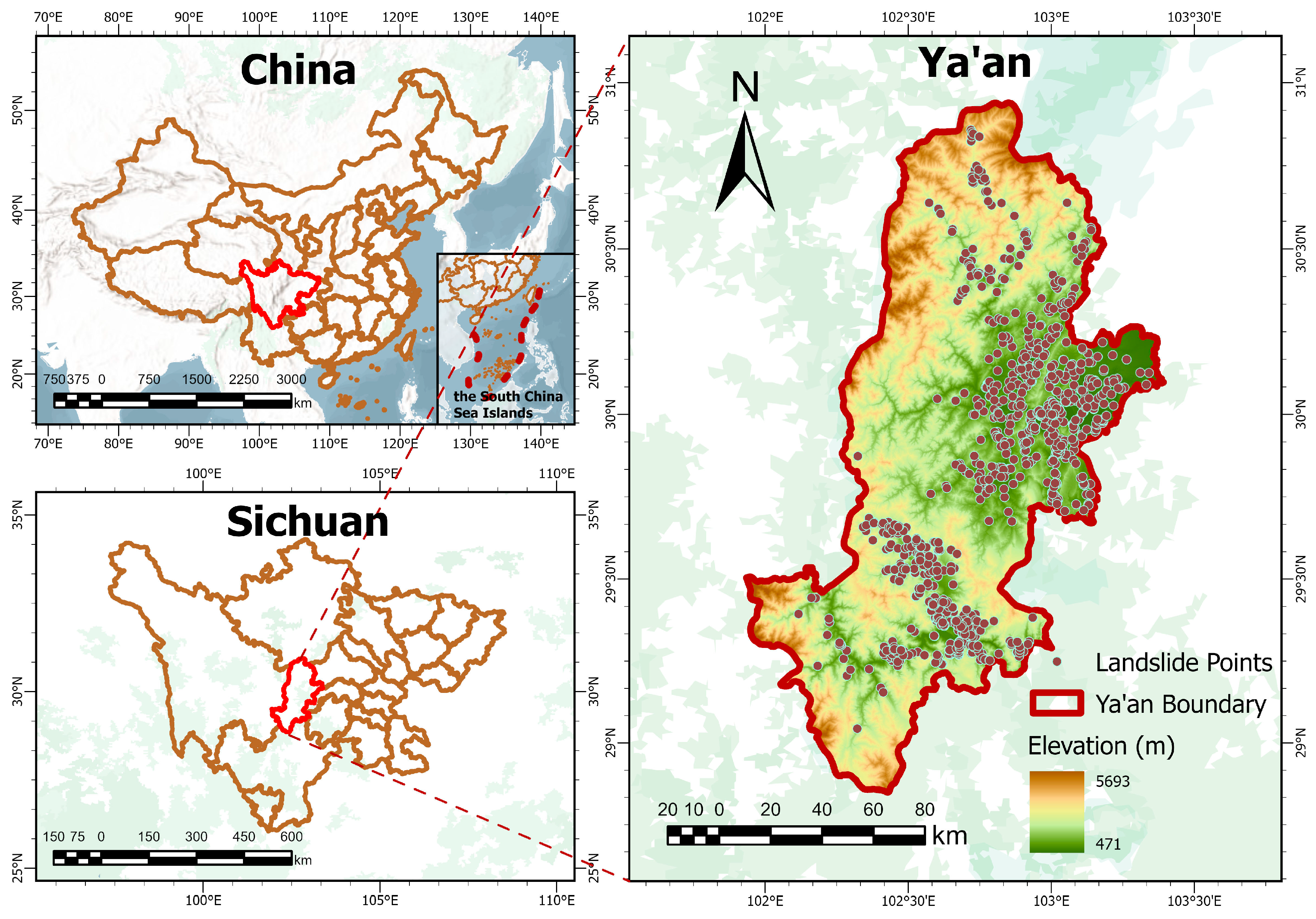
2.1. Study Area
2.2. Data Sources
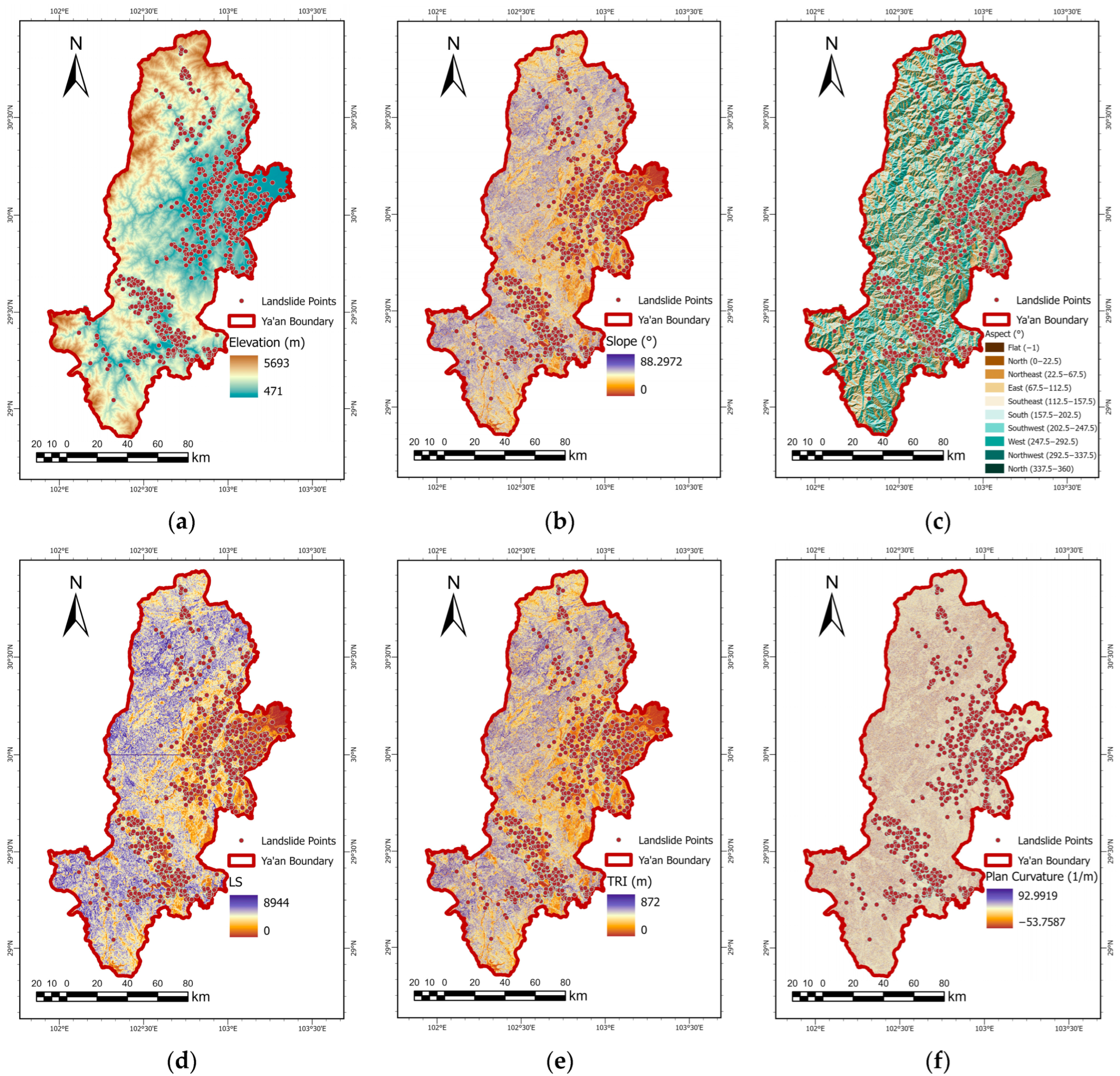
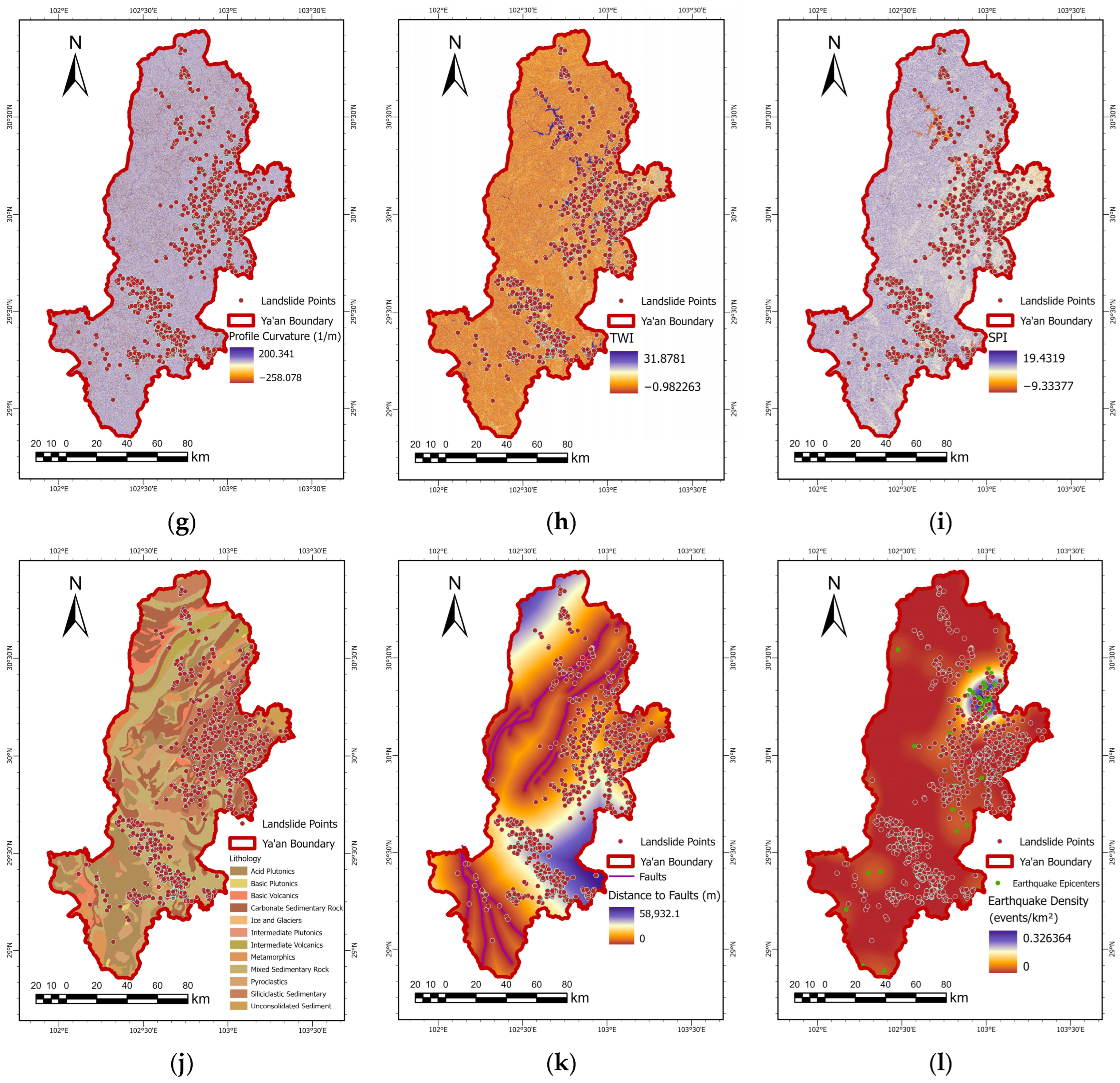
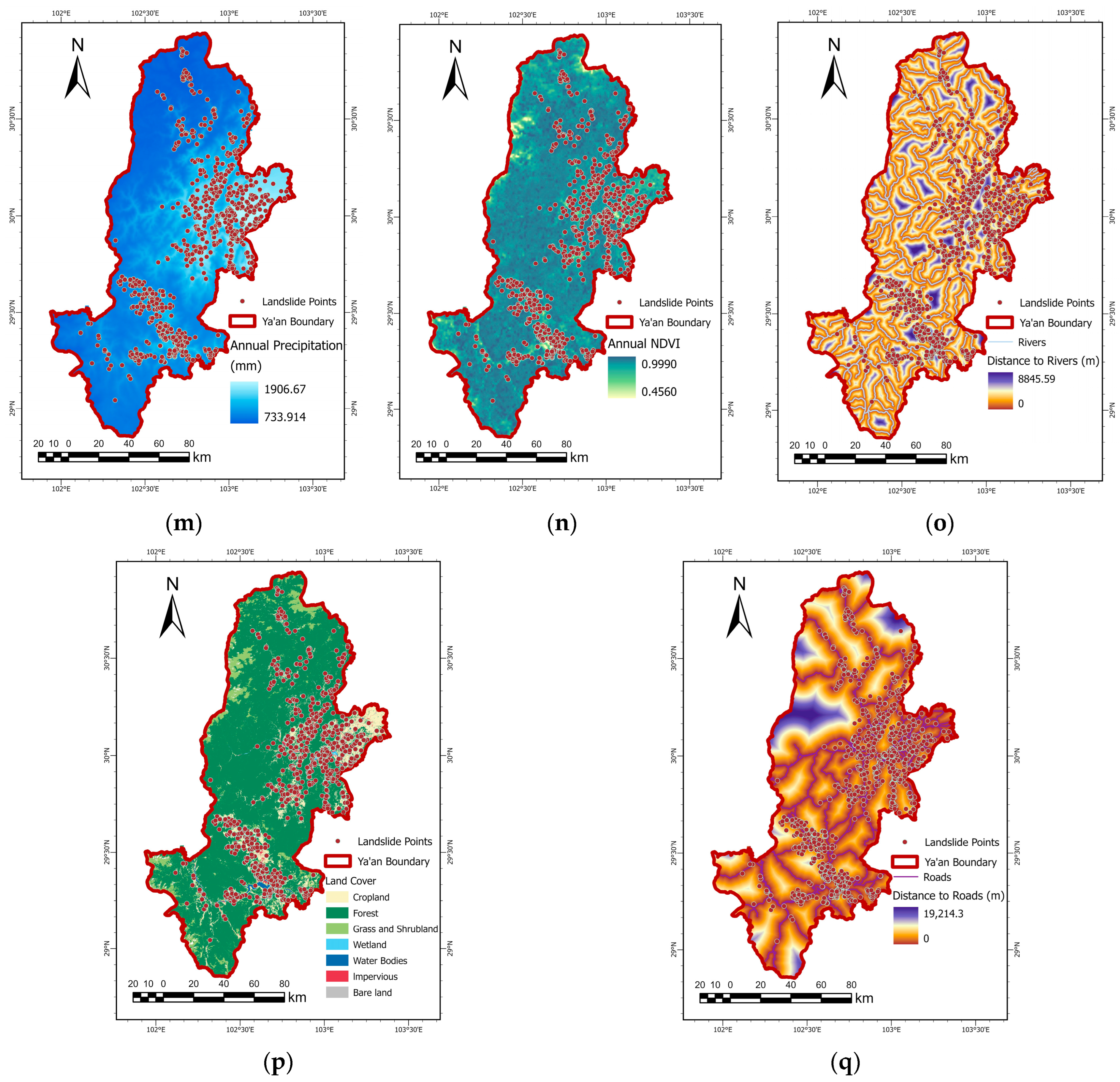
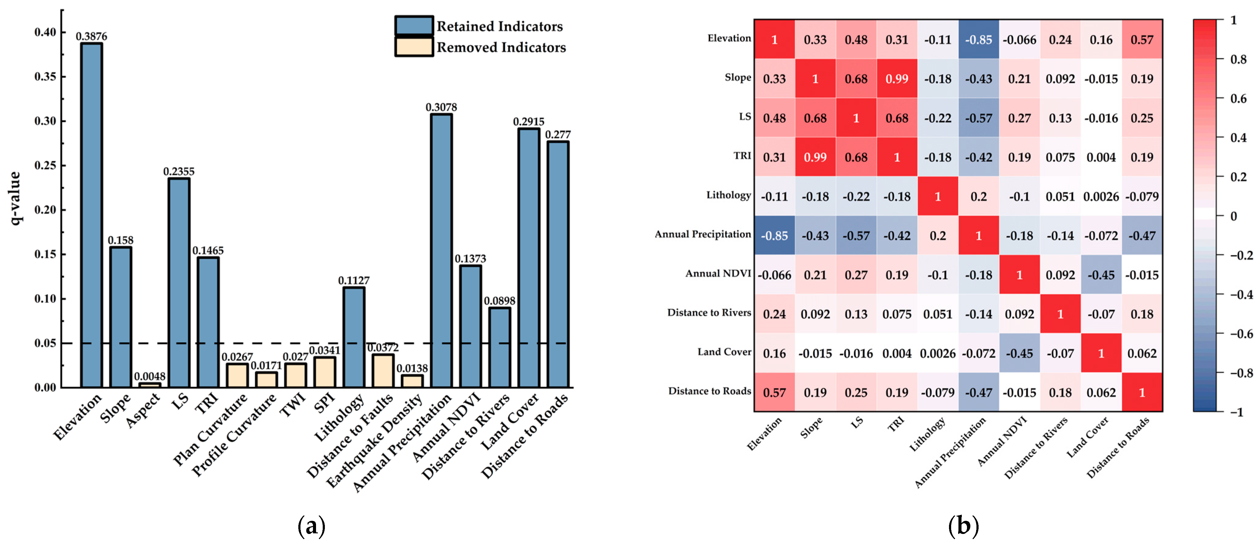
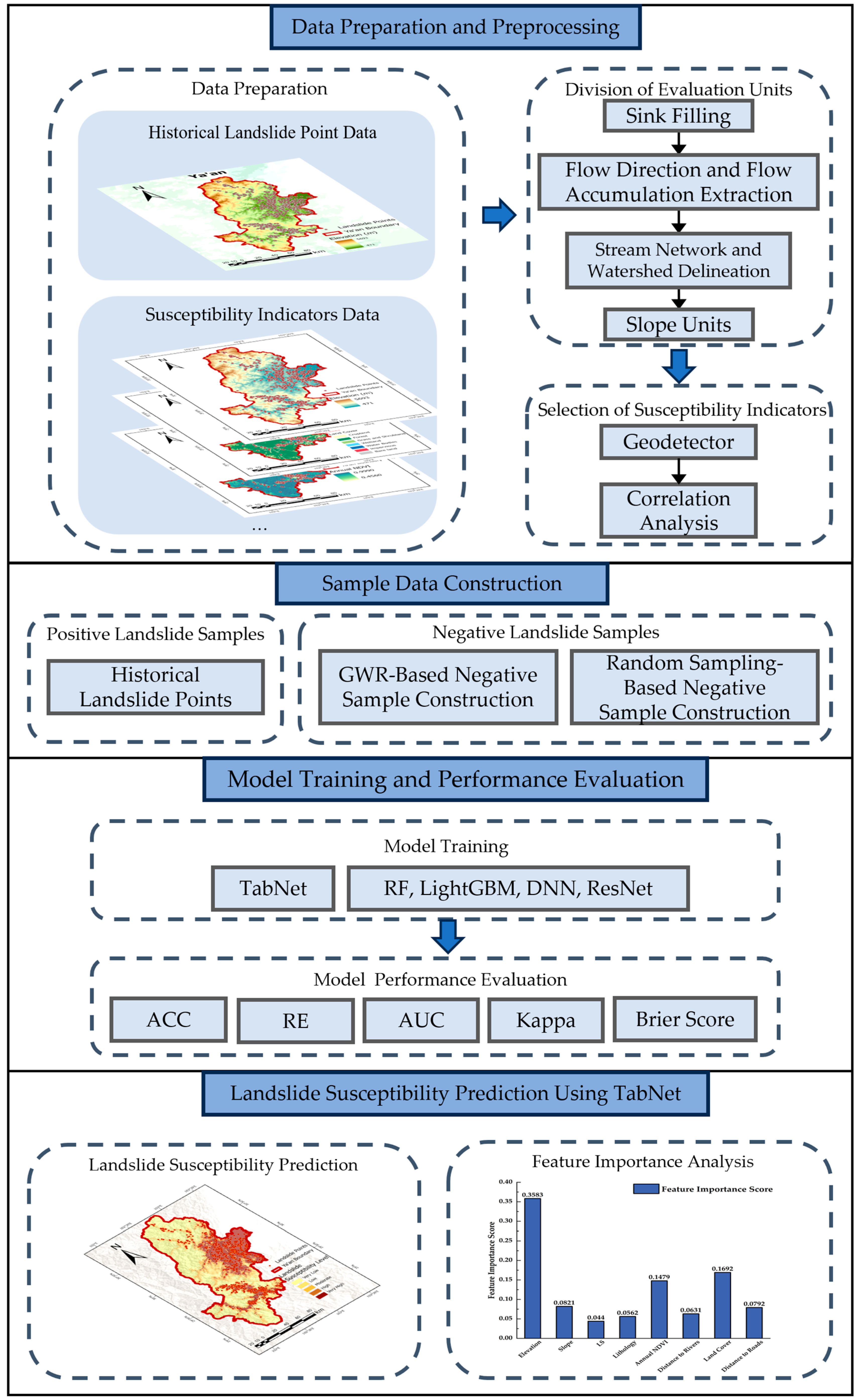
2.3. Division of Evaluation Units and Selection of Susceptibility Indicators
3. Method
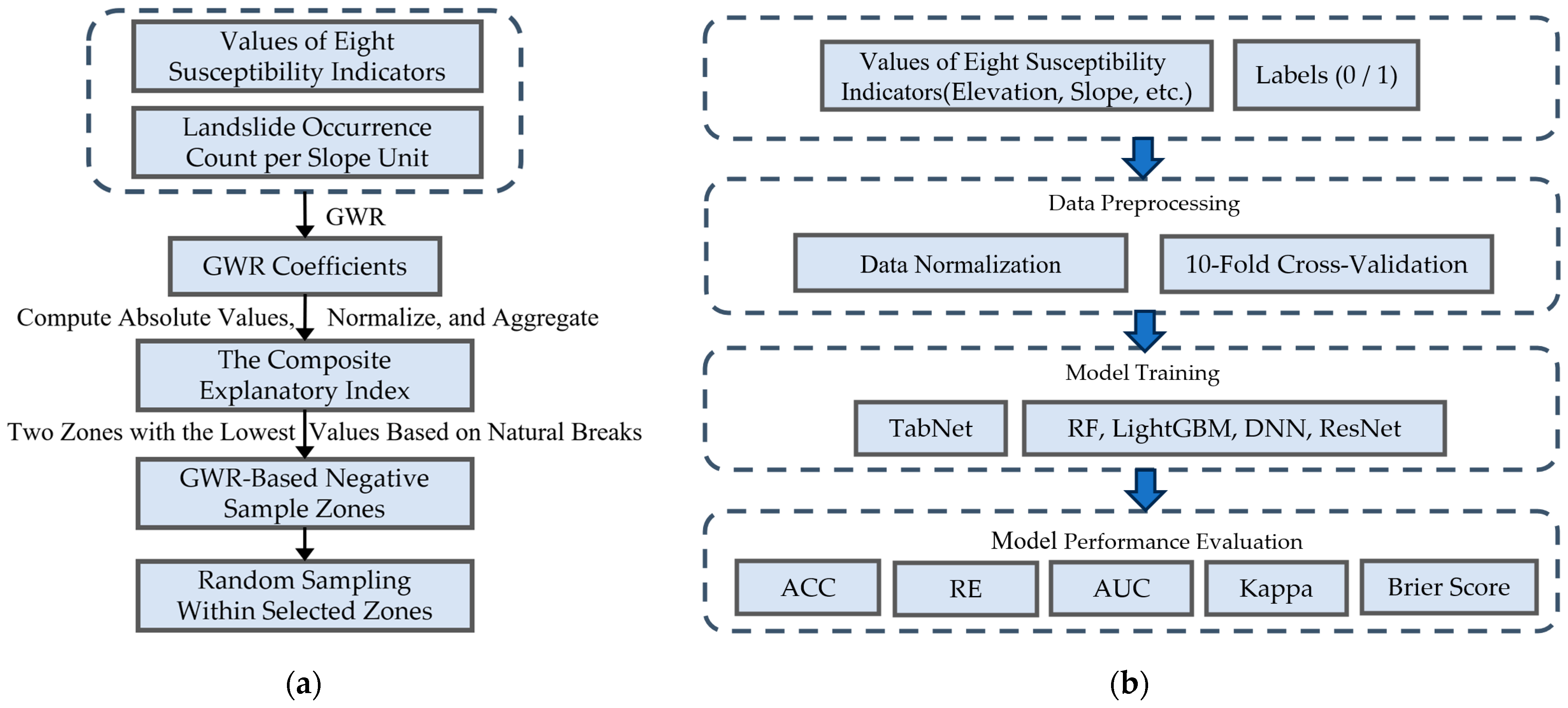
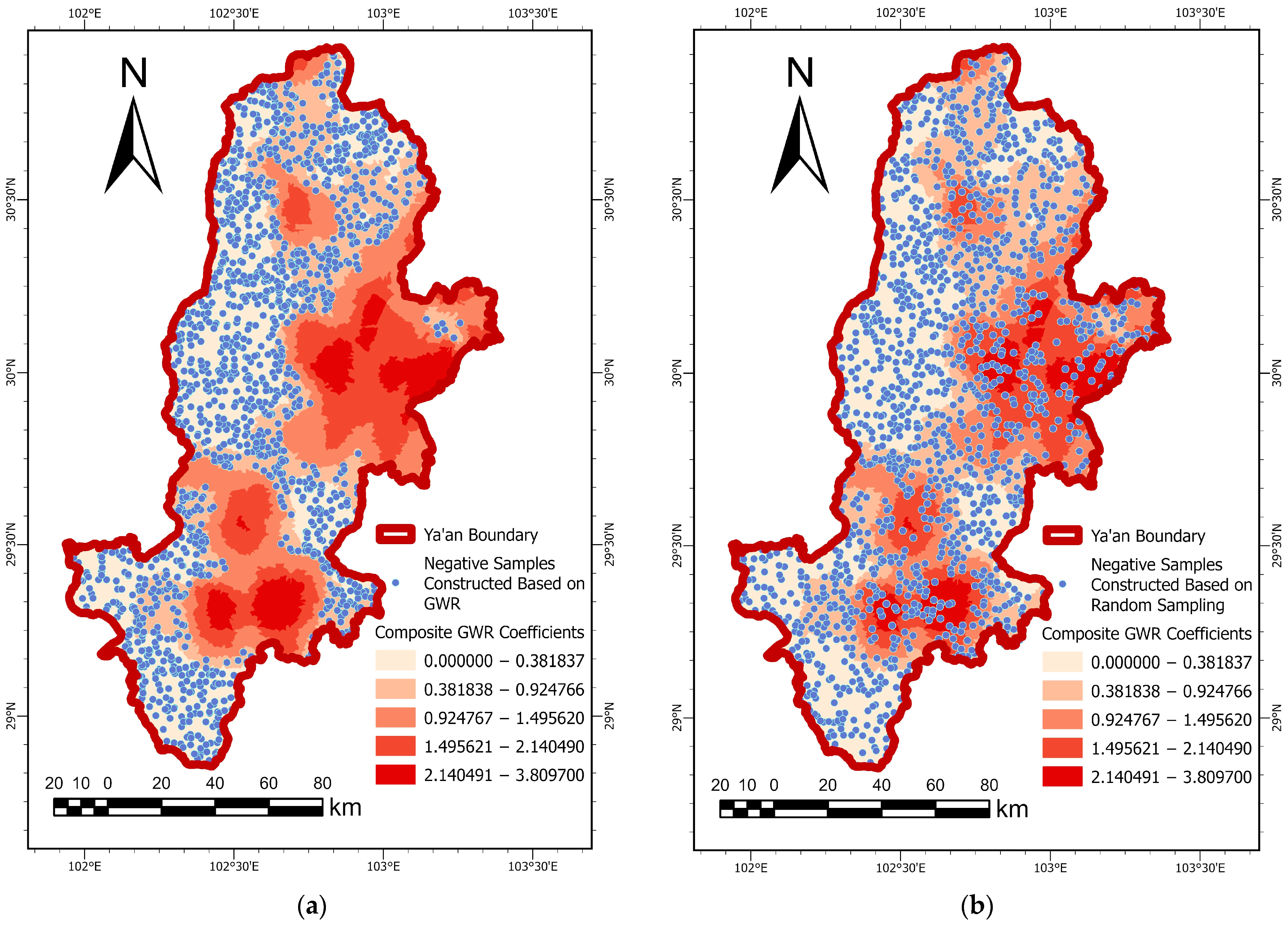
3.1. Negative Sample Construction Based on GWR
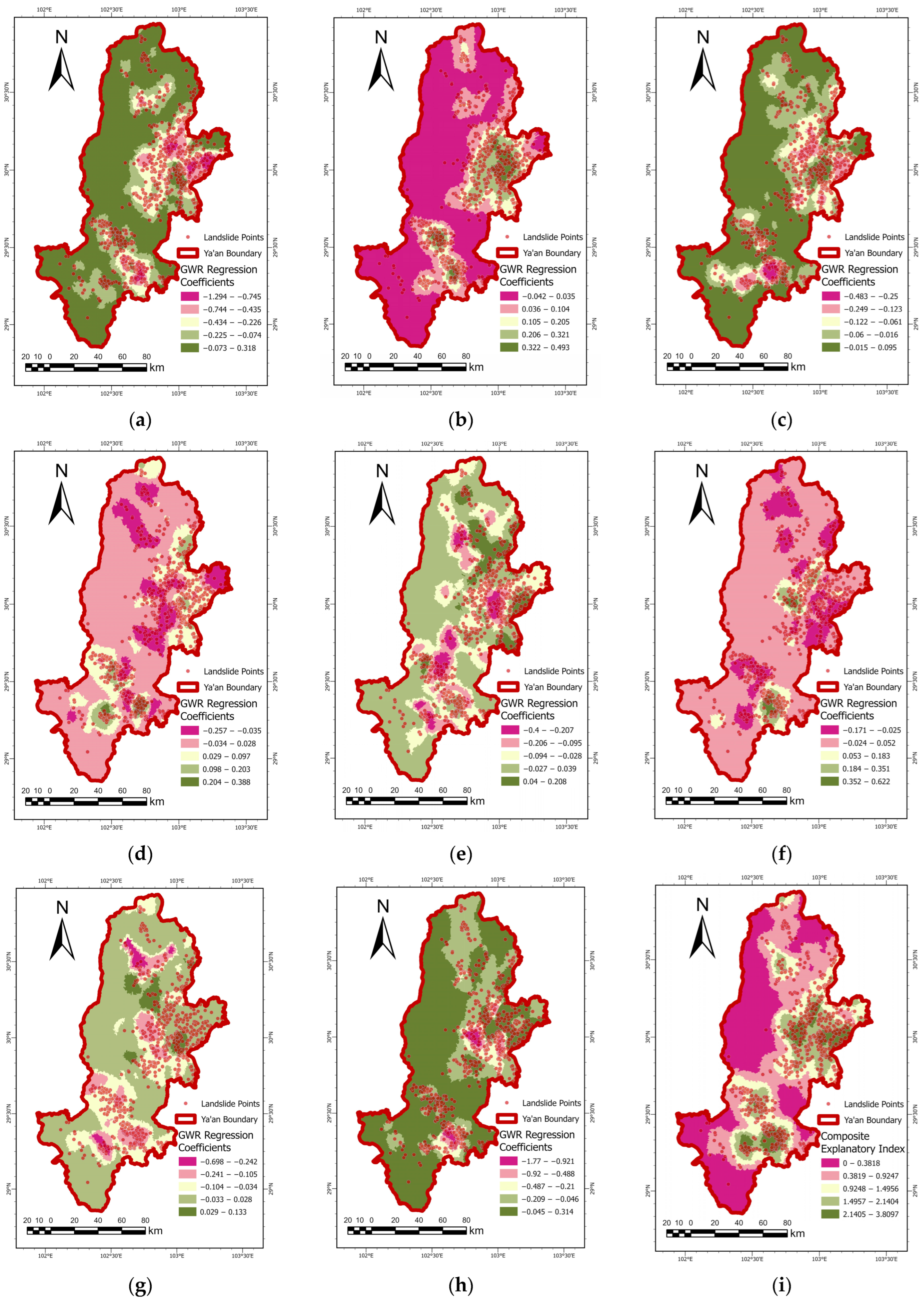
3.1.1. GWR Modeling Principle
3.1.2. Identification of Low-Explanatory Areas and Selection of Negative Samples
3.2. Landslide Susceptibility Modeling Based on TabNet
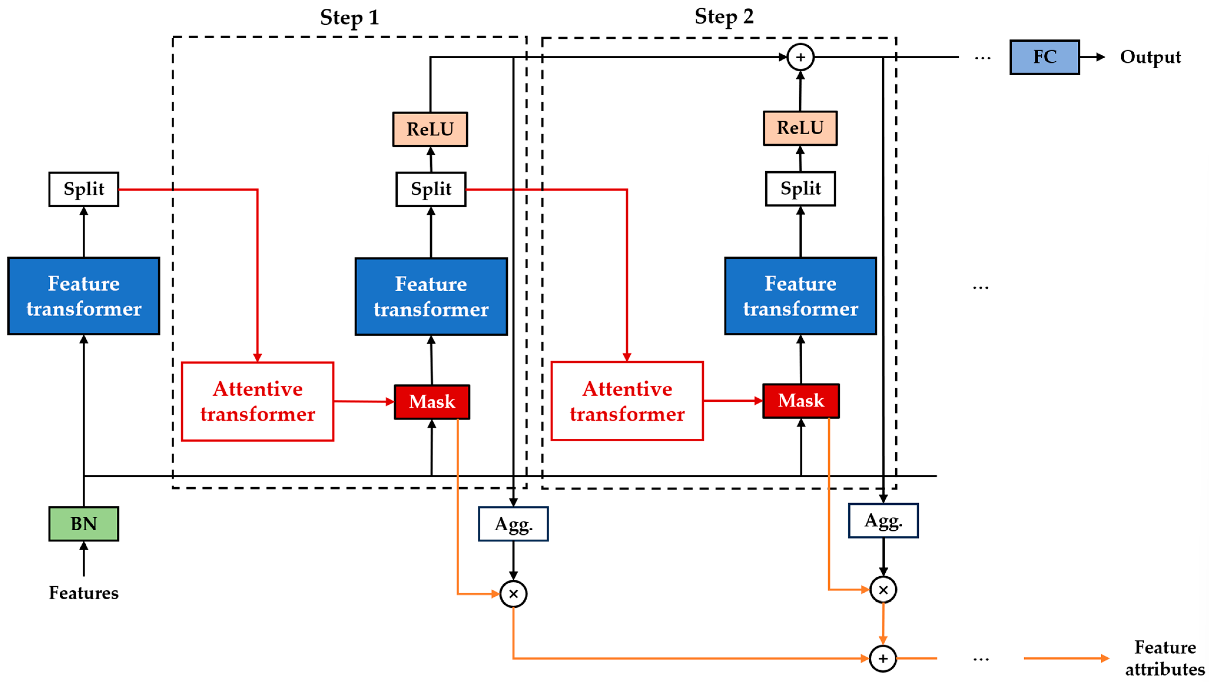
3.2.1. Overview of TabNet
3.2.2. Cross-Validation
3.2.3. Model Performance Evaluation Metrics
4. Results
4.1. Comparison of Results Under Different Negative Sample Construction Strategies
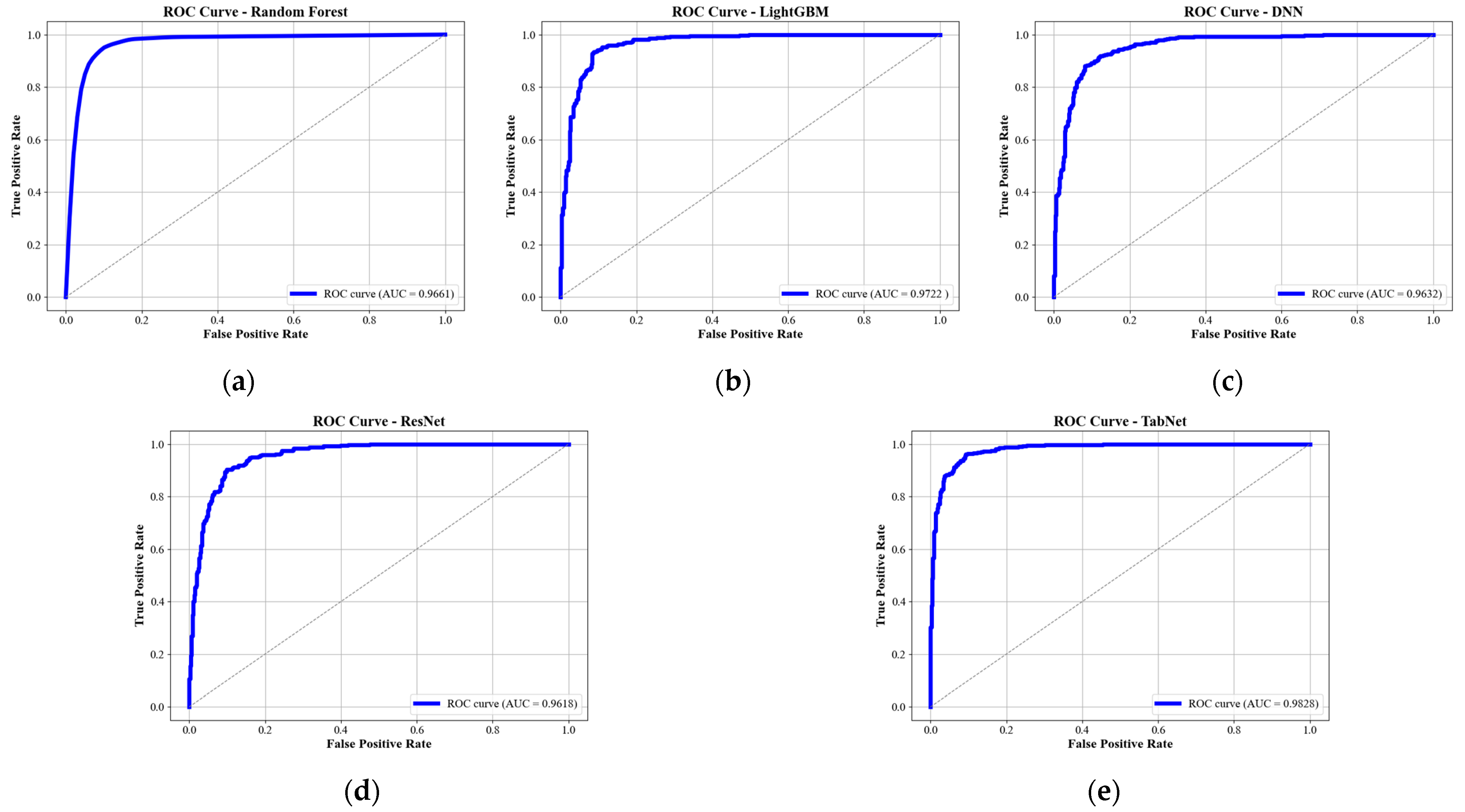
4.2. Comparison of Landslide Susceptibility Modeling Results Across Different Models
4.3. Landslide Susceptibility Prediction and Feature Importance Analysis Based on TabNet
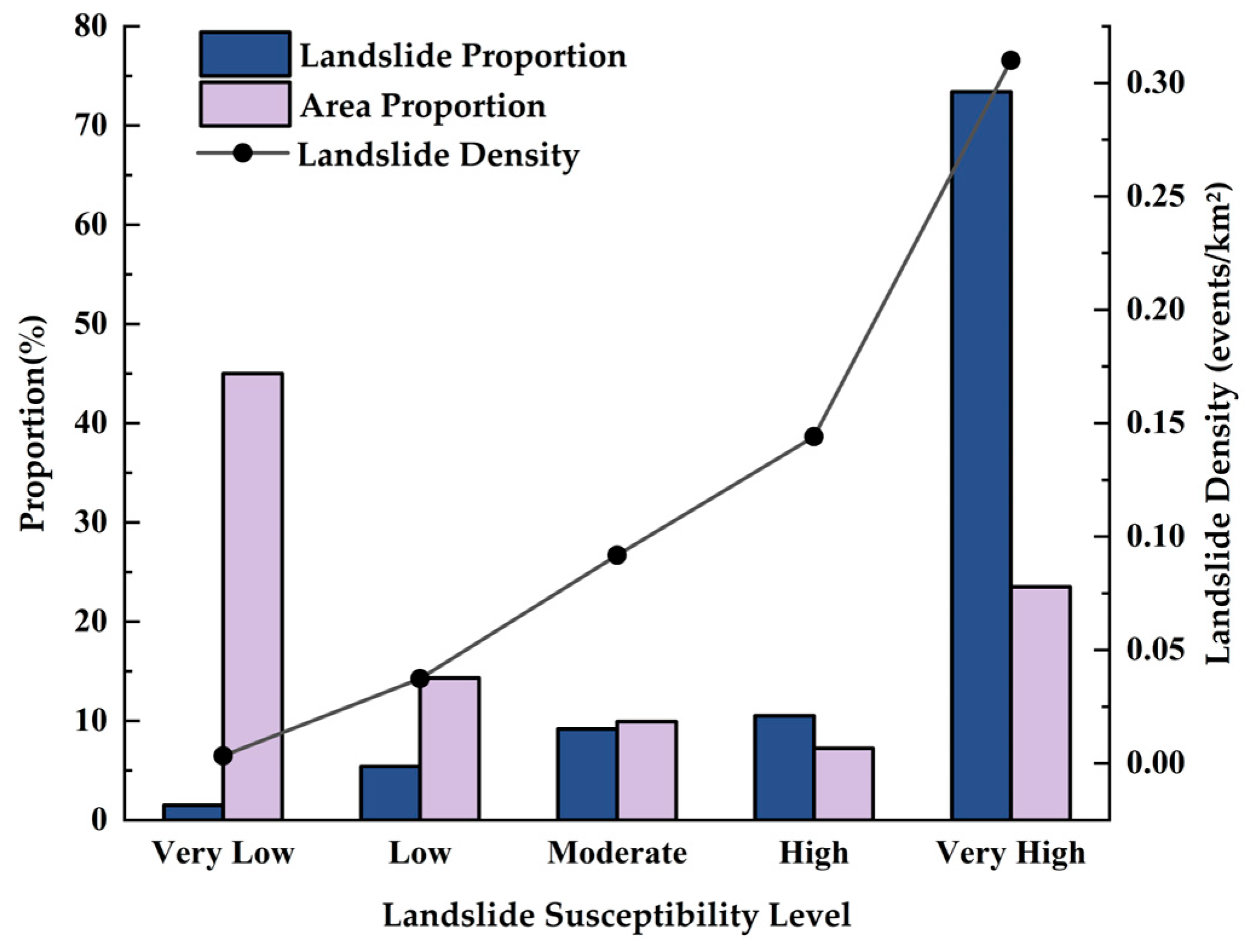
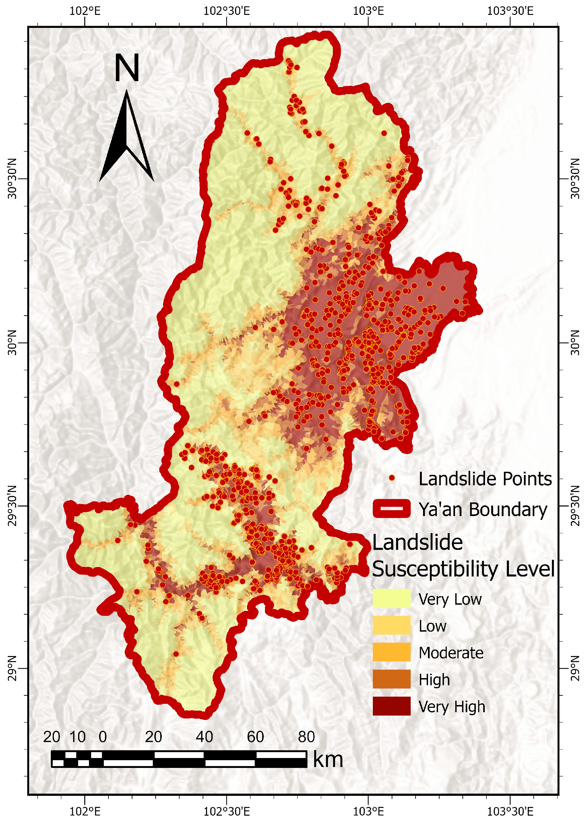
4.3.1. Landslide Susceptibility Prediction
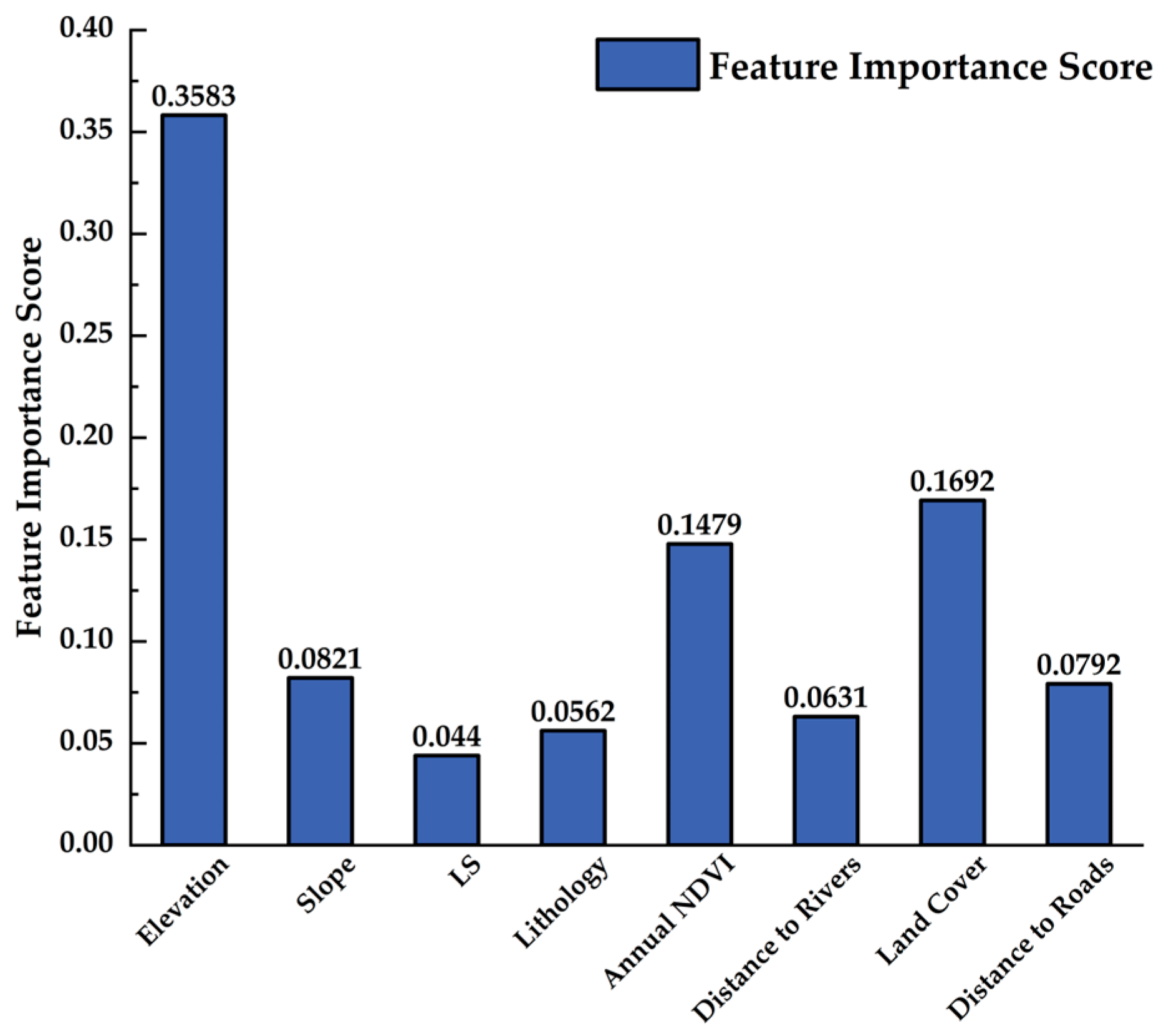
4.3.2. Feature Importance Analysis
5. Discussion
5.1. Rationale and Limitations of GWR-Based Negative Sample Construction
5.2. Evaluating TabNet’s Robustness and Applicability in Susceptibility Modeling
5.3. Relevance and Limitations of Susceptibility Indicators
6. Conclusions
- (1)
- The GWR-based negative sampling method consistently outperforms traditional random sampling across all evaluated models, significantly improving both discriminative accuracy and generalization performance. By selecting negative samples from regions with low composite explanatory power, the GWR approach enhances the representativeness of low-risk areas and improves the distinction between positive and negative instances.
- (2)
- As a deep neural network specifically designed for structured data, TabNet achieves outstanding performance in landslide susceptibility modeling, attaining an average AUC of 0.9828, which is substantially higher than those of RF, LightGBM, DNN, and ResNet. TabNet exhibits strong adaptability to structured inputs, high predictive accuracy, and robust interpretability, confirming its effectiveness and suitability for modeling complex, multi-factor geological hazards.
- (3)
- Feature importance analysis identifies elevation, land cover, and annual NDVI as the most highly influential factors, highlighting the combined effects of topographic conditions, anthropogenic disturbances, and vegetation cover on landslide susceptibility.
Author Contributions
Funding
Data Availability Statement
Conflicts of Interest
References
- Cruden, D. A simple definition of a landslide. Bull. Eng. Geol. Environ. 1991, 43, 27–29. [Google Scholar] [CrossRef]
- Reichenbach, P.; Rossi, M.; Malamud, B.D.; Mihir, M.; Guzzetti, F. A review of statistically-based landslide susceptibility models. Earth-Sci. Rev. 2018, 180, 60–91. [Google Scholar] [CrossRef]
- Pourghasemi, H.R.; Teimoori Yansari, Z.; Panagos, P.; Pradhan, B. Analysis and evaluation of landslide susceptibility: A review on articles published during 2005–2016 (periods of 2005–2012 and 2013–2016). Arab. J. Geosci. 2018, 11, 193. [Google Scholar] [CrossRef]
- Das, S.; Sarkar, S.; Kanungo, D.P. GIS-based landslide susceptibility zonation mapping using the analytic hierarchy process (AHP) method in parts of Kalimpong Region of Darjeeling Himalaya. Environ. Monit. Assess. 2022, 194, 234. [Google Scholar] [CrossRef]
- Bahrami, Y.; Hassani, H.; Maghsoudi, A. Landslide susceptibility mapping using AHP and fuzzy methods in the Gilan province, Iran. GeoJournal 2021, 86, 1797–1816. [Google Scholar] [CrossRef]
- Farooq, S.; Akram, M.S. Landslide susceptibility mapping using information value method in Jhelum Valley of the Himalayas. Arab. J. Geosci. 2021, 14, 824. [Google Scholar] [CrossRef]
- Chen, L.; Guo, H.; Gong, P.; Yang, Y.; Zuo, Z.; Gu, M. Landslide susceptibility assessment using weights-of-evidence model and cluster analysis along the highways in the Hubei section of the Three Gorges Reservoir Area. Comput. Geosci. 2021, 156, 104899. [Google Scholar] [CrossRef]
- Shano, L.; Raghuvanshi, T.K.; Meten, M. Landslide susceptibility mapping using frequency ratio model: The case of Gamo highland, South Ethiopia. Arab. J. Geosci. 2021, 14, 632. [Google Scholar] [CrossRef]
- Pourghasemi, H.R.; Sadhasivam, N.; Amiri, M.; Eskandari, S.; Santosh, M. Landslide susceptibility assessment and mapping using state-of-the art machine learning techniques. Nat. Hazards 2021, 108, 1291–1316. [Google Scholar] [CrossRef]
- Marjanović, M.; Kovačević, M.; Bajat, B.; Voženílek, V. Landslide susceptibility assessment using SVM machine learning algorithm. Eng. Geol. 2011, 123, 225–234. [Google Scholar] [CrossRef]
- Tien Bui, D.; Tuan, T.A.; Klempe, H.; Pradhan, B.; Revhaug, I. Spatial prediction models for shallow landslide hazards: A comparative assessment of the efficacy of support vector machines, artificial neural networks, kernel logistic regression, and logistic model tree. Landslides 2016, 13, 361–378. [Google Scholar] [CrossRef]
- Trigila, A.; Iadanza, C.; Esposito, C.; Scarascia-Mugnozza, G. Comparison of Logistic Regression and Random Forests techniques for shallow landslide susceptibility assessment in Giampilieri (NE Sicily, Italy). Geomorphology 2015, 249, 119–136. [Google Scholar] [CrossRef]
- Sun, D.; Wu, X.; Wen, H.; Gu, Q. A LightGBM-based landslide susceptibility model considering the uncertainty of non-landslide samples. Geomat. Nat. Hazards Risk 2023, 14, 2213807. [Google Scholar] [CrossRef]
- L’heureux, A.; Grolinger, K.; Elyamany, H.F.; Capretz, M.A. Machine learning with big data: Challenges and approaches. IEEE Access 2017, 5, 7776–7797. [Google Scholar] [CrossRef]
- Azarafza, M.; Azarafza, M.; Akgün, H.; Atkinson, P.M.; Derakhshani, R. Deep learning-based landslide susceptibility mapping. Sci. Rep. 2021, 11, 24112. [Google Scholar] [CrossRef]
- Wang, Y.; Fang, Z.; Hong, H. Comparison of convolutional neural networks for landslide susceptibility mapping in Yanshan County, China. Sci. Total Environ. 2019, 666, 975–993. [Google Scholar] [CrossRef]
- Isazade, V.; Qasimi, A.b.; Namivandi, M.S.; Amin, M.S.; Ahlem, G. Landslide Susceptibility Assessment Using Recurrent Neural Network (RNN)—A Case of Chabahar and Konarak in Iran. Indian Geotech. J. 2025, 55, 1–21. [Google Scholar] [CrossRef]
- Xiao, L.; Zhang, Y.; Peng, G. Landslide susceptibility assessment using integrated deep learning algorithm along the China-Nepal highway. Sensors 2018, 18, 4436. [Google Scholar] [CrossRef] [PubMed]
- Liu, T.; Chen, T.; Niu, R.; Plaza, A. Landslide detection mapping employing CNN, ResNet, and DenseNet in the three gorges reservoir, China. IEEE J. Sel. Top. Appl. Earth Obs. Remote Sens. 2021, 14, 11417–11428. [Google Scholar] [CrossRef]
- Ghorbanzadeh, O.; Crivellari, A.; Ghamisi, P.; Shahabi, H.; Blaschke, T. A comprehensive transferability evaluation of U-Net and ResU-Net for landslide detection from Sentinel-2 data (case study areas from Taiwan, China, and Japan). Sci. Rep. 2021, 11, 14629. [Google Scholar] [CrossRef]
- Arik, S.Ö.; Pfister, T. Tabnet: Attentive interpretable tabular learning. In Proceedings of the AAAI Conference on Artificial Intelligence, Virtual, 2–9 February 2021; pp. 6679–6687. [Google Scholar]
- Yu, C.; Jin, Y.; Xing, Q.; Zhang, Y.; Guo, S.; Meng, S. Advanced user credit risk prediction model using lightgbm, xgboost and tabnet with smoteenn. In Proceedings of the 2024 IEEE 6th International Conference on Power, Intelligent Computing and Systems (ICPICS), Shenyang, China, 26–28 July 2024; pp. 876–883. [Google Scholar]
- Joseph, L.P.; Joseph, E.A.; Prasad, R. Explainable diabetes classification using hybrid Bayesian-optimized TabNet architecture. Comput. Biol. Med. 2022, 151, 106178. [Google Scholar] [CrossRef] [PubMed]
- Yan, J.; Xu, T.; Yu, Y.; Xu, H. Rainfall forecast model based on the tabnet model. Water 2021, 13, 1272. [Google Scholar] [CrossRef]
- Shah, C.; Du, Q.; Xu, Y. Enhanced TabNet: Attentive interpretable tabular learning for hyperspectral image classification. Remote Sens. 2022, 14, 716. [Google Scholar] [CrossRef]
- Zhu, Y.; Liu, S.; Yin, K.; Zeng, T.; Guo, Z.; Liu, Z.; Yang, H. Impact of negative sampling strategies on landslide susceptibility assessment. Adv. Space Res. 2025, 76, 592–613. [Google Scholar] [CrossRef]
- Fotheringham, A.S.; Brunsdon, C.; Charlton, M. Geographically weighted regression. Sage Handb. Spat. Anal. 2009, 1, 243–254. [Google Scholar]
- Li, Y.; Liu, X.; Han, Z.; Dou, J. Spatial proximity-based geographically weighted regression model for landslide susceptibility assessment: A case study of Qingchuan area, China. Appl. Sci. 2020, 10, 1107. [Google Scholar] [CrossRef]
- Xueqiang, G.; Chuanjie, X.; Xiewen, H.; Yayun, H.; Yonghao, Z.; Yu, Z. Landslide susceptibility assessment and zonation using negative sampling strategy: A case study of Bazhong area, Sichuan Province. Chin. J. Geol. Hazard Control 2025, 36, 146. [Google Scholar]
- McCool, D.; Foster, G.; Weesies, G. Slope length and steepness factors (LS). In Predicting Soil Erosion by Water: A Guide to Conservation Planning with the Revised Universal Soil Loss Equation (RUSLE); US Department of Agriculture: Washington, DC, USA, 1997; Volume 703, pp. 101–141. [Google Scholar]
- Riley, S.J.; DeGloria, S.D.; Elliot, R. Index that quantifies topographic heterogeneity. Intermt. J. Sci. 1999, 5, 23–27. [Google Scholar]
- Wilson, J.P.; Gallant, J.C. Primary topographic attributes. In Terrain Analysis-Principles and Application; John Wiley & Sons: Hoboken, NJ, USA, 2000; pp. 51–86. [Google Scholar]
- Zevenbergen, L.W.; Thorne, C.R. Quantitative analysis of land surface topography. Earth Surf. Process. Landf. 1987, 12, 47–56. [Google Scholar] [CrossRef]
- Beven, K.J.; Kirkby, M.J. A physically based, variable contributing area model of basin hydrology/Un modèle à base physique de zone d’appel variable de l’hydrologie du bassin versant. Hydrol. Sci. J. 1979, 24, 43–69. [Google Scholar] [CrossRef]
- Moore, I.D.; Grayson, R.; Ladson, A. Digital terrain modelling: A review of hydrological, geomorphological, and biological applications. Hydrol. Process. 1991, 5, 3–30. [Google Scholar] [CrossRef]
- Rouse, J.; Haas, R.; Schell, J.; Deering, D. Monitoring vegetation systems in the great plains with ERTS proceeding. In Proceedings of the Third Earth Reserves Technology Satellite Symposium, Washington, DC, USA, 1 January 1974; p. 317. [Google Scholar]
- Yu, X.; Chen, H. Research on the influence of different sampling resolution and spatial resolution in sampling strategy on landslide susceptibility mapping results. Sci. Rep. 2024, 14, 1549. [Google Scholar] [CrossRef] [PubMed]
- Meena, S.R.; Gudiyangada Nachappa, T. Impact of spatial resolution of digital elevation model on landslide susceptibility mapping: A case study in Kullu Valley, Himalayas. Geosciences 2019, 9, 360. [Google Scholar] [CrossRef]
- Jacobs, L.; Kervyn, M.; Reichenbach, P.; Rossi, M.; Marchesini, I.; Alvioli, M.; Dewitte, O. Regional susceptibility assessments with heterogeneous landslide information: Slope unit-vs. pixel-based approach. Geomorphology 2020, 356, 107084. [Google Scholar] [CrossRef]
- Tian, S.; Zhang, S.; Tang, Q.; Fan, X.; Han, P. Comparative study of landslide susceptibility assessment based on different evaluation units. J. Nat. Disasters 2019, 2019, 137–145. [Google Scholar]
- Shang, H.; Ni, W.; Cheng, H. Application of slope unit division to risk zoning of geological hazards of Pengyang County. Soil Water Conserv. China 2011, 3, 48–50. [Google Scholar]
- Liu, Y.; Zhang, W.; Zhang, Z.; Xu, Q.; Li, W. Risk factor detection and landslide susceptibility mapping using Geo-Detector and Random Forest Models: The 2018 Hokkaido eastern Iburi earthquake. Remote Sens. 2021, 13, 1157. [Google Scholar] [CrossRef]
- Wang, J.-F.; Zhang, T.-L.; Fu, B.-J. A measure of spatial stratified heterogeneity. Ecol. Indic. 2016, 67, 250–256. [Google Scholar] [CrossRef]
- Gu, T.; Li, J.; Wang, M.; Duan, P.; Zhang, Y.; Cheng, L. Study on landslide susceptibility mapping with different factor screening methods and random forest models. PLoS ONE 2023, 18, e0292897. [Google Scholar] [CrossRef]
- Zhang, Q.; He, Y.; Chen, X.; Gao, B.; Zhang, L.; Zhang, Z.; Lu, J.; Zhang, Y. Landslide susceptibility assessment in Shenzhen based on multi-scale convolutional neural networks model. Chin. J. Geol. Hazard Control 2024, 35, 146–162. [Google Scholar]
- Zou, K.H.; Tuncali, K.; Silverman, S.G. Correlation and simple linear regression. Radiology 2003, 227, 617–628. [Google Scholar] [CrossRef]
- Krehbiel, T.C. Correlation Coefficient Rule of Thumb. Decis. Sci. J. Innov. Educ. 2004, 2, 97. [Google Scholar] [CrossRef]
- Jenks, G.F. The data model concept in statistical mapping. Int. Yearb. Cartogr. 1967, 7, 186–190. [Google Scholar]
- An, B.; Zhang, Z.; Xiong, S.; Zhang, W.; Yi, Y.; Liu, Z.; Liu, C. Landslide Susceptibility Mapping Based on Ensemble Learning in the Jiuzhaigou Region, Sichuan, China. Remote Sens. 2024, 16, 4218. [Google Scholar] [CrossRef]
- Arabameri, A.; Saha, S.; Roy, J.; Chen, W.; Blaschke, T.; Tien Bui, D. Landslide susceptibility evaluation and management using different machine learning methods in the Gallicash River Watershed, Iran. Remote Sens. 2020, 12, 475. [Google Scholar] [CrossRef]
- Meier, C.; Jaboyedoff, M.; Derron, M.-H.; Gerber, C. A method to assess the probability of thickness and volume estimates of small and shallow initial landslide ruptures based on surface area. Landslides 2020, 17, 975–982. [Google Scholar] [CrossRef]
- Breiman, L. Random forests. Mach. Learn. 2001, 45, 5–32. [Google Scholar] [CrossRef]
- Ke, G.; Meng, Q.; Finley, T.; Wang, T.; Chen, W.; Ma, W.; Ye, Q.; Liu, T.-Y. Lightgbm: A highly efficient gradient boosting decision tree. Adv. Neural Inf. Process. Syst. 2017, 30, 52. [Google Scholar]
- Hinton, G.E.; Osindero, S.; Teh, Y.-W. A fast learning algorithm for deep belief nets. Neural Comput. 2006, 18, 1527–1554. [Google Scholar] [CrossRef]
- He, K.; Zhang, X.; Ren, S.; Sun, J. Deep residual learning for image recognition. In Proceedings of the IEEE Conference on Computer Vision and Pattern Recognition, Las Vegas, NV, USA, 27–30 June 2016; pp. 770–778. [Google Scholar]
- Refaeilzadeh, P.; Tang, L.; Liu, H. Cross-validation. In Encyclopedia of Database Systems; Springer: New York, NY, USA, 2009; pp. 532–538. [Google Scholar]
- Kuhn, M.; Johnson, K. Applied Predictive Modeling; Springer: New York, NY, USA, 2013; Volume 26. [Google Scholar]
- Dai, X.; Zhu, Y.; Sun, K.; Zou, Q.; Zhao, S.; Li, W.; Hu, L.; Wang, S. Examining the spatially varying relationships between landslide susceptibility and conditioning factors using a geographical random forest approach: A case study in Liangshan, China. Remote Sens. 2023, 15, 1513. [Google Scholar] [CrossRef]
- Brenning, A. Spatial prediction models for landslide hazards: Review, comparison and evaluation. Nat. Hazards Earth Syst. Sci. 2005, 5, 853–862. [Google Scholar] [CrossRef]
- Cohen, J. A coefficient of agreement for nominal scales. Educ. Psychol. Meas. 1960, 20, 37–46. [Google Scholar] [CrossRef]
- Glenn, W.B. Verification of forecasts expressed in terms of probability. Mon. Weather. Rev. 1950, 78, 1–3. [Google Scholar]
- Landis, J.R.; Koch, G.G. The measurement of observer agreement for categorical data. Biometrics 1977, 33, 159–174. [Google Scholar] [CrossRef] [PubMed]
- Getis, A.; Ord, J.K. The analysis of spatial association by use of distance statistics. Geogr. Anal. 1992, 24, 189–206. [Google Scholar] [CrossRef]
- Manap, N.; Borhan, M.N.; Yazid, M.R.M.; Hambali, M.K.A.; Rohan, A. Determining spatial patterns of road accidents at expressway by applying Getis-Ord Gi* spatial statistic. Int. J. Recent Technol. Eng. 2019, 8, 345–350. [Google Scholar] [CrossRef]
- Guo, Z.; Tian, B.; Zhu, Y.; He, J.; Zhang, T. How do the landslide and non-landslide sampling strategies impact landslide susceptibility assessment?—A catchment-scale case study from China. J. Rock Mech. Geotech. Eng. 2024, 16, 877–894. [Google Scholar]
- Kavzoglu, T.; Sahin, E.K.; Colkesen, I. Landslide susceptibility mapping using GIS-based multi-criteria decision analysis, support vector machines, and logistic regression. Landslides 2014, 11, 425–439. [Google Scholar] [CrossRef]
- Dou, H.; He, J.; Huang, S.; Jian, W.; Guo, C. Influences of non-landslide sample selection strategies on landslide susceptibility mapping by machine learning. Geomat. Nat. Hazards Risk 2023, 14, 2285719. [Google Scholar] [CrossRef]
- Xiaoting, Z.; Faming, H.; Weicheng, W.; Chuangbing, Z.; Shiyi, Z.; Lihan, P. Regional Landslide Susceptibility Prediction Based on Negative Sample Selected by Coupling Information Value Method. Adv. Eng. Sci./Gongcheng Kexue Yu Jishu 2022, 54, 25. [Google Scholar]
- Wang, Y.; Feng, L.; Li, S.; Ren, F.; Du, Q. A hybrid model considering spatial heterogeneity for landslide susceptibility mapping in Zhejiang Province, China. Catena 2020, 188, 104425. [Google Scholar] [CrossRef]
- Huang, F.; Chen, J.; Liu, W.; Huang, J.; Hong, H.; Chen, W. Regional rainfall-induced landslide hazard warning based on landslide susceptibility mapping and a critical rainfall threshold. Geomorphology 2022, 408, 108236. [Google Scholar] [CrossRef]

| Data Type | Data Name | Resolution | Data Source |
|---|---|---|---|
| Historical Landslide Point Data | Spatial Distribution Data of Geological Hazard Points in China | - | Resource and Environmental Science Data Platform |
| Elevation Data | ASTER GDEM Data of Ya’an City | 30 m | Geospatial Data Cloud site |
| LS Data | Slope Length and Steepness Factor Dataset for the 20 Countries of the Pan-Third Pole Region | 7.5 arc-s | National Tibetan Plateau Data Center |
| Lithology Data | Spatial Lithology Distribution Data of China | 7.5 arc-s | Resource and Environmental Science Data Platform |
| Fault Vector Data | Vector Data of Active Faults in China | - | Seismic Active Fault Survey Data Center |
| Earthquake Epicenter Data | Global Earthquake Data (2000–2022) | - | United States Geological Survey |
| Annual Precipitation Data | Annual Precipitation Data of China (2000–2022) | 1 km | National Earth System Science Data Center |
| River and Road Vector Data | Fundamental Geographic Information Data of China | - | National Geomatics Center of China |
| Annual NDVI Data | Annual Average NDVI Data of China (2000–2022) | 1 km | Resource and Environmental Science Data Platform |
| Land Cover Data | Land Cover Data of China | 30 m | National Geomatics Center of China |
| Metric | Formula * | Definition |
|---|---|---|
| ACC | Proportion of correctly identified landslide and non-landslide units. | |
| RE | Proportion of actual landslide units that are correctly classified as landslides. | |
| ROC | Plot of TPR vs. FPR | Reflects the model’s ability to distinguish landslide from non-landslide areas; the closer the curve is to the top-left corner, the better the performance. |
| AUC | Area under the ROC curve | Quantifies the model’s discrimination ability; values closer to 1 indicate stronger performance. |
| Kappa | Measures agreement between the true classes and the classifications; values closer to 1 indicate stronger consistency, while values near 0 or negative suggest performance equivalent to random guessing, or indicate systematic bias. | |
| Brier Score | Measures the mean squared difference between predicted probabilities and actual outcomes; lower scores reflect more reliable probabilistic predictions [62]. |
| Negative Samples Selected Based on Random Sampling | Negative Samples Selected Based on GWR | |
|---|---|---|
| RF | 0.9300 | 0.9661 |
| LightGBM | 0.9333 | 0.9722 |
| DNN | 0.9022 | 0.9632 |
| ResNet | 0.9029 | 0.9618 |
| TabNet | 0.9456 | 0.9828 |
| ACC | RE | AUC | Kappa | Brier Score | |
|---|---|---|---|---|---|
| RF | 0.9281 | 0.9489 | 0.9661 | 0.8558 | 0.0601 |
| LightGBM | 0.9207 | 0.9195 | 0.9722 | 0.8409 | 0.0614 |
| DNN | 0.9046 | 0.8974 | 0.9632 | 0.8083 | 0.0720 |
| ResNet | 0.8992 | 0.8903 | 0.9618 | 0.7977 | 0.0735 |
| TabNet | 0.9298 | 0.9196 | 0.9828 | 0.8589 | 0.0521 |
| Susceptibility Level | Landslide Count | Landslide Proportion (%) | Area (km2) | Area Proportion (%) | Landslide Density (Events/km2) |
|---|---|---|---|---|---|
| Very Low | 22 | 1.49 | 6716.32 | 45.00 | 0.0033 |
| Low | 80 | 5.40 | 2137.48 | 14.32 | 0.0374 |
| Moderate | 136 | 9.18 | 1481.74 | 9.93 | 0.0918 |
| High | 156 | 10.53 | 1082.48 | 7.25 | 0.1441 |
| Very High | 1087 | 73.40 | 3506.67 | 23.50 | 0.3100 |
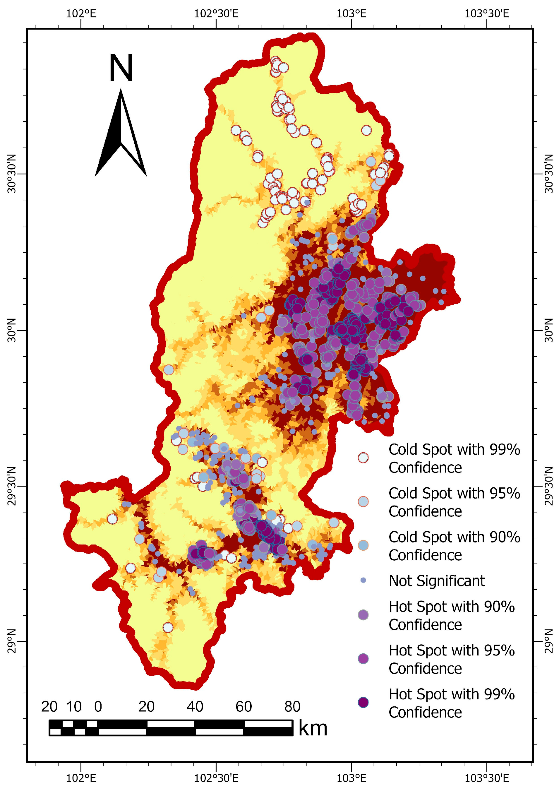
| Gi Bin Value * | p-Value | Meaning | Count | Proportion (%) |
|---|---|---|---|---|
| 3 | p < 0.01 | 99% Confidence Hotspot | 349 | 23.57 |
| 2 | 0.01 ≤ p < 0.05 | 95% Confidence Hotspot | 376 | 25.39 |
| 1 | 0.05 ≤ p < 0.10 | 90% Confidence Hotspot | 87 | 5.87 |
| 0 | p ≥ 0.10 | Not Significant | 428 | 28.9 |
| −1 | 0.05 ≤ p < 0.10 | 90% Confidence Cold Spot | 12 | 0.81 |
| −2 | 0.01 ≤ p < 0.05 | 95% Confidence Cold Spot | 41 | 2.77 |
| −3 | p < 0.01 | 99% Confidence Cold Spot | 188 | 12.69 |
| Susceptibility Level | Landslide Count | Hotspot Count | Hotspot Proportion (%) | Cold Spot Count | Cold Spot Proportion (%) |
|---|---|---|---|---|---|
| Very Low | 22 | 0 | 0 | 20 | 90.91 |
| Low | 80 | 0 | 0 | 75 | 93.75 |
| Moderate | 136 | 5 | 3.68 | 102 | 75 |
| High | 156 | 16 | 10.26 | 26 | 16.67 |
| Very High | 1087 | 791 | 72.77 | 18 | 1.66 |
| Hyperparameter | Description | Tested Range | Optimal Value |
|---|---|---|---|
| n_d | Dimension of the decision layer | [16, 32, 64] | 64 |
| n_a | Dimension of the attentive transformer layer | [16, 32, 64] | 64 |
| n_steps | Number of decision steps | [3, 5, 7] | 3 |
| gamma | Feature reuse penalty coefficient | 1.0, 1.2, 1.5 | 1.2 |
| lambda_sparse | Weight of sparsity regularization | 1 × 10⁻⁴, 1 × 10⁻³, 1 × 10⁻² | 1 × 10⁻² |
Disclaimer/Publisher’s Note: The statements, opinions and data contained in all publications are solely those of the individual author(s) and contributor(s) and not of MDPI and/or the editor(s). MDPI and/or the editor(s) disclaim responsibility for any injury to people or property resulting from any ideas, methods, instructions or products referred to in the content. |
© 2025 by the authors. Licensee MDPI, Basel, Switzerland. This article is an open access article distributed under the terms and conditions of the Creative Commons Attribution (CC BY) license (https://creativecommons.org/licenses/by/4.0/).
Share and Cite
Li, J.; Wang, R.; Shi, W.; Yang, L.; Wei, J.; Liu, F.; Xiong, K. Landslide Susceptibility Assessment in Ya’an Based on Coupling of GWR and TabNet. Remote Sens. 2025, 17, 2678. https://doi.org/10.3390/rs17152678
Li J, Wang R, Shi W, Yang L, Wei J, Liu F, Xiong K. Landslide Susceptibility Assessment in Ya’an Based on Coupling of GWR and TabNet. Remote Sensing. 2025; 17(15):2678. https://doi.org/10.3390/rs17152678
Chicago/Turabian StyleLi, Jiatian, Ruirui Wang, Wei Shi, Le Yang, Jiahao Wei, Fei Liu, and Kaiwei Xiong. 2025. "Landslide Susceptibility Assessment in Ya’an Based on Coupling of GWR and TabNet" Remote Sensing 17, no. 15: 2678. https://doi.org/10.3390/rs17152678
APA StyleLi, J., Wang, R., Shi, W., Yang, L., Wei, J., Liu, F., & Xiong, K. (2025). Landslide Susceptibility Assessment in Ya’an Based on Coupling of GWR and TabNet. Remote Sensing, 17(15), 2678. https://doi.org/10.3390/rs17152678