
Transfer Learning Based on Multi-Branch Architecture Feature Extractor for Airborne LiDAR Point Cloud Semantic Segmentation with Few Samples

 ,
,
Abstract
1. Introduction
- (1)
- Different scenes from where a LiDAR system collects data. This affects the number of categories and the feature distribution of ground objects. More complex scenes contain more object categories, leading to a harder semantic segmentation task.
- (2)
- Inconsistent parameters recorded in the point clouds. In addition to the common XYZ values, photogrammetric point clouds generally include the colors RGB, while ALS data may contain intensity and echo-related parameters. When the parameters of the target domain and the source domain are different, the transferability of the features learned by the pre-trained model is poor, and directly applying the pre-trained model to the target domain may result in unsatisfactory performance.
- (3)
- Inconsistencies in point density. Due to the variety of flight altitudes and LiDAR systems used in practice, data collected can have significant differences in point density, ranging from a few points to several hundred points per square meter. The same ground object may exhibit various features under inconsistent point densities; ideally, learned features should be density-invariant.
- (1)
- A novel multi-branch architecture was proposed to learn heterogeneous features (such as geometric features, reflection features, and internal structural features). Based on this architecture, a feature extraction network named Multi-branch Feature Extractor (MFE) was proposed, where each branch consists of the proposed Neighborhood Embedding Block (NEB) and the existing Point Transformer Block (PTB). A pre-training strategy is expounded to address the difference in parameters between source and target domains: A specific branch was pre-trained and transferred through domain adaptation. The number of branches is adjustable to fit the scenarios where the source domain consists of multiple point cloud datasets with inconsistent parameters.
- (2)
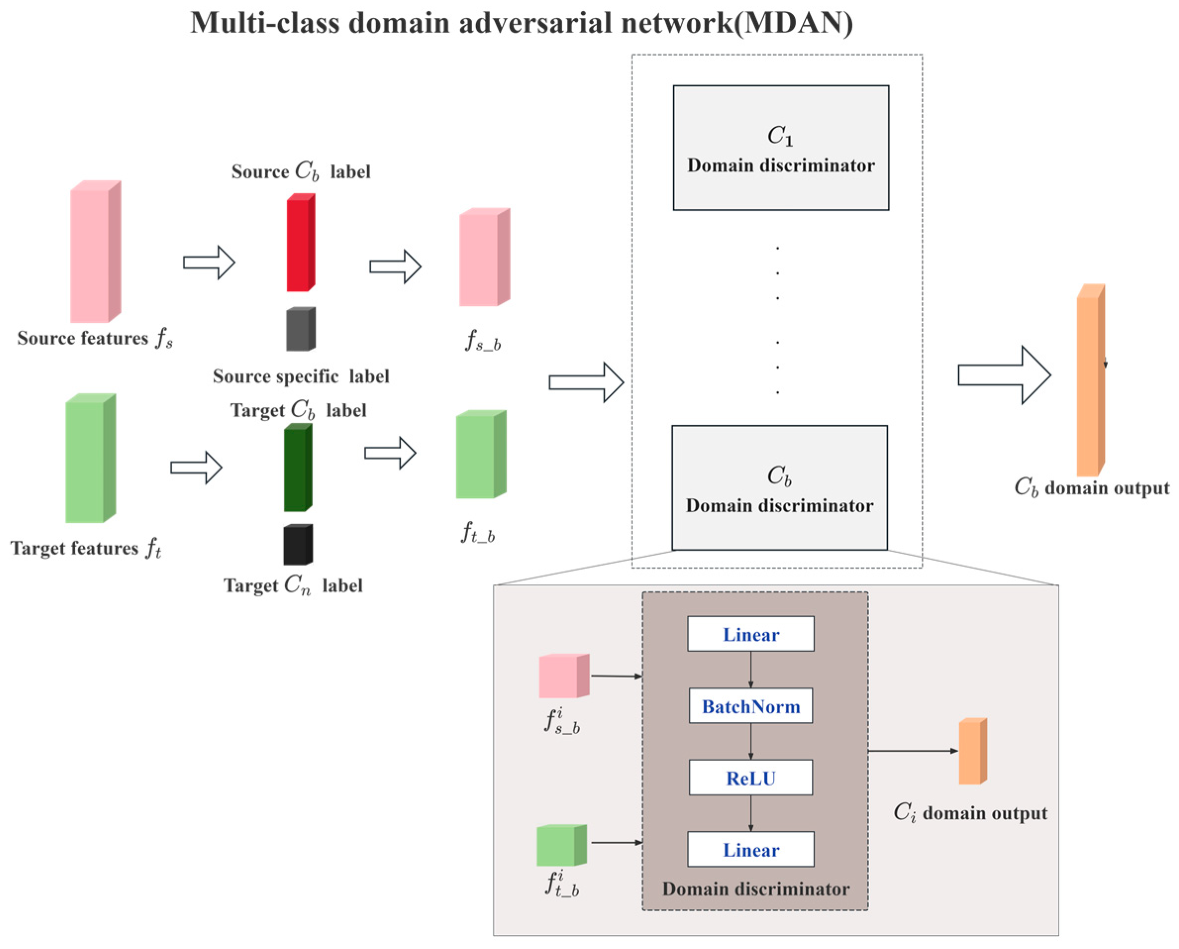
- A Multi-class Domain Adversarial Network (MDAN) was proposed to transfer the pre-trained feature extractor from source domain to target domain. By setting up independent discriminators for each base category, it promotes positive transfer of the base categories between source domain and target domain, avoiding negative transfer caused by unique categories.
- (3)
- An incremental learning strategy consisting of a Knowledge Transfer Module (KTM) and a Feature Separation Module (FSM) was designed to enable the model to segment novel categories while avoiding catastrophic base category data loss. For base categories, a Knowledge Transfer Module (KTM) consisting of Kullback–Leibler (KL) divergence and feature similarity was used to transfer knowledge. For novel categories, an FSM that utilized orthogonal loss functions as constraints was proposed to learn unique features for distinguishing base categories.
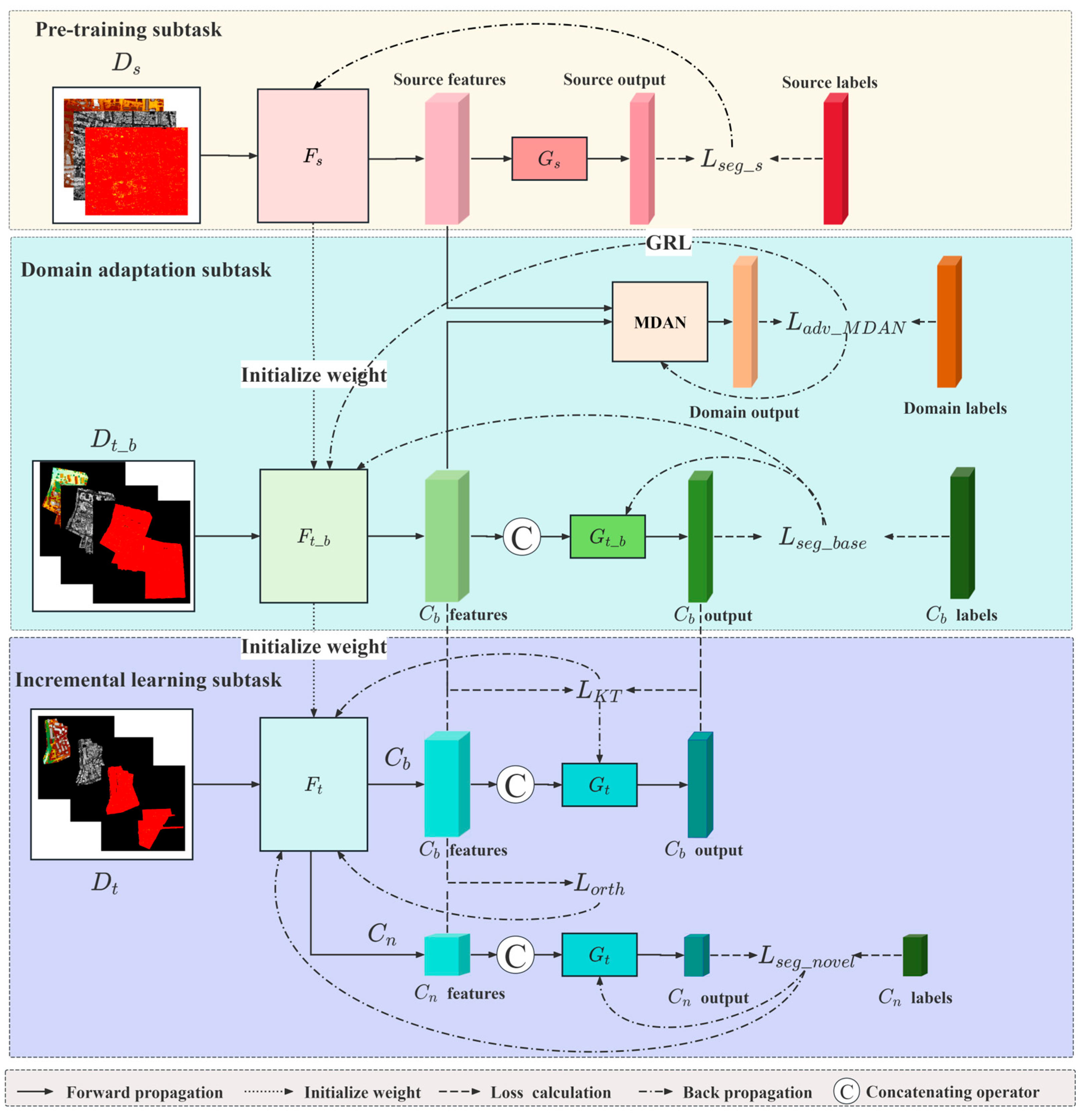
2. Method
2.1. Problem Definition
- (1)
- Pre-training subtask: Feature extractor was pre-trained in source domain .
- (2)
- Domain adaptation subtask: For the base categories , domain adaptation was employed to transfer the pre-trained adapted to the target domain as in the subdomain : , and target classifier was trained in the subdomain .
- (3)
- Incremental learning subtask: The feature extractor and classifier should be able to segment while retaining the ability to segment for in : , .
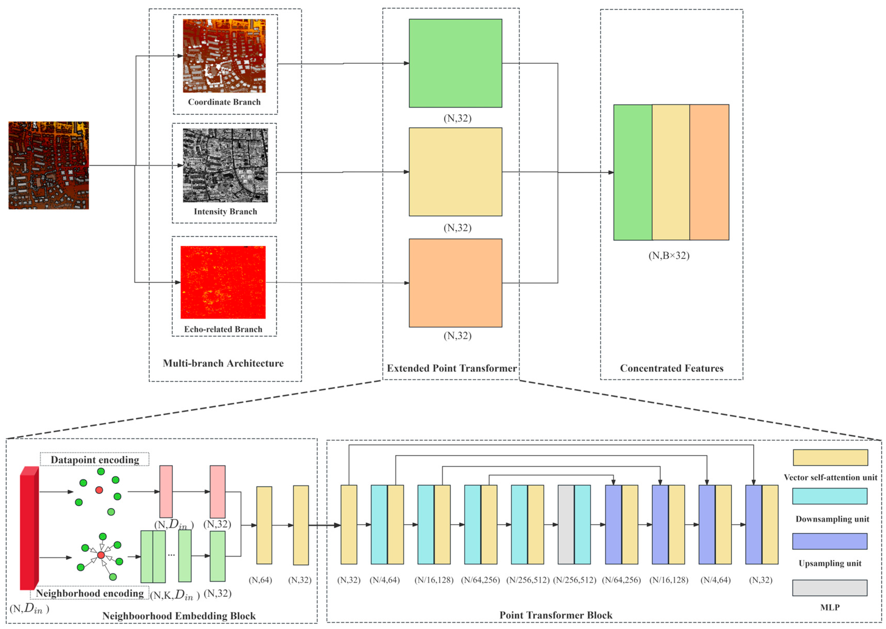
2.2. Multi-Branch Feature Extractor (MFE)
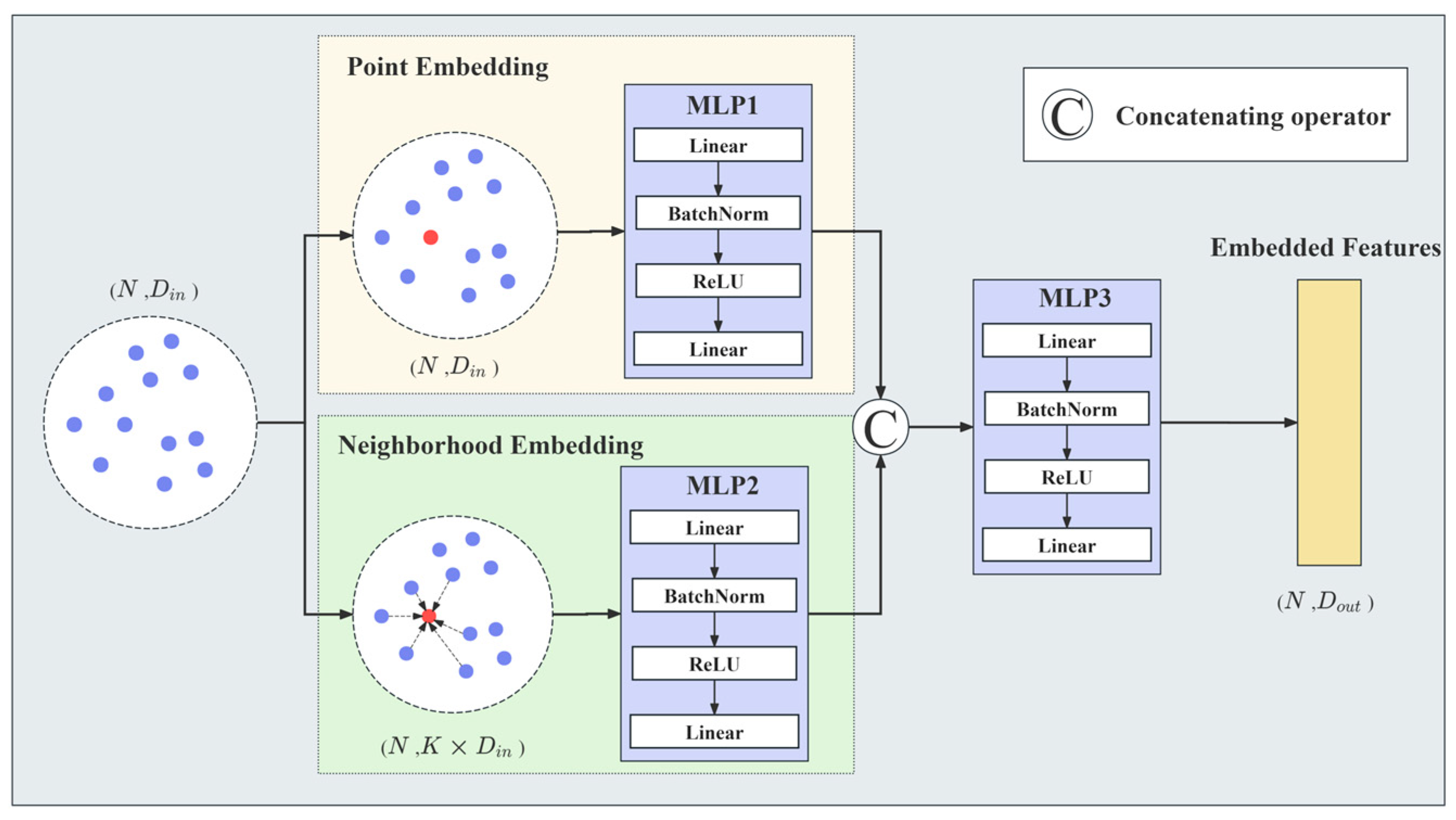
2.2.1. Neighborhood Embedding Block (NEB)
| Algorithm 1. Neighborhood Embedding Block |
| Input: ALS point cloud data , where N is the number of points, and is the dimension of the input. For instance, if the input is X, Y, and Z, then . Output: Embedded features , where is the dimension of the embedded features. Initialization: P is point sets, K is the number of neighboring points. 1: For in P: 2: Search for the K-nearest-neighboring points of the current point (); the points within the neighborhood are denoted by . 3: Obtain the original parameters of the current point () from point cloud data () as . 4: Encode the current point using MLP1: . 5: Encode the neighborhood of the current point using MLP2: . 6: Combine the encoded features to obtain the final features through MLP3: [ ]. 7: End for |
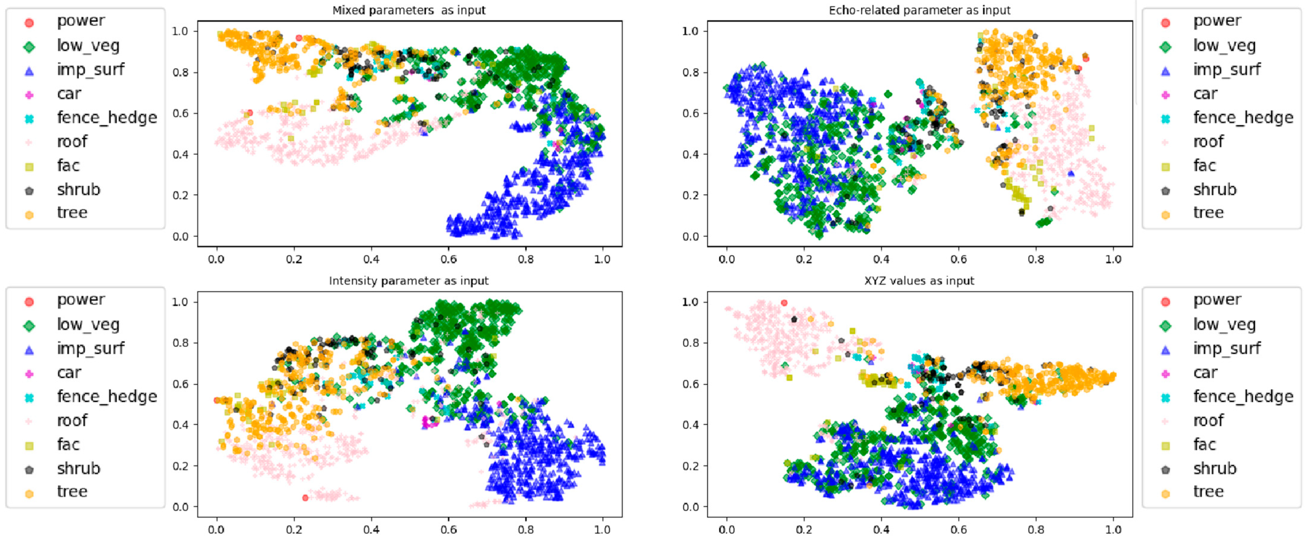
2.2.2. Concept of Multi-Branch Architecture
- (a)
- Mixed parameters (including XYZ values, intensity, and echo-related parameters), which are also commonly input into current deep learning methods for ALS point cloud analysis;
- (b)
- Echo-related parameters, which reflect the internal structure of ground objects;
- (c)
- Intensity, which characterizes the backscattering coefficient of ground objects;
- (d)
- XYZ values, which record the three-dimensional coordinate information of ground objects and are also the most commonly used parameters in traditional machine learning methods.
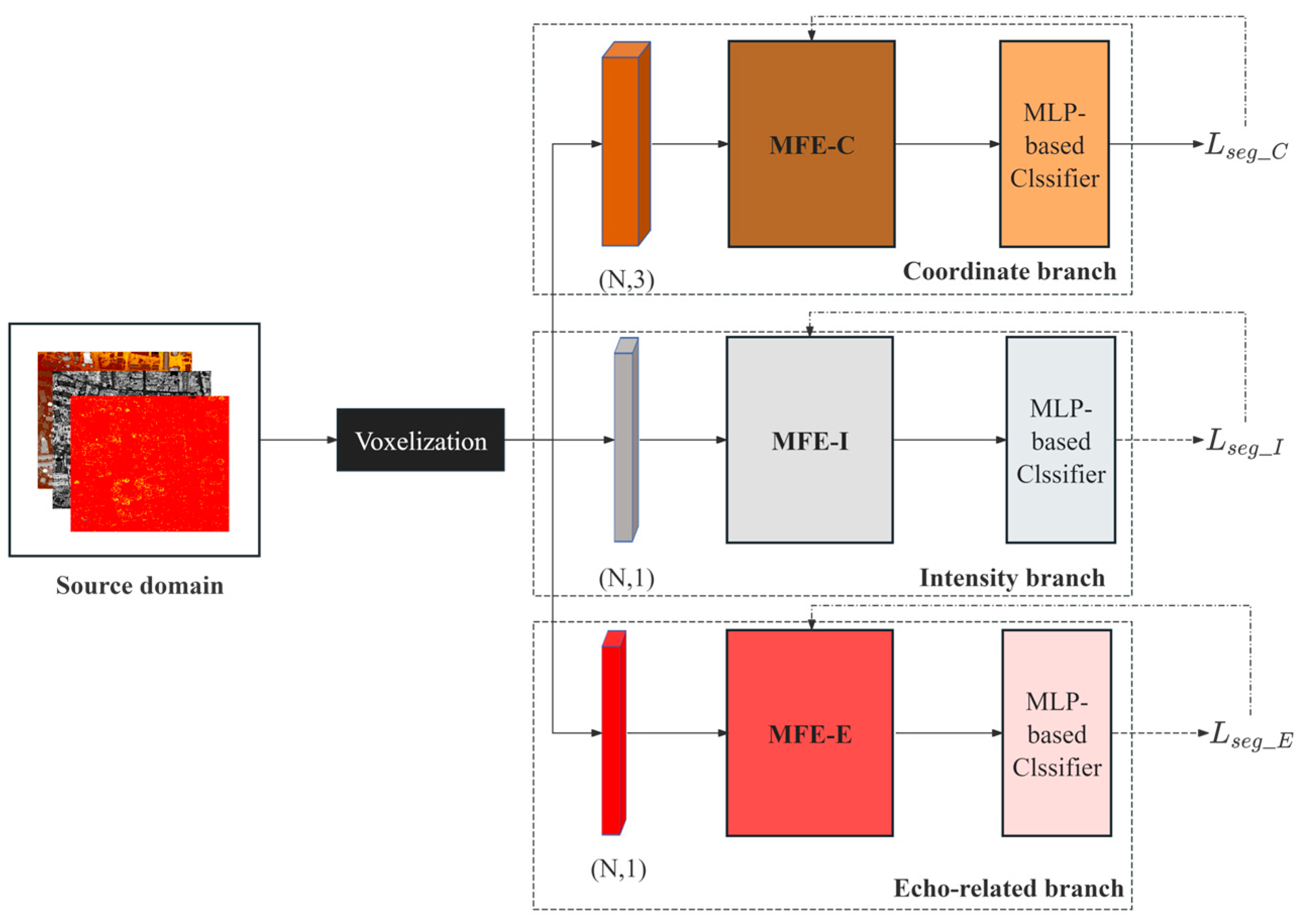
2.2.3. Construction of MFE Based on Multi-Branch Architecture
- (a)
- Coordinate branch: the input includes X, Y, and Z values. In the NEB, besides X, Y, and Z values, relative Z values of the K-nearest-neighboring points of the current point were input into the embedding features. Relative Z values were calculated because relative Z values are significant features to distinguish ground objects [40].
- (b)
- Intensity branch: The input is the intensity. In the NEB, the intensity of the current point and that of the K-nearest-neighboring points were input into the embedding features.
- (c)
- Echo-related branch: The input is the preprocessed echo-related parameters. In the NEB, echo-related parameters of the current point and those of the K-nearest-neighboring points were input into embedding features.
2.3. Pre-Training Subtask
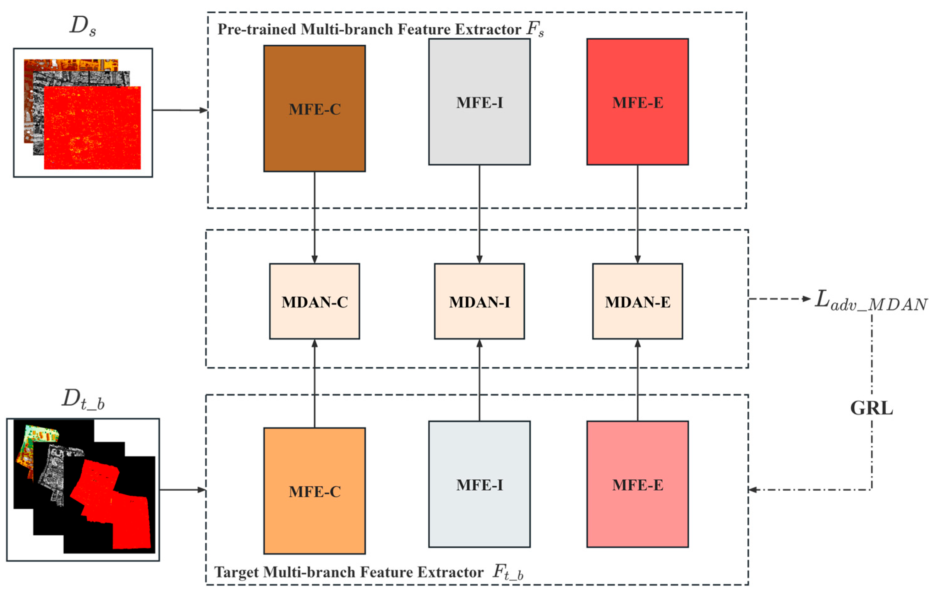
2.4. Domain Adaption Subtask
2.5. Incremental Learning Subtask
| Algorithm 2. Three-stage transfer learning strategy |
| Pre-training subtask |
| Input: Source domain , where is the number of total blocks after gridding the source domain. Output: Pre-trained consists of Multi-branch Feature Extractor and an MLP-based classification layer within each branch. The number of branches is set to 3, namely coordinate branch MFE-C, intensity branch MFE-I, and echo-related branch MFE-E. 1: For each block in : 2: Train -C, -I and -E using and calculate . 3: Backpropagate and update . 4: End for |
| Domain adaptation subtask |
| Input: Source domain and target domain with labeled base categories , where and are the number of blocks after gridding the source and target domain, respectively. Frozen pre-trained . MDAN consists of k MLP-based domain discriminators, where k is the number of base categories. Output: Domain-adapted consists of Multi-branch Feature Extractor and MLP-based classification layer . 1: For in [1, 2, 3, …,]: 2: Given a block from source domain and a block from target domain. 3: For each branch in {MFE-C, MFE-I, MFE-E}: 4: Features , are obtained by: , . 5: For each base category k: 6: Domain labels are obtained by : [, ] . 7: Loss is calculated. 8: End for 9: Loss is calculated by: . 10: End for 11: Train using and calculate the segmentation loss . 12: . 13: Backpropagate , updating and MDAN. 14: End for |
| Incremental learning subtask |
| Input: Target domain , where is the number of total blocks after gridding the target domain. Frozen domain adaptated . Output: consists of Multi-branch Feature Extractor and MLP-based classification layer . 1: For each block in : 2: For points with labeled base categories: 3: Features and logists are obtained by : . 4: Features and logists are obtained by : . 5: is calculated by and ; is calculated by and . 6: . 7: End for 8: For points with labeled novel categories: 9: Features are obtained by : . 10: Features and logists are obtained by : . 11: is calculated by and ; segmentation loss is calculated. 12: . 13: End for 14: 15: Backpropagate and update . 16: End for |
3. Experiments
3.1. Datasets and Evaluation Metrics
3.2. Experimental Results
3.2.1. Processing Details
- 1.
- Data preprocessing
- Coordinate values: Normalized after centralization, after which the range of value is 0~1.
- Intensity: Normalization, after which the range of value is 0~1.
- Echo-related parameters: Existing deep learning methods normalize the return number (RN) and number of returns (NR) separately [50]. Other studies pointed out that NR is positively correlated with the complexity of the internal structure [38]. Therefore, by combining RN and NR, a novel normalization method for echo-related parameters was proposed as follow:
- 2.
- Settings of pre-training subtask
- (1)
- Coordinate branch: Pre-trained using the DALES dataset and Dublin dataset.
- (2)
- Echo-related branch: Pre-trained using the DALES dataset and Dublin dataset.
- (3)
- Intensity branch: Pre-trained using the Dublin dataset.
- 3.
- Settings of domain adaptation subtask and incremental learning subtask
- 4.
- Other settings
3.2.2. Comparison of Experimental Results
- 1.
- Comparison with other fully supervised deep learning methods
- 2.
- Comparison with other few sample learning methods
4. Ablation Experiments and Discussions
4.1. Discussions of Neighborhood Embedding Block
4.2. Discussions of Multi-Branch Architecture
4.3. Discussion of Domain Adaptation Subtask and Incremental Learning Subtask
4.4. Analysis of the Impact of Random Sampling
5. Conclusions
Author Contributions
Funding
Data Availability Statement
Conflicts of Interest
References
- Liu, X.; Zhang, Z.; Peterson, J.; Chandra, S. Large area DEM generation using airborne LiDAR data and quality control. In Accuracy in Geomatics: Proceedings of the 8th International Symposium on Spatial Accuracy Assessment in Natural Resources and Environmental Sciences, Shanghai, China, 25–27 June 2008; World Academic Union: Liverpool, UK, 2008; Volume 2. [Google Scholar]
- Murakami, H.; Nakagawa, K.; Hasegawa, H.; Shibata, T.; Iwanami, E. Change detection of building using an airborne laser scanner. ISPRS J. Photogramm. Remote Sens. 1999, 54, 148–152. [Google Scholar] [CrossRef]
- Ivanovs, J.; Lazdins, A.; Lang, M. The influence of forest tree species composition on the forest height predicted from airborne laser scanning data—A case study in Latvia. Balt. For. 2023, 29, id663. [Google Scholar] [CrossRef]
- Matikainen, L.; Lehtomäki, M.; Ahokas, E.; Hyyppä, J.; Karjalainen, M.; Jaakkola, A.; Kukko, A.; Heinonen, T. Remote sensing methods for power line corridor surveys. ISPRS J. Photogramm. Remote Sens. 2016, 119, 10–31. [Google Scholar] [CrossRef]
- Guo, Y.; Wang, H.; Hu, Q.; Liu, H.; Liu, L.; Bennamoun, M. Deep learning for 3d point clouds: A survey. IEEE Trans. Pattern Anal. Mach. Intell. 2020, 43, 4338–4364. [Google Scholar] [CrossRef] [PubMed]
- An, Z.; Sun, G.; Liu, Y.; Liu, F.; Wu, Z.; Wang, D.; Van Gool, L.; Belongie, S. Rethinking few-shot 3d point cloud semantic segmentation. In Proceedings of the IEEE/CVF Conference on Computer Vision and Pattern Recognition, Seattle, WA, USA, 16–22 June 2024; pp. 3996–4006. [Google Scholar]
- Sarker, S.; Sarker, P.; Stone, G.; Gorman, R.; Tavakkoli, A.; Bebis, G.; Sattarvand, J. A comprehensive overview of deep learning techniques for 3D point cloud classification and semantic segmentation. Mach. Vis. Appl. 2024, 35, 67. [Google Scholar] [CrossRef]
- Huang, R.; Xu, Y.; Stilla, U. GraNet: Global relation-aware attentional network for semantic segmentation of ALS point cloud. ISPRS J. Photogramm. Remote Sens. 2021, 177, 1–20. [Google Scholar] [CrossRef]
- Liang, Z.; Lai, X. Multilevel geometric feature embedding in transformer network for ALS point cloud semantic segmentation. Remote Sens. 2024, 16, 3386. [Google Scholar] [CrossRef]
- Liu, T.; Wei, B.; Hao, J.; Li, Z.; Ye, F.; Wang, L. A multi-point focus transformer approach for large-scale ALS point cloud ground filtering. Int. J. Remote Sens. 2025, 46, 979–999. [Google Scholar] [CrossRef]
- Zhao, J.; Zhou, H. Cross-layer Features Fusion Network with Attention MLP for ALS Point Cloud Segmentation. In Proceedings of the 5th International Conference on Computer Vision, Zhuhai, China, 19–21 April 2024; Image and Deep Learning (CVIDL). IEEE: New York, NY, USA, 2024; pp. 1110–1114. [Google Scholar]
- Hu, Q.; Yang, B.; Xie, L.; Rosa, S.; Guo, Y.; Wang, Z.; Trigoni, N.; Markham, A. Randla-net: Efficient semantic segmentation of large-scale point cloud. In Proceedings of the IEEE/CVF Conference on Computer Vision and Pattern Recognition, Seattle, WA, USA, 13–19 June 2020; pp. 11108–11117. [Google Scholar]
- Qi, C.R.; Su, H.; Mo, K.; Guibas, L.J. Pointnet: Deep learning on point sets for 3d classification and segmentation. In Proceedings of the IEEE Conference on Computer Vision and Pattern Recognition, Honolulu, HI, USA, 21–26 July 2017; pp. 652–660. [Google Scholar]
- Qi, C.R.; Yi, L.; Su, H.; Guibas, L.J. Pointnet++: Deep hierarchical feature learning on point sets in a metric space. Adv. Neural Inf. Process Syst. 2017, 30, 5105–5114. [Google Scholar]
- Phan, A.V.; Le Nguyen, M.; Nguyen, Y.L.H.; Bui, L.T. Dgcnn: A convolutional neural network over large-scale labeled graphs. Neural Netw. 2018, 108, 533–543. [Google Scholar] [CrossRef]
- Zhou, Y.; Tuzel, O. Voxelnet: End-to-end learning for point cloud based 3d object detection. In Proceedings of the IEEE Conference on Computer Vision and Pattern Recognition, Salt Lake City, UT, USA, 18–23 June 2018; pp. 4490–4499. [Google Scholar]
- Wang, Y.; Sun, Y.; Liu, Z.; Sarma, S.E.; Bronstein, M.M.; Solomon, J.M. Dynamic graph cnn for learning on point cloud. ACM Trans. Graph. (TOG) 2019, 38, 1–12. [Google Scholar] [CrossRef]
- Zhao, H.; Jiang, L.; Jia, J.; Torr, P.H.; Koltun, V. Point transformer. In Proceedings of the IEEE/CVF International Conference on Computer Vision, Montreal, QC, Canada, 10–17 October 2021; pp. 16259–16268. [Google Scholar]
- Park, C.; Jeong, Y.; Cho, M.; Park, J. Fast point transformer. In Proceedings of the IEEE/CVF Conference on Computer Vision and Pattern Recognition, New Orleans, LA, USA, 18–24 June 2022; pp. 16949–16958. [Google Scholar]
- Wang, P.S. Octformer: Octree-based transformers for 3d point clouds. ACM Trans. Graph. (TOG) 2023, 42, 1–11. [Google Scholar] [CrossRef]
- Guo, M.H.; Cai, J.X.; Liu, Z.N.; Mu, T.J.; Martin, R.R.; Hu, S.M. Pct: Point cloud transformer. Comput. Vis. Media 2021, 7, 187–199. [Google Scholar] [CrossRef]
- Kheddar, H.; Himeur, Y.; Al-Maadeed, S.; Amira, A.; Bensaali, F. Deep transfer learning for automatic speech recognition: Towards better generalization. Knowl.-Based Syst. 2023, 277, 110851. [Google Scholar] [CrossRef]
- Bozinovski, S. Reminder of the first paper on transfer learning in neural networks, 1976. Informatica 2020, 44, 291. [Google Scholar] [CrossRef]
- Iman, M.; Arabnia, H.R.; Rasheed, K. A review of deep transfer learning and recent advancements. Technologies 2023, 11, 40. [Google Scholar] [CrossRef]
- Niu, S.; Liu, Y.; Wang, J.; Song, H. A decade survey of transfer learning (2010–2020). IEEE Trans. Artif. Intell. 2021, 1, 151–166. [Google Scholar] [CrossRef]
- Ma, H.; Cai, Z.; Zhang, L. Comparison of the filtering models for airborne LiDAR data by three classifiers with exploration on model transfer. J. Appl. Remote Sens. 2018, 12, 016021. [Google Scholar] [CrossRef]
- Ahmed, S.F.; Alam, M.S.B.; Hassan, M.; Rozbu, M.R.; Ishtiak, T.; Rafa, N.; Mofijur, M.; Shawkat Ali, A.; Gandomi, A. Deep learning modelling techniques: Current progress, applications, advantages, and challenges. Artif. Intell. Rev. 2023, 56, 13521–13617. [Google Scholar] [CrossRef]
- Peng, S.; Xi, X.; Wang, C.; Xie, R.; Wang, P.; Tan, H. Point-based multilevel domain adaptation for point cloud segmentation. IEEE Geosci. Remote Sens. Lett. 2020, 19, 1–5. [Google Scholar] [CrossRef]
- Xie, Y.; Schindler, K.; Tian, J.; Zhu, X.X. Exploring cross-city semantic segmentation of ALS point clouds. Int. Arch. Photogramm. Remote Sens. Spat. Inf. Sci. 2021, 43, 247–254. [Google Scholar] [CrossRef]
- Zhao, C.; Yu, D.; Xu, J.; Zhang, B.; Li, D. Airborne LiDAR point cloud classification based on transfer learning. In Proceedings of the Eleventh International Conference on Digital Image Processing (ICDIP 2019), Guangzhou, China, 10–13 May 2019; SPIE: Bellingham, WA, USA, 2019; Volume 11179, pp. 550–556. [Google Scholar]
- Dai, M.; Xing, S.; Xu, Q.; Li, P.; Pan, J.; Zhang, G.; Wang, H. Multiprototype Relational Network for Few-Shot ALS Point Cloud Semantic Segmentation by Transferring Knowledge From Photogrammetric Point Clouds. IEEE Trans. Geosci. Remote Sens. 2024, 62, 1–17. [Google Scholar] [CrossRef]
- Dai, M.; Xing, S.; Xu, Q.; Li, P.; Pan, J.; Wang, H. Cross-Domain Incremental Feature Learning for ALS Point Cloud Semantic Segmentation with Few Samples. IEEE Trans. Geosci. Remote Sens. 2024, 63, 1–14. [Google Scholar] [CrossRef]
- Long, M.; Cao, Z.; Wang, J.; Jordan, M.I. Conditional Adversarial Domain Adaptation. In Proceedings of the Computer Vision—ECCV 2018—15th European Conference, Munich, Germany, 8–14 September 2018; Springer: Cham, Switzerland, 2018. [Google Scholar] [CrossRef]
- Tzeng, E.; Hoffman, J.; Saenko, K.; Darrell, T. Adversarial Discriminative Domain Adaptation. arXiv 2017. [Google Scholar] [CrossRef]
- Kirkpatrick, J.; Pascanu, R.; Rabinowitz, N.; Veness, J.; Desjardins, G.; Rusu, A.A.; Milan, K.; Quan, J.; Ramalho, T.; Grabska-Barwinska, A. Overcoming catastrophic forgetting in neural networks. Proc. Natl. Acad. Sci. USA 2017, 114, 3521–3526. [Google Scholar] [CrossRef]
- Neyshabur, B.; Sedghi, H.; Zhang, C. What is being transferred in transfer learning? Adv. Neural Inf. Process. Syst. 2020, 33, 512–523. [Google Scholar]
- Ni, H.; Lin, X.; Zhang, J. Classification of ALS point cloud with improved point cloud segmentation and random forests. Remote Sens. 2017, 9, 288. [Google Scholar] [CrossRef]
- Reymann, C.; Lacroix, S. Improving LiDAR point cloud classification using intensities and multiple echoes. In Proceedings of the 2015 IEEE/RSJ International Conference on Intelligent Robots and Systems (IROS), Hamburg, Germany, 28 September–3 October 2015; IEEE: New York, NY, USA, 2015; pp. 5122–5128. [Google Scholar]
- Stanislas, L.; Nubert, J.; Dugas, D.; Nitsch, J.; Sünderhauf, N.; Siegwart, R.; Cadena, C.; Peynot, T. Airborne particle classification in lidar point clouds using deep learning. In Field and Service Robotics: Results of the 12th International Conference; Springer: Singapore, 2021; pp. 395–410. [Google Scholar]
- Zhang, K.; Ye, L.; Xiao, W.; Sheng, Y.; Zhang, S.; Tao, X.; Zhou, Y. A dual attention neural network for airborne LiDAR point cloud semantic segmentation. IEEE Trans. Geosci. Remote Sens. 2022, 60, 1–17. [Google Scholar] [CrossRef]
- Mahajan, D.; Girshick, R.; Ramanathan, V.; He, K.; Paluri, M.; Li, Y.; Bharambe, A.; Van Der Maaten, L. Exploring the limits of weakly supervised pretraining. In Proceedings of the European conference on computer vision (ECCV), Munich, Germany, 8–14 September 2018; pp. 181–196. [Google Scholar]
- Panigrahi, S.; Nanda, A.; Swarnkar, T. A survey on transfer learning. In Intelligent and Cloud Computing: Proceedings of ICICC 2019, Bhubaneswar, India, 20 December 2019; Springer: Singapore, 2020; Volume 1, pp. 781–789. [Google Scholar]
- Ganin, Y.; Ustinova, E.; Ajakan, H.; Germain, P.; Larochelle, H.; Laviolette, F.; March, M.; Lempitsky, V. Domain-Adversarial Training of Neural Networks. J. Mach. Learn. Res. 2016, 17, 1–35. [Google Scholar] [CrossRef]
- Pei, Z.; Cao, Z.; Long, M.; Wang, J. Multi-Adversarial Domain Adaptation. In Proceedings of the AAAI conference on artificial intelligence, New Orleans, LA, USA, 2–7 February 2018; AAAI Press: Palo Alto, CA, USA, 2018. [Google Scholar] [CrossRef]
- Yu, Z.; Wang, K.; Xie, S.; Zhong, Y.; Lv, Z. Prototypical Network Based on Manhattan Distance. CMES-Comput. Model. Eng. Sci. 2022, 131, 655. [Google Scholar] [CrossRef]
- Cramer, M. The dgpf-test on digital airborne camera evaluation–overview and test design. Photogramm.-Fernerkund.-Geoinf. 2010, 73–82. [Google Scholar] [CrossRef]
- Rottensteiner, F.; Sohn, G.; Jung, J.; Gerke, M.; Baillard, C.; Benitez, S.; Breitkopf, U. The isprs benchmark on urban object classification and 3D building reconstruction. ISPRS Ann. Photogramm. Remote Sens. Spat. Inf. Sci. 2012, 1–3, 293–298. [Google Scholar] [CrossRef]
- Iman Zolanvari, S.M.; Ruano, S.; Rana, A.; Cummins, A.; da Silva, R.E.; Rahbar, M.; Smolic, A. Dublin City: Annotated LiDAR Point Cloud and its Applications. arXiv 2019. [Google Scholar] [CrossRef]
- Varney, N.; Asari, V.K.; Graehling, Q. DALES: A Large-scale Aerial LiDAR Data Set for Semantic Segmentation. In Proceedings of the IEEE/CVF Conference on Computer Vision and Pattern Recognition Workshops (CVPRW), Seattle, WA, USA, 14–19 June 2020; IEEE: New York, NY, USA, 2020. [Google Scholar] [CrossRef]
- Wang, J.; Li, H.; Xu, Z.; Xie, X. Semantic segmentation of urban airborne LiDAR point clouds based on fusion attention mechanism and multi-scale features. Remote Sens. 2023, 15, 5248. [Google Scholar] [CrossRef]
- Thomas, H.; Qi, C.R.; Deschaud, J.E.; Marcotegui, B.; Goulette, F.; Guibas, L.J. KPConv: Flexible and Deformable Convolution for Point Clouds. In Proceedings of the 2019 IEEE/CVF International Conference on Computer Vision (ICCV), Seoul, Republic of Korea, 27 October–2 November 2019; IEEE: New York, NY, USA, 2020. [Google Scholar] [CrossRef]
- Li, X.; Wang, L.; Wang, M.; Wen, C.; Fang, Y. Dance-net: Density-aware convolution networks with context encoding for airborne lidar point cloud classification. ISPRS J. Photogramm. Remote Sens. 2020, 166, 128–139. [Google Scholar] [CrossRef]
- Li, W.; Wang, F.-D.; Xia, G.-S. A geometry-attentional network for ALS point cloud classification. ISPRS J. Photogramm. Remote Sens. 2020, 164, 26–40. [Google Scholar] [CrossRef]
- Mao, Y.; Chen, K.; Diao, W.; Sun, X.; Lu, X.; Fu, K.; Weinmann, M. Beyond single receptive field: A receptive field fusion-and-stratification network for airborne laser scanning point cloud classification. ISPRS J. Photogramm. Remote Sens. 2022, 188, 45–61. [Google Scholar] [CrossRef]
- Chen, Y.; Xing, Y.; Li, X.; Gao, W. DGCN-ED: Dynamic graph convolutional networks with encoder–decoder structure and its application for airborne LiDAR point classification. Int. J. Remote Sens. 2023, 44, 3489–3506. [Google Scholar] [CrossRef]
- Mao, Y.Q.; Bi, H.; Li, X.; Chen, K.; Wang, Z.; Sun, X.; Fu, K. Twin deformable point convolutions for airborne laser scanning point cloud classification. ISPRS J. Photogramm. Remote Sens. 2025, 221, 78–91. [Google Scholar] [CrossRef]
- Wang, Z.; Chen, H.; Liu, J.; Qin, J.; Sheng, Y.; Yang, L. Multilevel intuitive attention neural network for airborne LiDAR point cloud semantic segmentation. Int. J. Appl. Earth Obs. Geoinf. 2024, 132, 104020. [Google Scholar] [CrossRef]
- Hu, Q.; Yang, B.; Khalid, S.; Xiao, W.; Trigoni, N.; Markham, A. Towards Semantic Segmentation of Urban-Scale 3D Point Clouds: A Dataset, Benchmarks and Challenges (CVPR’2021). In Proceedings of the IEEE/CVF Conference on Computer Vision and Pattern Recognition, Seattle, WA, USA, 13–19 June 2020. [Google Scholar]


| Methods | Brief Descriptions | Advantages and Limitations |
|---|---|---|
| MLP-based methods [12,13,14] | A shared multi-layer perceptron (MLP) is adopted as the core building block. Aggregating features are complemented by symmetric functions. | Simple and efficient, but underperforms when the point cloud contains complex local structures. |
| Convolution-based methods [15,16,17] | Inspired by the success of convolution kernels in image segmentation, they are adopted for point clouds in order to extract local geometries. | Mature deep learning models can be adopted, but this type of method requires converting the point cloud into a 2D/3D regular structure first by gridding/voxelization, and information loss is unavoidable during this process. Moreover, the input order of the point cloud may cause differences in the segmentation results. |
| Attention-based methods [18,19,20,21] | Long-range dependencies are modeled by attention mechanisms, which are suitable for handling point cloud irregularities. | Attention-based methods have achieved superior results, but this type of method has a high demand for computing resources, and a large amount of high-quality annotated data is required to ensure its high performance. |
| Domain | Target Domain | Source Domain | |
|---|---|---|---|
| Dataset | ISPRS benchmark dataset | DALES dataset | Dublin dataset |
| Density | Above 4 pts/m2 | Above 50 pts/m2 | >150 pts/m2 |
| Parameter type | XYZ values Intensity Echo-related parameters | XYZ values Echo-related parameters | XYZ Values intensity Echo-related parameters |
| Categories | Powerlines, low_veg, imp_sur (ground), cars, fence/hedge (fences), roof (building), fac, shrub, tree (vegetation) | Ground, vegetation, cars, trucks, powerlines, poles, fences, building | Building, ground and vegetation |
| Base categories | Ground, vegetation, car, building, fence, powerlines | ||
| Novel categories | low_veg, fac, shrub | - | - |
| Proportion | Base Categories | Novel Categories | |||||||
|---|---|---|---|---|---|---|---|---|---|
| Power | Imp_Surf | Car | Fence | Roof | Tree | Low_Veg | Fac | Shrub | |
| 100% | 546 | 193,723 | 4614 | 12,070 | 152,045 | 135,173 | 180,580 | 27,250 | 47,605 |
| 10% | 55 | 19,383 | 462 | 1207 | 15,205 | 13,518 | 18,058 | 2725 | 4761 |
| 1% | 6 | 1939 | 47 | 121 | 1521 | 1352 | 1806 | 273 | 477 |
| 0.1% | 1 | 194 | 5 | 13 | 153 | 136 | 181 | 28 | 48 |
| Method | Power | Low_Veg | Imp_Surf | Car | Fence | Roof | Fac | Shrub | Tree | OA | averF1 |
|---|---|---|---|---|---|---|---|---|---|---|---|
| PointNet++ (2017) [14] | 57.9 | 79.6 | 90.6 | 66.1 | 31.5 | 91.6 | 54.3 | 41.6 | 77.0 | 81.2 | 65.6 |
| KPConv (2019) [51] | 63.1 | 82.3 | 91.4 | 72.5 | 25.2 | 94.4 | 60.3 | 44.9 | 81.2 | 83.7 | 68.4 |
| DANCE-NET (2020) [52] | 68.4 | 81.6 | 92.8 | 77.2 | 38.6 | 93.9 | 60.2 | 47.2 | 81.4 | 83.9 | 71.2 |
| GANet (2020) [53] | 75.4 | 82.0 | 91.6 | 77.8 | 44.2 | 94.4 | 61.5 | 49.6 | 82.6 | 84.5 | 73.2 |
| GraNet (2021) [18] | 67.7 | 82.7 | 91.7 | 80.9 | 51.1 | 94.5 | 62.0 | 49.9 | 82.0 | 84.5 | 73.6 |
| RFFS-NET (2022) [54] | 75.5 | 80.0 | 90.5 | 78.5 | 45.5 | 92.7 | 57.9 | 48.3 | 75.7 | 82.1 | 71.6 |
| DGCN-ED (2023) [55] | 72.6 | 82.9 | 92.3 | 75.9 | 41.8 | 92.1 | 60.9 | 43.4 | 79.5 | 83.5 | 71.3 |
| TDConvs (2024) [56] | 67.0 | 82.4 | 91.6 | 84.7 | 48.7 | 94.2 | 63.3 | 46.9 | 81.7 | 84.5 | 73.4 |
| MIA-Net (2024) [57] | 65.8 | 79.5 | 89.7 | 71.1 | 26.2 | 94.0 | 63.5 | 48.1 | 82.8 | 83.3 | 71.8 |
| Ours (10%) | 72.9 | 83.1 | 91.9 | 83.4 | 42.1 | 95.4 | 63.9 | 51.7 | 82.8 | 85.5 | 74.0 |
| Ours (1%) | 65.2 | 81.6 | 90.3 | 66.1 | 31.6 | 94.1 | 60.1 | 43.5 | 82.6 | 83.7 | 68.4 |
| Ours (0.1%) | 59.6 | 80.2 | 89.7 | 62.9 | 26.1 | 92.5 | 58.3 | 36.1 | 80.7 | 81.8 | 65.1 |
| Ours (100%) | 76.3 | 83.4 | 91.8 | 83.2 | 37.6 | 95.5 | 68.4 | 52.8 | 83.9 | 85.7 | 74.7 |
| Domain | Target Domain | Source Domain | |
|---|---|---|---|
| Dataset | ISPRS benchmark dataset | SensatUrban | |
| Parameter type | XYZ values Intensity Echo-related parameters | XYZ values RGB | |
| Number of categories | 9 | 12 | |
| Base categories | Ground, vegetation, building | ||
| Novel categories | Power, low_veg, car, fence, fac, shrub | — | |
| Settings of Multi-branch Feature Extractor | Components | (1) Coordinate branch, (2) intensity branch, (3) echo-related branch | |
| Pre-training subtask | _ | Coordinate branch: pre-training using XYZ values of SensatUrban dataset | |
| Domain adaptation subtask | (1) Coordinate branch: domain adaptation using sampled training set with base categories (2) Intensity branch and echo-related branch: supervised learning using sampled training set with base categories | - | |
| Incremental learning subtask | Coordinate branch, intensity branch, and echo-related branch: incremental learning using sampled training set with base categories and novel categories | - | |
| Method | Power | Low_Veg | Imp_Surf | Car | Fence | Roof | Fac | Shrub | Tree | OA | mIoU |
|---|---|---|---|---|---|---|---|---|---|---|---|
| Thr-MPRNet (2024) [37] | 0.0 | 60.58 | 70.6 | 8.6 | 1.7 | 57.8 | 12.08 | 17.4 | 44.7 | 44.1 | 32.4 |
| Dai (2025) [32] | 0.0 | 43.9 | 84.0 | 12.0 | 1.5 | 47.2 | 15.6 | 18.2 | 59.6 | 48.1 | 37.3 |
| Ours | 51.8 | 70.3 | 84.6 | 58.8 | 27.7 | 89.1 | 44.3 | 28.0 | 67.9 | 84.2 | 58.1 |
| Method | OA | p-Values (OA) | averF1 | p-Value (averF1) |
|---|---|---|---|---|
| Base | 80.1 (±0.18) | - | 62.9 (±0.74) | - |
| NEB (K = 4) | 80.9 (±0.26) | 0.009 | 65.6 (±0.72) | <0.0001 |
| NEB (K = 8) | 81.2 (±0.24) | 0.0005 | 66.7 (±0.83) | 0.001 |
| NEB (K = 16) | 81.8 (±0.28) | 0.0008 | 67.1 (±0.76) | 0.0006 |
| NEB (K = 32) | 81.7 (±0.21) | 0.0006 | 66.53 (±0.77) | 0.005 |
| NEB (K = 64) | 80.5 (±0.22) | 0.04 | 63.2 (±0.72) | 0.49 |
| Model | Description |
|---|---|
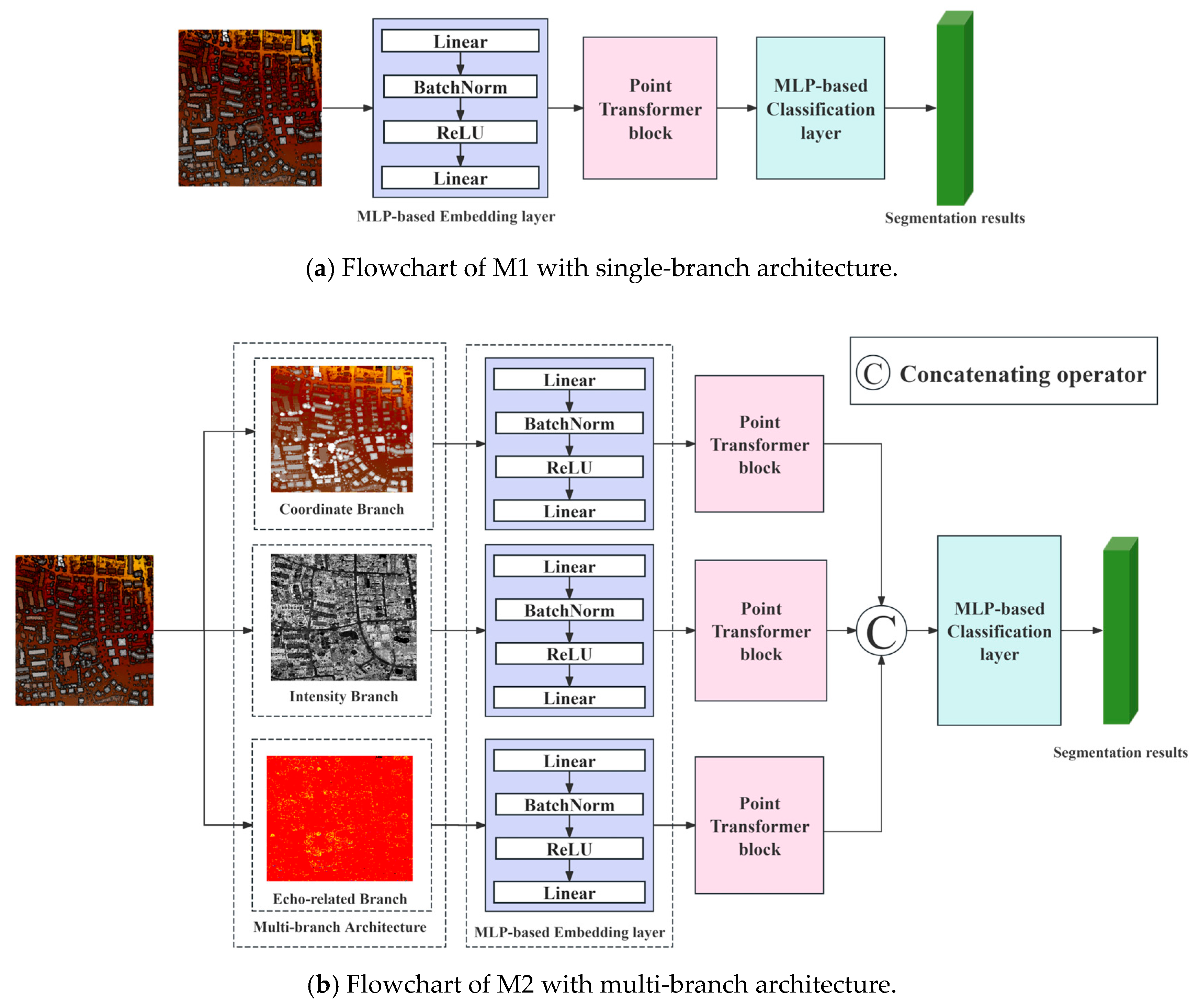
| M1 | Model consists of an MLP-based embedding layer, Point Transformer Block (PTB), and MLP-based classifier. The input data is a 5-dimensional vector that includes 3 coordinate values, intensity, and an echo-related parameter. |
| M2 | Model consists of a three-branch feature extractor that includes a coordinate branch, an intensity branch, and an echo-related branch. Each branch consists of an MLP-based embedding layer and PTB. Features from each branch were concatenated and then input into an MLP-based classifier to obtain segmentation results. |
| Method | Power | Low_Veg | Imp_Surf | Car | Fence | Roof | Fac | Shrub | Tree | OA | averF1 | p-Value (OA) | p-Value (averF1) |
|---|---|---|---|---|---|---|---|---|---|---|---|---|---|
| M1 | 50.2 (±5.41) | 80.4 (±0.28) | 91.0 (±0.25) | 67.4 (±1.94) | 21.6 (±5.15) | 92.8 (±0.25) | 56.7 (±0.48) | 46.7 (±0.43) | 80.5 (±0.28) | 82.4 (±0.28) | 65.3 (±0.82) | - | - |
| M2 | 67.1 (±4.82) | 82.3 (±0.34) | 91.2 (±0.23) | 70.5 (±2.17) | 33.6 (±3.24) | 94.5 (±0.21) | 60.7 (±0.52) | 49.3 (±0.38) | 80.8 (±0.31) | 83.7 (±0.26) | 69.8 (±0.78) | 0.0008 | 0.0007 |
| Method | Maximum (Second) | Minimum (Second) | Average (Second) |
|---|---|---|---|
| M1 | 28.7 | 31.9 | 30.7 |
| M2 | 55.3 | 61.4 | 58.6 |
| Method | Power | Imp_Surf | Car | Fence | Roof | Tree | OA | p-Value (OA) |
|---|---|---|---|---|---|---|---|---|
| FT | 50.4 (±5.89) | 97.9 (±0.14) | 66.3 (±1.91) | 48.9 (±5.41) | 90.7 (±0.21) | 84.1 (±0.25) | 90.3 (±0.28) | <0.0001 |
| MADA | 57.1 (±4.76) | 98.3 (±0.17) | 78.6 (±2.41) | 55.2 (±4.68) | 97.5 (±0.12) | 93.7 (±0.18) | 95.8 (±0.24) | <0.0001 |
| MDAN (Ours) | 76.9 (±3.46) | 98.5 (±0.11) | 82.6 (±1.81) | 61.4 (±4.32) | 98.0 (±0.15) | 93.9 (±0.2) | 96.5 (±0.17) | - |
| Method | OA | p-Value (OA) | |||||
|---|---|---|---|---|---|---|---|
| OA | Low_Veg | Fac | Shrub | OA | |||
| Base | 96.5 | - | - | - | - | - | - |
| KTM + Fine-tuning | 91.7 (±0.25) | 74.5 (±0.37) | 42.8 (±0.92) | 41.6 (±1.27) | 62.7 (±0.45) | 82.2 (±0.34) | <0.0001 |
| FSM | 81.0 (±0.19) | 84.0 (±0.28) | 69.5 (±0.86) | 65.1 (±0.93) | 78.1 (±0.38) | 80.1 (±0.23) | 0.0001 |
| Ours (KTM + FSM) | 91.7 (±0.25) | 83.2 (±0.19) | 64.2 (±0.73) | 52.1 (±0.84) | 73.2 (±0.26) | 85.5 (±0.25) | - |
| Method | |||||
|---|---|---|---|---|---|
| Low_Veg | Fac | Shrub | OA | p-Value (OA) | |
| SALM | 80.4 (±0.81) | 58.3 (±1.45) | 56.8 (±0.96) | 77.1 (±0.9) | - |
| FSM | 84.0 (±0.28) | 69.5 (±0.86) | 65.1 (±0.93) | 78.1 (±0.38) | 0.008 |
| Proportion | Maximum | Minimum | Average | |
|---|---|---|---|---|
| 10% | OA | 85.7 | 85.2 | 85.5 |
| averF1 | 74.3 | 72.1 | 73.8 | |
| 1% | OA | 84.1 | 83.4 | 83.8 |
| averF1 | 67.1 | 69.2 | 68.4 | |
| 0.1% | OA | 81.9 | 80.7 | 81.6 |
| averF1 | 65.6 | 62.1 | 64.1 | |
Disclaimer/Publisher’s Note: The statements, opinions and data contained in all publications are solely those of the individual author(s) and contributor(s) and not of MDPI and/or the editor(s). MDPI and/or the editor(s) disclaim responsibility for any injury to people or property resulting from any ideas, methods, instructions or products referred to in the content. |
© 2025 by the authors. Licensee MDPI, Basel, Switzerland. This article is an open access article distributed under the terms and conditions of the Creative Commons Attribution (CC BY) license (https://creativecommons.org/licenses/by/4.0/).
Share and Cite
Yuan, J.; Ma, H.; Zhang, L.; Deng, J.; Luo, W.; Liu, K.; Cai, Z. Transfer Learning Based on Multi-Branch Architecture Feature Extractor for Airborne LiDAR Point Cloud Semantic Segmentation with Few Samples. Remote Sens. 2025, 17, 2618. https://doi.org/10.3390/rs17152618
Yuan J, Ma H, Zhang L, Deng J, Luo W, Liu K, Cai Z. Transfer Learning Based on Multi-Branch Architecture Feature Extractor for Airborne LiDAR Point Cloud Semantic Segmentation with Few Samples. Remote Sensing. 2025; 17(15):2618. https://doi.org/10.3390/rs17152618
Chicago/Turabian StyleYuan, Jialin, Hongchao Ma, Liang Zhang, Jiwei Deng, Wenjun Luo, Ke Liu, and Zhan Cai. 2025. "Transfer Learning Based on Multi-Branch Architecture Feature Extractor for Airborne LiDAR Point Cloud Semantic Segmentation with Few Samples" Remote Sensing 17, no. 15: 2618. https://doi.org/10.3390/rs17152618
APA StyleYuan, J., Ma, H., Zhang, L., Deng, J., Luo, W., Liu, K., & Cai, Z. (2025). Transfer Learning Based on Multi-Branch Architecture Feature Extractor for Airborne LiDAR Point Cloud Semantic Segmentation with Few Samples. Remote Sensing, 17(15), 2618. https://doi.org/10.3390/rs17152618