Estimation of Footprint-Scale Across-Track Slopes Based on Elevation Frequency Histogram from Single-Track ICESat-2 Photon Data of Strong Beam

Abstract

Topographic slope is a key parameter for characterizing landscape geomorphology. The Ice, Cloud, and Land Elevation Satellite-2 (ICESat-2) offers high-resolution along-track slopes based on the ground profiles generated by dense signal photons. However, the across-track slopes are typically derived using the ground photon geolocations from the weak-beam and strong-beam pair, limiting the retrieval accuracy and losing valid results over rugged terrains. The goal of this study is to propose a new method to derive the across-track slope merely using single-track photon data of a strong beam based on the theoretical formula of the received signal pulse width. Based on the ICESat-2 photon data over the Walker Lake area, the specific purposes are to (1) extract the along-track slope and surface roughness from the signal photon data on the ground; (2) generate an elevation frequency histogram (EFH) and calculate its root mean square (RMS) width; and (3) derive the across-track slope from the RMS width of the EFH and evaluate the retrieval accuracy against the across-track slope from the ICESat-2 product and plane fitting method. The results show that the mean absolute error (MAE) obtained by our method is 11.45°, which is comparable to the ICESat-2 method (11.61°) and the plane fitting method (12.51°). Our method produces the least invalid data proportion of ~2.5%, significantly outperforming both the plane fitting method (10.29%) and the ICESat-2 method (32.32%). Specifically, when the reference across-track slope exceeds 30°, our method can consistently yield the optimal across-track slopes, where the absolute median, inter quartile range, and whisker range of the across-track slope residuals have reductions greater than 4.44°, 1.31°, and 0.10°, respectively. Overall, our method is well-suited for the across-track slope estimation over rugged terrains and can provide higher-precision, higher-resolution, and more valid across-track slopes.

1. Introduction

Topographic surveys play a crucial role in various scientific and practical applications, ranging from basic glacier monitoring and forest surveys to further climate modeling and disaster prevention [1,2,3,4,5,6,7,8]. The primary purpose of a topographic survey is to measure the landscape geomorphology in terms of terrain attributes such as relief, slope, curvature, and flow accumulation [9,10]. The topographic slope refers to the steepness or the gradient of the terrain and represents the variability of topographic relief. Large-scale estimation of topographic slopes through on-site investigation is difficult and time consuming. Spaceborne remote sensing techniques are uniquely suitable for measuring topographic slopes with large spatial and temporal scales. Microwave and optical remote sensing techniques have been applied to generate global digital elevation models (DEMs), which provide data support to estimate the topographic slope at a global scale [11,12,13,14,15,16]. However, the vertical accuracy of DEMs is generally at the magnitude of ~10 m, significantly constraining the retrieval accuracy of the topographic slope [11,12,13].

A satellite lidar is an active remote sensing instrument that takes continuous measurements of the Earth topographic map with higher vertical accuracy at a global scale. According to the detection approach and the detectors, satellite lidars can be categorized into full-waveform lidars and Photon-Counting Lidars (PCLs) [17,18,19]. The National Aeronautics and Space Administration (NASA) has developed the Geoscience Laser Altimeter System (GLAS) onboard the Ice, Cloud and land Elevation Satellite (ICESat) [20,21,22], the Advanced Topographic Laser Altimeter System (ATLAS) onboard ICESat-2 [23,24], and the Global Ecosystem Dynamics Investigation (GEDI) lidar for Earth observations [25]. The GLAS and GEDI lidar belong to full-waveform lidars and have captured extensive received waveform data from the illuminated surface targets [26,27,28,29,30,31]. The first satellite PCL for Earth observation (i.e., the ATLAS sensor) splits the transmitted laser pulse into six beams with a high repetition rate of 10 kHz and a divergence of 24 µrad [32,33]. The six beams are arranged into three beam pairs and each pair is composed of one strong beam and one weak beam with an energy ratio of 4:1. The along-track distances between the adjacent footprints and the across-track distance between the two beams in a pair are 0.7 m and 90 m, respectively. The dense footprint distributions can provide higher-resolution topographic profiles for various applications, such as measuring the glaciers and ice sheets elevations, investigating vegetation heights, monitoring the sea-level change, and generating global DEMs et al. [34,35,36,37,38,39,40,41,42,43].

The topographic distribution within laser footprint determines the shape of the received pulse signal. The pulse width of the received waveform is strongly relevant to the surface slope and roughness. By extracting the signal pulse width of the received waveform from a full-waveform lidar, the total topographic slope within a laser footprint can be derived under the assumption that the contribution of the surface roughness to the signal pulse width can be ignored [44,45,46]. However, the along-track slope and the across-track slope at the footprint scale cannot be separately retrieved over the rugged topography, due to the coupling effects of the surface slope and roughness. Therefore, some studies attempted to resolve the along-track and across-track slopes dependent on the laser footprint geolocations from multiple repeated tracks [47,48,49]. However, the spatial scale of such derived slopes is much greater than the footprint scale (generally, a hundred meters) due to the sparse footprint spacing. In addition, great uncertainty in the derived slope can be induced when the topography around the laser footprint is rugged.

Fortunately, the detailed topographic profile of PCL system offers an opportunity for the estimations of the global topographic slopes. At present, the along-track slope can be obtained by resolving the gradient of the best fitted line of the ground photon elevations [50,51,52]. However, there are only a few studies focusing on estimating the across-track slope based on the ATLAS data. The ICESat-2 team calculated the across-track slope by taking the ratio of the elevation difference to the across-track distance between the strong and weak beam pairs [53], where the elevation difference was supposed to be the median elevation difference of the interpolated ground photons within a 20 m segment from the beam pair. Zhu et al. proposed that the estimation accuracy of the across-track slope can be improved based on the plane fitting of the ground photon elevations in the beam pair within a square area of 90 m × 90 m [50]. The derived topographic slopes based on the PCL ground photons have higher precision and resolution than those from full-waveform lidar data.

However, the echo signal intensity of the weak beam is only a quarter of the strong beam, ensuring that the signal photon number of the weak beam is extremely fewer over the rugged topographic relief [54]. Under this circumstance, some signal photons of the weak beam are probably missed. Due to the absence of the ground photons of the weak beam, the across-track slope based on the beam pair may have a lower estimation accuracy, if even obtained. On the other hand, if the topographic roughness between the strong beam and weak beam pair is large, the median elevation difference within the 20 m segment or the fitting plane within the square area of 90 m × 90 m in the beam pair cannot correctly represent the topographic relief distribution. In addition, the spatial resolution of the retrieved across-track slope is restricted by the across distance in the beam pair, which means that the spatial scale of the retrieved across-track slope by the existing methods is 90 m.

Although the PCL system only records the discrete photon events rather than the full pulse waveform, it is still possible to generate the elevation frequency histogram (EFH) (similar to received waveform) by aggregating photon data in the along-track direction [55,56]. Theoretically, the pulse width of the EFH reflects the topographic relief within the laser footprint as well. It means that the across-track slope can be estimated from the EFH of the single-track PCL photon data just like from the received waveform of full-waveform lidar systems. The proposed method based on the EFH can overcome the data dependency associated with double-beam tracks and achieve footprint-scale across-track slopes, offering better applicability in complex terrain compared to the ICESat-2 team method and the plane fitting method. Therefore, the goal of this study is to propose a method to derive a higher-precision and footprint-scale across-track slope over rugged topographic areas, depending on the single-track photon data of the strong beam. The specific objectives of this study are to (1) calculate the along-track slope and topographic roughness from the ATLAS ground photons of the strong beam; (2) estimate the pulse width from the EFH of the ground photons of the strong beam; and (3) derive the footprint-scale across-track slope based on the calculated pulse width, the along-track slope, and topographic roughness.

2. Materials and Methods

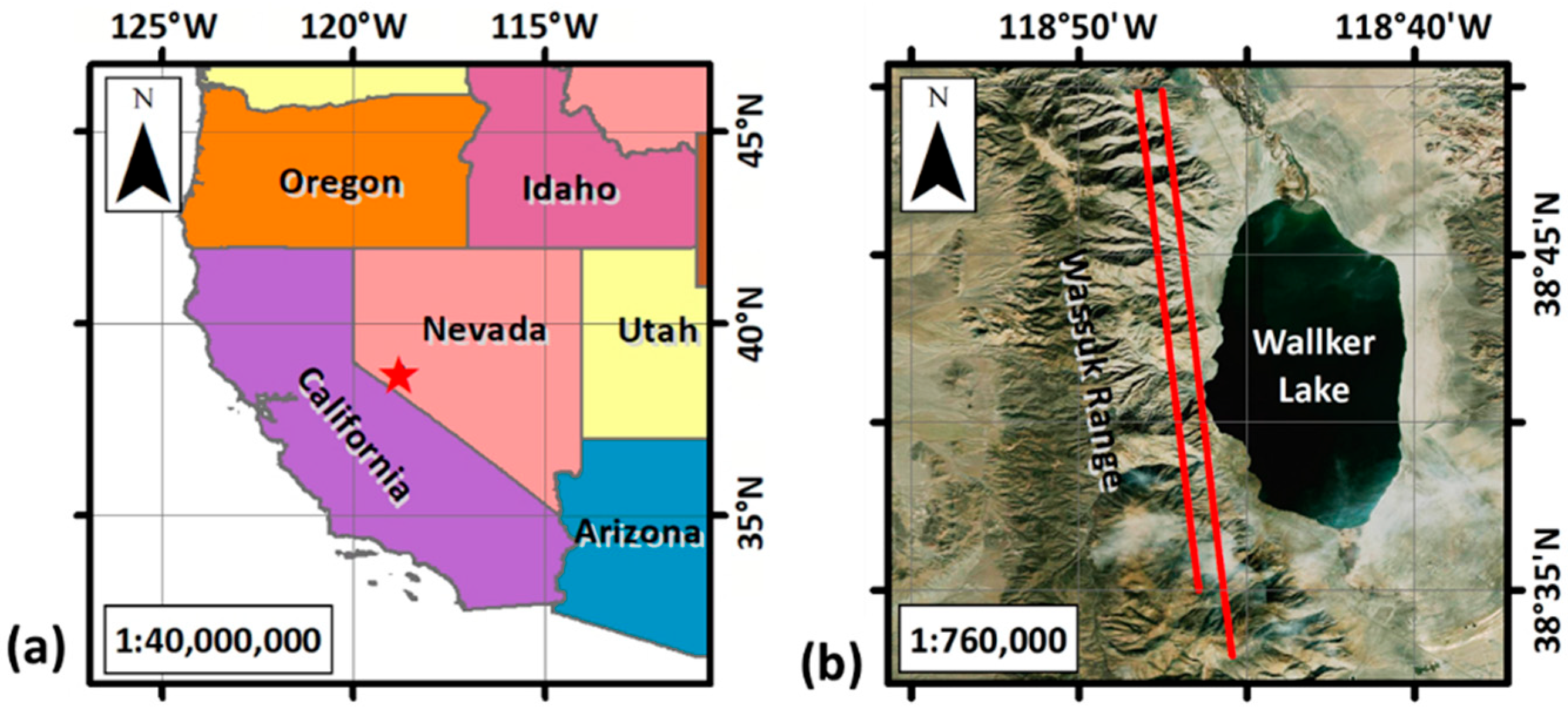
2.1. Study Area

The study area is located at western Nevada, USA with the center at [118°46′W, 38°41′N], which is marked by a red star symbol in Figure 1a. In this study site, the topography changes dramatically and the vegetation is sparsely distributed. The two tracks of the ICESat-2 lidar passing through the Wassuk Range mountain are selected, which are located to the west bank of the Walker Lake as illustrated in Figure 1b. The along-track lengths of the two selected tracks are 16 km and 17 km, respectively. The topographic elevation ranges from 1200 m to 2200 m and the across-track slope varies from 0° to 75° along the track. The complicated topography makes the selected study site suitable for testing the performance of the proposed algorithm.

2.2. ICESat-2 Data

The ICESat-2 mission has published different data products with three levels. This study employs the ATL03 product and the ATL08 product observed on 7 May 2020 and 4 May 2022, which can be collected from the National Snow and Ice Data Center website (https://search.earthdata.nasa.gov/search, accessed on 11 July 2024). The ATL03 product provides the time tag, longitude, latitude, elevation of each photon, and the noise rate. The ATL08 product gives the classification label for each ATL03 geolocated photon event including the signal labels of the ground, canopy, and canopy top as well as the noise label [57]. The ATL03 and ATL08 product can be linked by the time tag of the recorded photon event. Figure 2a gives an illustration of the ICESat-2 photon data for one selected ground track at the study area. The red points denote the signal photons and the black points denote the noise photons, which are labeled from the ATL08 product. It is apparent that the signal photons can represent the topographic relief in the along-track direction. Then, the photon data are divided into several successive segments with an along-track distance of 20 m and an along-track interval of 10 m as shown in Figure 2b. There are 3518 segments in total for the selected ground track. An enlarged view of the photon data within the green rectangle in Figure 2a and the segment partition is presented in Figure 2b. The centroid of each segment is marked by a yellow circle, whose elevation is the mean of all ground photons within the current segment.

2.3. ALS Data

The airborne laser scanner (ALS) data are used to evaluate the performance of our proposed algorithm. The ALS data at the study site originate from the U.S. Geological Survey (USGS). To completely cover the region of the ground track, the cover area of the ALS data is much larger than the ICESat-2 ground track boundary. The average ALS points density is 33 samples per square meter. The high-quality and high-density ALS data represent three-dimensional topography at the study site, which can be downloaded from the USGS website (https://apps.nationalmap.gov/downloader, accessed on 11 July 2024).

To validate the accuracy of the derived across-track slope, the ALS data are adopted to generate the reference value of the across-track slope. At each ICESat-2 segment in Figure 2, the ALS data within a square window with a length of 20 m and an interval of 10 m, whose center point is identical to the centroid of current ICESat-2 segment, are collected. The collected ALS points are fitted to a plane and the arctangent value of the fitted plane gradient in the across-track direction is treated as the reference across-track slope. We divide the reference across-track slopes into five sections: (a) 0–10°; (b) 10–20°; (c) 20–30°; (d) 30–40°, and (e) >40°. The ICESat-2 segment numbers within each slope section are counted and shown in

Table 1. Selected segment numbers within each slope section.

Across-Track Slope Range (°)	0–10	10–20	20–30	30–40	>40
Segment number	366	988	1029	829	306

. The reference across-track slopes mostly range between 10° and 40°, which reflects that the topographies along the selected ground tracks are rugged.

3. Methods

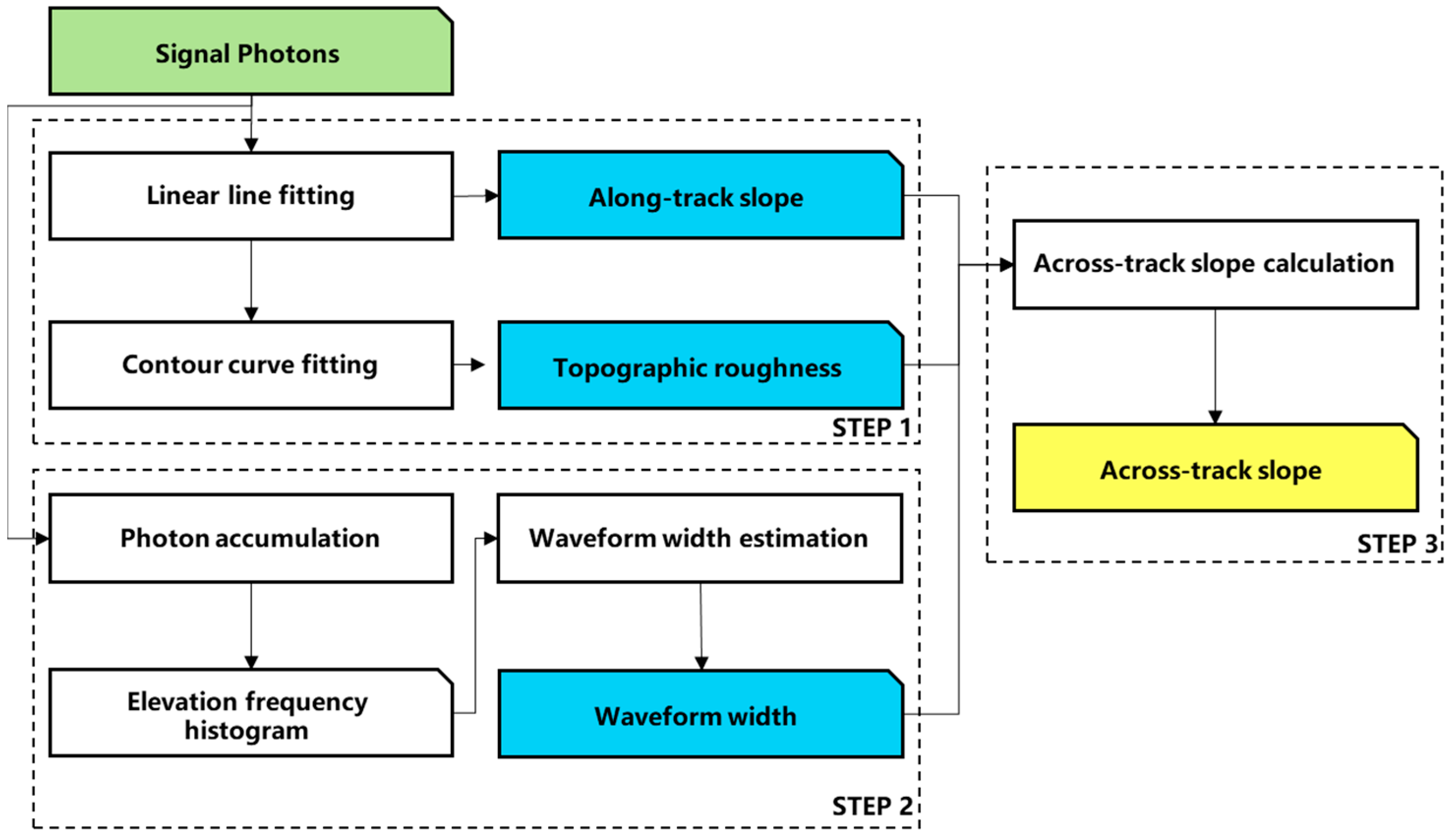
3.1. Retrieval of Across-Track Slope

The spatial distribution of the photon cloud data from a single strong beam ICESat-2 track contains enough landform geographic features to independently derive the across-track slopes. The proposed algorithm is a theory-driven method, which retrieves the across-track slope based on the root mean square (RMS) width of the Elevation Frequency Histogram from single-track photon data. It can eliminate the dependence on the dual-beam (strong and weak) data. The algorithm comprises three main steps: (1) deriving the along-track slope and topographic roughness; (2) generating the EFH and estimating the pulse width; and (3) calculating the across-track slope. It is primarily proposed for the topographic slope estimation over the bare-earth surfaces, i.e., no vegetation or buildings. The detailed flowchart of the proposed algorithm is illustrated in Figure 3.

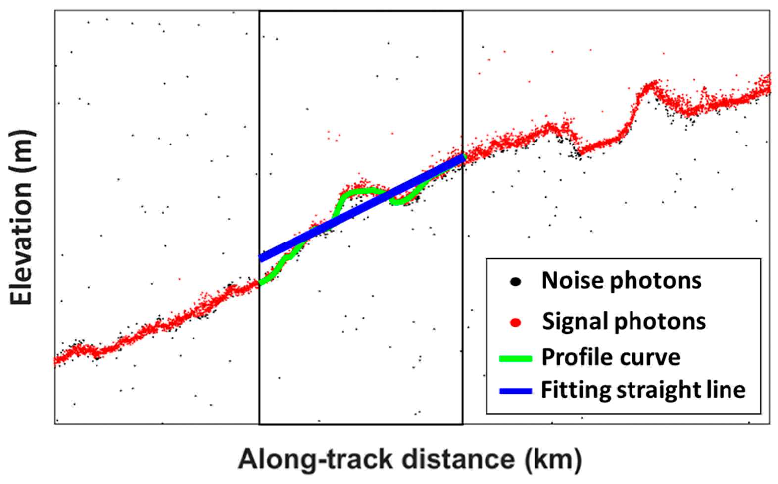
3.1.1. Deriving Along-Track Slope and Roughness Based on Photon Data

Both the topographic slope and the roughness are the key factors to determine the pulse width of the lidar received waveform. The accurate acquisition of the along-track slope and the topographic roughness is essential to the premise of the across-track slope estimation. Figure 4 illustrates the schematic for deriving the along-track slope and topographic roughness. For each segment, the ground photons labeled by the ATL08 product are utilized to generate a straight line based on the linear fitting method and a profile curve based on the median filtering method.

The fitted straight line can represent the general distribution of the ground photons in the along-track direction. The gradient of the fitted line is regarded as the along-track slope and can be given by

$$f\left(x\right)=kx+b,$$

(1)

$$S_x=\mathrm{a}\mathrm{r}\mathrm{c}\mathrm{t}\mathrm{a}\mathrm{n}\left(k\right),$$

(2)

where f(x) is the fitted line, x is the along-track distance, k and b are the gradient and the intercept of the fitted line, and S_x is the along-track slope in degrees. The profile curve can provide a more detailed description of the topographic elevations from the ground photons. The topographic roughness is defined as the standard deviation of the difference between the fitted line and the profile curve, which can be expressed as

$$\epsilon =\sqrt{{\displaystyle \frac{1}{n}}{\sum }_{i=1}^n\left(H_i-k{x}_i+b\right)}$$

(3)

where H_i represents the elevation of the profile curve for each photon, obtained using median filtering with a window size of 10 m and n is the total photon point number within each segment.

3.1.2. Generating EFH Based on Photon Data

The received waveform is the fundamental data for deriving the across-track slope. Although the Photon-Counting Lidars can only produce discrete photon data rather than analog waveform data, the EFH based on the signal photons might be regarded as the substitution for the received waveform [58]. The EFH would be produced by accumulating the ground photons within one footprint-scale (e.g., 20 m in this study) and an elevation resolution of 0.1 m. Gardner proposed a theoretical expression of the lidar signal waveform over the diffuse ground target [59]. The temporal moments of the waveform are related to the sample statistics of the topographic profile. Specifically, the RMS pulse width of the waveform is related to its normalized second-order moment and can be calculated by a series of equations [59].

$${\delta }_p^2={\displaystyle \frac{1}{N}}{\int }_0^{\infty }{(t-T_p)}^{2}p\left(t\right)dt$$

(4)

$$N={\int }_0^{\infty }p\left(t\right)dt$$

(5)

$$T_p={\displaystyle \frac{1}{N}}{\int }_0^{\infty }tp\left(t\right)dt$$

(6)

N is the total photon number of a waveform, T_p is the temporal centroid, δ_r is the RMS width, and p(t) is the waveform amplitude. If the waveform is substituted by the EFH, the pulse width can be approximately obtained using Equation (4). Specifically, the waveform amplitude p(t) is replaced by the photon count per elevation bin of the EFH and t is the time tag corresponding to the photon elevation.

3.1.3. Estimating Across-Track Slope Based on EFH Waveform

The lidar system transmits a laser beam onto the land surface, and the distribution of the received pulse is strongly correlated with the landform geography. According to the received signal model of the full-waveform lidar, the mean-square pulse width of the received waveform is related to topographic relief due to the surface slope and roughness, which can be expressed as follows [60]:

$${\delta }_p^2={\delta }_f^2+{\delta }_r^2+{\displaystyle \frac{4{\epsilon }^2{\mathrm{c}\mathrm{o}\mathrm{s}}^2{S}_x}{c^2{\mathrm{c}\mathrm{o}\mathrm{s}}^2\left(S_x+\phi \right)}}+{\displaystyle \frac{4r^2}{c^2{\mathrm{c}\mathrm{o}\mathrm{s}}^2\phi }}\left[{\mathrm{t}\mathrm{a}\mathrm{n}}^2{\theta }_T+{\mathrm{t}\mathrm{a}\mathrm{n}}^2\left(S_x+\phi \right)+{\displaystyle \frac{{\mathrm{t}\mathrm{a}\mathrm{n}}^2{S}_y{\mathrm{c}\mathrm{o}\mathrm{s}}^2{S}_x}{{\mathrm{c}\mathrm{o}\mathrm{s}}^2\left(S_x+\phi \right)}}\right],$$

(7)

where δ_f is the RMS pulse width of the transmitted laser pulse, δ_r is the RMS width of the receiver impulse response, c is the velocity of light, φ is the off-nadir laser pointing angle, θ_T is the RMS laser divergence angle, and S_y is the across-track slope. As the laser divergence angle and the off-nadir laser pointing angle are generally much less than the surface slope, the terms regarding ϕ and θ_T can be ignored. Hence, the mean-square pulse width of the received signal can be simplified as

$${\delta }_p^2={\delta }_f^2+{\delta }_r^2+{\displaystyle \frac{4{\epsilon }^2}{c^2}}+{\displaystyle \frac{4r^2}{c^2}}\left({\mathrm{t}\mathrm{a}\mathrm{n}}^2{S}_x+{\mathrm{t}\mathrm{a}\mathrm{n}}^2{S}_y\right).$$

(8)

Solving Equation (8) for S_y, we obtain the following expression for the across-track slope.

$$S_y=\arctan \left[{\displaystyle \frac{\cos \left(S_x+\phi \right)}{\cos S_x}}\sqrt{{\displaystyle \frac{c^2}{4r^2}}\left({\delta }_p^2-{\delta }_f^2-{\delta }_r^2-{\displaystyle \frac{4{\epsilon }^2}{c^2}}\right)-{\mathrm{t}\mathrm{a}\mathrm{n}}^2{S}_x}\right].$$

(9)

As for the PCL, the RMS widths of the transmitted laser pulse and the receiver impulse response are given. In addition, the along-track slope and the topographic roughness can be estimated from Equation (2) and Equation (3), respectively. Hence, once the RMS pulse width of the EFH is determined using Equation (4), the footprint-scale across-track slope can be derived based on Equation (9) just using the single-track photon data (only the strong beam data are used).

3.2. Accuracy Validation

To evaluate the accuracies of the retrieved across-track slopes, three indicators including mean absolute error (MAE), root mean square error (RMSE), and mean of the slope residuals (MEAN) are introduced as

$$\mathrm{M}\mathrm{A}\mathrm{E}={\displaystyle \frac{1}{m}}\sum _{i=1}^m\left|{rs}_i-{ds}_i\right|,$$

(10)

$$\mathrm{R}\mathrm{M}\mathrm{S}\mathrm{E}=\sqrt{{\displaystyle \frac{1}{m}}\sum _{i=1}^m{\left({rs}_i-{ds}_i\right)}^2},$$

(11)

$$\mathrm{M}\mathrm{E}\mathrm{A}\mathrm{N}={\displaystyle \frac{1}{m}}\sum _{i=1}^m\left({rs}_i-{ds}_i\right),$$

(12)

where rs_i represents the derived across-track slope from the ICESat-2 photon data, and ds_i represents the reference across-track slope from the airborne laser scanner (ALS) data. m is the valid segment number (the invalid instances will be defined in following section). Moreover, to further assess the topographic applicability of our proposed algorithm, three additional indicators including the median, the inter quartile range (IQR), and the whisker range (the range of the residuals) [61] are calculated according to the slope residuals under different slope sections in Table 1. To further test the applicability of our retrieved across-track slope, the ICESat-2 team’s method [53] and the plane fitting method [50] would be conducted for comparison. For consistency, all methods derive the across-track slope using an along-track length of 20 m and an interval of 10 m, matching the resolution of the ALS data.

4. Results and Discussion

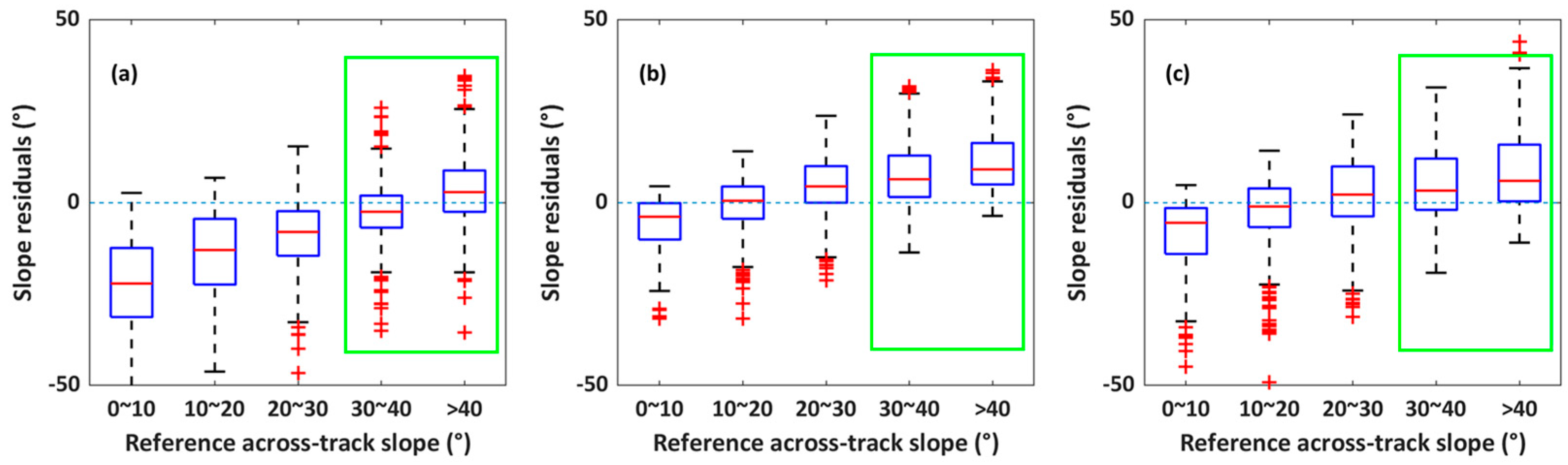
4.1. Accuracy of Retrieved Across-Track Slope

Figure 5 illustrates the retrieved results of the across-track slopes compared to those ALS reference values by different methods. The scattered points in Figure 5a–c are produced by our method, the ICESat-2 team’s method, and the plane fitting method, respectively. The colors of the scatter points represent the point density distributions, where the red points and blue points correspond to the dense and sparse densities, respectively. The red ellipses represent high confidence, i.e., regions where the point density exceeds 10 in this study. The x-shape points denote the invalid instances under the following circumstances for different methods: (a) the across-track slope is set to 0 when the radicand in Equation (9) is less than 0 (our method); (b) the across-track slope is set to 0 when the photon data of the weak-beam are missed (the ICESat-2 team method and the plane fitting method); (c) the across-track slopes have bigger errors when the photon geolocation accuracies of the weak-beam are inferior, particularly when the elevation range of the signal photons differs significantly from that of the strong-beam (the plane fitting method).

The confidence regions created by our method in Figure 5a have denser concentrations near the 1:1 line when the reference across-track slopes range from 20° to 40°. The scattered points around the 30° reference across-track slope have maximum point densities. The retrieved across-track slopes are apparently overestimated as the reference across-track slopes are less than 20°. The invalid points may be caused by the inaccurate estimations of the pulse width and will be explored in the Discussion section. The retrieved across-track slopes by the ICESat-2 team method and the plane fitting method in Figure 5b,c are generally satisfactory. However, invalid points have a notable increment relative to those obtained by our method. To further investigate the quantitative discrepancy between the retrieved across-track slopes and the ALS reference values, the accuracy evaluation indicators including the MAE, MEAN, and RMSE are calculated and listed in

Table 2. Accuracy evaluation of the retrieved across-track slopes using our method, ICESat-2 team method, and the plane fitting method.

	MAE	RMSE	MEAN	Invalid Segment
Our method	11.45°	10.45°	−8.26°	88 (2.51%)
ICESat-2 team method	11.61°	10.61°	8.90°	1137 (32.32%)
Plane fitting method	12.51°	10.53°	−2.67°	362 (10.29%)

.

It can be observed that our method produces a minimum MAE and RMSE of 11.45° and 10.45°, which are comparable to those obtained by the ICESat-2 team method and the plane fitting method. However, our method has an apparent overestimation of the across-track slope with a MEAN of −8.26°. On the other hand, the ICESat-2 team method demonstrates a greater underestimation of the across-track slope with the MEAN of 8.90°. The plane fitting method has the most superior MEAN of −2.67°. In addition, the invalid segment numbers and proportions to the total segment number of 3518 are counted. Our proposed method yields the least invalid segments of 88 corresponding to the proportion of 2.51%, significantly outperforming both the plane fitting method (362 invalid segments and 10.29% proportion) and the ICESat-2 team method (1137 invalid segments and 32.32% proportion).

The high invalid instances of the ICESat-2 team and the plane fitting method may arise from the background noise. The selected dataset was acquired during the daytime, when the signal-to-noise ratio is relatively low due to the solar background noise. As a result, the signal photons for the weak beam segments are frequently undetected, making it impossible to either perform the plane fitting or calculate reliable elevation differences in a beam pair. These cases are thus marked as “invalid” instances (i.e., lacking valid photon data from a beam pair). The quantitative analyses indicate that our method, based on single-track photon data of the strong beam, has similar across-track slope accuracies to the other two methods, which relied on multi-track photon data. Furthermore, our method can provide more valid measurements of the across-track slopes with higher resolution (20 m scale close to the footprint size rather than 90 m scale between the strong and weak beam).

4.2. Topographic Applicability Assessment

Rugged topography is the major challenge in the extraction of the across-track slopes. To verify the topographic applicability of our method, we investigate the accuracy of the retrieved across-track slopes under different reference across-track slopes. Figure 6 illustrates the relationship between the residuals of the across-track slopes and the reference across-track slopes. It is noticed that the results in Figure 6 are only based on the valid instances. When the reference across-track slopes are less than 20°, the accuracies of the retrieved across-track slopes by our method are relatively worse than those obtained by the other two methods. However, with the increment of the reference across-track slopes, the accuracies of the retrieved across-track slopes by our method are improved. The medians of the slope residuals obtained by our method decrease rapidly and are less than those obtained by the ICESat-2 team method or the plane fitting method when the reference across-track slopes are greater than 30°. The IQR and the whisker ranges obtained by our method gradually reduce as well and are basically equivalent to those obtained by the other two methods when the reference across-track slopes exceed 20°. It demonstrates that our method could improve the accuracies of the across-track slopes over the rugged topography.

Furthermore,

Table 3. Median, IQR, and whisker range of the retrieved across-track slopes using our method, ICESat-2 team method, and plane fitting method under different across-track slope sections.

Methods	Indicators	Reference Across-Track Slope (°)
		0–10	10–20	20–30	30–40	>40
Our method	Median	−22.10	−12.93	−7.98	−2.47	2.90
	IQR	18.89	17.96	12.19	8.75	11.32
	Whisker range	54.77	56.15	48.21	35.02	45.26
ICESat-2 team method	Median	−3.84	0.55	4.47	6.43	9.12
	IQR	9.96	8.84	10.01	11.34	11.34
	Whisker range	29.51	31.74	38.77	43.52	36.96
Plane fitting method	Median	−5.49	−1.03	2.23	3.32	5.99
	IQR	12.56	10.60	13.66	14.01	15.51
	Whisker range	37.67	36.80	48.38	50.72	50.07

presents the median, the IQR, and the whisker under different slope sections based on the valid data in Figure 6. When the reference across-track slopes are less than 20°, our method performs significantly worse than both the ICESat-2 team method and the plane fitting method. The average differences in the absolute median, the IQR, and the whisker range are greater than 14.25°, 6.84°, and 18.23°, relative to the other two methods. Such differences tend to be decreased when the reference across-track slopes exceed 20°. When the reference across-track slopes range from 20° to 30°, the absolute differences in the median, the IQR, and the whisker range decrease to less than 5.75°, 2.18°, and 9.43°. As the reference across-track slopes are greater than 30°, our method can consistently yield the optimal across-track slopes with the minimal median, IQR, and whisker range (except for the whisker range by the ICESat-2 team method). The average reductions in the absolute median, IQR, and whisker range are greater than 4.44°, 1.31° and 0.10°, respectively. The quantitative indicators in Table 3 prove once again that our method can obtain higher-precision across-track slopes over the steep terrain.

Additionally, invalid segments (marked by x-points in Figure 5) and outliers (marked by red crosses in Figure 6 are divided into five slope sections.

Table 4. Invalid and outlier numbers of the retrieved across-track slopes using our method, ICESat-2 team method, and plane fitting method under different reference across-track slope sections.

Methods	Factors	Reference Across-Track Slope (°)
		0–10	10–20	20–30	30–40	>40
Our method	Invalid	6 (1.64%)	24 (2.43%)	25 (2.43%)	19 (2.29%)	14 (4.58%)
	Outliers	0 (0%)	1 (0.10%)	5 (0.49%)	21 (2.53%)	13 (4.25%)
ICESat-2 team method	Invalid	100 (27.32%)	334 (34.82%)	290 (28.18%)	265 (31.97%)	148 (48.04%)
	Outliers	5 (1.37%)	11 (1.11%)	8 (0.78%)	6 (0.72%)	4 (1.31%)
Plane fitting method	Invalid	22 (6.01%)	96 (9.72%)	88 (8.55%)	100 (12.06%)	56 (18.30%)
	Outliers	7 (1.91%)	19 (1.92%)	7 (0.68%)	0 (0%)	4 (1.31%)

lists the numbers of the invalid segments and outliers by three methods. The number of outliers is less than the invalid segments for all three methods, and the numbers of outliers from three methods are comparable. However, there are significant discrepancies regarding the invalid segments by different methods. The ICESat-2 team method yields the maximal invalid segments and our method yields the minimal invalid segments. The proportions of the invalid segments by the ICESat-2 team method remain at a level of about 30%. The plane fitting method gives such proportions ranging from 6.01% to 18.30%, with the increase in the reference across-track slopes. The proportions by our method are much less than the other two methods and are less than 4.58% for all slope sections. The results imply that our method can provide more valid across-track slopes over the rugged topography.

5. Discussion

Although our proposed method can provide higher-precision and more valid across-track slopes over rugged topography, there are still two negative instances, i.e., invalid values or large-errors (defined as >40% in this paper) relative to the reference values. To explore the inherent reasons for these instances, the topographic parameters including the reference across-track slopes, along-track slopes, and topographic roughness are collected. By investigating the inner connection between the topographic parameters and the pulse width of the EFH, it is expected to expound these instances.

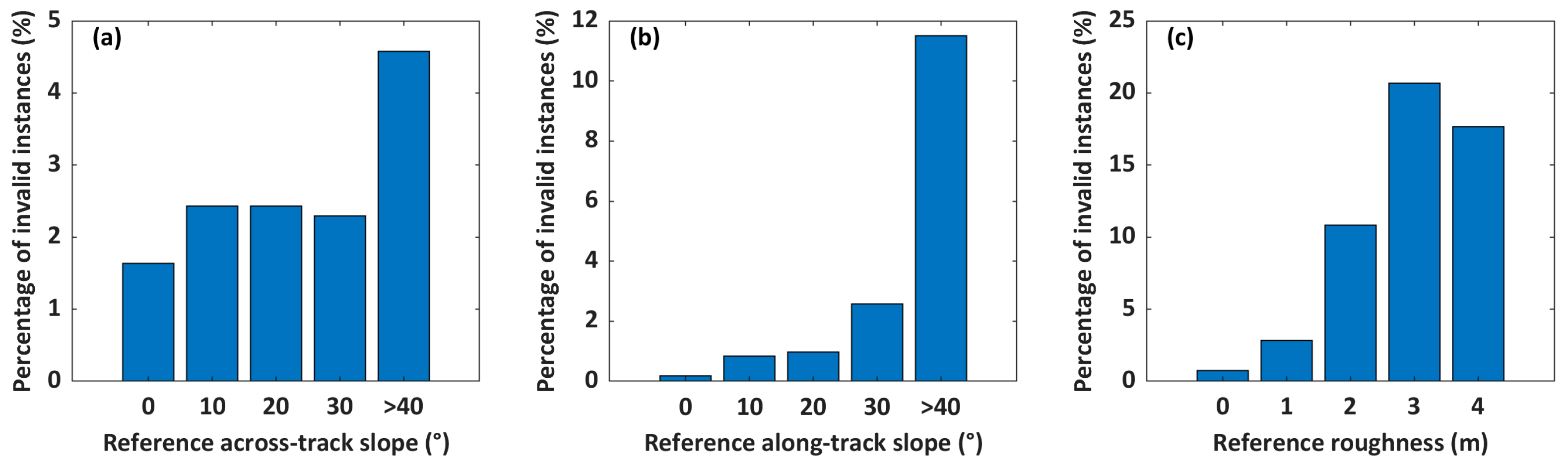
5.1. Invalid Instance Analysis

We calculate the topographic parameters under the invalid instances using the ALS data. The statistical histogram distributions of the resolved topographic parameters are presented in Figure 7. As shown in Figure 7a, the percentages of the invalid instance are less than 5% with varying reference across-track slopes. It indicates that the across-track slope might not be the main reason for the invalid instances. However, the impacts of the reference along-track slopes and topographic roughness on the invalid instances are totally different, as presented in Figure 7b,c. With the growth of the reference along-track slopes, the percentages of the invalid instance rapidly increase, especially when the along-track slopes are more than 40°. On the other hand, the influence of the bigger roughness on the invalid instances cannot be ignored either. If the roughness is more than 2 m, the percentages of the invalid instances exceed 10%. To further interpret the effects of the topographic parameters on the distributions of the actual waveform and the EFH, the ALS simulated waveforms are generated using the ALS data in Section 2.3 and the waveform simulator [62].

Figure 8 illustrates an example of the EFH and the ALS simulated waveform, under the condition that the reference across-track slope, along-track slope, and topographic roughness are 29.57°, 35.15°, and 3.31 m, respectively. The ALS simulated waveform is generated using the ALS data in Section 2.3 and the waveform simulator [62]. We observe that the range of the EFH is much less than the signal duration of the ALS simulated waveform. It means that the received pulse width of the EFH based on Equation (4) would be less than the theoretical pulse width of the ALS simulated waveform in Equation (7). Hence, the radicand in Equation (9) is a negative number, resulting in the invalid instance.

In other words, the underestimation of the received pulse width based on the EFH may lead to invalid instances. Hence, we plot the pulse width residuals between the EFH and the simulated waveform for the invalid instances, as presented in Figure 9. The pulse width residuals for the invalid instances in Figure 9a present fluctuating distribution around the zero line. The corresponding statistical histogram in Figure 9b reveals that the maximum absolute value of the negative residuals exceeds that of the positive ones. Moreover, the proportion of the pulse width underestimations for all invalid instances reaches 51.14%.

However, such a proportion is insufficient to conclude that the pulse width underestimation is the only factor for the invalid instances. To further investigate the inherent influence factors, we analyze the residuals of the along-track slopes and the surface roughness in the invalid instances, derived from both the ALS data and ICESat-2 data. Figure 10a demonstrates that the along-track slopes derived from the ICESat-2 data closely approach the reference values from the ALS data, with a mean residual of −0.24° and a standard deviation of 14.59°. In contrast, Figure 10b reveals an apparent overestimation of the surface roughness by the ICESat-2 data, with a mean residual of 0.92 m and a standard deviation of 1.65 m. According to Equation (9), such an overestimation of the roughness would lead to a reduction in the across-track slope, thereby increasing the likelihood of the invalid instances. These findings suggest that the overestimated surface roughness may play a significant role in the occurrence of invalid instances as well.

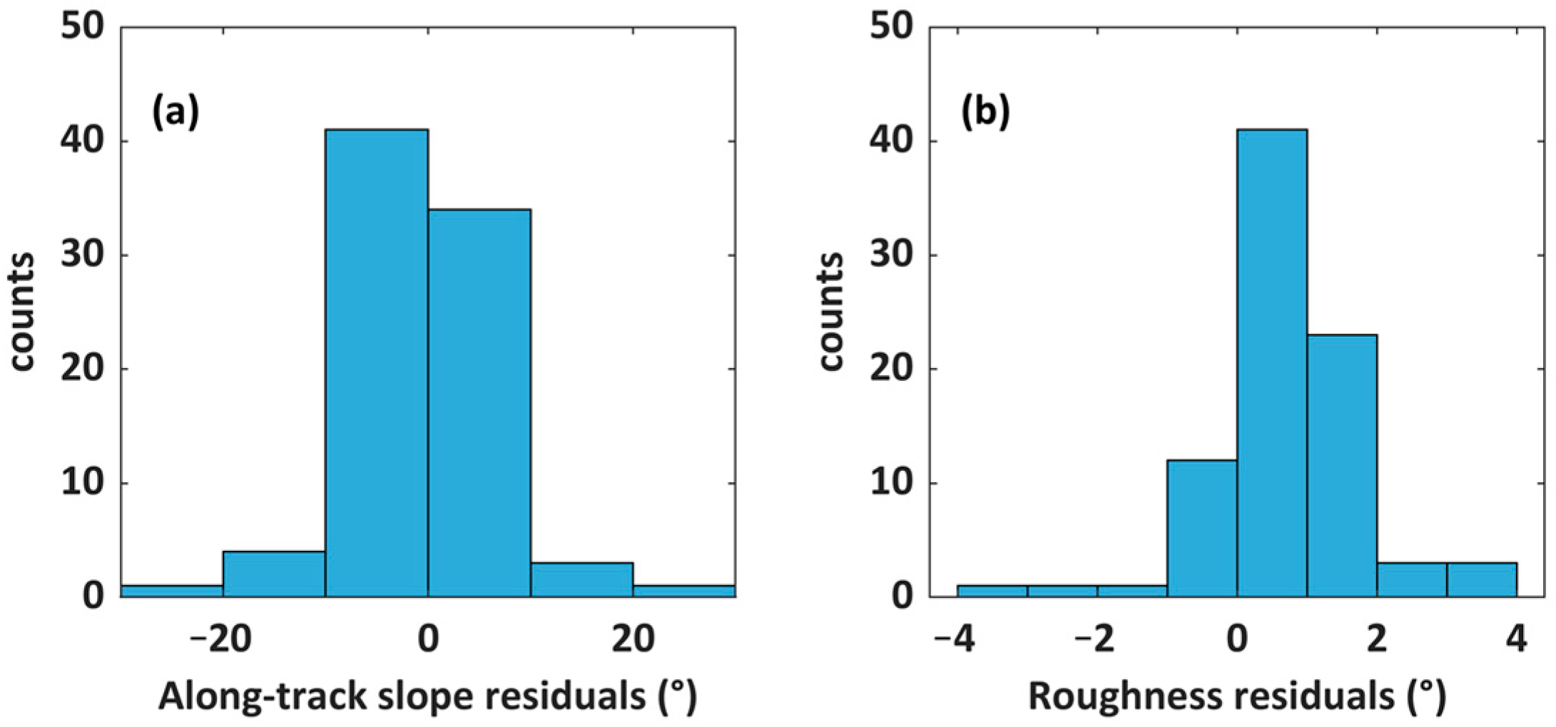
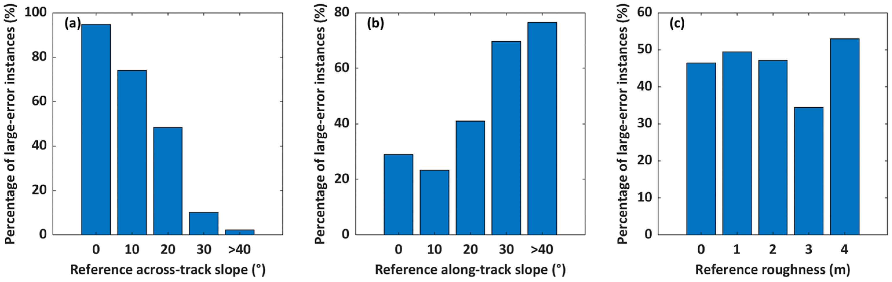
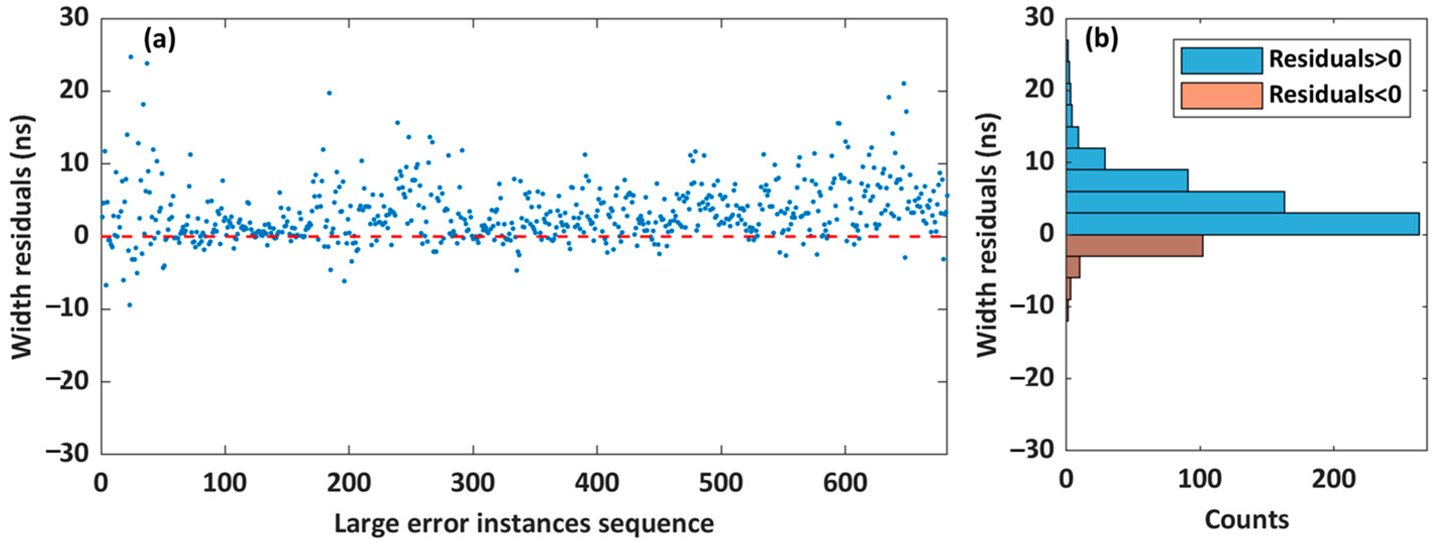
5.2. Large-Error Instance Analysis

Just like the invalid instance, we also calculate the topographic parameters for the large-error instances. Figure 11 illustrates the statistical histogram distributions of the large-error instances for different topographic parameters. The percentages in Figure 11a have the opposite distribution regularities to the percentages of the invalid instances in Figure 7a, with the increment of the reference across-track slopes. The percentages in Figure 11b show an upward trend with an increase in the reference along-track slopes. When the across-track slopes are less than 30°, the large-error instances are prevalent. However, the percentages in Figure 11c present relatively stable distributions for different roughness values, indicating that the large-error instances are insensitive to the topographic roughness.

The large-error instances may be caused by the overestimation of the received pulse width from the EFH. We give an illustration of the EFH and ALS simulated waveform as shown in Figure 12, when the reference across-track slope, along-track slope, and topographic roughness are 49.57°, 39.79°, and 4.56 m, respectively. In Figure 12, the EFH waveform exhibits a distinct comb-shaped distribution whereas the ALS simulated waveform presents a multimodal distribution. Compared with the simulated waveform, the EFH demonstrates irregular amplitude variations and displays evident truncation at both the start and end times. The range of the EFH is greater than that of the ALS simulated waveform. Hence, the pulse width of the EFH would exceed the theoretical pulse width of the simulated waveform. The overestimation of the received pulse width based on the EFH may result in a large-error instance.

To further expound the influence of the pulse width overestimation on the large-error instances, the pulse width residuals between the EFH and ALS simulated waveform for large-error instances are illustrated in Figure 13. The pulse width residuals for the large-error instances in Figure 13a are basically distributed above the zero line. The corresponding statistical histogram in Figure 13b indicates that the large-error instances chiefly occur when the pulse width residual is positive (with the pulse width overestimation). The proportion of the pulse width overestimations for all large-error instances reaches 82.99%.

We also intend to interpret this issue from a mathematical perspective. As presented in Equation (8), the along-track slope and the across-track slope have equivalent contributions to the pulse width of the received waveform. If the roughness is neglected and the along-track slope is fixed, the relationship between the pulse width and the across-track slope is as shown in Figure 14. As illustrated in Figure 14a, as for an identical window of the pulse width, the growth of the across-track slope before the inflection point (where the across-track slope equals to the along-track slope) is greater than the growth after the inflection point. It implies that the derived across-track slope has considerable uncertainty for a given pulse width error, when the actual across-track slope is smaller than the actual along-track slope. Furthermore, such uncertainties tend to increase with the increment of the along-track slope, as presented in Figure 14b. These results demonstrate that the derived across-track slopes by the ICESat-2 photon data are particularly sensitive to the small discrepancies in pulse width for the higher along-track slopes, leading to relatively large errors when deriving across-track slopes.

In general, when the topographic parameters are variable, the estimated pulse widths from the EFH may have different accuracies, which is the primary reason leading to the uncertainty of retrieved across-track slopes. To improve the retrieval accuracy of the across-track slope, it is worth investigating more efficient methods for pulse width estimation by the EFH in the future.

6. Conclusions

We propose a new method to retrieve across-track slopes based on the RMS width of the EFH from the ICESat-2 single-track photon data of a strong beam. By comparing the retrieved across-track slopes by our method with those obtained by the ICESat-2 team official approach and the plane fitting method, our method can achieve comparable retrieved accuracy but more valid and higher-resolution results for diverse topographic features. When the reference across-track slopes exceed 30°, our method can consistently yield the optimal retrieved across-track slopes with maximum valid values and highest precision. It demonstrates that our method has better applicability for deriving the across-track slopes over rugged terrains.

Compared with the open-source global DEMs, such as the SRTM DEM or ASTER GDEM, the proposed approach can offer higher-precision and higher-resolution surface slopes. This makes it well-suited for detecting terrain changes in landslide scars and active mining areas. However, our method also produces some negative instances including invalid and large-error across-track slopes under different topographic parameters. By investigating the pulse width residuals between the EFH and the simulated waveform, the invalid instances are mainly caused by the underestimation of the received pulse width from the EFH. On the contrary, the large-error instances are chiefly induced by the received pulse width overestimation. The inaccurate estimations of the pulse width from the EFH may be attributed to the shape deviation between the EFH and the full waveform. Hence, it is a challenge to extract the accurate pulse width from the discrete and sparse PCL photon data, which is beneficial to improve the retrieval accuracy of the across-track slope.

References

1. Hilbert, C.; Schmullius, C. Influence of Surface Topography on ICESat/GLAS Forest Height Estimation and Waveform Shape. Remote Sens. 2012, 4, 2210–2235. [Google Scholar] [CrossRef]
2. del Rosario Gonzalez-Moradas, M.; Viveen, W. Evaluation of ASTER GDEM2, SRTMv3. 0, ALOS AW3D30 and TanDEM-X DEMs for the Peruvian Andes against Highly Accurate GNSS Ground Control Points and Geomorphological-Hydrological Metrics. Remote Sens. Environ. 2020, 237, 111509. [Google Scholar] [CrossRef]
3. Fricker, G.A.; Synes, N.W.; Serra-Diaz, J.M.; North, M.P.; Davis, F.W.; Franklin, J. More than Climate? Predictors of Tree Canopy Height Vary with Scale in Complex Terrain, Sierra Nevada, CA (USA). For. Ecol. Manag. 2019, 434, 142–153. [Google Scholar] [CrossRef]
4. Eitel, J.U.; Höfle, B.; Vierling, L.A.; Abellán, A.; Asner, G.P.; Deems, J.S.; Glennie, C.L.; Joerg, P.C.; LeWinter, A.L.; Magney, T.S. Beyond 3-D: The New Spectrum of Lidar Applications for Earth and Ecological Sciences. Remote Sens. Environ. 2016, 186, 372–392. [Google Scholar] [CrossRef]
5. Muscarella, R.; Kolyaie, S.; Morton, D.C.; Zimmerman, J.K.; Uriarte, M. Effects of Topography on Tropical Forest Structure Depend on Climate Context. J. Ecol. 2020, 108, 145–159. [Google Scholar] [CrossRef]
6. Yu, J.; Liu, H.; Wang, L.; Jezek, K.C.; Heo, J. Blue Ice Areas and Their Topographical Properties in the Lambert Glacier, Amery Iceshelf System Using Landsat ETM+, ICESat Laser Altimetry and ASTER GDEM Data. Antarct. Sci. 2012, 24, 95–110. [Google Scholar] [CrossRef]
7. Giardino, M.; Perotti, L.; Lanfranco, M.; Perrone, G. GIS and Geomatics for Disaster Management and Emergency Relief: A Proactive Response to Natural Hazards. Appl. Geomat. 2012, 4, 33–46. [Google Scholar] [CrossRef]
8. Cao, G.; Wei, X.; Ye, J. Fireground Recognition and Spatio-Temporal Scalability Research Based on ICESat-2/ATLAS Vertical Structure Parameters. Forests 2024, 15, 1597. [Google Scholar] [CrossRef]
9. Evans, I.S. Geomorphometry and Landform Mapping: What Is a Landform? Geomorphology 2012, 137, 94–106. [Google Scholar] [CrossRef]
10. Schillaci, C.; Braun, A.; Kropáček, J. Terrain Analysis and Landform Recognition. In Geomorphological Techniques (Online Edition); Clarke, N.E., Nield, J.M., Eds.; British Society for Geomorphology: London, UK, 2015. [Google Scholar]
11. Zhao, G.; Xue, H.; Ling, F. Assessment of ASTER GDEM Performance by Comparing with SRTM and ICESat/GLAS Data in Central China. In Proceedings of the 2010 18th International Conference on Geoinformatics, Beijing, China, 18–20 June 2010; pp. 1–5. [Google Scholar]
12. Carabajal, C.C.; Harding, D.J. SRTM C-Band and ICESat Laser Altimetry Elevation Comparisons as a Function of Tree Cover and Relief. Photogramm. Eng. Remote Sens. 2006, 72, 287–298. [Google Scholar] [CrossRef]
13. Braun, A.; Fotopoulos, G. Assessment of SRTM, ICESat, and Survey Control Monument Elevations in Canada. Photogramm. Eng. Remote Sens. 2007, 73, 1333–1342. [Google Scholar] [CrossRef]
14. Carabajal, C.C.; Harding, D.J. ICESat Validation of SRTM C-Band Digital Elevation Models. Geophys. Res. Lett. 2005, 32, 22. [Google Scholar] [CrossRef]
15. Wessel, B.; Huber, M.; Wohlfart, C.; Marschalk, U.; Kosmann, D.; Roth, A. Accuracy Assessment of the Global TanDEM-X Digital Elevation Model with GPS Data. ISPRS J. Photogramm. Remote Sens. 2018, 139, 171–182. [Google Scholar] [CrossRef]
16. Rizzoli, P.; Martone, M.; Gonzalez, C.; Wecklich, C.; Tridon, D.B.; Bräutigam, B.; Bachmann, M.; Schulze, D.; Fritz, T.; Huber, M. Generation and Performance Assessment of the Global TanDEM-X Digital Elevation Model. ISPRS J. Photogramm. Remote Sens. 2017, 132, 119–139. [Google Scholar] [CrossRef]
17. Liu, A.; Cheng, X.; Chen, Z. Performance Evaluation of GEDI and ICESat-2 Laser Altimeter Data for Terrain and Canopy Height Retrievals. Remote Sens. Environ. 2021, 264, 112571. [Google Scholar] [CrossRef]
18. Mallet, C.; Bretar, F. Full-Waveform Topographic Lidar: State-of-the-Art. ISPRS J. Photogramm. Remote Sens. 2009, 64, 1–16. [Google Scholar] [CrossRef]
19. Magruder, L.A.; Brunt, K.M. Performance Analysis of Airborne Photon- Counting Lidar Data in Preparation for the ICESat-2 Mission. IEEE Trans. Geosci. Remote Sens. 2018, 56, 2911–2918. [Google Scholar] [CrossRef]
20. Schutz, B.E.; Zwally, H.J.; Shuman, C.A.; Hancock, D.; DiMarzio, J.P. Overview of the ICESat Mission. Geophys. Res. Lett. 2005, 32, L21S01. [Google Scholar] [CrossRef]
21. Wang, X.; Cheng, X.; Gong, P.; Huang, H.; Li, Z. and Li, X. Earth Science Applications of ICESat/GLAS: A Review. Int. J. Remote Sens. 2011, 32, 8837–8864. [Google Scholar] [CrossRef]
22. Kwok, R.; Zwally, H.J.; Yi, D. ICESat Observations of Arctic Sea Ice: A First Look. Geophys. Res. Lett. 2004, 31, 16. [Google Scholar] [CrossRef]
23. Markus, T.; Neumann, T.; Martino, A.; Abdalati, W.; Brunt, K.; Csatho, B.; Farrell, S.; Fricker, H.; Gardner, A.; Harding, D. The Ice, Cloud, and Land Elevation Satellite-2 (ICESat-2): Science Requirements, Concept, and Implementation. Remote Sens. Environ. 2017, 190, 260–273. [Google Scholar] [CrossRef]
24. Neumann, T.A.; Brenner, A.C.; Hancock, D.W.; Harbeck, K.; Luthcke, S.; Robbins, J.; Saba, J.; Gibbons, A. Ice, Cloud, and Land Elevation Satellite-2 Project Algorithm Theoretical Basis Document for Global Geolocated Photons (ATL03); NASA Goddard Space Flight Center: Greenbelt, MD, USA, June 2018. [Google Scholar]
25. Patterson, P.L.; Healey, S.P.; Ståhl, G.; Saarela, S.; Holm, S.; Andersen, H.-E.; Dubayah, R.O.; Duncanson, L.; Hancock, S.; Armston, J. Statistical Properties of Hybrid Estimators Proposed for GEDI—NASA’s Global Ecosystem Dynamics Investigation. Environ. Res. Lett. 2019, 14, 065007. [Google Scholar] [CrossRef]
26. Potapov, P.; Li, X.; Hernandez-Serna, A.; Tyukavina, A.; Hansen, M.C.; Kommareddy, A.; Pickens, A.; Turubanova, S.; Tang, H.; Silva, C.E.; et al. Mapping Global Forest Canopy Height through Integration of GEDI and Landsat Data. Remote Sens. Environ. 2021, 253, 112165. [Google Scholar] [CrossRef]
27. Shendryk, Y. Fusing GEDI with Earth Observation Data for Large Area Aboveground Biomass Mapping. Int. J. Appl. Earth Obs. Geoinf. 2022, 115, 103108. [Google Scholar] [CrossRef]
28. Spinhirne, J.D.; Palm, S.P.; Hart, W.D.; Hlavka, D.L.; Welton, E.J. Cloud and Aerosol Measurements from GLAS: Overview and Initial Results. Geophys. Res. Lett. 2005, 32, 22. [Google Scholar] [CrossRef]
29. Magruder, L.A.; Webb, C.E.; Urban, T.J.; Silverberg, E.C.; Schutz, B.E. ICESat Altimetry Data Product Verification at White Sands Space Harbor. IEEE Trans. Geosci. Remote Sens. 2007, 45, 147–155. [Google Scholar] [CrossRef]
30. Fayad, I.; Baghdadi, N.; Frappart, F. Comparative Analysis of GEDI’s Elevation Accuracy from the First and Second Data Product Releases over Inland Waterbodies. Remote Sens. 2022, 14, 340. [Google Scholar] [CrossRef]
31. Gong, P.; Li, Z.; Huang, H.; Sun, G.; Wang, L. ICESat GLAS Data for Urban Environment Monitoring. IEEE Trans. Geosci. Remote Sens. 2011, 49, 1158–1172. [Google Scholar] [CrossRef]
32. Neumann, T.A.; Martino, A.J.; Markus, T.; Bae, S.; Bock, M.R.; Brenner, A.C.; Brunt, K.M.; Cavanaugh, J.; Fernandes, S.T.; Hancock, D.W. The Ice, Cloud, and Land Elevation Satellite–2 Mission: A Global Geolocated Photon Product Derived from the Advanced Topographic Laser Altimeter System. Remote Sens. Environ. 2019, 233, 111325. [Google Scholar] [CrossRef]
33. Magruder, L.A.; Brunt, K.M.; Alonzo, M. Early ICESat-2 on-Orbit Geolocation Validation Using Ground-Based Corner Cube Retro-Reflectors. Remote Sens. 2020, 12, 3653. [Google Scholar] [CrossRef]
34. Parrish, C.E.; Magruder, L.A.; Neuenschwander, A.L.; Forfinski-Sarkozi, N.; Alonzo, M.; Jasinski, M. Validation of ICESat-2 ATLAS Bathymetry and Analysis of ATLAS’s Bathymetric Mapping Performance. Remote Sens. 2019, 11, 1634. [Google Scholar] [CrossRef]
35. Xu, N.; Ma, Y.; Zhou, H.; Zhang, W.; Zhang, Z.; Wang, X.H. A Method to Derive Bathymetry for Dynamic Water Bodies Using ICESat-2 and GSWD Data Sets. IEEE Geosci. Remote Sens. Lett. 2020, 19, 1–5. [Google Scholar] [CrossRef]
36. Bagnardi, M.; Kurtz, N.T.; Petty, A.A.; Kwok, R. Sea Surface Height Anomalies of the Arctic Ocean from ICESat-2: A First Examination and Comparisons with CryoSat-2. Geophys. Res. Lett. 2021, 48, e2021GL093155. [Google Scholar] [CrossRef]
37. Herzfeld, U.C.; Lawson, M.; Trantow, T.; Nylen, T. Airborne Validation of ICESat-2 ATLAS Data over Crevassed Surfaces and Other Complex Glacial Environments: Results from Experiments of Laser Altimeter and Kinematic GPS Data Collection from a Helicopter over a Surging Arctic Glacier (Negribreen, Svalbard). Remote Sens. 2022, 14, 1185. [Google Scholar] [CrossRef]
38. Wang, J.; Yang, Y.; Wang, C.; Li, L. Accelerated Glacier Mass Loss over Svalbard Derived from ICESat-2 in 2019–2021. Atmosphere 2022, 13, 1255. [Google Scholar] [CrossRef]
39. Herrmann, J.; Magruder, L.A.; Markel, J.; Parrish, C.E. Assessing the Ability to Quantify Bathymetric Change over Time Using Solely Satellite-Based Measurements. Remote Sens. 2022, 14, 1232. [Google Scholar] [CrossRef]
40. Palm, S.P.; Selmer, P.; Yorks, J.; Nicholls, S.; Nowottnick, E. Planetary Boundary Layer Height Estimates from ICESat-2 and CATS Backscatter Measurements. Front. Remote Sens. 2021, 2, 716951. [Google Scholar] [CrossRef]
41. Malambo, L.; Popescu, S.C. Assessing the Agreement of ICESat-2 Terrain and Canopy Height with Airborne Lidar over US Ecozones. Remote Sens. Environ. 2021, 266, 112711. [Google Scholar] [CrossRef]
42. Liu, M.; Popescu, S. Estimation of Biomass Burning Emissions by Integrating ICESat-2, Landsat 8, and Sentinel-1 Data. Remote Sens. Environ. 2022, 280, 113172. [Google Scholar] [CrossRef]
43. Feng, T.; Duncanson, L.; Montesano, P.; Hancock, S.; Minor, D.; Guenther, E.; Neuenschwander, A. A Systematic Evaluation of Multi-Resolution ICESat-2 ATL08 Terrain and Canopy Heights in Boreal Forests. Remote Sens. Environ. 2023, 291, 113570. [Google Scholar] [CrossRef]
44. Li, X.; Xu, L.; Wang, C. Terrain Slope Calculation from Waveform of Airborne LiDAR. In Proceedings of the 2012 IEEE International Geoscience and Remote Sensing Symposium, Munich, Germany, 22–27 July 2012; pp. 6259–6262. [Google Scholar]
45. Li, X.; Xu, L.; Tian, X.; Kong, D. Terrain Slope Estimation within Footprint from ICESat/GLAS Waveform: Model and Method. J. Appl. Remote Sens. 2012, 6, 063534. [Google Scholar] [CrossRef]
46. Nie, S.; Wang, C.; Dong, P.; Li, G.; Xi, X.; Wang, P.; Yang, X. A Novel Model for Terrain Slope Estimation Using ICESat/GLAS Waveform Data. IEEE Trans. Geosci. Remote Sens. 2018, 56, 217–227. [Google Scholar] [CrossRef]
47. Howat, I.M.; Smith, B.E.; Joughin, I.; Scambos, T.A. Rates of Southeast Greenland Ice Volume Loss from Combined ICESat and ASTER Observations. Geophys. Res. Lett. 2008, 35, 17. [Google Scholar] [CrossRef]
48. Rinne, E.J.; Shepherd, A.; Palmer, S.; van den Broeke, M.R.; Muir, A.; Ettema, J.; Wingham, D. On the Recent Elevation Changes at the Flade Isblink Ice Cap, Northern Greenland. J. Geophys. Res. Earth Surf. 2011, 116, F3. [Google Scholar] [CrossRef]
49. Yi, D.; Zwally, H.J.; Sun, X. ICESat Measurement of Greenland Ice Sheet Surface Slope and Roughness. Ann. Glaciol. 2005, 42, 83–89. [Google Scholar] [CrossRef]
50. Zhu, X.; Nie, S.; Wang, C.; Xi, X.; Li, D.; Li, G.; Wang, P.; Cao, D.; Yang, X. Estimating Terrain Slope from ICESat-2 Data in Forest Environments. Remote Sens. 2020, 12, 3300. [Google Scholar] [CrossRef]
51. Neuenschwander, A.; Pitts, K. The ATL08 Land and Vegetation Product for the ICESat-2 Mission. Remote Sens. Environ. 2019, 221, 247–259. [Google Scholar] [CrossRef]
52. Bincai, C.A.O.; Yong, F.; Zhenzhi, J.; Li, G.A.O.; Haiyan, H.U. Implementation and Accuracy Evaluation of ICESat-2 ATL08 Denoising Algorithms. Bull. Surv. Mapp. 2020, 518, 25–30. [Google Scholar]
53. Neuenschwander, A.L.; Popescu, S.C.; Nelson, R.F.; Harding, D.; Pitts, K.L.; Robbins, J. ATLAS/ICESat-2 L3A Land and Vegetation Height, Version 1; NASA National Snow and Ice Data Center DAAC: Boulder, CO, USA, 2019. [Google Scholar]
54. Xing, Y.; Huang, J.; Gruen, A.; Qin, L. Assessing the Performance of ICESat-2/ATLAS Multi-Channel Photon Data for Estimating Ground Topography in Forested Terrain. Remote Sens. 2020, 12, 2084. [Google Scholar] [CrossRef]
55. Zhao, R.; Hu, Q.; Liu, Z.; Li, Y.; Zhang, K. A Pseudo-Waveform-Based Method for Grading ICESat-2 ATL08 Terrain Estimates in Forested Areas. Forests 2024, 15, 2113. [Google Scholar] [CrossRef]
56. Corcoran, F.; Parrish, C.E. Diffuse Attenuation Coefficient (Kd) from ICESat-2 ATLAS Spaceborne Lidar Using Random-Forest Regression. Photogramm. Eng. Remote Sens. 2021, 87, 831–840. [Google Scholar] [CrossRef]
57. Neumann, T.A.; Brenner, A.; Hancock, D.; Robbins, J.; Saba, J.; Harbeck, K.; Gibbons, A.; Lee, J.; Luthcke, S.B.; Rebold, T. ATLAS/ICESat-2 L2A Global Geolocated Photon Data, Version 4; NASA National Snow and Ice Data Center DAAC: Boulder, CO, USA, 2021. [Google Scholar]
58. Dietrich, J.T.; Magruder, L.A.; Holwill, M. Monitoring Coastal Waves with ICESat-2. J. Mar. Sci. Eng. 2023, 11, 2082. [Google Scholar] [CrossRef]
59. Gardner, C.S. Ranging Performance of Satellite Laser Altimeters. IEEE Trans. Geosci. Rem. Sens. 1992, 30, 1061–1072. [Google Scholar] [CrossRef]
60. Gardner, C.S. Target Signatures for Laser Altimeters: An Analysis. Appl. Opt. 1982, 21, 448–453. [Google Scholar] [CrossRef]
61. Frigge, M.; Hoaglin, D.C.; Iglewicz, B. Some Implementations of the Boxplot. Am. Stat. 1989, 43, 50–54. [Google Scholar] [CrossRef]
62. Neuenschwander, A.L.; Magruder, L.A. The Potential Impact of Vertical Sampling Uncertainty on ICESat-2/ATLAS Terrain and Canopy Height Retrievals for Multiple Ecosystems. Remote Sens. 2016, 8, 1039. [Google Scholar] [CrossRef]
Figure 1. (a) Location of the study area in western Nevada, USA; (b) ICESat-2 ground tracks of study area (ATL03_20200507200241_06460702 and ATL03_20220504092133_06461502). The red star denotes the position of the study area and the red lines represent the selected ground tracks of ICESat-2 at the study area.
Remotesensing 17 02617 g001
Figure 2. (a) Illustration of ICESat-2 photon data (ATL03_20200507200241_06460702) at study area. (b) Enlarged view of the photon data within the green rectangle and the segment partition. The green rectangle in (a) indicates the zoomed-in area.
Remotesensing 17 02617 g002
Figure 3. Flow chart of the proposed algorithm including three steps: deriving the along-track slope and topographic roughness; generating the EFH and estimating the pulse width; and calculating the across-track slope.
Remotesensing 17 02617 g003
Figure 4. Schematic of deriving the along-track slope and topographic roughness based on the ICESat-2 photon data within each segment.
Remotesensing 17 02617 g004
Figure 5. Scatter plots of retrieved across-track slopes using different methods. (a) Our method; (b) ICESat-2 team method; (c) plane fitting method. The blue line is a 1:1 line and the colors of the scatters denote the point densities. The circle points are valid data and the x-points are invalid data. The red ellipses represent the high confidence regions where the point density exceeds 10.
Remotesensing 17 02617 g005
Figure 6. Residual boxplots of the across-track slopes with different reference across-track slopes using different methods. (a) Our method; (b) ICESat-2 team method; and (c) plane fitting method. The blue box represents the interquartile range, which contains the middle 50% of the data. The red lines within the box represent the medians, the black whiskers outside the box represent the range of the residuals, and the red crosses represent outliers.
Remotesensing 17 02617 g006
Figure 7. Distributions of the topographic parameters for the invalid instances. (a) Reference across-track slope; (b) reference along-track slope; and (c) reference roughness.
Remotesensing 17 02617 g007
Figure 8. Example of the EFH and the ALS simulated waveform for an invalid instance.
Remotesensing 17 02617 g008
Figure 9. Pulse width residual distribution for the invalid instances. (a) Plot diagram; (b) histogram.
Remotesensing 17 02617 g009
Figure 10. Residual distributions of the along-track slope and the roughness in the invalid instances. (a) Along-track slope residual histogram; (b) roughness residual histogram.
Remotesensing 17 02617 g010
Figure 11. Percentages of the large-error instances under different topographic parameters. (a) Reference across-track slope; (b) reference along-track slope; and (c) reference roughness.
Remotesensing 17 02617 g011
Figure 12. Example of the EFH and ALS simulated waveform for a large-error instance.
Remotesensing 17 02617 g012
Figure 13. Pulse width residual distribution for the large-error instances. (a) Plot diagram; (b) histogram.
Remotesensing 17 02617 g013
Figure 14. Relationship between the pulse width and across-track slope with different along-track slopes. (a) Along-track 20°; (b) Along-track 10°, 30° and 50°. The red points represent the inflection point where the across-track slope equals to the along-track slope.
Remotesensing 17 02617 g014