Strategies for Soil Salinity Mapping Using Remote Sensing and Machine Learning in the Yellow River Delta

Abstract

In response to the global ecological and agricultural challenges posed by coastal saline-alkali areas, this study focuses on Dongying City as a representative region, aiming to develop a high-precision soil salinity prediction mapping method that integrates multi-source remote sensing data with machine learning techniques. Utilizing the SCORPAN model framework, we systematically combined diverse remote sensing datasets and innovatively established nine distinct strategies for soil salinity prediction. We employed four machine learning models—Support Vector Regression (SVR), Random Forest (RF), Extreme Gradient Boosting (XGBoost), and Geographical Gaussian Process Regression (GGPR) for modeling, prediction, and accuracy comparison, with the objective of achieving high-precision salinity mapping under complex vegetation cover conditions. The results reveal that among the models evaluated across the nine strategies, the SVR model demonstrated the highest accuracy, followed by RF. Notably, under Strategy IX, the SVR model achieved the best predictive performance, with a coefficient of determination (R²) of 0.62 and a root mean square error (RMSE) of 0.38 g/kg. Analysis based on SHapley Additive exPlanations (SHAP) values and feature importance indicated that Vegetation Type Factors contributed significantly and consistently to the model’s performance, maintaining higher importance than traditional salinity indices and playing a dominant role. In summary, this research successfully developed a comprehensive, high-resolution soil salinity mapping framework for the Dongying region by integrating multi-source remote sensing data and employing diverse predictive strategies alongside machine learning models. The findings highlight the potential of Vegetation Type Factors to enhance large-scale soil salinity monitoring, providing robust scientific evidence and technical support for sustainable land resource management, agricultural optimization, ecological protection, efficient water resource utilization, and policy formulation.

1. Introduction

Soil salinization represents a significant resource challenge that constrains global agricultural productivity and threatens ecological security, posing a severe obstacle to achieving the United Nations Sustainable Development Goals (SDGs) [1,2,3,4]. Approximately 950 million hectares of land worldwide are currently affected by salinization, with an additional 2 million hectares becoming degraded each year. By 2050, it is projected that more than half of the world’s arable land will face salinity threats [5]. Salinization not only directly reduces crop yields—particularly exacerbating ecological degradation in arid and vulnerable regions [6,7,8,9,10], but also endangers food security in 20% of irrigated agricultural areas globally [4].

In China, one of the countries most severely affected by salinization [11], the Yellow River Delta holds abundant land resources and a strategic location, making it a core driver of development within the Bohai Economic Rim [12,13]. However, this region faces acute salinization challenges driven by seawater intrusion, freshwater scarcity, and intensive human activities. In particular, soil salinization in Dongying City—the core urban area of the delta—has severely constrained the region’s sustainable development [1,14,15,16].

Traditional soil salinity monitoring relies heavily on laboratory-based physicochemical analyses, which are inherently limited by high sampling costs, lengthy processing times, and restricted spatial coverage, making it difficult to support large-scale, dynamic assessments [17,18]. Remote sensing technology, with its large-scale, real-time, and cost-effective advantages, offers a transformative solution for the spatial estimation of soil salinity [7,8,9,19,20,21]. By establishing statistical models that relate limited field sampling points to multi-source remote sensing parameters, quantitative salinity mapping at regional scales can be achieved [1,4,21,22].

However, existing remote sensing-based mapping approaches face three critical challenges. First, there is the complexity of covariate selection: soil salinity is influenced by vegetation cover, soil texture, topography, climate, and human activities [23,24,25,26]. Individual spectral indices often fail to capture the spatial heterogeneity of salinity, making it necessary to integrate multiple environmental covariates to build a robust predictive framework [4,27]. Second, there is a trade-off between vegetation interference and temporal timeliness. Soil salinity patterns tend to exhibit spatial continuity over short distances [28,29,30,31]. Although salt stress alters vegetation’s physiological state and can indirectly indicate soil salinity, vegetation cover and soil moisture can significantly weaken spectral signals related to salinity [32,33,34,35]. Many current studies rely on single, temporally static images, which fail to capture vegetation’s dynamic response to salinity stress over time [36,37,38]. Finally, model applicability remains limited. Traditional linear regression models require assumptions of normality and linearity, which are often inadequate for capturing complex nonlinear relationships [4,8]. While machine learning (ML) models show promise in small-sample prediction scenarios [20,36], predictions from single models can still exhibit uncertainty [39]. Moreover, systematic comparisons involving multiple models and optimization strategies to improve prediction accuracy remain lacking [40].

To address these gaps, this study proposes an innovative approach based on the SCORPAN digital soil mapping theoretical framework. By integrating multi-source remote sensing data, including the Sentinel satellite series, we systematically extract environmental covariates such as soil properties, vegetation indices, topographic factors, climate variables, land use/land cover (LULC), and three-band indices (TBI). A key innovation of this study is the introduction of Vegetation Type Factors derived from the time-series characteristics of vegetation indices. We construct nine distinct covariate combination strategies and conduct a comparative analysis of salinity prediction performance using four machine learning models: Support Vector Regression (SVR), Random Forest (RF), Extreme Gradient Boosting (XGBoost), and Geographical Gaussian Process Regression (GGPR).

The objectives of this study are threefold, as follows: (1) to explore how multi-strategy covariate combinations can enhance the accuracy of salinity mapping; (2) to assess whether Vegetation Type Factors and temporal vegetation features can improve monitoring capabilities in complex vegetation-covered areas; and (3) to identify which combinations of models and strategies are most effective for high-resolution salinity mapping in the Yellow River Delta. Ultimately, this research aims to achieve large-scale, high-precision mapping of soil salinity in the Dongying region and to elucidate the mechanisms of key environmental driving factors. This work seeks to establish a scientific paradigm for precise saline-alkali soil management and the sustainable utilization of land resources.

2. Materials and Methods

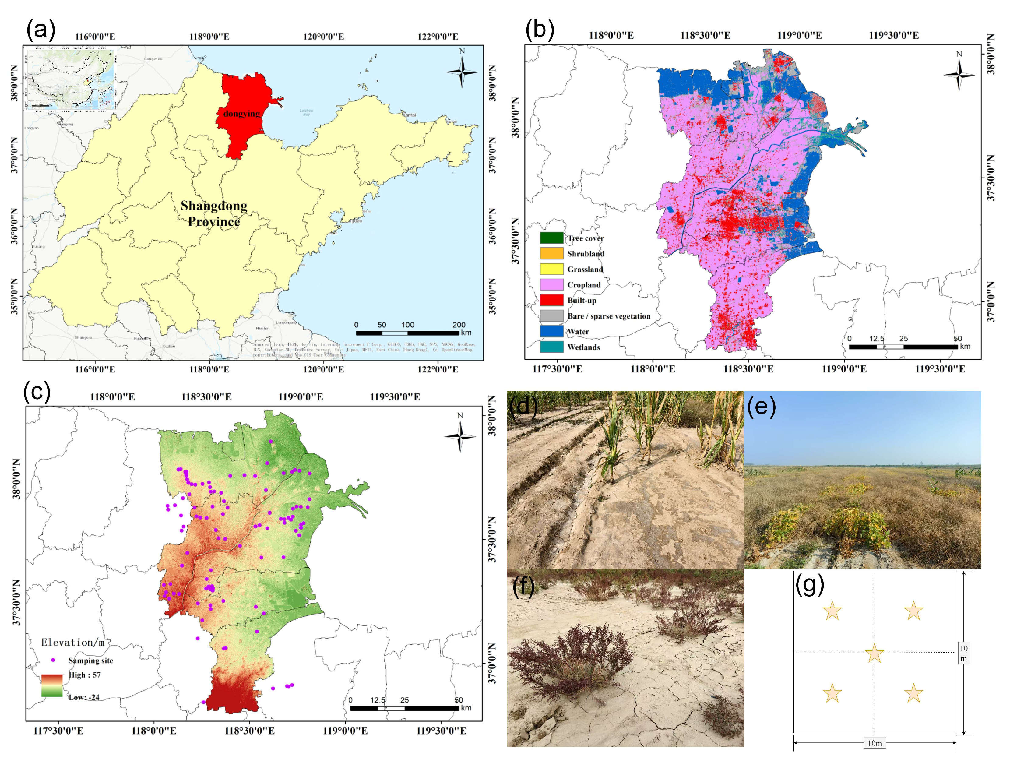
2.1. Study Area

Dongying City is located in the northern part of Shandong Province, China (118°07′–119°10′E, 36°55′–38°10′N), situated at the heart of the Yellow River Delta and adjacent to the Bohai Sea (Figure 1). The terrain is predominantly flat, characterized mainly by the alluvial plains of the Yellow River, and represents a typical coastal wetland geomorphology. The city comprises three districts and two counties, covering a total area of approximately 8,243 square kilometers.

Dongying experiences a warm temperate continental monsoon climate with distinct seasons, an average annual temperature of about 12.3 °C, and annual precipitation ranging from 550 mm to 660 mm. The region is marked by abundant summer rainfall and cold, dry winters. Its proximity to the Bohai Sea and the Yellow River estuary contributes to a relatively humid climate, supporting agricultural development and the formation and preservation of wetland ecosystems.

The primary soil types in Dongying are tidal soils and saline soils. Tidal soils are closely linked to sediment deposition from Yellow River floods, which carry mineral- and nutrient-rich sediments that, over time, develop into fertile soils. Due to the city’s proximity to the ocean, the groundwater table is relatively high, and seawater intrusion leads to elevated soil salinity.

As shown in Figure 1b, the LULC in Dongying includes tree cover, shrubland, grassland, cropland, built-up areas, bare/sparse vegetation, water bodies, and wetlands. The region’s agriculture features diverse crops, including wheat, cotton, soybeans, and corn, cultivated in either two-season or one-season planting systems.

2.2. Field Data Collection

From 10 to 15 October 2024, during a Sentinel-2 satellite overpass of the Yellow River Delta, the research team conducted a comprehensive field landscape survey and soil sample collection. A total of 105 sampling points were systematically established based on variations in soil types, landscape characteristics, cropping patterns, and geomorphological features. Soil samples were collected using a five-point composite sampling method from a depth of 0–20 cm. At each sampling location, global positioning system coordinates were recorded, and representative landscape photographs were taken.

After collection, the samples were transported to the laboratory, air-dried, mechanically ground, and sieved through a 2 mm mesh. A 20 g aliquot of the processed soil was thoroughly mixed with 100 mL of distilled water, producing a soil–water suspension at a mass-to-volume ratio of 1:5 for measuring soil electrical conductivity. Concurrent measurements of soil salinity and pH were also performed.

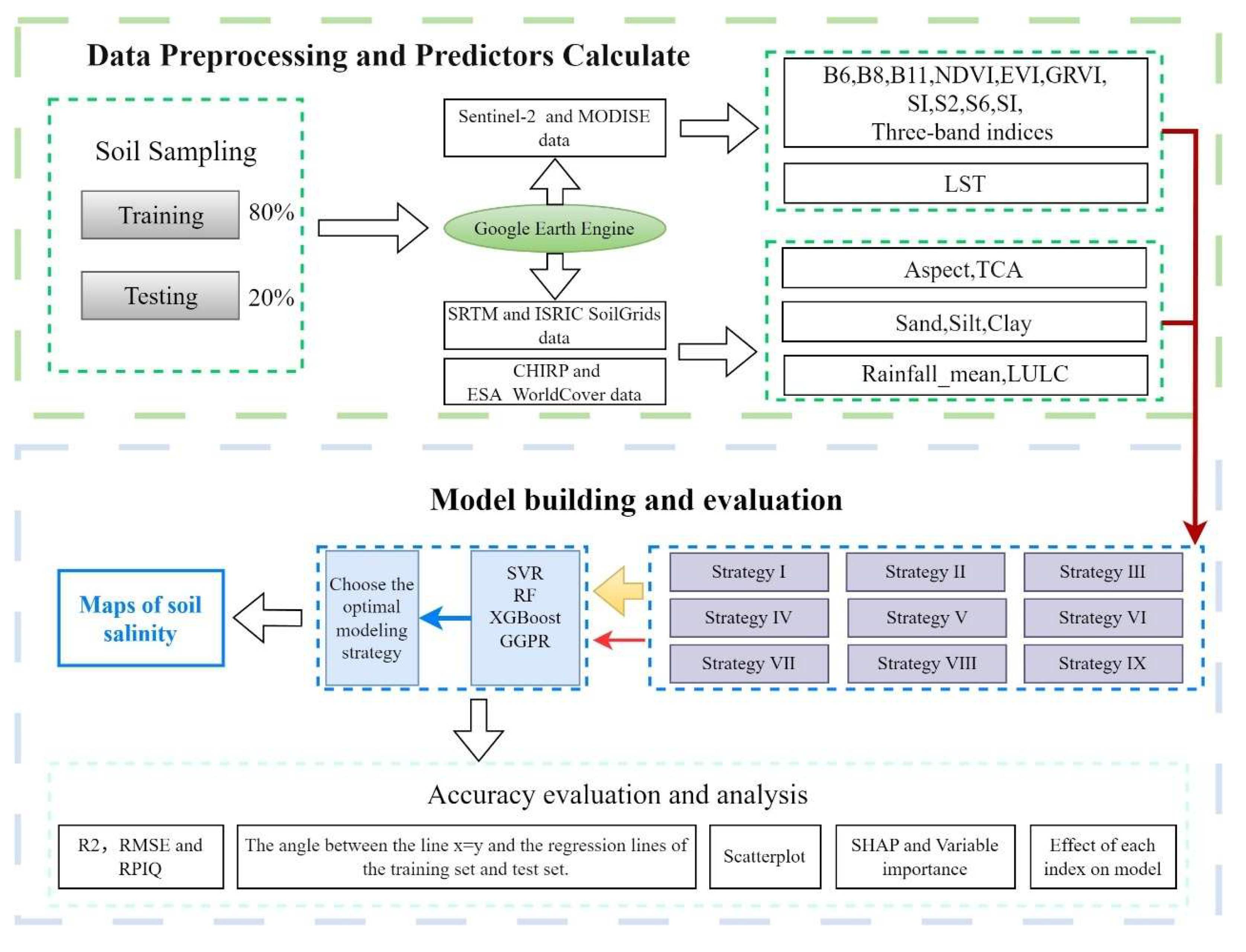
2.3. Satellite Data Selection and Preprocessing

The process of soil salinization and alkalinization involves multiple environmental source variables. This study adopts the SCORPAN framework (S: Soil properties, C: Climate, O: Organisms, R: Relief, P: Parent material, A: Age, N: Spatial location) to select environmental covariates encompassing soil properties, vegetation, topography, climate, LULC, TBI, and Vegetation Type Factors.

To efficiently process large-scale remote sensing data, this research employs the Google Earth Engine (GEE) platform, leveraging its extensive repository of Earth observation data and powerful cloud computing capabilities. All remote sensing environmental variables were derived from the GEE platform, specifically including 10 m resolution Sentinel-2 imagery acquired between October 10 and 15, 2024; MODIS surface reflectance products; ESA WorldCover 2020 LULC data at 10 m resolution; and the SRTM digital elevation model (DEM).

This study employed a systematic approach to data processing. First, field soil samples were collected using a five-point composite sampling method, in which soil from the center and four surrounding points at each sampling location was combined. Each mixed sample represented the average soil properties within a small area and was treated as representative point data corresponding to the center of a 10 m × 10 m satellite pixel when spatially matched.

Second, to ensure the comparability of all environmental covariates at a consistent spatial scale, rigorous resolution standardization was applied to all raster datasets. Using the spatial resampling capabilities of the GEE platform, datasets with resolutions coarser than 10 m were upsampled to a uniform resolution of 10 m using the nearest neighbor method.

From 10 to 15 October 2024, Sentinel-2 imagery with cloud cover below 10% was selected, and cloud pixels were removed using the cloud masking algorithm provided by the GEE platform. Subsequently, a minimum cloud cover composite image for this period was generated using mean compositing. Based on this composite image, a series of spectral indices—including vegetation indices, salinity indices, and TBI—were calculated.

Additionally, surface temperature data for the period from September to November 2024 were derived from MODIS data, which were resampled to a resolution of 10 m. Terrain factors were extracted from the resampled 10 m SRTM DEM. LULC information was obtained directly from the ESA WorldCover 2020 dataset. Furthermore, following the methodology proposed by Guo et al., time series analyses of vegetation indices (VIs) were conducted using Sentinel-2 time series products on the GEE platform, allowing for the derivation of Vegetation Type Factors [36].

Finally, recognizing that soil salinity in urban and water body areas cannot be effectively retrieved via remote sensing, pixels corresponding to these two land use types were identified and excluded using the ESA WorldCover 2020 dataset. This step helped ensure the reliability of the final soil salinization and alkalinization inversion results.

2.4. Environmental Covariate Selection

This study is grounded in the theoretical framework of the SCORPAN model and systematically designs nine variable combination strategies to explore the relative contributions and interactions of different environmental covariates in predicting soil salinity. The core of the strategy design lies in the stepwise introduction and comparison of key variables to evaluate their effects on model predictive performance.

Specifically, Strategy I serves as the baseline model, strictly adhering to the essential components of the SCORPAN framework by incorporating representative soil properties, climatic factors, biological influences, and topographic variables. Building upon Strategy I, Strategy II integrates the original spectral reflectance information from Sentinel-2 imagery to assess the added value of raw spectral data in salinity prediction. Subsequently, Strategies III through IX sequentially or collectively incorporate salinity indices and Vegetation Type Factors. These strategies are meticulously designed to achieve two core objectives. First, they quantify the specific impact of particular indices by measuring the individual contributions of critical variables, such as salinity indices and Vegetation Type Factors, to improving model predictive accuracy. Second, they elucidate the relative importance of these variables, with a focus on comparing the predictive efficacy of salinity indices versus Vegetation Type Factors in forecasting the spatial distribution of soil salinity, thereby identifying which variable offers greater predictive advantage in saline environments.

Together, the nine strategies form an experimental system based on a controlled variable approach, allowing us to isolate the effects of different variable combinations and providing deeper insights into the complex relationships between environmental variables and soil salinity. A detailed composition of the variables included in each strategy is presented in

Table 1. Features corresponding to different strategies (LST: Land Surface Temperature; NDVI: Normalized Difference Vegetation Index; EVI: Enhanced Vegetation Index; GRVI: Green Red Vegetation Index; NDVI_PC1-PC3: Principal components 1–3 of NDVI principal component analysis; NDVI_max: Maximum value of NDVI; EVI_PC1-PC3: Principal components 1–3 of EVI principal component analysis; EVI_max is the maximum value of EVI, TCA is Topographic Contributing Area, LULC is Land Use/Land Cover, TBI5 is the three-band index, B6, B8, and B11 are the Red Edge 2, near-infrared, and short-wave infrared bands of Sentinel-2, and S1, S2, S6, and SI are four salinity indices).

Strategy	Feature
Strategy I	Sand, silt, clay, Rainfall_mean, LST, NDVI, EVI, GRVI, Aspect, TCA, LULC
Strategy II	Sand, silt, clay, Rainfall_mean, LST, NDVI, EVI, GRVI, Aspect, TCA, LULC, TBI5, B6, B8, B11
Strategy III	Sand, silt, clay, Rainfall_mean, LST, NDVI, EVI, GRVI, Aspect, TCA, LULC, TBI5, B6, B8, B11, S1, S2, S6, SI
Strategy IV	Sand, silt, clay, Rainfall_mean, LST, NDVI, EVI, GRVI, Aspect, TCA, LULC, TBI5, B6, B8, B11, NDVI_PC1, NDVI_PC2, NDVI_PC3, NDVI_max
Strategy V	Sand, silt, clay, Rainfall_mean, LST, NDVI, EVI, GRVI, Aspect, TCA, LULC, TBI5, B6, B8, B11, EVI_PC1, EVI_PC2, EVI_PC3, EVI_max
Strategy VI	Sand, silt, clay, Rainfall_mean, LST, NDVI, EVI, GRVI, Aspect, TCA, LULC, TBI5, B6, B8, B11, S1, S2, S6, SI, NDVI_PC1, NDVI_PC2, NDVI_PC3, NDVI_max
Strategy VII	Sand, silt, clay, Rainfall_mean, LST, NDVI, EVI, GRVI, Aspect, TCA, LULC, TBI5, B6, B8, B11, S1, S2, S6, SI, EVI_PC1, EVI_PC2, EVI_PC3, EVI_max
Strategy VIII	Sand, silt, clay, Rainfall_mean, LST, NDVI, EVI, GRVI, Aspect, TCA, LULC, TBI5, B6, B8, B11, NDVI_PC1, NDVI_PC2, NDVI_PC3, NDVI_max, EVI_PC1, EVI_PC2, EVI_PC3, EVI_max
Strategy IX	Sand, silt, clay, Rainfall_mean, LST, NDVI, EVI, GRVI, Aspect, TCA, LULC, TBI5, B6, B8, B11, S1, S2, S6, SI, NDVI_PC1, NDVI_PC2, NDVI_PC3, NDVI_max, EVI_PC1, EVI_PC2, EVI_PC3, EVI_max

.

2.5. Modelling Framework

2.5.1. Support Vector Regression (SVR)

SVR, derived from Support Vector Machines, is a powerful regression technique that constructs a hyperplane in the feature space with strong generalization capabilities. Its core principle involves establishing an ε-insensitive zone around the hyperplane, within which errors are ignored, allowing the model to tolerate small deviations and reduce overfitting. SVR is well-suited for capturing nonlinear relationships through kernel functions, such as the Radial Basis Function and polynomial kernels. During training, only data points that fall outside the ε-insensitive margin—known as support vectors—are used to optimize the model, thereby improving efficiency and sparsity [41]. Owing to its robustness and resistance to overfitting, SVR is particularly effective for small sample sizes and high-dimensional feature spaces.

2.5.2. Random Forest (RF)

RF is an ensemble learning method that improves predictive performance by aggregating the results of multiple decision trees. Each tree is trained on a bootstrap-sampled subset of the training data, and at each node, a random subset of features is selected for splitting [42]. This technique exhibits strong robustness and resistance to noise, making it well-suited for high-dimensional data and complex nonlinear relationships, while effectively reducing the risk of overfitting. Furthermore, Random Forest is largely insensitive to data distribution and scale, contributing to its widespread application. However, its complex model structure can limit interpretability.

2.5.3. Extreme Gradient Boosting (XBGoost)

XGBoost is an efficient implementation of Gradient Boosting that has become widely used in various regression and classification tasks in recent years. This method iteratively trains multiple weak learners, typically CART decision trees, with each iteration focusing on the residuals from the previous round as the learning target, thereby continuously optimizing overall model performance. XGBoost enhances traditional Gradient Boosted Decision Trees by incorporating second-order derivative information, regularization terms, pruning strategies, and mechanisms for handling missing values, which collectively contribute to its superior accuracy and generalization capability [43]. Additionally, this method supports parallel computation, making it well-suited for processing large-scale data. However, its complex model structure and the cumbersome nature of the parameter tuning process can pose challenges.

2.5.4. Geographical Gaussian Process Regression (GGPR)

GGPR is an extension of Gaussian Process Regression developed within the scikit-learn framework, a widely used Python (v3.9) library for machine learning. As a non-parametric regression method, GGPR makes predictions in a probabilistic manner [44]. It offers two primary functionalities, (1) spatial prediction: GGPR employs spatial similarity as a kernel function to calibrate the GPR model, enabling the prediction of observed values at unknown observation points; (2) exploratory spatial data analysis: building on spatial prediction, it incorporates a Matern kernel function with spatial coordinates to facilitate the use of GeoShapley, thus allowing for the exploration of spatial effects and the interpretation of model results [45].

2.6. Feature Importance

To investigate the impact of features on model predictions during training, this study utilizes SHAP (SHapley Additive exPlanations) analysis and feature importance assessment. SHAP is a method that elucidates the predictions of machine learning models by employing the Shapley value concept from game theory [46,47]. It assigns an importance value to each feature of the model, thereby clarifying the prediction process. Positive SHAP values indicate that a feature contributes positively to the model’s predictive accuracy, whereas negative values suggest a detrimental effect.

2.7. Model Evaluation

This study employs the Root Mean Square Error (RMSE), the coefficient of determination (R²), and the Ratio of Performance to Interquartile Distance (RPIQ) to assess the accuracy of predictions and validation of the research. The formulas for these metrics are presented in Equations (1)–(3). To quantify the alignment between predicted and actual values, we introduced the angle formed between the identity line (x = y) and the empirical distributions of the training and test sets. This angle serves as a geometric indicator of model generalization performance, distributional divergence, and systematic prediction bias.

$$RMSE=\sqrt{{\displaystyle \frac{{\sum }_{i=1}^n({\widehat{y}}_i-y_i{)}^2}{n}}}$$

(1)

$$R^2=1-{\displaystyle \frac{{\sum }_{i=1}^n({\widehat{y}}_i-y_i{)}^2}{{\sum }_{i=1}^n(y_i-\overline{y}{)}^2}}$$

(2)

$$RPIQ={\displaystyle \frac{IQR}{RMSE}}$$

(3)

where ${\widehat{y}}_i$ and $y_i$ represent the model estimates and the true values, respectively; $\overline{y}$ denotes the mean of the true values; and n is the number of data points.

2.8. Specific Process Frameworks

Figure 2 illustrates the framework of the methodology employed in this study. Initially, data preprocessing and predictors are calculated. The soil samples were divided into a training set and a testing set with a ratio of 8:2. Subsequently, relevant remote sensing environmental variables were extracted from Sentinel-2, MODIS, SRTM, ESA WorldCover, etc., datasets, followed by necessary preprocessing. The next step involved model building and evaluation. The remote sensing environmental variables were categorized into nine distinct strategies based on the SCORPAN model. Four machine learning models were then utilized for prediction, with the results being evaluated for accuracy. Additionally, SHAP values were applied to assess the influence of each variable on the model. Finally, the optimal model from each strategy was selected to generate the salinity maps.

3. Results

3.1. Descriptive Statistics of Soil Salt

Table 2. Descriptive statistics of soil salinity data (All units are in g/kg.).

Salt Sample Data	Mean	SD	Skewness	Kurtosis	CV	Min	Median	Max
whole data (n = 105)	4.87	8.32	2.34	4.46	1.71	0.4	1.08	36.34

presents the descriptive statistics of soil salinity, which varies from 0.4 to 36.34 g/kg, with a mean of 4.87 g/kg and a median of 1.08 g/kg. The median is significantly lower than the mean, and the skewness of 2.34 indicates a right-skewed distribution, revealing asymmetry in the data. To approximate a normal distribution, a logarithmic transformation was applied. Additionally, the large standard deviation and a coefficient of variation of 1.71 suggest considerable variability in salinity levels across different samples.

Table 3. Descriptive statistics of soil salinity data for different land use types (All units are in g/kg.).

Salt Sample Data		Count	Mean	SD	Skewness	Kurtosis	CV	Min	Median	Max
LULC	Cropland	83	3.02	6.02	3.87	15.70	2.00	0.40	1.02	36.34
	Built-up	2	11.23	6.30	0.00	−2.00	0.56	6.77	11.23	15.68
	Bare/sparse vegetation	19	12.51	12.26	0.50	−1.37	0.98	0.63	7.23	34.72
	Shrubland	1	1.20	-	-	-	-	1.20	1.20	1.20

summarizes soil salinity statistics across different LULC types. Notably, the largest number of sampling points was recorded in Cropland (n = 83), where salinity ranged from 0.40 to 36.34. In areas classified as Bare/sparse vegetation, 19 samples were collected, with salinity values ranging from 0.63 to 34.72. In contrast, only two samples were obtained from Built-up areas and a single sample from the Shrubland.

Figure 3 illustrates the Pearson correlation between the salinity index and various Vegetation Type Factors, using the logarithmically transformed salinity. The diagonal elements display histograms showing the distribution of each variable, while the scatter plots in the lower triangle depict the relationships between pairs of variables, emphasizing the linear associations and distribution of data points. The upper triangle contains the correlation coefficients between the variables, with color intensity indicating the strength of the correlation—darker shades represent higher correlations, with red denoting positive correlations and blue indicating negative correlations. The values within the squares represent the Pearson correlation coefficients, with significance levels indicated: one asterisk for p < 0.05, two asterisks for p < 0.01, and three asterisks for p < 0.001.

From the figure, it is evident that the SI has the highest correlation with S1 and S2, both exhibiting a correlation coefficient of 1. The next highest correlation is between EVI_PC1 and NDVI_max, which has a coefficient of 0.84, and both are statistically significant with three asterisks.

Following the logarithmic transformation of salt, the data distribution approximates a normal distribution. A strong positive correlation exists between NDVI_PC1 and EVI_PC1 with the logarithmically transformed salinity, showing correlation coefficients of 0.5 and 0.45, respectively. In contrast, NDVI_max exhibits a strong negative correlation with the logarithmically transformed salinity, having a coefficient of −0.58, which is also highly significant. Comparatively, S1, S2, and SI show low and non-significant correlations with salinity.

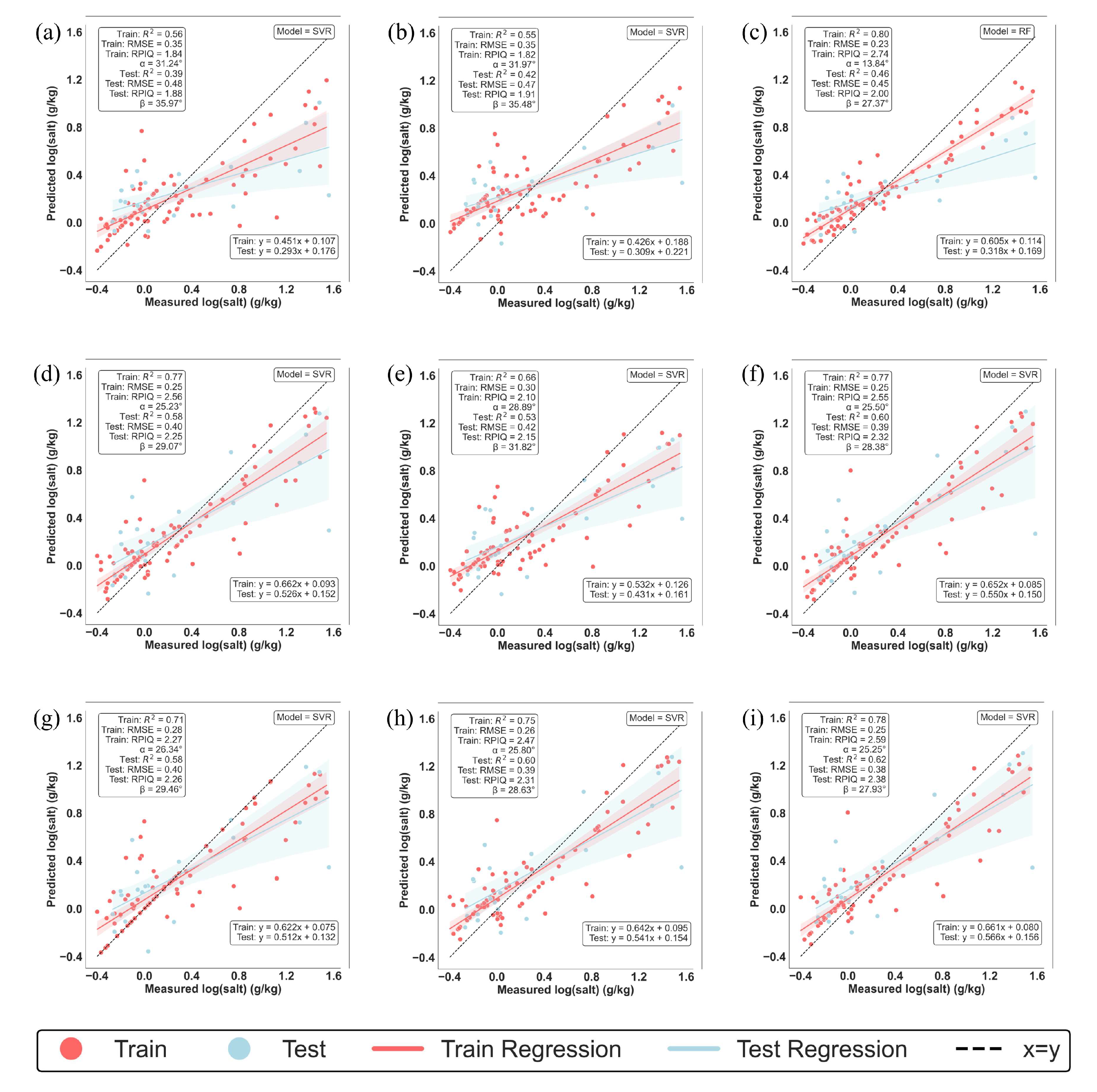
3.2. Comparison of Model Accuracy Under Different Strategies

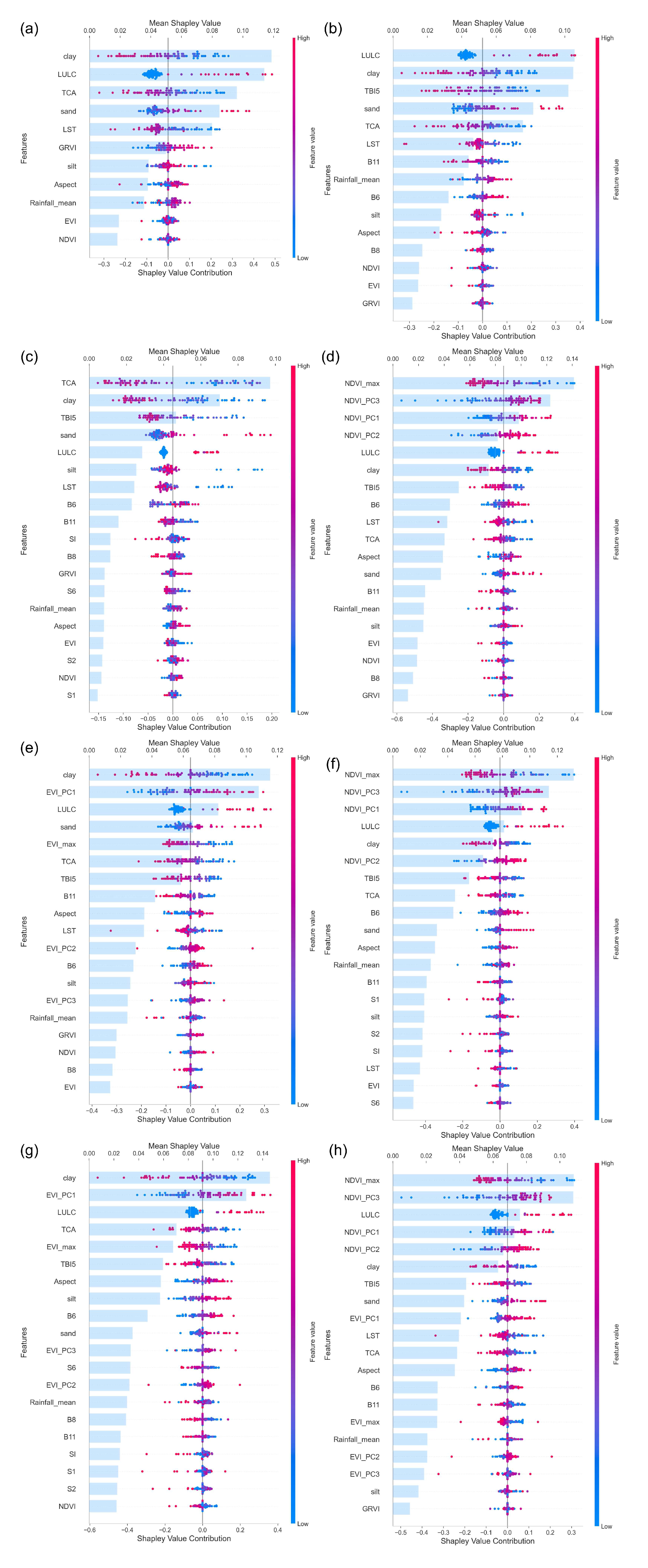
This study employs nine feature combination strategies to model soil salinity prediction using four machine learning algorithms: SVR, RF, XGBoost, and GGPR. Model performance is comprehensively evaluated using the R², RMSE, and RPIQ for both training and testing datasets, as well as the angles (α and β) between the regression lines of the training and testing sets relative to the baseline (y = x). The angles α and β intuitively reflect systematic bias and generalization capability, where smaller deviations indicate greater predictive consistency, while regression lines positioned below y = x suggest underestimation in high-salinity regions.

As illustrated in Figure 4, the SVR model under Strategy IX demonstrates the best overall performance, achieving an R² of 0.62, RMSE of 0.38 g/kg, and RPIQ of 2.38 on the testing set. Although the model exhibits slight systematic underestimation in areas of high salinity (α = 25.25° and β = 27.93°), it maintains strong generalization capability. Closely following, the SVR model under Strategy VIII achieves commendable results, with a testing set R² of 0.60, RMSE of 0.39 g/kg, and RPIQ of 2.31, alongside similarly small deviation angles (α = 25.80° and β = 28.63°), highlighting its stability. Notably, the RF model under Strategy III shows marked overfitting, with an R² of 0.80 on the training set dropping sharply to 0.46 on the testing set (RMSE = 0.45 g/kg, RPIQ = 2.00), underscoring the challenges of using complex models with limited sample sizes.

A systematic comparison across the nine strategies reveals clear patterns. The SVR model consistently outperforms others in most strategies, particularly reflected by the highest testing set R² of 0.62 in Strategy IX. Strategies I and II, which lack sufficient feature combinations, yield weaker performance (testing set R² < 0.42). Despite adding new variables in Strategy III, the overfitting observed in the RF model limits its predictive utility. Strategies IV, V, and VII achieve moderate gains in accuracy (testing set R² > 0.50), while Strategies VI, VIII, and IX combine both high accuracy and robust generalization (testing set R² between 0.60 and 0.62). Considering model accuracy, spatial representation validity, and stability, the SVR model under Strategy IX emerges as the optimal solution for regional salinity mapping.

3.3. SHAP Analysis

Figure 5 presents the feature importance analysis corresponding to the optimal strategy models among the nine strategies, utilizing the SHAP method. SHAP values elucidate the role and directionality of each input feature in the model predictions. The horizontal axis represents the SHAP values, indicating the magnitude of both positive and negative influences of features on prediction outcomes. The color scale reflects the size of the feature values, with blue representing lower values and red indicating higher values. Each point represents an individual sample.

In Figure A1a, the most important features include clay, LULC, TCA, and sand. Notably, high values of clay and TCA negatively impact salinity predictions, while LULC exhibits a positive effect at higher values, indicating that land use and cover types are strong indicators of salinization. In Figure A1b, the newly introduced TBI5 index demonstrates significant feature importance; however, LULC and clay remain dominant in the prediction process. Figure A1c shows that when salinity indices are incorporated into the model, they exhibit lower feature importance, whereas the weight of TCA increases, suggesting that topography’s influence on salinity accumulation becomes significant, leading the model to rely more on topographic and hydrological variables.

Figure A1d reveals that the inclusion of NDVI-type factors results in the highest feature importance for these vegetation-related features, emphasizing their critical role in salinity prediction. Although the EVI-type factor is introduced in Figure A1e, clay retains the highest feature importance, followed by EVI_PC1. Figure A1f,g incorporates salinity indices and various Vegetation Type Factors, respectively. Salinity indices demonstrate low feature importance, while vegetation-type factors indicate significant importance, highlighting the synergistic effects of multidimensional features, including vegetation, hydrology, soil, and meteorological factors.

In Figure 5, all features are included, with NDVI-type factors, LULC, TCA, TBI5, and Aspect identified as the most critical features. Vegetation Type Factors dominate, and the inclusion of topographic factors further enhances the model’s explanatory power. In summary, the key features relied upon by the models differ across various strategies. In models containing vegetation-type factors, these consistently emerge as dominant features, particularly the NDVI-type factors. Soil characteristics (clay, sand, silt) are more important in strategies I–III; however, their relative importance decreases with the enhancement of feature engineering. Topographic and hydrological features are notably critical in strategies III, VI, and IX, while LULC consistently exhibits a high contribution across nearly all strategies, underscoring its foundational role in salinity prediction.

3.4. Soil Salinity Mapping

Figure 6 illustrates the spatial distribution of soil salinity derived from optimal models constructed using nine different strategies. Overall, the spatial distribution trends are consistent across these strategies, with high salinity areas primarily located in the northern and eastern coastal regions of the study area, while low salinity zones are concentrated in the southern and southwestern inland regions. However, notable differences emerge among the strategies regarding salinity gradient expression, peak salinity values, and clarity of patch structures. Specifically, Strategy III predicts a maximum salinity value of 18.78 g/kg, whereas Strategy IV reaches a peak of 37.25 g/kg, indicating a degree of overestimation. In contrast, Strategies V, VII, VIII, and IX exhibit a more balanced spatial transition and clearer boundaries. Notably, Strategies VIII and IX present a coherent and continuous distribution of high salinity areas that align well with the regional topography and geomorphological characteristics. Overall, the inversion maps generated by Strategies VIII and IX—showing soil salinity values ranging from 0.45 to 34.59 g/kg and 0.35 to 32.88 g/kg, respectively—demonstrate the best spatial consistency, numerical rationality, and ecological interpretability, closely reflecting the characteristics observed in the field.

4. Discussion

In this study, we systematically evaluated the performance of nine different strategies for predicting soil salinity, with a focus on both model accuracy and feature contribution. Our objective was to accurately predict soil salinity and generate spatial distribution maps. We began by performing a correlation analysis of the soil salinity data along with several features, revealing potential relationships between these features and soil salinity. Subsequently, we employed four models within the framework of the nine strategies to predict soil salinity, utilizing SHAP values to assess the importance of each feature in the models. This analysis further clarified the contributions and roles of different features in predicting soil salinity. Additionally, we conducted a detailed comparison of feature importance to identify which features are most critical for soil salinity prediction. Finally, we addressed various uncertainties associated with our research findings.

4.1. Comparing the Effects of Different Characteristics on Soil Salinity Mapping

This study systematically compares the salinity prediction performance of four machine learning models across nine feature strategies, revealing that SVR consistently outperforms others in eight of the strategies, followed closely by RF. As shown in Figure 4, models using strategies I and II performed poorly, with test set R² values falling below 0.42, underscoring the limitations of basic feature combinations in characterizing complex saline environments. In contrast, strategies VI and IX demonstrated notable improvements in accuracy due to the integration of Vegetation Type Factors. Notably, the SVR model under strategy IX achieved the highest performance, with an R² of 0.62 on the test set, representing a 48.4% increase compared to strategy I.

This improvement is attributable to the dynamic quantification capability of Vegetation Type Factors in capturing vegetation responses to salt stress. By incorporating time-series metrics derived from NDVI and EVI using high temporal and spatial resolution Sentinel-2 imagery, Vegetation Type Factors effectively detect phenological anomalies in vegetation under saline conditions, such as shortened growing seasons, reduced green peak values, and lower biomass. This approach overcomes the inherent physical limitations of traditional spectral indices in directly detecting soil salinity in vegetated areas [48]. It is also noteworthy that the RF model under strategy III exhibited typical overfitting, with a training set R² as high as 0.80 but dropping to 0.46 on the test set, highlighting the limited generalization capacity of complex models when sample sizes are small.

Integrating SHAP and feature importance analyses (Figure 5 and Figure A1) reveals that in the basic strategies I and II, the models rely heavily on static soil properties and LULC, resulting in limited responsiveness to environmental dynamics. The contribution of the SI introduced in strategy III remains generally below 10%, corroborating its reduced spectral sensitivity in vegetated areas. A pivotal shift occurs in strategies IV and V, where Vegetation Type Factors emerge as primary features and lead to an improvement in model accuracy exceeding 0.15. This marks the transition to predictive dominance driven by indirectly capturing salt stress through the quantification of phenological anomalies in vegetation.

In strategies VI to IX, the importance of Vegetation Type Factors significantly surpasses that of salinity indices. Notably, strategies VIII and IX, which incorporate multidimensional Vegetation Type Factors, show that NDVI-type factors account for over 30% of the SHAP values, effectively characterizing the temporal dynamics of vegetation decline under salt stress. Meanwhile, auxiliary variables such as clay content, LULC, and TCA contribute to a synergistic enhancement network that collectively improves model robustness.

This indicates that Vegetation Type Factors effectively capture the dynamic coupling between soil salinity and vegetation responses. Derived from NDVI/EVI time series, Vegetation Type Factors provide composite metrics that more accurately characterize the cumulative effects of salinity on vegetation growth throughout the growing season, thereby mitigating the influence of sporadic factors that may distort single-time-point data [36,38]. In areas with high salinity, vegetation cover is often suppressed, whereas regions with lower salinity typically exhibit more stable or elevated vegetation indices. Vegetation Type Factors can distinguish these conditions over extended time scales, reducing the model’s tendency to overestimate low-salinity soils and underestimate high-salinity soils [49].

The spatial distribution of soil salinity is shaped by complex factors such as topography, hydrology, and management practices. Vegetation Type Factors can indirectly reflect the long-term impacts of these environmental drivers on salinity distribution [37]. Furthermore, compared to traditional salinity indices that rely on single spectral characteristics, Vegetation Type Factors incorporate richer temporal spectral information, thereby reducing noise caused by variations in surface moisture, agricultural practices, or observational timing. For instance, the results of this study show that although introducing salinity indices improves R² in the training set, their contribution to test set performance remains limited, and their feature importance ranking is low. In contrast, integrating Vegetation Type Factors significantly enhances model performance on the test set, with notably higher feature importance rankings.

From a mechanistic perspective, soil salinity affects vegetation cover by altering soil moisture availability and the physiological and biochemical processes of plants. The use of time series characteristics more effectively captures these nonlinear and lagged responses [38].

In contrast, salinity feature indices perform relatively poorly in areas with dense vegetation cover. For example, Ma et al. applied various spectral indices to construct soil salinity inversion models, but found that these indices did not exhibit significant predictive effectiveness [50]. Similarly, Dong et al. reported that although introducing the CR index substantially improved model accuracy, traditional salinity indices contributed little to the overall performance [51]. These findings suggest that while salinity indices may be effective in bare or sparsely vegetated areas, their predictive capacity declines markedly in regions with dense vegetation.

This evidence further highlights that in areas with dense vegetation or strong soil–vegetation interactions, vegetation-related indices may offer greater predictive advantages than salinity indices. Additionally, auxiliary variables such as clay content, LULC, and TCA have been shown to significantly enhance model performance. For instance, Ma et al. emphasized the role of soil environment and land use type in shaping soil salinity inversion models [50,52]. Shi et al. further noted that separate models may be necessary for different land use types, as these influence soil moisture dynamics, evapotranspiration, and salt accumulation, thereby indirectly affecting salinity distribution. High clay content often indicates poor drainage conditions and a tendency for salt retention, whereas TCA captures the impact of topography on moisture accumulation—both of which are critical for modeling the spatial distribution of soil salinity.

This study demonstrates that Vegetation Type Factors, derived from high temporal and spatial resolution time series, can substantially improve the accuracy of soil salinity inversion, particularly in areas with moderate to high vegetation cover, where they outperform traditional salinity indices. Moreover, incorporating auxiliary variables such as clay content, LULC, and TCA further enhances model stability and generalizability. Collectively, these findings establish a more robust methodological framework for future monitoring of soil salinity in complex landscape regions.

4.2. Uncertainty Analysis of the Current Study

This study employs four machine learning models across nine feature combination strategies to predict and map soil salinity; however, several sources of uncertainty remain. First, the uneven spatial distribution of samples—particularly in critical areas such as the coastal zone and southern Dongying—results in lower sampling density, which constrains local predictive accuracy and limits the detailed characterization of salinity in highly heterogeneous regions. Second, dense vegetation cover interferes with spectral signals, diminishing the effectiveness of traditional SI across much of the study area. In contrast, Vegetation Type Factors demonstrate stronger predictive capabilities, supporting the validity of vegetation physiological responses as indirect indicators of salinity. Third, the reliance on Sentinel-2 data from autumn 2024 to construct Vegetation Type Factors restricts temporal coverage, failing to capture the full annual dynamics of vegetation responses to salt stress. Future research should incorporate multi-seasonal and long-term observations to improve the ecological representativeness of Vegetation Type Factors. Fourth, potential errors in sample collection and laboratory analysis may affect model outcomes. While these errors have limited impact on the overall spatial pattern mapping, they constrain the absolute predictive accuracy.

To address these limitations, future work should focus on optimizing sampling design to increase spatial coverage, alongside implementing standardized quality control procedures to improve data reliability. Additionally, further exploration of feature engineering could help identify spectral and temporal variables more sensitive to salinity stress. Expanding temporal analysis by integrating multi-temporal remote sensing data throughout the year may enable the development of more universally applicable Vegetation Type Factors. Collectively, these improvements could enhance prediction accuracy, providing stronger scientific support for precise saline soil management and sustainable agricultural development.

5. Conclusions

This study systematically evaluates the performance of nine variable combination strategies for soil salinity inversion in typical salinized areas, focusing on model accuracy, feature importance, and spatial distribution rationality. The main conclusions are as follows:

• Model Performance and Selection: Among the evaluated machine learning models, SVR demonstrated the best performance under Strategy IX, which integrates multiple environmental covariates, achieving an R² of 0.62 on the validation set. This significantly outperformed the RF, XGBoost, and GGPR models, highlighting SVR’s effectiveness in capturing complex nonlinear relationships in salinity prediction.
• Contribution of Features: SHAP value analysis and feature importance rankings identified Vegetation Type Factors as the most influential predictor of soil salinity, surpassing the explanatory power of traditional salinity indices in vegetated regions. Other important variables included clay content, LULC, TBI, and TCA, all of which contributed substantially to explaining spatial variations in soil salinity.
• Applicability for Spatial Mapping: Salinity maps generated from strategies incorporating Vegetation Type Factors exhibited superior spatial coherence and natural gradient transitions. These maps demonstrated clear patch boundaries, strong spatial continuity in high-salinity areas, and patterns consistent with regional topography and ecological processes, underscoring the value of Vegetation Type Factors in improving the spatial realism and practical utility of salinity mapping.

By constructing a strategy framework that integrates multi-source remote sensing indices, environmental covariates, and Vegetation Type Factors, this study demonstrates that combining SVR models with vegetation-based and multi-source environmental variables provides an effective paradigm for enhancing regional-scale soil salinity prediction accuracy. The findings offer both a theoretical foundation and actionable methodological guidance for the precise identification, dynamic monitoring, and sustainable management of salinized lands.

References

1. Chi, Y.; Sun, J.; Liu, W.; Wang, J.; Zhao, M. Mapping coastal wetland soil salinity in different seasons using an improved comprehensive land surface factor system. Ecol. Indic. 2019, 107, 105517. [Google Scholar] [CrossRef]
2. Abuelgasim, A.; Ammad, R. Mapping soil salinity in arid and semi-arid regions using Landsat 8 OLI satellite data. Remote Sens. Appl. Soc. Environ. 2019, 13, 415–425. [Google Scholar] [CrossRef]
3. Alkharabsheh, H.M.; Seleiman, M.F.; Hewedy, O.A.; Battaglia, M.L.; Jalal, R.S.; Alhammad, B.A.; Schillaci, C.; Ali, N.; Al-Doss, A. Field Crop Responses and Management Strategies to Mitigate Soil Salinity in Modern Agriculture: A Review. Agronomy 2021, 11, 2299. [Google Scholar] [CrossRef]
4. Ge, X.; Ding, J.; Teng, D.; Wang, J.; Huo, T.; Jin, X.; Wang, J.; He, B.; Han, L. Updated soil salinity with fine spatial resolution and high accuracy: The synergy of Sentinel-2 MSI, environmental covariates and hybrid machine learning approaches. Catena 2022, 212, 106054. [Google Scholar] [CrossRef]
5. Wang, F.; Shi, Z.; Biswas, A.; Yang, S.; Ding, J. Multi-algorithm comparison for predicting soil salinity. Geoderma 2020, 365, 114211. [Google Scholar] [CrossRef]
6. Han, L.; Ding, J.; Ge, X.; He, B.; Wang, J.; Xie, B.; Zhang, Z. Using spatiotemporal fusion algorithms to fill in potentially absent satellite images for calculating soil salinity: A feasibility study. Int. J. Appl. Earth Obs. Geoinf. 2022, 111, 102839. [Google Scholar] [CrossRef]
7. Han, L.; Ding, J.; Zhang, J.; Chen, P.; Wang, J.; Wang, Y.; Wang, J.; Ge, X.; Zhang, Z. Precipitation events determine the spatiotemporal distribution of playa surface salinity in arid regions: Evidence from satellite data fused via the enhanced spatial and temporal adaptive reflectance fusion model. Catena 2021, 206, 105546. [Google Scholar] [CrossRef]
8. Wang, J.; Ding, J.; Yu, D.; Teng, D.; He, B.; Chen, X.; Ge, X.; Zhang, Z.; Wang, Y.; Yang, X.; et al. Machine learning-based detection of soil salinity in an arid desert region, Northwest China: A comparison between Landsat-8 OLI and Sentinel-2 MSI. Sci. Total Environ. 2020, 707, 136092. [Google Scholar] [CrossRef]
9. Wang, J.; Ding, J.; Yu, D.; Ma, X.; Zhang, Z.; Ge, X.; Teng, D.; Li, X.; Liang, J.; Lizaga, I.; et al. Capability of Sentinel-2 MSI data for monitoring and mapping of soil salinity in dry and wet seasons in the Ebinur Lake region, Xinjiang, China. Geoderma 2019, 353, 172–187. [Google Scholar] [CrossRef]
10. Douaoui, A.E.K.; Nicolas, H.; Walter, C. Detecting salinity hazards within a semiarid context by means of combining soil and remote-sensing data. Geoderma 2006, 134, 217–230. [Google Scholar] [CrossRef]
11. Mao, W.; Kang, S.; Wan, Y.; Sun, Y.; Li, X.; Wang, Y. Yellow River Sediment as a Soil Amendment for Amelioration of Saline Land in the Yellow River Delta. Land Degrad. Dev. 2014, 27, 1595–1602. [Google Scholar] [CrossRef]
12. Li, J.; Gong, Y.; Jiang, C. Spatio-temporal differentiation and policy optimization of ecological well-being in the Yellow River Delta high-efficiency eco-economic zone. J. Clean. Prod. 2022, 339, 130717. [Google Scholar] [CrossRef]
13. Zhai, J.; Jin, D.; Chen, Y.; Liu, X.; Yang, X.; Hou, P.; Xu, Y. Ecological changes, problems and countermeasures in the High Efficiency Eco-economic Zone of the Yellow River Delta. Resour. Sci. 2020, 42, 517–526. [Google Scholar] [CrossRef]
14. Xia, J.; Ren, J.; Zhang, S.; Wang, Y.; Fang, Y. Forest and grass composite patterns improve the soil quality in the coastal saline-alkali land of the Yellow River Delta, China. Geoderma 2019, 349, 25–35. [Google Scholar] [CrossRef]
15. Mahajan, S.; Tuteja, N. Cold, salinity and drought stresses: An overview. Arch. Biochem. Biophys. 2005, 444, 139–158. [Google Scholar] [CrossRef] [PubMed]
16. Wang, F.; Yang, S.; Wei, Y.; Shi, Q.; Ding, J. Characterizing soil salinity at multiple depth using electromagnetic induction and remote sensing data with random forests: A case study in Tarim River Basin of southern Xinjiang, China. Sci. Total Environ. 2021, 754, 142030. [Google Scholar] [CrossRef] [PubMed]
17. Hu, J.; Peng, J.; Zhou, Y.; Xu, D.; Zhao, R.; Jiang, Q.; Fu, T.; Wang, F.; Shi, Z. Quantitative Estimation of Soil Salinity Using UAV-Borne Hyperspectral and Satellite Multispectral Images. Remote Sens. 2019, 11, 736. [Google Scholar] [CrossRef]
18. Hassani, A.; Azapagic, A.; Shokri, N. Predicting long-term dynamics of soil salinity and sodicity on a global scale. Proc. Natl. Acad. Sci. USA 2020, 117, 33017–33027. [Google Scholar] [CrossRef]
19. Han, L.; Liu, D.; Cheng, G.; Zhang, G.; Wang, L. Spatial distribution and genesis of salt on the saline playa at Qehan Lake, Inner Mongolia, China. Catena 2019, 177, 22–30. [Google Scholar] [CrossRef]
20. Ding, J.; Yu, D. Monitoring and evaluating spatial variability of soil salinity in dry and wet seasons in the Werigan–Kuqa Oasis, China, using remote sensing and electromagnetic induction instruments. Geoderma 2014, 235–236, 316–322. [Google Scholar] [CrossRef]
21. Scudiero, E.; Skaggs, T.H.; Corwin, D.L. Regional scale soil salinity evaluation using Landsat 7, western San Joaquin Valley, California, USA. Geoderma Reg. 2014, 2–3, 82–90. [Google Scholar] [CrossRef]
22. Gorji, T.; Sertel, E.; Tanik, A. Monitoring soil salinity via remote sensing technology under data scarce conditions: A case study from Turkey. Ecol. Indic. 2017, 74, 384–391. [Google Scholar] [CrossRef]
23. Butcher, K.; Wick, A.F.; DeSutter, T.; Chatterjee, A.; Harmon, J. Soil Salinity: A Threat to Global Food Security. Agron. J. 2016, 108, 2189–2200. [Google Scholar] [CrossRef]
24. Targulian, V.O.; Krasilnikov, P.V. Soil system and pedogenic processes: Self-organization, time scales, and environmental significance. Catena 2007, 71, 373–381. [Google Scholar] [CrossRef]
25. Farifteh, J.; Van der Meer, F.; Atzberger, C.; Carranza, E.J.M. Quantitative analysis of salt-affected soil reflectance spectra: A comparison of two adaptive methods (PLSR and ANN). Remote Sens. Environ. 2007, 110, 59–78. [Google Scholar] [CrossRef]
26. Yahiaoui, I.; Douaoui, A.; Zhang, Q.; Ziane, A. Soil salinity prediction in the Lower Cheliff plain (Algeria) based on remote sensing and topographic feature analysis. J. Arid Land 2015, 7, 794–805. [Google Scholar] [CrossRef]
27. Khan, N.M.; Rastoskuev, V.V.; Sato, Y.; Shiozawa, S. Assessment of hydrosaline land degradation by using a simple approach of remote sensing indicators. Agric. Water Manag. 2005, 77, 96–109. [Google Scholar] [CrossRef]
28. Habibi, V.; Ahmadi, H.; Jafari, M.; Moeini, A. Mapping soil salinity using a combined spectral and topographical indices with artificial neural network. PLoS ONE 2021, 16, e0228494. [Google Scholar] [CrossRef]
29. Navarro-Pedreño, J.; Jordan, M.M.; Meléndez-Pastor, I.; Gómez, I.; Juan, P.; Mateu, J. Estimation of soil salinity in semi-arid land using a geostatistical model. Land Degrad. Dev. 2007, 18, 339–353. [Google Scholar] [CrossRef]
30. Peng, J.; Biswas, A.; Jiang, Q.; Zhao, R.; Hu, J.; Hu, B.; Shi, Z. Estimating soil salinity from remote sensing and terrain data in southern Xinjiang Province, China. Geoderma 2019, 337, 1309–1319. [Google Scholar] [CrossRef]
31. Zhu, A.X.; Hudson, B.; Burt, J.; Lubich, K.; Simonson, D. Soil Mapping Using GIS, Expert Knowledge, and Fuzzy Logic. Soil Sci. Soc. Am. J. 2001, 65, 1463–1472. [Google Scholar] [CrossRef]
32. Metternicht, G.I.; Zinck, J.A. Remote sensing of soil salinity: Potentials and constraints. Remote Sens. Environ. 2003, 85, 1–20. [Google Scholar] [CrossRef]
33. Zhang, H.; Fu, X.; Zhang, Y.; Qi, Z.; Zhang, H.; Xu, Z. Mapping Multi-Depth Soil Salinity Using Remote Sensing-Enabled Machine Learning in the Yellow River Delta, China. Remote Sens. 2023, 15, 5640. [Google Scholar] [CrossRef]
34. Zhang, T.-T.; Qi, J.-G.; Gao, Y.; Ouyang, Z.-T.; Zeng, S.-L.; Zhao, B. Detecting soil salinity with MODIS time series VI data. Ecol. Indic. 2015, 52, 480–489. [Google Scholar] [CrossRef]
35. Wang, Z.; Zhao, G.; Gao, M.; Chang, C. Spatial variability of soil salinity in coastal saline soil at different scales in the Yellow River Delta, China. Environ. Monit. Assess. 2017, 189, 80. [Google Scholar] [CrossRef] [PubMed]
36. Guo, B.; Yang, X.; Yang, M.; Sun, D.; Zhu, W.; Zhu, D.; Wang, J. Mapping soil salinity using a combination of vegetation index time series and single-temporal remote sensing images in the Yellow River Delta, China. Catena 2023, 231, 107313. [Google Scholar] [CrossRef]
37. Zhang, J.; Zhang, Z.; Chen, J.; Chen, H.; Jin, J.; Han, J.; Wang, X.; Song, Z.; Wei, G. Estimating soil salinity with different fractional vegetation cover using remote sensing. Land Degrad. Dev. 2020, 32, 597–612. [Google Scholar] [CrossRef]
38. Liu, H.; Guo, B.; Yang, X.; Zhao, J.; Li, M.; Huo, Y.; Wang, J. High spatiotemporal resolution vegetation index time series can facilitate enhanced remote sensing monitoring of soil salinization. Plant Soil. 2024, 510, 305–327. [Google Scholar] [CrossRef]
39. Chen, S.; Liang, Z.; Webster, R.; Zhang, G.; Zhou, Y.; Teng, H.; Hu, B.; Arrouays, D.; Shi, Z. A high-resolution map of soil pH in China made by hybrid modelling of sparse soil data and environmental covariates and its implications for pollution. Sci. Total Environ. 2019, 655, 273–283. [Google Scholar] [CrossRef]
40. Malone, B.P.; Minasny, B.; Odgers, N.P.; McBratney, A.B. Using model averaging to combine soil property rasters from legacy soil maps and from point data. Geoderma 2014, 232–234, 34–44. [Google Scholar] [CrossRef]
41. Smola, A.J.; Schölkopf, B. A tutorial on support vector regression. Stat. Comput. 2004, 14, 199–222. [Google Scholar] [CrossRef]
42. Breiman, L. Random forests. Mach. Learn. 2001, 45, 5–32. [Google Scholar] [CrossRef]
43. Chen, T.; Guestrin, C. XGBoost: A scalable tree boosting system. In Proceedings of the KDD ‘16: The 22nd ACM SIGKDD International Conference on Knowledge Discovery and Data Mining, San Francisco, CA, USA, 13 August 2016; pp. 785–794. [Google Scholar]
44. Wang, J.; Filippi, P.; Haan, S.; Pozza, L.; Whelan, B.; Bishop, T.F.A. Gaussian process regression for three-dimensional soil mapping over multiple spatial supports. Geoderma 2024, 446, 116899. [Google Scholar] [CrossRef]
45. Jiao, Z.; Tao, R. Geographical Gaussian Process Regression: A Spatial Machine-Learning Model Based on Spatial Similarity. Geogr. Anal. 2025, 57, 507–520. [Google Scholar] [CrossRef]
46. Li, X.; Wang, H.; Qin, S.; Lin, L.; Wang, X.; Cornelis, W. Evaluating ensemble learning in developing pedotransfer functions to predict soil hydraulic properties. J. Hydrol. 2024, 640, 131658. [Google Scholar] [CrossRef]
47. Lundberg, S.M.; Lee, S.-I. A unified approach to interpreting model predictions. Adv. Neural Inf. Process. Syst. 2017, 30, 4765–4774. [Google Scholar]
48. Chakraborty, T.C.; Lee, X.; Ermida, S.; Zhan, W. On the land emissivity assumption and Landsat-derived surface urban heat islands: A global analysis. Remote Sens. Environ. 2021, 265, 112682. [Google Scholar] [CrossRef]
49. Guo, B.; Han, B.; Yang, F.; Fan, Y.; Jiang, L.; Chen, S.; Yang, W.; Gong, R.; Liang, T. Salinization information extraction model based on VI–SI feature space combinations in the Yellow River Delta based on Landsat 8 OLI image. Geomat. Nat. Hazards Risk 2019, 10, 1863–1878. [Google Scholar] [CrossRef]
50. Ma, H.; Zhao, W.; Duan, W.; Ma, F.; Li, C.; Li, Z. Inversion model of soil salinity in alfalfa covered farmland based on sensitive variable selection and machine learning algorithms. PeerJ 2024, 12, e18186. [Google Scholar] [CrossRef]
51. Dong, X.; Li, X.; Zheng, X.; Jiang, T.; Li, X. Effect of Saline Soil Cracks on Satellite Spectral Inversion Electrical Conductivity. Remote Sens. 2020, 12, 3392. [Google Scholar] [CrossRef]
52. Ma, G.; Ding, J.; Han, L.; Zhang, Z.; Ran, S. Digital mapping of soil salinization based on Sentinel-1 and Sentinel-2 data combined with machine learning algorithms. Reg. Sustain. 2021, 2, 177–188. [Google Scholar] [CrossRef]
Figure 1. Sampling locations and positions in Dongying city. (a) Dongying’s location in Shandong Province. (b) Land cover types in Dongying city. (c) Sampling locations and elevations in the Dongying city region. (df) landscape photos of sampling points. (g) Sampling plots.
Remotesensing 17 02619 g001
Figure 2. Flowchart of this study.
Remotesensing 17 02619 g002
Figure 3. Correlation analysis heatmap and data statistics. Significance levels are indicated by asterisks: *, ** and *** marked correlation significant at p ≤ 0.05, p ≤ 0.01 and p ≤ 0.001 level respectively.
Remotesensing 17 02619 g003
Figure 4. Prediction performance of the optimal models under different strategies on the training and testing sets. Figures (ai) represent strategies I–IX, respectively.
Remotesensing 17 02619 g004
Figure 5. SHAP feature importance analysis results of the optimal strategy model.
Remotesensing 17 02619 g005
Figure 6. Spatial distribution map of soil salinity derived from the optimal models under different strategies. Figures (ai) represent strategies I–IX, respectively.
Remotesensing 17 02619 g006