Abstract
The rapid expansion of urban areas necessitates effective monitoring systems for sustainable development planning. Time-series change detection algorithms applied to satellite imagery offer promising solutions, but their comparative effectiveness specifically for urban land cover monitoring remains poorly understood. This study aims to systematically evaluate and optimize three widely used algorithms—LandTrendr, CCDC, and BFAST—selected for their proven capabilities in different land cover change contexts and distinct algorithmic approaches. Using Landsat 5/7/8 (TM/ETM+/OLI) time-series data from 2000 to 2020 and a globally distributed dataset of 200 sample locations spanning six continents, we assess these algorithms across multiple spectral bands and parameter settings for land cover change detection in urban areas. Our analysis reveals that CCDC achieves the highest accuracy (78.14% F1 score) when utilizing complete spectral information (bands B1–B7), outperforming both BFAST (74.32% F1 score with NDVI) and LandTrendr (71.29% F1 score with B1). We demonstrated that, contrary to conventional approaches that prioritize vegetation indices, visible light bands—particularly B1 and B2—achieve higher performance across multiple algorithms. For instance, in LandTrendr, B1 yielded an F1 score of 71.29%, whereas NDVI and EVI produced 56.19% and 53.16%, respectively. Similarly, in CCDC, B2 achieved an F1 score of 72.19%, while NDVI and EVI resulted in 68.57% and 65.33%, respectively. Our findings underscore that parameter optimization and band selection significantly impact detection accuracy, with variations up to 30% observed across different configurations. This comprehensive evaluation provides critical methodological guidance for satellite-based urban expansion monitoring and identifies specific optimization strategies to enhance the application of existing algorithms for urban land cover change detection.
1. Introduction
Global population is rapidly increasing, with especially rapid growth in developing regions where urban populations have surpassed rural populations [1,2,3]. This demographic shift correlates strongly with urban expansion as cities grow to accommodate burgeoning populations [1,4,5,6].
Numerous studies have documented how urban expansion increases environmental and socioeconomic vulnerabilities. The conversion of agricultural to urbanized land uses threatens food production systems [7,8,9], intensifying food security challenges, particularly in developing nations [10]. Climate impacts are also significant, with research establishing clear correlations between urbanization and alterations in extreme temperature events and precipitation patterns [11]. Urban development contributes to heat island intensification [11,12,13,14] and decreases diurnal temperature ranges [15,16], further modifying local and regional climate conditions. Beyond environmental consequences, the urbanization processes exacerbate economic disparities between urban and rural regions while substantially increasing carbon emissions [17]. The breadth and severity of these impacts underscore the critical importance of systematic urban expansion monitoring to support evidence-based urban planning that can effectively mitigate these multifaceted risks.
However, visual inspection and on-site survey methods are expensive and time-consuming, making them impractical for large-scale monitoring. Therefore, satellite imagery, which provides freely available long-term data, has gained significant attention. Models designed to detect land cover changes using time-series satellite imagery have proven to be effective for urban monitoring. The Landsat program, managed jointly by NASA and the U.S. Geological Survey (USGS), represents one of the most valuable Earth observation resources for monitoring environmental change [18]. This continuous record of Earth’s surface began in 1972 and maintains a 16-day observation cycle. Key missions including Landsat 5 (1984–2013) with its Thematic Mapper (TM), Landsat 7 (1999–2024) with the Enhanced Thematic Mapper Plus (ETM+), and Landsat 8 (2013–present) with the Operational Land Imager (OLI) provide consistent 30-m spatial resolution across multiple spectral bands (visible, near-infrared, and mid-infrared) [19,20,21], creating an invaluable, freely accessible archive for analyzing long-term land cover dynamics.
Conventionally, pixel-based spatially explicit land cover classification has been applied to satellite images over time to detect urban expansion by comparing multiple time-series Land Use and Land Cover (LULC) maps [22,23,24,25,26,27,28]. However, these approaches, which create LULC maps at different time steps and then compare them, make it challenging to detect urban expansion accurately, as land cover changes are often confused with misclassification errors that occur over time. LULC maps are not 100% accurate, meaning that some pixels are incorrectly classified. This makes it difficult to distinguish between actual land cover changes and misclassifications when comparing maps from different periods [29].
In response to these challenges, pixel-wise time-series algorithms have been developed to detect change points (e.g., years of change) from time-series satellite images for land cover change detection. Major methods include Landsat-based detection of Trends in Disturbance and Recovery (LandTrendr), Continuous Change Detection and Classification (CCDC), and Breaks for Additive Seasonal and Trend (BFAST) algorithms [30,31,32]. LandTrendr is a model that flexibly captures both abrupt changes and long-term trends from univariate annual composite Landsat time series [30]. CCDC uses multivariate Landsat time-series data and represents seasonal and trend components, as well as abrupt changes, using a linear harmonic model with sine and cosine functions [31]. This model was designed to detect various land cover changes. BFAST decomposes univariate time-series data into trend, seasonal, and residual components using Seasonal and Trend decomposition using Loess (STL), and identifies change points in both seasonal and trend components [32]. These algorithms have been widely applied across diverse land cover change contexts, including urban expansion [33,34,35,36,37], forest loss and vegetation disturbances [38,39,40,41,42,43,44,45,46,47], hydrological changes [48,49,50,51,52,53], and open-pit mining activities with subsequent land restoration [54,55,56,57,58,59]. Several studies have evaluated the detection accuracy of these approaches [44,60,61]. For example, Yan et al. (2021) utilized LandTrendr to monitor urban expansion in Karachi, Pakistan, and achieved an accuracy of 83.76% [33]. Yan et al. (2022) compared the accuracy of LandTrendr, CCDC, and BFAST in detecting forest fires, finding that LandTrendr detected forest fires with 73.4% accuracy, CCDC with 72.0%, and BFAST with 96.2% [60].
Despite these advances, critical research gaps remain in applying these models for urban expansion detection. First, remotely sensed time-series data fluctuations vary substantially across different land cover types and change patterns, suggesting that detection accuracy for urban expansion likely differs from other land cover transitions such as forest disturbance or water body changes. Second, most studies employ default or fixed-parameter settings [33,34,40,41,42,43,44,45,46,47,49,52,53,58,59], despite Kennedy et al. (2010) demonstrating that detection accuracy varies significantly with different parameter combinations [30]. In studies on urban land cover change detection, vegetation indices are often prioritized as they expect a decrease in vegetation activity due to the land cover change [35,36,37]. Systematic evaluations of optimal parameter configurations specifically for urban land cover change detection remain notably absent in the literature. Third, the selection of appropriate spectral bands and indices represents another critical yet underexplored factor affecting detection performance. Landsat satellites capture a wide range of wavelengths—including visible, near-infrared, and shortwave infrared—that enable time-series analysis. While various studies have examined different indices and band combinations for urban land cover changes [62,63,64,65,66], these studies did not consider time-series change-point detection models. Research remains limited in systematically identifying which spectral inputs most effectively detect urban expansion when applied to algorithms such as LandTrendr, CCDC, and BFAST. Lastly, none of the previous studies examined the effect of parameters and band selections for time-series change-point detection models in urban land cover change detection across various conditions at a global scale. Reba and Seto (2020) noted that most existing studies on urban land change monitoring are restricted to individual cities, thereby limiting the generalizability of their conclusions [67]. The spatial and environmental variability of urban land cover change studies underscores the importance of conducting systematic evaluations under standardized modeling conditions using geographically diverse samples.
To address these gaps, this study evaluated the accuracy of the time-series change-point detection methods of LandTrendr, CCDC, and BFAST, using Landsat time-series images for urban expansion monitoring. By collecting data from various regions worldwide and systematically evaluating different parameter settings and spectral inputs, this study developed an approach to determine optimal parameter settings for urban expansion. This approach enhances the accuracy and applicability of urban expansion monitoring and contributes to effective urban planning strategies for sustainable growth.
2. Materials and Methods
Figure 1 shows an overview of the general workflow followed in this study. The critical procedures will be introduced in the following sections in detail.
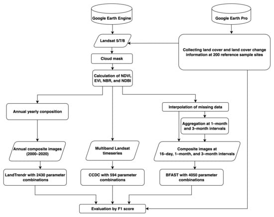
Figure 1.
Flowchart of this study.
2.1. Reference Data Collection
We collected a reference sample dataset using historical, very high-resolution satellite image time series from Google Earth Pro that matched the pixel size of the Landsat imagery [68]. We initially established equal sample sizes for two categories: areas transitioning from non-urban to urban at the urban fringe, and non-urban regions showing no change. After removing unavailable sampling data, we analyzed 200 areas in total: 101 areas where land cover transitioned from non-urban to urban at the urban periphery, and 99 areas where no changes occurred in non-urban regions across the globe. Land cover was documented through visual inspection of historical high-resolution satellite time series in Google Earth Pro, with the year and location of land cover changes recorded annually.
We classified land cover into six categories: Urban, Grassland, Farmland, Forest, Bare land, and Water. Urban refers to artificial, impervious surfaces including buildings, roads, and other concrete or asphalt structures. Grassland consists of open areas dominated by herbaceous vegetation with minimal tree cover. Farmland includes croplands and agricultural fields under active cultivation. Forest describes areas primarily covered by trees with a closed or nearly closed canopy. Bare land comprises exposed soil, rock, or sand with sparse vegetation, while Water includes permanent surface water bodies such as rivers, lakes, and coastal waters. Determining dates of urbanized land cover changes through Google Earth Pro required frequent observations of historical imagery. Image availability varied across regions despite our efforts to minimize geographic bias. Rapidly expanding Asian cities provided abundant imagery and study sites, while Africa and South America had limited suitable imagery, resulting in fewer sites in these regions. Our site selection, therefore, mainly focused on developing countries experiencing rapid population-driven urban expansion. The study sites spanned the globe (Figure 2): 92 in Asia, 38 in Africa, 18 in Europe, 16 in North America, 29 in South America, and 7 in Oceania. Among our 200 reference sample areas, we documented these land cover transitions to urban areas: 49 from Grassland, 30 from Farmland, 13 from Forest, and 9 from Bare land. The unchanged sites included 29 Urban, 26 Farmland, 23 Grassland, 16 Forest, 4 Bare land, and 1 Water.
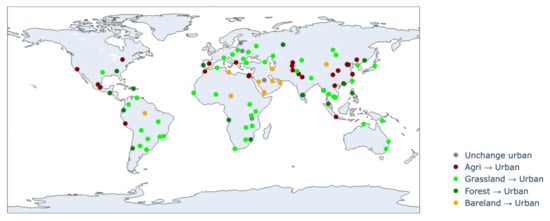
Figure 2.
Distribution of study sites.
2.2. Landsat
Time-series sequences for each study site were obtained from Landsat TM/ETM+/OLI (5, 7, 8) image data archived on the Google Earth Engine (GEE) cloud platform from 2000 to 2020 [69]. Figure 3 shows the time-series data for a point that changed from a grassland to an urban area as an example. Landsat Surface Reflectance (SR) data corrected for atmospheric effects were used. The spatial resolution of Landsat TM/ETM+/OLI images is 30 m, and each pixel contains information corresponding to various bands (data from different wavelength ranges), as well as Quality Assessment (QA) information, which identifies clouds, shadows, snow, and other noise.
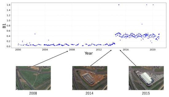
Figure 3.
Example of Landsat B1 time-series. The three images were obtained from Google Earth, showing the land cover change from grassland to urban.
The sequences collected on the GEE were processed using QA masks to replace pixel values with missing values over clouds, shadows, and snow, thus allowing for a clearer reflection of surface conditions. The bands handled in this study consisted of seven bands: B1 (blue, 450–515 nm), B2 (green, 525–600 nm), B3 (red, 630–680 nm), B4 (near-infrared, 845–885 nm), B5 (shortwave infrared1, 1560–1660 nm), and B7 (shortwave infrared2, 2100–2300 nm). In this study, data from Landsat 5, 7, and 8 were used; however, it is important to note that the band configurations differed slightly among these sensors. While Landsat 5 and 7 include B1 (450–515 nm), corresponding to the blue wavelength, Landsat 8 introduced a new coastal aerosol band, Band 1, shifting what was traditionally considered “B1” to B2. Therefore, for consistency across datasets, this study utilized comparable bands starting from B2 (blue, 450–515 nm) for Landsat 8.
In addition to the SR wavelengths, several indices representing vegetation and urban conditions were included in the study: the Normalized Difference Vegetation Index (NDVI), which indicates vegetation distribution and activity (Equation (1)) [70]; the Enhanced Vegetation Index (EVI), which indicates vegetation conditions but is designed to minimize atmospheric influences (Equation (2)); the Normalized Burn Ratio (NBR), often used to indicate vegetation health and the degree of fire damage (Equation (3)); and the Normalized Difference Built-up Index (NDBI), used to identify urbanized areas (Equation (4)) [71].
2.3. Models
2.3.1. LandTrendr
The LandTrendr algorithm captures both abrupt land cover changes and gradual trends using annual time-series Landsat images (Figure 4) [30]. It divides the input time-series data into multiple straight-line segments that represent land-cover states through the connected segments. Potential vertices (years of land cover change) were calculated using deviations from a linear regression line on the time-series data. When excess vertices were identified, those with small change angles were removed, and the segments were connected through all remaining vertices. The p-value of the F-statistic measures the fit between the input time-series data and the fitted segments. This process is repeated for multiple segment numbers, from 1 to the number specified by the maxSegments parameter, to determine the best-fitting model. Several parameters can be adjusted during this process to prevent overfitting and more accurately represent land cover conditions.
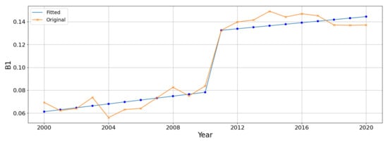
Figure 4.
Example of LandTrendr application.
In this study, the Landsat time-series sequence was averaged annually after removing cloud noise, resulting in a time-series dataset of 21 annual observations from 2000 to 2020, which served as the input for LandTrendr. The evaluated parameters are presented in Table 1. We assessed 2430 parameter combinations derived from 243 combinations of five parameter values and 10 input bands/indices for accuracy.

Table 1.
Parameters to be evaluated in LandTrendr.
2.3.2. CCDC
The CCDC algorithm creates a linear harmonic model that incorporates sine and cosine curves using all available Landsat time series (Figure 5) [31]. Land cover changes are detected by representing seasonal components, trend components, and abrupt changes in the time-series data. The primary processing flow of the CCDC begins with the removal of clouds, shadows, and snow noise using bands 2 and 5. Based on the 12 cloud-free observations in the input time-series data, a fitting model (Equation (5)) was initialized using the ordinary least squares (OLS) method. If the difference between the predicted and observed values exceeded the threshold for the number of times specified by the minObservations parameter, a change was detected.
where each variable and parameter is as follows:
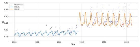
Figure 5.
Example of CCDC application.
- x: Julian day
- i: the i-th Landsat band
- T: Number of days per year (=365)
- : Coefficient for the overall value of the i-th Landsat band
- : Coefficients for intra-annual variability of the i-th Landsat band
- : Coefficient for annual variability of the i-th Landsat band
- : k-th breakpoint
- : Predicted value of the i-th Landsat band on Julian day
The Landsat time-series sequence created on GEE was used directly as the input. The bands/indices tested in the CCDC include B1, B2, B3, B4, B5, B7, NDVI, EVI, NBR, NDBI, and the combination of [B1–B7], for a total of 11 types. The evaluated parameters are listed in Table 2. A total of 594 parameter combinations derived from 54 combinations of four parameter values and 11 input bands/indices were evaluated for accuracy.
Table 2.
Parameters to be evaluated in CCDC.
2.3.3. BFAST
BFAST uses STL decomposition and the moving sum of ordinary least squares (OLS_MOSUM) method to detect changes in the seasonal or trend components of univariate time-series data (Figure 6) [32]. STL decomposes time-series data into three components: trend, seasonal, and residual, as shown in Equation (6). OLS_MOSUM calculates the moving sum of OLS estimates for a specific data interval and evaluates whether this sum shows a statistically significant change. The main processing flow of BFAST begins with decomposing the input univariate time-series data into trend, seasonal, and residual components using STL decomposition. The algorithm then calculates the cumulative difference over time between the trend component () and the regression line using OLS_MOSUM. Breakpoints (identified as land cover changes) were detected when the cumulative sum exceeded the threshold.
where:
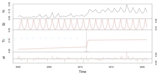
Figure 6.
Example of BFAST application.
- t: Time
- : Observed value at time t
- : Trend component at time t
- : Seasonal component at time t
- : Residual component at time t
BFAST performs optimally with time-series data that exhibit seasonality. In this study, we used Landsat time-series data collected at 16-day intervals. After applying a QA mask, we used the function [72] to interpolate missing values using linear interpolation for non-seasonal data and STL decomposition for seasonal data. We then calculated the 1-month and 3-month average values over specific periods to test the detection performance at different time frequencies.
We selected 10 input bands: B1, B2, B3, B4, B5, B7, NDVI, EVI, NBR, and NDBI. The evaluated parameters are presented in Table 3. We assessed the accuracy across 4050 parameter combinations derived from 135 combinations of four parameter values, 10 input bands, and three time-series data types.
Table 3.
Parameters to be evaluated in BFAST.
2.4. Performance Evaluation and Comparison
In this study, we defined the ’year of urbanization’ as the year of construction completion. While selecting study sites in Google Earth Pro, we observed that land preparation activities like grading and site clearing typically began one to two years before building completion. Therefore, we established a two-year buffer period before the completion date. For performance evaluation, we considered model-detected changes within this buffer window as correct identifications. For example, if a building was completed in 2015, the period of urban land cover change was set to 2013–2015 (see Figure 3). If the model-predicted year of change matched the actual period of urban land cover change (within −2 to 0 years), it was considered as being correctly detected (True Positive, TP). If the model failed to detect the change, it was considered a False Negative (FN). If the model predicted a change at a non-changing point, it was considered a False Positive (FP); if no change was predicted at a non-changing point, it was considered a True Negative (TN). A confusion matrix was then created (Table 4), where , , , and represent the numbers of samples classified as TP, FN, FP, and TN, respectively.
Table 4.
Confusion matrix for change detection results.
Precision, Recall, and F1 score were calculated based on the confusion matrix to evaluate accuracy. Precision represents the proportion of correctly predicted changes among all changes predicted by the model (Equation (7)), whereas recall represents the proportion of correctly predicted changes among all actual changes (Equation (8)). Generally, increasing one metric decreases the other metric. The F1 score, which is the harmonic mean of Precision and Recall, is high only when both metrics are high, making it an effective evaluation measure that balances the two (Equation (9)). In addition, it is appropriate to evaluate models with class imbalances. Therefore, we used the F1 score as the primary evaluation metric in this study.
3. Results
3.1. Model Comparison
We tested 2430 parameter combinations for the LandTrendr, 594 for the CCDC, and 4050 for the BFAST. Table 5 lists the highest F1 scores achieved for each input band and index for the three models. The “Average” row at the bottom represents the mean of the maximum F1 scores across all bands. LandTrendr achieved its highest F1 score (71.29%) using B1 as the input, followed by B2 (66.39%). The model exhibited lower F1 scores when B4, EVI, NBR, and NDBI were used. CCDC achieved the highest F1 score (78.14%) across all tested combinations when using bands B1–B7 together. Using individual bands, the CCDC scored 75.89% for B3 and 72.19% for B2. Similar to LandTrendr, CCDC showed a lower performance with B4, EVI, NBR, and NDBI inputs. BFAST performed best with the NDVI input, achieving a 74.32% F1 score, followed by 72.07% with B7, and 67.35% with EVI. Similar to other models, BFAST showed lower F1 scores when B4, NBR, and NDBI were used. All three models performed better with visible light bands (particularly B1 and B2) and worse with the B4, EVI, NBR, and NDBI bands (Figure A1–Figure A3). Among the models, CCDC achieved the highest average F1 scores, whereas LandTrendr achieved the lowest.
Table 5.
Maximum F1 scores (%) for each model according to input variables.
3.2. Parameter and Band Selection
3.2.1. LandTrendr
The detailed parameters for LandTrendr that achieved high F1 scores are shown in Figure 7, and the top ten parameter combinations with the highest F1 scores are summarized in Table 6. All of the top ten parameter combinations used B1 as the input. Figure 8 illustrates how the different parameter settings in LandTrendr affect and . High F1 scores were obtained when MaxSegments was set to four or five. Setting MaxSegments to three minimized but increasing resulted in a lower F1 score. The PvalThreshold (p-value thresholds) was set to 0.05, 0.1, and 0.15. While and showed minimal variation, settings of 0.10 and 0.15 achieved higher F1 scores. For SpikeThreshold, higher values decreased whereas remained relatively stable. A maximum value of 0.95 yielded the highest F1 score, likely because the annual compositing of input time-series data had already reduced noise impacts. The RecoveryThreshold performed the best at a value of 0.25. Lower values of RecoveryThreshold decreased while maintaining . For BestModelProportion, changing parameter values caused minimal variation in , , , and , and a setting of 0.85 and 0.95 achieved the higher F1 score.
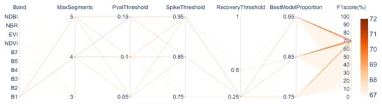
Figure 7.
Combinations of LandTrendr Parameters and F1 score.
Table 6.
Top 10 parameter combinations for high F1 scores in LandTrendr.
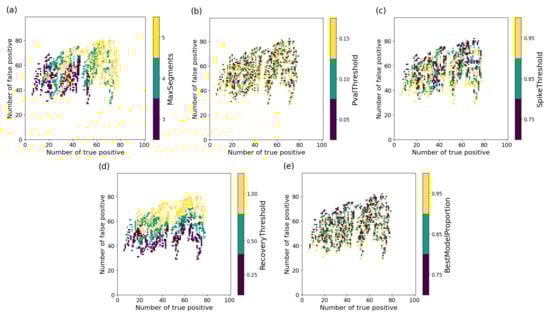
Figure 8.
Relationship between the number of true positives and false positives in LandTrendr for different parameter settings. Each subplot shows the effect of varying (a) MaxSegments, (b) PvalThreshold, (c) SpikeThreshold, (d) RecoveryThreshold, and (e) BestModelProportion. The color indicates the parameter value.
Figure 9 illustrates LandTrendr outputs at an example point that transitioned from Forest to Urban in 2015 as an example. Using B1 as the input, both the optimized parameter settings (Figure 9a) and the default settings (Figure 9b) correctly detected urban land cover change, whereas using NDVI as the input, both the optimized settings (Figure 9c) and the default settings (Figure 9d) failed to detect this change. For (a), the parameters were: , , , , and . For (c), the parameters were: , , , , and . For (b) and (d), the following default parameters were used: , , , , and .
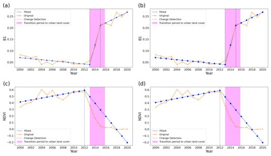
Figure 9.
LandTrendr outputs at a point that transitioned from Forest to Urban in 2015. (a) B1 with the optimized parameter configuration, (b) B1 with default parameters, (c) NDVI with the optimized parameter configuration, and (d) NDVI with default parameters. Both (a,b) successfully detect the transition to urban land cover.
3.2.2. CCDC
The association between parameters for the CCDC and F1 scores is shown in Figure 10, and the top ten parameter combinations with the highest F1 scores are listed in Table 7. Figure 11 illustrates how different parameter settings in CCDC affect and . minObservations parameter showed a trade-off: lower values increased but also increased . A setting of 4 produced a high in areas without actual land cover changes, whereas a setting of 6 yielded the highest F1 score. chiSquareProbability parameter performed best at values of 0.8 and 0.9. Although lower chi-square probability values generally increased , this effect was mitigated by setting minObservations to six or eight. For minNumOfYearsScaler, changing the parameter values caused minimal variation in the distributions of and , but settings of 1.00 and 1.33 achieved higher F1 scores. For lambda, setting it to 20 resulted in a higher F1 score. In contrast, setting it to 0 increased but also increased .
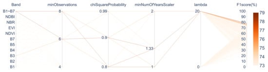
Figure 10.
Combinations of CCDC Parameters and F1 score.
Table 7.
Top 10 parameter combinations for high F1 scores in CCDC.
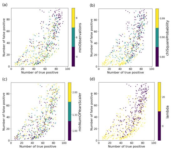
Figure 11.
Relationship between and in the CCDC under different parameter settings. Each subplot shows the effect of varying (a) minObservations, (b) chiSquareProbability, (c) minNumOfYearsScaler, and (d) lambda. The color indicates the parameter value.
Figure 12 illustrates CCDC outputs at a point that transitioned from Farmland to Urban in 2014. Using B1–B7 with the optimized parameter settings (Figure 12a) correctly detected urban land cover change, whereas other settings using B1–B7 with the default settings (Figure 12b), and using NDVI with optimized (Figure 12c) and default settings (Figure 12d) failed to the urban land cover change detection. For (a), the parameters were: , , , and . For (c), the parameters were: , , , and . For both (b) and (d), the following parameters were: , , , and .
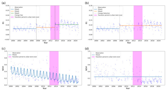
Figure 12.
CCDC outputs at an example point that transitioned from Farmland to Urban in 2014. (a) B1–B7 with the optimized parameters, (b) B1–B7 with default parameters, (c) NDVI with the optimized parameters, and (d) NDVI with default parameters. (a) successfully detects the transition to urban land cover.
3.2.3. BFAST
The association between parameters and F1 scores for BFAST is shown in Figure 13, and the top ten parameter combinations with the highest F1 scores are shown in Table 8. Figure 14 illustrates the effects of the different parameter settings in BFAST affect and . A higher h tends to achieve a higher F1 score, with decreasing while minimally affecting . Setting the Season parameter to none tends to yield a higher F1 score. Although the dummy and harmonic settings increased both and compared to none, this resulted in a lower F1 score. For Breaks, values of 2 and 3 tend to achieve higher F1 scores. Unlike LandTrendr and CCDC, increasing the Break parameter did not significantly increase . The Level parameter for the test threshold had a minimal impact on the F1 scores. Time-series data at 3-month intervals tends to produce a higher F1 score, whereas 16-day interval data showed a high , resulting in a lower F1 score.
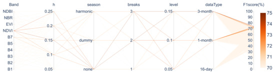
Figure 13.
Combinations of BFAST Parameters and F1 score.
Table 8.
Top 10 parameter combinations for high F1 scores in BFAST.
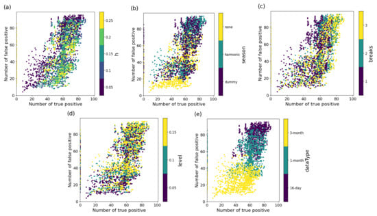
Figure 14.
Relationship between the number of true positives and false positives in BFAST under different parameter settings. Each subplot shows the effect of varying (a) h, (b) season, (c) breaks, (d) level, and (e) dataType. The color indicates the parameter value.
Figure 15 illustrates BFAST outputs at an example point that transitioned from Grassland to Urban in 2014. Using B1 as input with optimized settings (Figure 15a) and with default settings (Figure 15b), both failed to detect urban land cover change, whereas using NDVI as input with both optimized settings (Figure 15c) and the default settings (Figure 15d) successfully detected the change. For (a), the parameters were: h = 0.15, Season = dummy, Breaks = 2, Level = 0.15, and the data type was 3-month. For (c), the parameters were: h = 0.15, Season = none, Breaks = 2, Level = 0.15, and the data type was 3-month. For both (b) and (d), the parameters were used: h = 0.15, Season = harmonic, Breaks = Null, Level = 0.05, and the data type was 3-month.
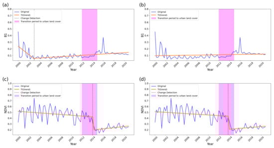
Figure 15.
BFAST outputs at an example point that transitioned from Grassland to Urban in 2014. (a) B1 with the optimized parameter, (b) B1 with default parameters, (c) NDVI with the optimized parameters, and (d) NDVI with default parameters. Both (c,d) successfully detect the transition to urban land cover.
3.3. Analysis of Detection Performance Metrics
In this study, we evaluated 2430 parameter combinations for LandTrendr, 594 for the CCDC, and 4050 for BFAST. Figure 16a–c illustrates the relationship between and for the parameters of each model. LandTrendr (Figure 16a) showed a correlation coefficient of 0.32 between and , indicating a weak linear relationship. In contrast, CCDC (Figure 16b) and BFAST (Figure 16c) showed stronger relationships, with correlation coefficients of 0.72 and 0.52, respectively. This suggests that, for both CCDC and BFAST, increases in are typically accompanied by increases in .
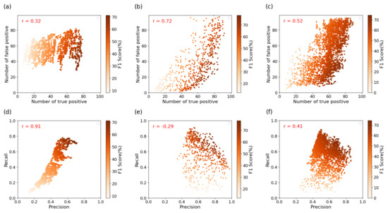
Figure 16.
Relationship between the number of true positive and false positive by (a) LandTrendr, (b) CCDC, and (c) BFAST model, and between Recall and Precision by (d) LandTrendr, (e) CCDC, and (f) BFAST model.
Figure 16d–f show the effect of parameter settings on the relationship between Recall and Precision for each model. LandTrendr (Figure 16d) exhibited a correlation coefficient of 0.91, indicating that a higher recall corresponded to substantially higher precision. The CCDC (Figure 16e) showed the opposite trend, with a correlation coefficient of −0.29, revealing a trade-off in which increased recall led to decreased precision. For BFAST (Figure 16f), despite a positive correlation coefficient of 0.41, precision improvements were modest compared with recall increases.
None of the models achieved both a high recall (>0.8) and precision (>0.8) in our experiments. This indicates an inherent trade-off between increasing and in detection performance. These findings suggest that achieving superior detection performance only by a time-series urban land cover change detection model is challenging, highlighting the need for integrating supplementary techniques, such as machine learning.
3.4. Evaluation of Detection Year
Figure 17 shows the distribution of the predicted land cover change years based on the parameter combinations that achieved the highest F1 scores for each model. On the horizontal axis, 0 represents detection in the year of building completion, while −1 indicates detection one year before completion. The CCDC, with its largest input dataset, typically detects changes during the completion year. LandTrendr and BFAST, using fewer inputs, tended to detect changes one year before completion. Because we defined land change as occurring within two years before completion to account for site preparation and construction time, all models showed frequent detections within this range. This suggests that the models detect land cover changes associated with urbanized land cover developments, including site preparation, rather than solely identifying the building completion year.
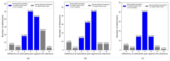
Figure 17.
Histograms of difference from estimated year by (a) LandTrendr, (b) CCDC, and (c) BFAST models with the best combination of parameters against the referenced year. Blue bars indicate the transition period to urban land cover, whereas grey bars represent the period outside of this transition. The definition of this period is provided in Section 2.4.
3.5. F1 Scores for Farmland and Grassland Conversion
Given the high number of target points where Farmland and Grassland were converted to Urban, we evaluated the F1 score separately for each land cover class (Table 9). For clarity, the F1 score for Farmland includes only points that either remained Farmland or were transformed from Farmland to urban areas. Across all bands and indices, the models consistently achieved higher F1 scores for Grassland than for Farmland.
Table 9.
Maximum F1 scores (%) by land cover type (Farmland, Grassland to Urban).
4. Discussion
Using a comprehensive dataset of globally distributed sampling points, we conducted an in-depth analysis examining how parameter settings and input variable selection influenced urban land cover change detection across three time-series algorithms: LandTrendr, CCDC, and BFAST. Our investigation utilized Landsat time-series data to systematically evaluate how these different configurations affected the performance of the algorithms in identifying urban development patterns.
4.1. Model and Parameter Selection
We evaluated F1 scores across numerous parameter combinations: 2430 for LandTrendr, 594 for CCDC, and 4050 for BFAST. Our analysis revealed that both model parameters and input band selection substantially affected accuracy. While previous studies typically relied on arbitrary or default parameter settings for change-detection models [33,34,40,41,42,43,44,45,46,47,49,52,53,58,59], our findings demonstrate that the selection of parameters and input bands directly influences detection accuracy.
4.1.1. Frequency of Input Data
We systematically varied temporal resolution across models: LandTrendr employed 21 annual composites, BFAST utilized three temporal aggregations (16-day, monthly, and quarterly intervals), and CCDC incorporated all available Landsat observations. Our hypothesis that higher temporal frequency would yield superior detection performance was partially supported, as CCDC and BFAST (using more frequent observations) outperformed LandTrendr (using annual composites) in overall F1 scores.
For BFAST, however, the 3-month time-series data achieved the highest F1 score. Using 16-day or 1-month intervals increased in areas where no land cover changes occurred. This suggests that BFAST may interpret minor data fluctuations within the same land cover class when using higher-frequency time-series data. While previous research has often assumed that denser time-series data (such as 16-day intervals) would better capture land cover conditions [37,39,73], our study showed that increasing data frequency does not necessarily improve F1 scores when implementing BFAST. It is crucial to determine the optimal temporal resolution based on the balance between and .
4.1.2. Seasonality
Vegetated land cover typically exhibits a seasonal pattern. While BFAST and CCDC can account for seasonality in time-series data, allowing them to differentiate between seasonal changes and actual land cover changes, LandTrendr only detects sudden and gradual trends, without considering seasonality. In our study, CCDC and BFAST, both capable of capturing seasonality, achieved higher F1 scores than LandTrendr did. This finding suggests that accounting for seasonality may improve performance. However, BFAST achieved the highest F1 score when seasonality was excluded from the parameter settings. When the BFAST parameters were set to account for seasonality, both and increased, resulting in a lower F1 score. Although previous studies have frequently used BFAST’s seasonality parameter [32,53,73,74,75,76], our findings show that including seasonality in parameter settings does not improve the detection accuracy in terms of urban land-cover change detection.
4.2. Advantages of CCDC: Multiband and High-Frequency Data Use
A key advantage of the CCDC algorithm is its ability to process all available Landsat observations using both multiband spectral information and high-frequency temporal data. Unlike LandTrendr, which uses annual composites, CCDC directly processes the complete Landsat time series. This enables the detection of both short-term fluctuations and long-term trends without temporal aggregation. Furthermore, the CCDC processes multiple spectral bands simultaneously. The highest F1 score (78.14%) was achieved when all reflectance bands (B1–B7) were used. This demonstrates how the CCDC effectively combines information across different wavelengths, surpassing models that rely on single bands or indices.
4.3. Challenges for Improving Detection Accuracy
While we evaluated various parameter combinations for each model, all three models resulted in F1 scores below 80%. When we adjusted the parameters to increase , we typically saw a corresponding increase in , whereas attempts to reduce led to a decrease in . These results suggest that parameter adjustments alone within the change-detection model cannot achieve both high and low simultaneously. To improve performance, we may need to integrate the change-detection model with complementary approaches. For instance, we can configure the model to maximize to capture more possible detections, then use machine learning methods such as Support Vector Machines or Random Forests to refine the results by reducing . Future studies will explore the integration of these time-series algorithms with advanced machine learning approaches to overcome the inherent limitations of the accuracy.
4.4. Implications for Urban Expansion Monitoring
This study provides important insights directly relevant to improving urban land cover change detection methods using remote sensing time-series data. Our systematic evaluation across diverse global urban environments demonstrates that any urban land cover change detection model requires careful parameter tuning and spectral selection as inputs. We found the superior performance of CCDC, highlighting the value of leveraging both multiband spectral information and high-frequency temporal data in urban monitoring. These findings bridge the gap between algorithmic evaluation and real-world urban monitoring needs, providing guidance for researchers and practitioners to fully utilize time-series methods for more effective detection of urban expansion.
5. Conclusions
This study provides the first comprehensive evaluation of how parameter configurations influence urban change detection performance across three leading time-series algorithms. Our systematic assessment across diverse global locations yielded the following results: LandTrendr achieved its highest F1 score of 71.29% using B1 as the input band and the parameter settings: , , , , and , while CCDC recorded its peak F1 score of 78.14% when utilizing the full spectral range (B1–B7) with , , , and . BFAST reached its maximum F1 score of 74.32% using NDVI input with , , , by three-month averaged time-series data. CCDC outperformed the other two approaches, achieving its highest accuracy with the full spectral range (B1–B7). Contrary to conventional approaches that prioritize vegetation indices, we found that visible bands (particularly B1 and B2) yield superior urban land cover change detection results. These findings provide critical guidance for satellite-based urban expansion monitoring and highlight the importance of parameter optimization to enhance the application of existing algorithms for urbanization detection.
Despite careful parameter tuning, all three models showed a clear trade-off between true positives and false positives. These metrics were positively correlated, indicating that detection accuracy has inherent limitations when using these models alone. While our findings advance the methodological foundation for remote sensing–based urban monitoring, even optimized algorithms may lack sufficient accuracy for comprehensive urban expansion monitoring. Parameter selection is crucial, yet researchers and practitioners typically use default parameters when applying LandTrendr, CCDC, and BFAST. Our research showed that optimal parameters vary depending on pre-urbanized land cover types. Therefore, it is essential to calibrate parameters and input bands using representative sample points before applying these models to regional-scale studies. Future research should prioritize developing a more accurate, comprehensive, and systematic framework for urban monitoring.
Author Contributions
Conceptualization, T.M. and N.T.; Methodology, T.M. and N.T.; Formal analysis, T.M.; writing—original draft preparation, T.M.; writing—review and editing, N.T.; Supervision, N.T. All authors have read and agreed to the published version of the manuscript.
Funding
This research received no external funding.
Institutional Review Board Statement
Not applicable.
Informed Consent Statement
Not applicable.
Data Availability Statement
The data presented in this study are available on request from the corresponding author.
Acknowledgments
We gratefully acknowledge USGS/NASA for providing Landsat time-series data through Google Earth Engine and thank the developers of the LandTrendr, BFAST, and CCDC algorithms. We appreciate the three anonymous reviewers who provided insightful comments to this manuscript.
Conflicts of Interest
The authors declare no conflicts of interest.
Abbreviations
The following abbreviations are used in this manuscript:
| LandTrendr | Landsat-based detection of Trends in Disturbance and Recovery |
| CCDC | Continuous Change Detection and Classification |
| BFAST | Breaks for Additive Seasonal and Trend |
| NDVI | Normalized Difference Vegetation Index |
| EVI | Enhanced Vegetation Index |
| NBR | Normalized Burn Ratio |
| NDBI | Normalized Difference Built-up Index |
| LULC | Land Use and Land Cover |
| GEE | Google Earth Engine |
Appendix A. Box Plots of F1 Scores for Each Model
Figure A1–Figure A3 display box plots of F1 scores for each input band across the models, illustrating the variation in F1 scores owing to the parameter settings. In LandTrendr, significant fluctuations in F1 scores were observed when EVI and NBR were used as inputs. For the CCDC, noticeable variations in F1 scores were found using B4, NDVI, EVI, and NBR as inputs. In BFAST, large fluctuations in F1 scores were noted when B4, EVI, and NDBI were used as inputs.
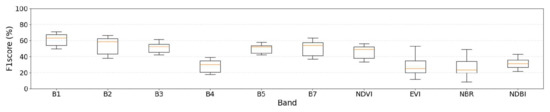
Figure A1.
Box Plot of F1 Scores for LandTrendr according to input band(s).
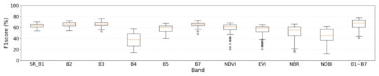
Figure A2.
Box Plot of F1 Scores for CCDC according to input band(s).
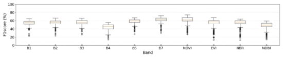
Figure A3.
Box Plot of F1 Scores for BFAST according to input band(s).
References
- United Nations, Department of Economic and Social Affairs. The World’s Cities in 2018—Data Booklet (ST/ESA/SER.A/417). Available online: https://www.un.org/development/desa/pd/sites/www.un.org.development.desa.pd/files/files/documents/2020/Jan/un_2018_worldcities_databooklet.pdf (accessed on 1 May 2025).
- Mahtta, R.; Fragkias, M.; Güneralp, B.; Mahendra, A.; Reba, M.; Wentz, E.A.; Seto, K.C. Urban land expansion: The role of population and economic growth for 300+ cities. npj Urban Sustain. 2022, 2, 5. [Google Scholar] [CrossRef]
- Montgomery, M.R. Urban transformation of the developing world. Science 2008, 319, 761–764. [Google Scholar] [CrossRef] [PubMed]
- Seto, K.C.; Fragkias, M.; Güneralp, B.; Reilly, M.K. A meta-analysis of global urban land expansion. PLoS ONE 2011, 6, e23777. [Google Scholar] [CrossRef] [PubMed]
- Chen, G.; Li, X.; Liu, X.; Chen, Y.; Liang, X.; Leng, J.; Xu, X.; Liao, W.; Qiu, Y.; Wu, Q.; et al. Global projections of future urban land expansion under shared socioeconomic pathways. Nat. Commun. 2020, 11, 537. [Google Scholar] [CrossRef]
- Angel, S.; Parent, J.; Civco, D.L.; Blei, A.; Potere, D. The dimensions of global urban expansion: Estimates and projections for all countries, 2000–2050. Prog. Plann. 2011, 75, 53–107. [Google Scholar] [CrossRef]
- Bren d’Amour, C.; Reitsma, F.; Baiocchi, G.; Barthel, S.; Güneralp, B.; Erb, K.-H.; Haberl, H.; Creutzig, F.; Seto, K.C. Future urban land expansion and implications for global croplands. Proc. Natl. Acad. Sci. USA 2017, 114, 8939–8944. [Google Scholar] [CrossRef]
- Yan, T.; Wang, J.; Huang, J. Urbanization, agricultural water use, and regional and national crop production in China. Ecol. Model. 2015, 318, 226–235. [Google Scholar] [CrossRef]
- van Vliet, J.; Eitelberg, D.A.; Verburg, P.H. A global analysis of land take in cropland areas and production displacement from urbanization. Glob. Environ. Change 2017, 43, 107–115. [Google Scholar] [CrossRef]
- Huang, Q.; Liu, Z.; He, C.; Gou, S.; Bai, Y.; Wang, Y.; Shen, M. The occupation of cropland by global urban expansion from 1992 to 2016 and its implications. Environ. Res. Lett. 2020, 15, 084037. [Google Scholar] [CrossRef]
- Pimonsree, S.; Limsakul, A.; Kammuang, A.; Kachenchart, B.; Kamlangkla, C. Urbanization-induced changes in extreme climate indices in Thailand during 1970–2019. Atmos. Res. 2022, 265, 105882. [Google Scholar] [CrossRef]
- Moazzam, M.F.U.; Doh, Y.H.; Lee, B.G. Impact of urbanization on land surface temperature and surface urban heat island using optical remote sensing data: A case study of Jeju Island, Republic of Korea. Build. Environ. 2022, 222, 109368. [Google Scholar] [CrossRef]
- Yu, W.; Shi, J.; Fang, Y.; Xiang, A.; Li, X.; Hu, C.; Ma, M. Exploration of urbanization characteristics and their effect on the urban thermal environment in Chengdu, China. Build. Environ. 2022, 219, 109150. [Google Scholar] [CrossRef]
- Nguyen, C.T.; Chidthaisong, A.; Limsakul, A.; Varnakovida, P.; Ekkawatpanit, C.; Diem, P.K.; Diep, N.T.H. How do disparate urbanization and climate change imprint on urban thermal variations? A comparison between two dynamic cities in Southeast Asia. Sustain. Cities Soc. 2022, 82, 103882. [Google Scholar] [CrossRef]
- Mohan, M.; Kandya, A. Impact of urbanization and land-use/land-cover change on diurnal temperature range: A case study of tropical urban airshed of India using remote sensing data. Sci. Total Environ. 2015, 506, 453–465. [Google Scholar] [CrossRef]
- Kalnay, E.; Cai, M. Impact of urbanization and land-use change on climate. Nature 2003, 423, 528–531. [Google Scholar] [CrossRef]
- Wu, Y.; Shen, J.; Zhang, X.; Skitmore, M.; Lu, W. The impact of urbanization on carbon emissions in developing countries: A Chinese study based on the U-Kaya method. J. Clean. Prod. 2016, 135, 589–603. [Google Scholar] [CrossRef]
- Wulder, M.A.; White, J.C.; Loveland, T.R.; Woodcock, C.E.; Belward, A.S.; Cohen, W.B.; Fosnight, E.A.; Shaw, J.; Masek, J.G.; Roy, D.P. The global Landsat archive: Status, consolidation, and direction. Remote Sens. Environ. 2016, 185, 271–283. [Google Scholar] [CrossRef]
- U.S. Geological Survey. Landsat 5. Available online: https://www.usgs.gov/landsat-missions/landsat-5 (accessed on 2 October 2024).
- U.S. Geological Survey. Landsat 7. Available online: https://www.usgs.gov/landsat-missions/landsat-7 (accessed on 2 October 2024).
- Roy, D.P.; Wulder, M.A.; Loveland, T.R.; Woodcock, C.E.; Allen, R.G.; Anderson, M.C.; Helder, D.; Irons, J.R.; Johnson, D.M.; Kennedy, R.; et al. Landsat-8: Science and product vision for terrestrial global change research. Remote Sens. Environ. 2014, 145, 154–172. [Google Scholar] [CrossRef]
- Megahed, Y.; Cabral, P.; Silva, J.; Caetano, M. Land cover mapping analysis and urban growth modelling using remote sensing techniques in Greater Cairo Region—Egypt. ISPRS Int. J. Geo-Inf. 2015, 4, 1750–1769. [Google Scholar] [CrossRef]
- Abd El-kawy, O.R.; Ismail, H.A.; Yehia, H.M.; Allam, M.A. Temporal detection and prediction of agricultural land consumption by urbanization using remote sensing. Egypt. J. Remote Sens. Space Sci. 2019, 22, 237–246. [Google Scholar] [CrossRef]
- Patel, A.; Vyas, D.; Chaudhari, N.; Patel, R.; Patel, K.; Mehta, D.J. Novel approach for the LULC change detection using GIS & Google Earth Engine through spatiotemporal analysis to evaluate the urbanization growth of Ahmedabad city. Results Eng. 2024, 21, 101788. [Google Scholar] [CrossRef]
- Rizvi, S.H.; Fatima, H.; Iqbal, M.J.; Alam, K. The effect of urbanization on the intensification of SUHIs: Analysis by LULC on Karachi. J. Atmos. Sol.-Terr. Phys. 2020, 207, 105374. [Google Scholar] [CrossRef]
- Liu, L.; Zhang, X.; Zhao, T.; Gao, Y.; Chen, X.; Mi, J. GISD30: Global 30 m impervious surface dynamic dataset from 1985 to 2020 using time-series Landsat imagery on the Google Earth Engine platform. Earth Syst. Sci. Data Discuss. 2022, 4, 1831–1856. [Google Scholar] [CrossRef]
- Lu, H.; Wang, R.; Ye, R.; Fan, J. Monitoring long-term spatiotemporal dynamics of urban expansion using multi-source remote sensing images and historical maps: A case study of Hangzhou, China. Land 2023, 12, 144. [Google Scholar] [CrossRef]
- Tsutsumida, N.; Comber, A.; Barrett, K.; Saizen, I.; Rustiadi, E. Sub-pixel classification of MODIS EVI for annual mappings of impervious surface areas. Remote Sens. 2016, 8, 143. [Google Scholar] [CrossRef]
- Tsutsumida, N.; Comber, A.J. Measures of spatio-temporal accuracy for time series land cover data. Int. J. Appl. Earth Obs. Geoinf. 2015, 41, 46–55. [Google Scholar] [CrossRef]
- Kennedy, R.E.; Yang, Z.; Cohen, W.B. Detecting trends in forest disturbance and recovery using yearly Landsat time series: 1. LandTrendr—Temporal segmentation algorithms. Remote Sens. Environ. 2010, 114, 2897–2910. [Google Scholar] [CrossRef]
- Zhu, Z.; Woodcock, C.E. Continuous change detection and classification of land cover using all available Landsat data. Remote Sens. Environ. 2014, 144, 152–171. [Google Scholar] [CrossRef]
- Verbesselt, J.; Hyndman, R.; Newnham, G.; Culvenor, D. Detecting trend and seasonal changes in satellite image time series. Remote Sens. Environ. 2010, 114, 106–115. [Google Scholar] [CrossRef]
- Yan, X.; Wang, J. Dynamic monitoring of urban built-up object expansion trajectories in Karachi, Pakistan with time series images and the LandTrendr algorithm. Sci. Rep. 2021, 11, 23118. [Google Scholar] [CrossRef]
- Mugiraneza, T.; Nascetti, A.; Ban, Y. Continuous monitoring of urban land cover change trajectories with Landsat time series and LandTrendr-Google Earth Engine cloud computing. Remote Sens. 2020, 12, 2883. [Google Scholar] [CrossRef]
- Chaudhuri, G.; Mainali, K.P.; Mishra, N.B. Analyzing the dynamics of urbanization in Delhi National Capital Region in India using satellite image time-series analysis. Environ. Plan. B Urban Anal. City Sci. 2022, 49, 368–384. [Google Scholar] [CrossRef]
- Pandey, B.; Zhang, Q.; Seto, K.C. Time series analysis of satellite data to characterize multiple land use transitions: A case study of urban growth and agricultural land loss in India. J. Land Use Sci. 2018, 13, 221–237. [Google Scholar] [CrossRef]
- Tsutsumida, N.; Saizen, I.; Matsuoka, M.; Ishii, R. Land cover change detection in Ulaanbaatar using the breaks for additive seasonal and trend method. Land 2013, 2, 534–549. [Google Scholar] [CrossRef]
- Yang, Y.; Erskine, P.D.; Lechner, A.M.; Mulligan, D.; Zhang, S.; Wang, Z. Detecting the dynamics of vegetation disturbance and recovery in surface mining area via Landsat imagery and LandTrendr algorithm. J. Clean. Prod. 2018, 178, 353–362. [Google Scholar] [CrossRef]
- Wu, L.; Li, Z.; Liu, X.; Zhu, L.; Tang, Y.; Zhang, B.; Xu, B.; Liu, M.; Meng, Y.; Liu, B. Multi-type forest change detection using BFAST and monthly Landsat time series for monitoring spatiotemporal dynamics of forests in subtropical wetland. Remote Sens. 2020, 12, 341. [Google Scholar] [CrossRef]
- Bullock, E.L.; Woodcock, C.E.; Olofsson, P. Monitoring tropical forest degradation using spectral unmixing and Landsat time series analysis. Remote Sens. Environ. 2020, 238, 110968. [Google Scholar] [CrossRef]
- Shen, Q.; Gao, G.; Duan, Y.; Chen, L. Long-term continuous changes of vegetation cover in desert oasis of a hyper-arid endorheic basin with LandTrendr algorithm. Ecol. Indic. 2024, 166, 112418. [Google Scholar] [CrossRef]
- Qiu, D.; Liang, Y.; Shang, R.; Chen, J.M. Improving LandTrendr forest disturbance mapping in China using multi-season observations and multispectral indices. Remote Sens. 2023, 15, 2381. [Google Scholar] [CrossRef]
- Li, L.; Du, J.; Wu, J.; Sheng, Z.; Zhu, X.; Song, Z.; Zhai, G.; Chong, F. Evaluating the multidimensional stability of regional ecosystems using the LandTrendr algorithm. Remote Sens. 2024, 16, 3762. [Google Scholar] [CrossRef]
- Ding, N.; Li, M. Mapping forest abrupt disturbance events in southeastern China—Comparisons and tradeoffs of Landsat time series analysis algorithms. Remote Sens. 2023, 15, 5408. [Google Scholar] [CrossRef]
- Souza, A.A.; Galvão, L.S.; Korting, T.S.; Almeida, C.A. On a data-driven approach for detecting disturbance in the Brazilian savannas using time series of vegetation indices. Remote Sens. 2021, 13, 4959. [Google Scholar] [CrossRef]
- Yin, X.; Kou, W.; Yun, T.; Gu, X.; Lai, H.; Chen, Y.; Wu, Z.; Chen, B. Tropical forest disturbance monitoring based on multi-source time series satellite images and the LandTrendr algorithm. Forests 2022, 13, 2038. [Google Scholar] [CrossRef]
- Mardian, J.; Berg, A.; Daneshfar, B. Evaluating the temporal accuracy of grassland to cropland change detection using multi-temporal image analysis. Remote Sens. Environ. 2021, 255, 112292. [Google Scholar] [CrossRef]
- Zhu, L.; Liu, X.; Wu, L.; Tang, Y.; Meng, Y. Long-term monitoring of cropland change near Dongting Lake, China, using the LandTrendr algorithm with Landsat imagery. Remote Sens. 2019, 11, 1234. [Google Scholar] [CrossRef]
- Liu, A.; Chen, Y.; Cheng, X. Monitoring thermokarst lake drainage dynamics in Northeast Siberian coastal tundra. Remote Sens. 2023, 15, 4396. [Google Scholar] [CrossRef]
- Chai, X.R.; Li, M.; Wang, G.W. Characterizing surface water changes across the Tibetan Plateau based on Landsat time series and LandTrendr algorithm. Eur. J. Remote Sens. 2022, 55, 251–262. [Google Scholar] [CrossRef]
- Lothspeich, A.C.; Knight, J.F. The applicability of LandTrendr to surface water dynamics: A case study of Minnesota from 1984 to 2019 using Google Earth Engine. Remote Sens. 2022, 14, 2662. [Google Scholar] [CrossRef]
- Wang, M.; Mao, D.; Wang, Y.; Li, H.; Zhen, J.; Xiang, H.; Ren, Y.; Jia, M.; Song, K.; Wang, Z. Interannual changes of urban wetlands in China’s major cities from 1985 to 2022. ISPRS J. Photogramm. Remote Sens. 2024, 209, 383–397. [Google Scholar] [CrossRef]
- Mendes, M.P.; Rodriguez-Galiano, V.; Aragones, D. Evaluating the BFAST method to detect and characterise changing trends in water time series: A case study on the impact of droughts on the Mediterranean climate. Sci. Total Environ. 2022, 846, 157428. [Google Scholar] [CrossRef]
- Liu, Y.; Xie, M.; Liu, J.; Wang, H.; Chen, B. Vegetation disturbance and recovery dynamics of different surface mining sites via the LandTrendr algorithm: Case study in Inner Mongolia, China. Land 2022, 11, 856. [Google Scholar] [CrossRef]
- Xie, J.; Liu, Y.; Xie, M.; Xia, L.; Yang, R.; Li, J. Exploring the restoration stability of abandoned open-pit mines by vegetation resilience indicator based on the LandTrendr algorithm. Ecol. Indic. 2024, 166, 112392. [Google Scholar] [CrossRef]
- Guo, J.; Li, Q.; Xie, H.; Li, J.; Qiao, L.; Zhang, C.; Yang, G.; Wang, F. Monitoring of vegetation disturbance and restoration at the dumping sites of the Baorixile open-pit mine based on the LandTrendr algorithm. Int. J. Environ. Res. Public Health 2022, 19, 9066. [Google Scholar] [CrossRef] [PubMed]
- Xiao, W.; Deng, X.; He, T.; Chen, W. Mapping annual land disturbance and reclamation in a surface coal mining region using Google Earth Engine and the LandTrendr algorithm: A case study of the Shengli Coalfield in Inner Mongolia, China. Remote Sens. 2020, 12, 1612. [Google Scholar] [CrossRef]
- Zhang, L.; Zhao, Y.; Ren, H.; Xiao, W.; Li, Z. Vegetation resilience evaluation of coal waste dumps after reclamation in arid and semi-arid mining areas based on temporal satellite imagery. Land Degrad. Dev. 2025, 36, 1724–1735. [Google Scholar] [CrossRef]
- Zhang, M.; He, T.; Li, G.; Xiao, W.; Song, H.; Lu, D.; Wu, C. Continuous detection of surface-mining footprint in copper mine using Google Earth Engine. Remote Sens. 2021, 13, 4273. [Google Scholar] [CrossRef]
- Yan, J.; He, H.; Wang, L.; Zhang, H.; Liang, D.; Zhang, J. Inter-comparison of four models for detecting forest fire disturbance from MOD13A2 time series. Remote Sens. 2022, 14, 1446. [Google Scholar] [CrossRef]
- Pasquarella, V.J.; Arévalo, P.; Bratley, K.H.; Bullock, E.L.; Gorelick, N.; Yang, Z.; Kennedy, R.E. Demystifying LandTrendr and CCDC temporal segmentation. Int. J. Appl. Earth Obs. Geoinf. 2022, 110, 102806. [Google Scholar] [CrossRef]
- Zurqani, H.A.; Post, C.J.; Mikhailova, E.A.; Sheppard, D.; Sharp, J.L. Mapping urbanization trends in a forested landscape using Google Earth Engine. Remote Sens. Earth Syst. Sci. 2019, 2, 173–182. [Google Scholar] [CrossRef]
- Lynch, P.; Blesius, L.; Hines, E. Classification of urban area using multispectral indices for urban planning. Remote Sens. 2020, 12, 2503. [Google Scholar] [CrossRef]
- Yasin, M.Y.; Abdullah, J.; Noor, N.M.; Yusoff, M.M.; Noor, N.M. Landsat observation of urban growth and land use change using NDVI and NDBI analysis. IOP Conf. Ser. Earth Environ. Sci. 2022, 1067, 012037. [Google Scholar] [CrossRef]
- Estoque, R.C.; Murayama, Y. Classification and change detection of built-up lands from Landsat-7 ETM+ and Landsat-8 OLI/TIRS imageries: A comparative assessment of various spectral indices. Ecol. Indic. 2015, 56, 205–217. [Google Scholar] [CrossRef]
- Sharma, R.; Joshi, P.K. Mapping environmental impacts of rapid urbanization in the National Capital Region of India using remote sensing inputs. Urban Clim. 2016, 15, 70–82. [Google Scholar] [CrossRef]
- Reba, M.; Seto, K.C. A systematic review and assessment of algorithms to detect, characterize, and monitor urban land change. Remote Sens. Environ. 2020, 242, 111739. [Google Scholar] [CrossRef]
- Murakami, T. Global Urbanization Point Dataset. Zenodo 2025. [Google Scholar] [CrossRef]
- Gorelick, N.; Hancher, M.; Dixon, M.; Ilyushchenko, S.; Thau, D.; Moore, R. Google Earth Engine: Planetary-scale geospatial analysis for everyone. Remote Sens. Environ. 2017, 202, 18–27. [Google Scholar] [CrossRef]
- Carlson, T.N.; Ripley, D.A. On the relation between NDVI, fractional vegetation cover, and leaf area index. Remote Sens. Environ. 1997, 62, 241–252. [Google Scholar] [CrossRef]
- Zha, Y.; Gao, J.; Ni, S. Use of normalized difference built-up index in automatically mapping urban areas from TM imagery. Int. J. Remote Sens. 2003, 24, 583–594. [Google Scholar] [CrossRef]
- Hyndman, R.J.; Khandakar, Y. Automatic time series forecasting: The forecast package for R. J. Stat. Softw. 2008, 27, 1–22. [Google Scholar] [CrossRef]
- Fang, X.; Zhu, Q.; Ren, L.; Chen, H.; Wang, K.; Peng, C. Large-scale detection of vegetation dynamics and their potential drivers using MODIS images and BFAST: A case study in Quebec, Canada. Remote Sens. Environ. 2018, 206, 391–402. [Google Scholar] [CrossRef]
- He, B.; Chang, J.; Wang, Y.; Wang, Y.; Zhou, S.; Chen, C. Spatio-temporal evolution and non-stationary characteristics of meteorological drought in inland arid areas. Ecol. Indic. 2021, 126, 107644. [Google Scholar] [CrossRef]
- Watts, L.M.; Laffan, S.W. Effectiveness of the BFAST algorithm for detecting vegetation response patterns in a semi-arid region. Remote Sens. Environ. 2014, 154, 234–245. [Google Scholar] [CrossRef]
- Lu, M.; Pebesma, E.; Sanchez, A.; Verbesselt, J. Spatio-temporal change detection from multidimensional arrays: Detecting deforestation from MODIS time series. ISPRS J. Photogramm. Remote Sens. 2016, 117, 227–236. [Google Scholar] [CrossRef]
Disclaimer/Publisher’s Note: The statements, opinions and data contained in all publications are solely those of the individual author(s) and contributor(s) and not of MDPI and/or the editor(s). MDPI and/or the editor(s) disclaim responsibility for any injury to people or property resulting from any ideas, methods, instructions or products referred to in the content. |
© 2025 by the authors. Licensee MDPI, Basel, Switzerland. This article is an open access article distributed under the terms and conditions of the Creative Commons Attribution (CC BY) license (https://creativecommons.org/licenses/by/4.0/).