Abstract
Rubber Tree (Hevea brasiliensis) phenology critically influences tropical plantation productivity and carbon cycling, yet topography and climate impacts remain unclear. By integrating multi-sensor remote sensing (2001–2020) and Google Earth Engine, this study analyzed spatiotemporal dynamics in Hainan Island, China. Results reveal that both the start (SOS occurred between early and late March: day of year, DOY 60–81) and end (EOS occurred late January to early February: DOY 392–406, counted from the previous year) of the growing season exhibit progressive delays from the southeast to northwest, yielding a 10–11 month growing season length (LOS). Significantly, LOS extended by 4.9 days per decade (p < 0.01), despite no significant trends in SOS advancement (−1.1 days per decade) or EOS delay (+3.7 days per decade). Topographic modulation was evident: the SOS was delayed by 0.27 days per 100 m elevation rise (p < 0.01), while the EOS was delayed by 0.07 days per 1° slope increase (p < 0.01). Climatically, a 100 mm precipitation increase advanced SOS/EOS by approximately 1.0 day (p < 0.05), preseasonally, a 1 °C February temperature rise advanced the SOS and EOS by 0.49 and 0.53 days, respectively, and a 100 mm January precipitation increase accelerated EOS by 2.7 days (p < 0.01). These findings advance our mechanistic understanding of rubber phenological responses to climate and topographic gradients, providing actionable insights for sustainable plantation management and tropical forest ecosystem adaptation under changing climatic conditions.
1. Introduction
Vegetation phenology—the study of temporal changes in plant life cycles—serves as a sensitive indicator of climate variability [1]. It provides valuable insights into the historical, present, and future statuses of ecosystems [2]. In tropical regions, stable temperature and precipitation patterns promote continuous vegetation growth with minimal dormancy and subtle seasonal variations [3,4]. However, insufficient long-term field observations limit our understanding of tropical vegetation phenology and its responses to global climate change [5,6], which has led to critical knowledge gaps in quantifying topographic mediation of microclimate–phenology interactions and developing species-specific remote sensing methods for tropical tree crops [7]. Moreover, translating phenological shifts into actionable management thresholds remains a challenge [8].
Traditionally, forest phenology has been monitored through ground-based observations [9,10,11]. While these methods yield high accuracy, they are inherently time-consuming and offer limited spatial coverage [12]. In contrast, satellite remote sensing delivers extensive spatial coverage, rapid data acquisition, and consistent repeatability, making it an ideal tool for monitoring phenological changes in forest cover [13]. Key phenological metrics—namely, the start of the growing season (SOS), the end of the growing season (EOS), and the length of the growing season (LOS)—can be extracted from time series of spectral indices, such as the Normalized Difference Vegetation Index (NDVI) derived from optical satellite imagery. Frequently employed datasets include optical images from the Moderate Resolution Imaging Spectroradiometer (MODIS) [14,15], Landsat [16,17], and Sentinel-2 [18,19]. Additionally, due to its strong association with photosynthetic activity, Solar-Induced Chlorophyll Fluorescence (SIF) is increasingly utilized for phenological monitoring [20,21]. Although coarse-resolution satellite data from systems like MODIS and SIF provide broad coverage and frequent revisit rates—beneficial for large-scale phenological studies—challenges persist in tropical regions. Frequent cloud cover often results in gaps within medium-to-high-resolution time series datasets, complicating continuous phenological monitoring [5,22]. Therefore, any long-term phenological investigation in these regions must delicately balance spatial resolution, temporal continuity, and data availability.
Rubber trees (Hevea brasiliensis) are essential for natural rubber production and are widely cultivated in tropical regions, playing a critical economic role [23,24]. As a seasonally deciduous species, the phenological characteristics, particularly leaf flushing and defoliation cycles, directly govern growth efficiency and latex yield by regulating photosynthetic capacity and resource allocation [25,26,27]. Traditional phenological studies have primarily targeted practical applications, such as seedling breeding, rubber tapping schedules, and resilience enhancement [18,28]. With the advancement of remote sensing technology, researchers have increasingly adopted such methods to monitor rubber phenology indicators [29,30]. Tropical environments pose unique challenges for phenological monitoring. Extreme weather events (typhoons, cold spells, droughts) and intercropping practices with phenologically distinct understory vegetation create significant spatial variability [31,32]. Furthermore, frequent cloud cover and highly fragmented plantation landscapes hinder the establishment of a consistent time series using a single satellite sensor [33,34].
Hainan Island, China—the world’s northernmost large-scale rubber-producing region (18–20°N)—exhibits unique climatic characteristics, notably a distinct alternation between dry and rainy seasons [20,35,36]. Previous satellite-derived phenological studies in this region have yielded contradictory trends. One study found that the SOS advanced at 0.94 days per year over 2001–2015 [35], while another showed non-significant delays (0.20 days per year) through 2021 [20]. Such discrepancies likely arise from short-term observational biases, spatial oversimplification (e.g., neglecting elevation gradients and slopes) [27], and insufficient attention to EOS dynamics, which are critical for yield optimization [36,37]. Moreover, reliance on single-sensor approaches, primarily MODIS and SIF, restricts the ability to capture the complex phenological variations within these fragmented rubber plantations accurately [35,37]. Consequently, there is an urgent need to harness multi-sensor remote sensing data and apply quantitative analysis methods to elucidate the impacts of climate and topography on rubber phenology [38,39].
This study aims to investigate the inter-annual phenological variations in rubber plantations in Hainan Island, with a particular focus on their sensitivity to climate and topographical factors. The objectives are threefold: (1) to evaluate the effectiveness and accuracy of remote sensing data in capturing rubber phenological indicators; (2) to quantify the inter-annual trends in rubber phenology over the past two decades; and (3) to elucidate the impacts of climatic and topographical variables on rubber phenology. This research not only deepens our understanding of phenological dynamics in tropical ecosystems but also provides critical insights for sustainable rubber production management and broader climate change adaptation strategies.
2. Materials and Methods
2.1. Study Area
Hainan Island (18°10′N−20°10′N, 108°37′E–111°03′E), located in southern China, experiences an average annual temperature ranging from 23 °C to 27 °C and receives a total annual precipitation of 941 to 2388 mm [20]. The region is characterized by a tropical monsoon climate, which consists of distinct rainy seasons from May to October and dry seasons from November to April [40]. It is noteworthy that the dry season is further marked by drought conditions and lower temperatures [15]. Hainan Island serves as a major rubber plantation base in China, particularly concentrated in the west-central and central regions (e.g., Danzhou City, Qiongzhong County, Baisha County, and Chengmai County). Figure 1 shows the digital elevation model, which provides essential spatial context for the subsequent analyses.
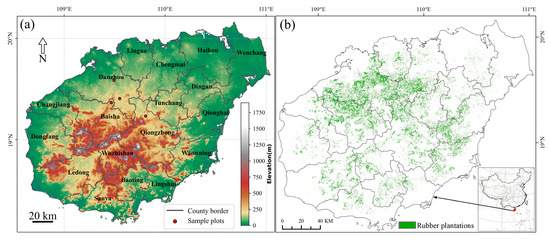
Figure 1.
Overview of the study area: (a) geographical features, including elevation and sample plots; (b) spatial distribution of rubber plantations, with administrative boundaries.
2.2. Data and Processing
2.2.1. Rubber Plantation Map and Field Observations Data
The rubber plantation map was restricted to areas exhibiting spatial stability from 2001 to 2020 (Figure 1). Building on the high-accuracy 2015 map for Hainan Island, which demonstrated producer and user accuracies exceeding 86% at a 30 m spatial resolution, a distribution map for 2020 was subsequently produced [41]. To ensure precise extraction of rubber plantation areas, the 2020 map was integrated with historical rubber plantation imagery from Hainan Island. This masking process allowed for the selection of regions that exhibited negligible changes over the period 2001–2020, thereby facilitating a comprehensive analysis of rubber phenological variations over the past two decades.
In parallel, foliation data from 2001 to 2014 were systematically collected in Danzhou City, Hainan Island (19°24′N, 109°33′E) [37]. In addition, foliation and defoliation observations from 2017 were meticulously gathered from three representative sample areas: Danzhou Liangyuan Experimental Farm (19°35′N, 109°30′E), Baisha County (19°22′N, 109°28′E), and Qiongzhong County (19°14′N, 109°48′E) [35,36]. These field observations were rigorously compared with remote sensing-derived phenological indicators to evaluate the feasibility and accuracy of the remote sensing approach.
2.2.2. Satellite Imagery
Surface reflectance images from Landsat 5, 7, 8, and 9, Sentinel-2, and MODIS from 2001 to 2020 were used to extract phenological indicators of rubber plantations. The specific products used were Landsat collection 2 Level 2 Tier 1, Sentinel-2 Level-2A a combination of daily MOD09GQ and MYD09GQ version 6.1 (250 m resolution). The distributors preprocessed each of these images temporally, spatially, and spectrally using the Google Earth Engine (GEE) cloud platform. In order to obscure shadows and clouds in Landsat series imagery, quality information from the QA_PIXEL band was utilized. In contrast, Sentinel-2 imagery underwent a masking process utilizing a scene-tuned cloud probability layer developed by the Sentinel2-Cloud-Detector library, which employs LightGBM to achieve higher computational efficiency and thin-cloud detection accuracy than traditional methods. In MODIS images, shadows and clouds were obscured by employing the QC_250 m quality control band, with the threshold set at 0.01 ≤ sur_refl_b01 ≤ 0.25 [18]. A simple test revealed that sur_refl_b01 outside this range is often an outlier, resulting in a very low NDVI [42].
2.2.3. Climate Data
Precipitation data were obtained from the Climate Hazards Group InfraRed Precipitation with Station (CHIRPS) dataset, which offers a comprehensive overview of global precipitation patterns at a temporal resolution of one day and a spatial resolution of 0.05 degrees [43]. Temperature information was acquired from the daily Land Surface Temperature (LST) products MOD11A1 and MYD11A1, each providing a spatial resolution of 1 km [44]. Annual and monthly precipitation and temperature values from 2001 to 2020 were accurately calculated and extracted using a geemap-based script [45]. Subsequently, the relationships between monthly temperature, precipitation data, and rubber phenology were systematically analyzed [18,26,46].
2.2.4. DEM Data
The topographic data were obtained from the Advanced Land Observing Satellite (ALOS) World 3D dataset, offering a spatial resolution of 30 m [47]. Slope calculations were conducted using the Google Earth Engine (GEE) platform, followed by data extraction. Analysis of the spatial distribution patterns of rubber plantations in Hainan Island by [48] revealed that 97.75% of plantations occur on slopes < 25° and 91.24% are situated below 300 m altitude. Accordingly, this study focused on areas with slopes < 30° and altitudes < 700 m for in-depth analysis. This selection criterion not only ensured the representativeness of the study area but also accounted for potential marginal distributions of rubber plantations, thereby enhancing the robustness of the spatial analysis.
2.3. Methodology
2.3.1. Method Overview
The methodology of this study is organized into two main sections: the extraction of phenological indicators and the analysis of phenology trends. Each of these processes is elucidated in detail in the subsequent subsections, as illustrated in Figure 2.
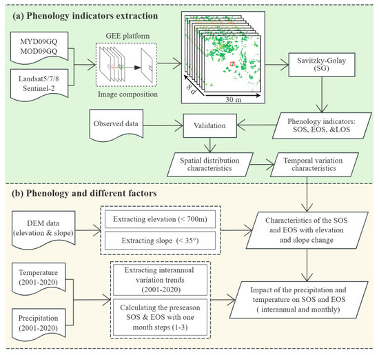
Figure 2.
Flowchart of processes: (a) phenology indicators extraction, and (b) phenology and different factors.
2.3.2. Establishment of NDVI Time Series
We generated a high-resolution (30 m) NDVI time series with 8-day intervals using a hierarchical multi-sensor framework on Google Earth Engine [18]. The NDVI composites were produced in four stages: (1) Prioritizing cloud-free pixels from Landsat/Sentinel-2 (LS2) images acquired within 8-day windows and with ≤20% cloud cover. (2) Filling temporal gaps by using multi-year (±1 year) LS2 NDVI averages whenever current-year data were unavailable. (3) Deriving mean NDVI values from MODIS images by integrating reflectance data from MOD09GQ/MYD09GQ, which were resampled to a 30 m resolution using bilinear interpolation. (4) Addressing persistent gaps by computing multi-year (±1 year) MODIS NDVI averages. Annual composites initiated on January 1st resulted in 46 continuous windows, ensuring full-year coverage while maintaining spatiotemporal consistency at a 30 m resolution.
2.3.3. Defining SOS, EOS, and LOS in Rubber Plantations
Within the TIMESAT 3.3 software, the SOS is defined as the moment when the top buds of rubber plantations shift in color from copper brown to light green, indicating a significant increase in the NDVI. The EOS is identified as the instance when the color changes from bright yellow to nearly full yellow, corresponding to a marked decrease in the NDVI. LOS is subsequently defined as the time interval between the SOS and EOS [18,49]. Ultimately, the Savitzky–Golay (S-G) filter technique was employed, with seasonal amplitude thresholds set at 15% and 20% for the SOS and EOS, respectively [18,50].
2.3.4. Statistical Analysis
The accuracy of phenology extraction was first evaluated using the coefficient of determination (R2). In order to clarify the spatial changes in rubber phenology, we analyzed long-term trends and their climatic drivers. Specifically, the mean values of rubber phenology indicators were calculated over multiple years to assess spatial changes. Trend analysis was performed using two complementary methods: The Theil–Sen slope was employed to robustly estimate the magnitude of the trend (Equation (1)). In parallel, the Mann–Kendall (M-K) test was applied as a non-parametric statistical test to assess the significance of the detected trends in rubber phenology (Equation (2)) [51,52,53]. Additionally, partial correlation coefficients were calculated to precisely evaluate the climate’s response to variations in initial climate conditions and to investigate potential long-term impacts on rubber phenology [29,54] (Equation (3)). The generation of geospatial maps was accomplished utilizing ArcGIS Pro software (version 3.2). Additionally, figures were constructed utilizing Python tools such as Matplotlib (version 3.4.3) and Seaborn (version 0.12.2) [55].
where the trend degree Q represents the direction of the time series, providing essential information about the temporal patterns in rubber phenology. Specifically, xj and xi represent the values of the series at moments j and i, respectively. The interpretation of Q values is straightforward: a positive value (Q > 0) indicates an upward trend, a negative value (Q < 0) suggests a downward trend, and Q = 0 indicates no significant trend.
where is the test statistic that quantifies the monotonic relationship in the data, and is the symbolic function defined for each pair of observations and in the time series (). Together with the Theil–Sen slope, this non-parametric approach provides a comprehensive assessment of both the magnitude and statistical significance of trends in rubber phenology indicators.
The variable rxy[z] represents the relationship between phenological indicators x and climatic parameters y while controlling for the climate metric z, allowing us to isolate specific climate influences. This approach enables a more precise evaluation of climate–phenology relationships by removing confounding effects. The linear correlation coefficients used in this calculation are denoted by rxy, rxz, and rzy, representing the respective pairwise relationships between variables.
3. Results
3.1. Evaluation of the Accuracy and Characterization
Figure 3 demonstrates that the seasonal amplitude method implemented in TIMESAT 3.3 accurately captures the dynamics of both the SOS and EOS in rubber plantations. Satellite imagery obtained from Google Earth Pro for a representative sample area (located at 19°24′N, 109°33′E) captured on 23 March 2014 and 24 February 2015, clearly illustrates the seasonal transitions in foliage color (Figure 3a,b). The high-quality NDVI time series, at 8-day intervals with a spatial resolution of 30 m, clearly depicts the changes in rubber foliage from copper-brown to light-green (indicating an increase in NDVI values for the SOS) and from light-yellow to fully yellow (indicating a decrease in NDVI values for the EOS) (Figure 3(a-1,b-1)). To minimize noise and effectively capture the transitions within the NDVI curves, the S-G filter was applied for smoothing the NDVI time series data (Figure 3c). Validation of the remote sensing estimates was performed by comparing them with field observations. The scatter plots reveal a strong correlation, with data points highly concentrated around the 1:1 line; specifically, the coefficients of determination (R2) for the SOS and EOS were 0.83 and 0.78, respectively (Figure 3d,e). These results underscore the accuracy and reliability of the seasonal amplitude method for phenological extraction, effectively reflecting the leaf expansion and defoliation dynamics of rubber plantations.
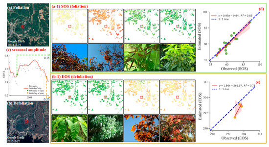
Figure 3.
Extraction and validation of the SOS and EOS using the seasonal amplitude method in TIMESAT 3.3, illustrated with LS2 and MODIS imagery (19°24′N, 109°33′E). (a) Satellite image of a representative area dated 23 March 2014. (a-1) Illustration of foliage change from copper-brown to light-green, indicating an increase in NDVI values at SOS. (b) Satellite image of the same area on 24 February 2015. (b-1) Illustration of foliage change from light-yellow to fully yellow, indicating a decrease in NDVI values at the EOS. (c) Graphical representation of the NDVI curve demonstrating the effects of the seasonal amplitude method, smoothed by the Savitzky–Golay filter. (d,e) Scatter plot and linear regression analysis comparing remote sensing estimates with field observation estimates for the SOS and EOS; the red shades denote the 95% confidence intervals.
3.2. Spatiotemporal Characteristics of Rubber Phenology
Figure 4a–c delineate the pronounced regional specificity of average phenological indicators in rubber plantations over the period 2001–2020. Spatially, a clear pattern of delayed SOS and EOS from southeast to northwest is observed. Specifically, the SOS (day of year, DOY 60–81) occurs predominantly in early to late March, covering 94.39% of the study area, while the EOS (DOY 392–406, counted from the previous year) is mainly observed from late January to early February, spanning 84.95% of the area. The LOS ranges approximately from 10 to 11 months, corresponding to 90.39% of the area.
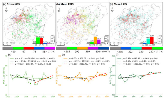
Figure 4.
The spatial and temporal changes in the average phenology indicators in 20 years: the spatial characteristics of the (a) SOS, (b) EOS, and (c) LOS, and the temporal changes in the (d) SOS, (e) EOS, and (f) LOS, respectively. The histogram, situated in the lower right quadrant, provides a graphical representation of the proportional distribution of distinct color bands in relation to the total value.
Figure 4d–f show inter-annual rubber phenology fluctuations. Over the past two decades, the overall trend indicates that the SOS exhibited a non-significant advance at a rate of 1.1 days per decade (r = −0.18, p > 0.05), whereas the EOS showed a non-significant delay at a rate of 3.7 days per decade (r = 0.41, p > 0.05). Notably, the trends of the SOS and EOS displayed similar inter-annual variability. During 2001–2012, the SOS advanced at a non-significant rate of 5.3 days per decade (r = −0.49, p > 0.05), and the EOS advanced at 3.7 days per decade (r = −0.27, p > 0.05). In contrast, the period from 2013 to 2020 saw significant shifts: the SOS extended at a rate of 9.2 days per decade (r = 0.67, p < 0.05) and EOS at 15.9 days per decade (r = 0.75, p < 0.05). Moreover, the LOS exhibited a marked overall increase, advancing by 4.9 days per decade (r = 0.69, p < 0.01).
3.3. Spatial Distribution of Rubber Phenology Variation Trend
Figure 5 depicts the spatial analysis of rubber phenology from 2001 to 2020. Overall, the SOS primarily exhibited an advancing trend with a rate ranging from −0.5 to 0 days per year in 45.75% (Figure 5a). In contrast, the EOS predominantly showed a delaying trend with rates mainly between 0 and 0.5 days per year, covering 40.19% of the areas (Figure 5b). Furthermore, the LOS exhibited an upward trend, with 80.79% of the regions displaying prolonged durations (Figure 5c).
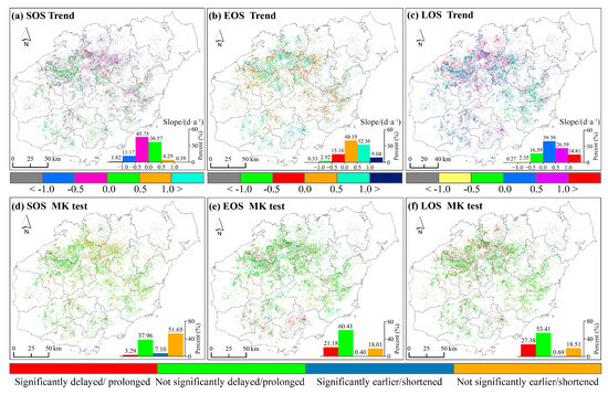
Figure 5.
Spatial distribution of phenology variation trend and proportion of significant pixels (2001–2020). (a–c) Illustrate the spatial distribution of inter-annual variation trends in SOS, EOS, and LOS. (d–f) Depict the significance of the SOS, EOS, and LOS trends as determined by the MK test.
Statistical significance tests revealed that a significant advancement in the SOS (p < 0.05) occurred in 7.10% of the regions, particularly in locations such as Danzhou, Baisha, and Lingao (Figure 5d). Conversely, significant delays in the EOS were observed in 21.18% of the regions, including Danzhou, Baisha, Lingao, Chengmai, Ledong, Sanya, and Baoting (Figure 5e). Regarding LOS, significant extensions were identified in 27.38% of the areas, notably in Danzhou, Baisha, Lingao, and Chengmai (Figure 5f). These results indicate that, while the changes in SOS are not significant in most regions, the delayed trends in the EOS and the prolonged LOS are distinctly prominent across rubber plantations.
3.4. Driving Factors and the Correlation Between Rubber Phenology
3.4.1. Topographic Influences
Figure 6 shows topography’s impact on rubber phenology. The SOS significantly delays by approximately 0.27 days per 100 m elevation increase (p < 0.01). However, the EOS shows no significant relationship with elevation, with only a modest delay of 0.06 days per 100 m (p > 0.05) (Figure 6a). Across different altitudes, the SOS shows a clear gradient with delay rates ranging from 0 to 1.2 days per 100 m, reaching a maximum of 1.1 days (Figure 6b).
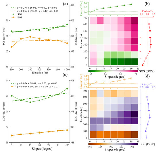
Figure 6.
Topographic influences on rubber phenology: (a) SOS and EOS in relation to elevation. (b) Spatial distribution of SOS relative to mean elevation and slope, analyzed by regression coefficients within each window. Color coding shows mean SOS at per increase 100 m elevation and per increase 1° slope. The upper panel shows its relationship with elevation, and the right panel illustrates the variation in the SOS with slopes. Significance is denoted by solid points (p < 0.05) and non-significance by hollow points (p > 0.05). (c) The SOS and EOS relative to slope. (d) Similar analysis as in (b) but for EOS.
Regarding slope variations, the SOS and EOS exhibit distinct response patterns. As the slope increases, the SOS shows a non-significant delay trend of approximately 0.07 days per degree increment (p > 0.05). In contrast, the EOS demonstrates a significant delay of about 0.06 days per degree (p < 0.01) (Figure 6c). Analysis of maximum delay rates across slope gradients reveals that the SOS and EOS reach maximum delays of approximately 0.16 and 0.17 days per degree, respectively (Figure 6d). Overall, the findings indicate that the SOS is significantly influenced by both elevation and slope, occurring earlier in areas with decreased elevation and increased slope. In contrast, the elevation gradient appears to have little effect on the EOS.
3.4.2. Annual Temperature and Precipitation
The multi-year averages for the SOS and EOS exhibit distinct responses under varying temperature conditions (Figure 7). As temperature increases, the SOS displays a non-significant delay at a rate of approximately 1.38 days per 1 °C (p > 0.05), while the EOS advances significantly at a rate of about 0.62 days per 1 °C (p < 0.01) (Figure 7a,c). However, the correlations between temperature and both the delay in the SOS and the advancement in the EOS were not statistically significant across different temperature gradients (Figure 7b,d).
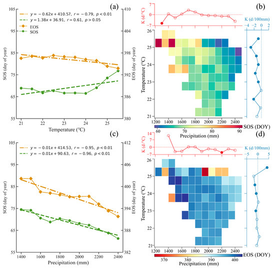
Figure 7.
Climatic influences on rubber phenology: (a) SOS and EOS in relation to temperature. (b) Spatial distribution of SOS relative to mean temperature and precipitation, analyzed by regression coefficients within each window. Color coding shows mean SOS at per increase 1 °C temperature increase and per increase 100 mm precipitation. The upper panel shows its relationship with temperature, and the right panel illustrates the variation in the SOS with precipitation. Significance indicated by solid points (p < 0.05), and non-significance by hollow points (p > 0.05). (c) SOS and EOS in relation to precipitation. (d) Similar to panel (b) but focused on EOS.
Comparatively, the influence of precipitation on phenological changes is more pronounced. With increasing precipitation, both the SOS and EOS demonstrate a significant advancement trend, quantified at roughly 1.00 day per 100 mm (p < 0.05) (Figure 7a,c). Moreover, an analysis across different precipitation gradients revealed that the maximum observed advance reached approximately 3.8 days per 100 mm (Figure 7d).
3.4.3. Sensitivity to Preseason Temperature and Precipitation
Spatial partial correlation analysis revealed the distinct responses of the SOS (January–March) and EOS (December–February) to preseason climatic drivers (Figure 8). Temperature was the primary driver of phenological variations. Significant negative temperature correlations appeared in 78.98% of SOS pixels and 69.42% of EOS pixels. February temperature exerted the strongest influence, significantly affecting 66.45% of SOS pixels and 66.90% of EOS pixels (Figure 8a,c). Each 1 °C increase in February temperature advanced the SOS by 0.49 days (r = −0.66, p < 0.05) and EOS by 0.53 days (r = −0.64, p < 0.05).
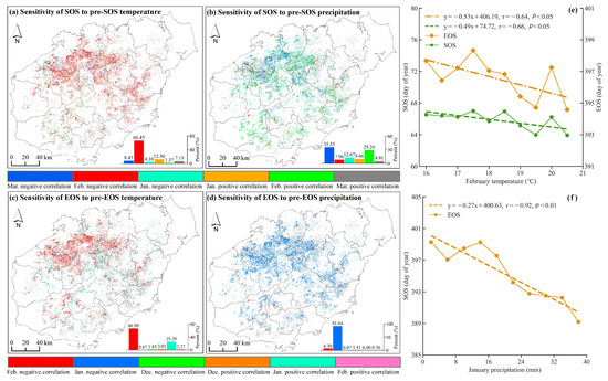
Figure 8.
Spatial correlation of SOS and EOS with key monthly climatic factors: (a,b) Map showing the proportion of areas where the SOS correlates with the most influential month’s temperature and precipitation. (c,d) Similar for EOS; (e) SOS and EOS versus February mean temperature; and (f) SOS versus January total precipitation, respectively. Insets in the bottom right of each panel highlight areas with significant correlations. Different colors in each map indicate varying degrees of correlation.
In contrast, precipitation impacts demonstrated notable spatiotemporal heterogeneity. SOS exhibited variable responses: while February precipitation produced positive correlations in 29.24% of pixels, a shift to negative correlations was observed with March precipitation in 35.55% of pixels. Conversely, the EOS consistently displayed negative correlations with precipitation. This relationship was most pronounced in January, when 91.84% of pixels showed significant responses. Our analysis revealed that a 100 mm increase in January precipitation advanced the EOS by 2.7 days. This strong negative correlation was statistically significant (r = −0.92, p < 0.01) (Figure 8d,f). This differential sensitivity indicates that while SOS precipitation responses vary spatially and temporally, the response mechanism of the EOS to drought is comparatively uniform.
4. Discussion
4.1. Enhanced Monitoring of Rubber Phenology Using Remote Sensing Data
In order to address the challenges posed by incomplete time series, largely due to persistent cloud cover and landscape fragmentation, this study prioritizes the integration of Landsat and Sentinel-2 imagery [19,56]. The complementary features of these sensors not only fill temporal gaps arising from cloud cover but also provide the spatial resolution necessary to monitor small plantations and fragmented landscapes [57]. In addition, the approach of filling missing NDVI data using multi-year (±1 year) MODIS has been well validated, particularly in regions with relatively stable seasonal patterns [58]. As demonstrated by [18], the selection of representative sample points in Yunnan Province confirmed the feasibility of reliably extracting rubber phenology data. This strategy not only enhances data quality but also reduces computational complexity, making large-scale analysis more manageable. The composite algorithm operates with an 8-day temporal resolution and a 30 m spatial resolution. It effectively monitors phenological changes in fragmented rubber plantation landscapes while maintaining essential seasonal characteristics and minimizing data gaps in the time series [59,60,61].
The application of S-G filtering further refines the time series by effectively removing noise and outliers, thereby preserving the integrity of the original signal without the risk of overfitting [33,62]. Compared to alternative filtering techniques, such as double logistic function fitting and the HANTS method, S-G filtering demonstrates superior adaptability and robustness, particularly when applied in complex terrain typical of rubber plantations [63,64]. In the context of phenological indicator extraction, several studies suggest that lower amplitude thresholds (ranging from 10% to 20%) are generally more appropriate for tropical and subtropical regions, owing to the relatively minor seasonal variations in vegetation growth [65]. Consequently, seasonal amplitude thresholds of 15% for the SOS and 20% for the EOS were established [29]. Although these thresholds differ from those used in some previous research, they have proven methodologically robust and yield highly accurate results, as corroborated by ground-based observations [33,35,54]. Thus, the spatial and temporal dynamics of rubber phenology were effectively captured using synthetic remote sensing data, offering invaluable insights for future management of rubber plantations.
4.2. Rubber Phenology Patterns and Influencing Factors
The phenological characteristics of Hainan’s rubber plantations exhibit pronounced spatiotemporal heterogeneity [20,36]. Both the SOS and EOS occur primarily during the dry season (November–April), coinciding with non-significant increases in temperature and precipitation (Figure 9a–c). Spatially, these phenophases display a progressive delay along a southeast-northwest gradient: the SOS initiates between early and late March (DOY 60–81), while the EOS concludes from late January to early February (DOY 392–406) (Figure 4a–c). These findings are largely consistent with both ground-based and remote sensing observations of defoliation and refoliation in rubber plantations [35,66].
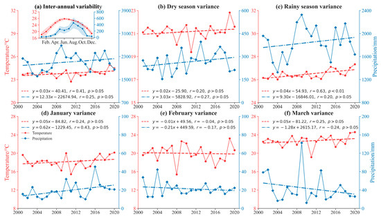
Figure 9.
Annual and monthly mean temperature and precipitation since 2001: (a) Inter-annual variance. (b) Dry season variance. (c) Rainy season variance. (d) January variance. (e) February variance. (f) March variance.
Inter-annual variability in rubber phenology exhibited distinct temporal patterns [20,35]. During 2001–2020, the SOS showed non-significant advancement at 1.1 days per decade, while the EOS exhibited non-significant delay at 3.7 days per decade (Figure 4d–f). Interestingly, during 2013 to 2020, the SOS and EOS displayed significant delays at rates of 9.2 days per decade and 15.9 days per decade, respectively. This phenomenon correlates with Northern Hemisphere climatic variations, highlighting the intensifying impacts of global warming on Hainan’s rubber plantations [54]. Earlier studies documented not statistically significant phenological shifts during 2001–2015, though spring phenology advanced by approximately 0.94 days per year and autumn phenology was delayed by 0.84 days per year [35]. Similarly, the SOS non-significant delaying trend was about 0.20 days per year from 2001 to 2021 [20]. Our island-scale analyses robustly validate these acceleration patterns. The pronounced divergence between the 2001–2012 and 2013–2020 phases primarily originated from intensified extreme climate events. Synergistic effects of climatic forcing and physiological adaptations amplified delayed phenological responses [18,27].
Topographic factors, particularly elevation and slope, significantly influence the temporal and spatial heterogeneity of rubber tree phenology [66]. Specially, for each 100 m increase in elevation, the SOS is delayed by 0.27 days (Figure 6a). This finding is in agreement with the studies, such as those conducted in Xishuangbanna, where the start of refoliation was delayed by about 1.10 days per 50 m increase in elevation [33]. Lower elevations generally experience higher temperatures, which accelerate the cumulative thermal accumulation necessary for growth; in contrast, cooler conditions at elevated terrains contribute to a delayed SOS [4,67].
Similarly, an increase of 1° in slope is associated with an EOS delay of roughly 0.07 days. This effect likely arises from the interplay between modified temperature, humidity, soil moisture retention, and light conditions on steeper gradients [33]. Slope primarily influences rubber tree phenology by modifying soil moisture conditions and light environment [68]. On slopes with poorer soil moisture retention but enhanced light exposure, the compound effect leads to delayed leaf senescence and abscission in rubber trees [22]. It is important to note that the advancement or delay of the SOS and EOS with increasing slope and decreasing elevation may vary across climatic regions and with slope orientation (Figure 6b,d), suggesting a complex, multifactorial interactive process [69,70].
4.3. The Impact of Preseasonal Climatic Conditions on the Rubber Phenology
Rubber phenology is intricately affected by preseasonal climatic conditions, particularly temperature and precipitation patterns [29,66]. Our study found a negative correlation between SOS and both February temperatures (Figure 8a,e). There was a non-significant decreasing trend in inter-annual February temperatures (Figure 9e), while inter-annual March precipitation also showed a non-significant decrease (Figure 9f). A decline in February temperatures enhances rubber plantations’ sensitivity to temperature stimuli, resulting in earlier leaf emergence and accelerated growth. Additionally, rubber plantations are responsive to moisture levels, with both the SOS and EOS significantly advancing with increased precipitation. The SOS and EOS are advanced by 1.00 day for every 100 mm increase in precipitation (Figure 7a,c). Conversely, a decrease in inter-annual March precipitation can lead to inadequate soil moisture, prompting earlier leaf emergence and an advanced SOS [18,54].
The EOS exhibited a negative correlation with January precipitation and February temperature (Figure 8c,d). Trends showed a non-significant increase in inter-annual January precipitation (Figure 9d), while inter-annual February temperatures displayed a non-significant decrease (Figure 9e). An increase in January precipitation provides more adequate soil moisture, while reduced February temperatures have a less stimulating effect [18,32]. Consequently, the EOS is delayed to counteract drought stress effects on phenology [66]. Reference [29] emphasized the significance of the 90-day preseason conditions before to the SOS and EOS in determining the timing of these phenological occurrences. Significantly, excessive precipitation can cause water-logging and root hypoxia, resulting in an earlier EOS [31].
4.4. Study Limitations
While this study offers significant insights into the spatiotemporal variability of rubber phenology, several limitations should be considered. The phenology derived from S-G filtering and the seasonal amplitude method is constrained by the lack of high-quality, long-term observational data on rubber phenology [71]. Enhancing the collection and synchronization of long-term refoliation and defoliation observations is crucial for improving rubber phenology monitoring accuracy [18,66]. This study’s focus on Hainan’s rubber plantations limits the generalizability of its findings to other tropical regions, necessitating broader geographical studies for a more comprehensive understanding [29]. Quantitative gaps persist in stand age effects (e.g., advanced SOS/EOS in PB86 saplings [72]), clone-specific responses (e.g., RRIM 600 vs. GT1 dormancy contrasts [66]), pathogen impacts (e.g., Oidium heveae-induced SOS delays), and soil nutrient mediation via litter cycling [73]. To address these gaps, future research should prioritize (1) multi-sensor fusion to overcome cloud obstruction in tropical monsoons and enhance spatiotemporal consistency [54]; (2) establish standardized dynamic thresholds (SOS/EOS definitions, smoothing windows, iterations) through triadic validation integrating ground-based phenocams, flux towers, and UAV observations; and (3) process explicit modeling incorporating scale-dependent climate drivers, collectively enabling climate-resilient plantation management strategies [18,20]. Despite these limitations, the study offers valuable insights into the spatiotemporal variability of rubber phenology and provides critical data for future research and the development of climate adaptation strategies.
5. Conclusions
This study reveals distinct spatiotemporal patterns in rubber phenology across Hainan Island, with an SOS (DOY 60–81) and EOS (DOY 392–406) exhibiting progressive northwestward delays. The significant extension of the LOS by 4.9 days per decade (p < 0.01) underscores climate-driven phenological shifts, modulated by topographic factors: the SOS delayed by 0.27 days per 100 m elevation rise (p < 0.01), while the EOS delayed by 0.07 days per 1° slope increase (p < 0.01). Climatically, a 100 mm precipitation increase advanced SOS/EOS by approximately 1.0 day (p < 0.05). Climatically, a 100 mm precipitation increase advanced SOS/EOS by approximately 1.0 day (p < 0.05), preseasonally, a 1 °C February temperature rise advanced the SOS and EOS by 0.49 and 0.53 days, respectively; and a 100 mm January precipitation increase accelerated the EOS by 2.7 days (p < 0.01). These quantitative relationships directly inform management protocols: (1) planting early-sprouting clones in high-elevation zones to offset SOS delays; (2) applying organic mulch (e.g., rubber wood chips) when January precipitation is <100 mm to conserve soil moisture, mimicking the EOS advancement effect of 2.7 days per 100 mm rainfall for cold damage mitigation; and (3) advancing tapping schedules by 7–10 days during warm winters to utilize extended LOS. Collectively, understanding these dynamics is crucial for developing strategies to mitigate the impacts of climate change and ensure the long-term productivity of rubber plantations.
Author Contributions
Conceptualization, B.C.; Methodology, H.L. and B.C.; Investigation, G.W., X.Y., and X.W.; Resources, B.C.; Data Curation, W.K., G.L., and T.Y.; Writing—original draft, H.L.; Writing—review and editing, K.J. and Z.W. All authors have read and agreed to the published version of the manuscript.
Funding
This research was funded by the Central Public-interest Scientific Institution Basal Research Fund (1630022023007, 1630022024018), National Key Research and Development Program of China (2024YFD2300901), Natural Science Foundation of Hainan Province (422CXTD527), and Earmarked Fund for China Agriculture Research System (CARS-33).
Data Availability Statement
The annual NDVI time series are available in [18]. Climate data are available in [43,44]. The topographic data are available in [47].
Conflicts of Interest
The authors declare no conflicts of interest.
References
- Richardson, A.D.; Keenan, T.F.; Migliavacca, M.; Ryu, Y.; Sonnentag, O.; Toomey, M. Climate change, phenology, and phenological control of vegetation feedbacks to the climate system. Agric. For. Meteorol. 2013, 169, 156–173. [Google Scholar] [CrossRef]
- Wolkovich, E.M.; Cook, B.I.; Allen, J.M.; Crimmins, T.M.; Betancourt, J.L.; Travers, S.E.; Pau, S.; Regetz, J.; Davies, T.J.; Kraft, N.J.B.; et al. Warming experiments underpredict plant phenological responses to climate change. Nature 2012, 485, 494–497. [Google Scholar] [CrossRef]
- Piao, S.; Liu, Q.; Chen, A.; Janssens, I.A.; Fu, Y.; Dai, J.; Liu, L.; Lian, X.; Shen, M.; Zhu, X. Plant phenology and global climate change: Current progresses and challenges. Glob. Change Biol. 2019, 25, 1922–1940. [Google Scholar] [CrossRef]
- Priyadarshan, P.M. Biology of Hevea Rubber; Springer International Publishing: Cham, Switzerland, 2017. [Google Scholar]
- Abernethy, K.; Bush, E.R.; Forget, P.; Mendoza, I.; Morellato, L.P.C. Current issues in tropical phenology: A synthesis. Biotropica 2018, 50, 477–482. [Google Scholar] [CrossRef]
- Davidson, K.J.; Lamour, J.; Rogers, A.; Ely, K.S.; Li, Q.; McDowell, N.G.; Pivovaroff, A.L.; Wolfe, B.T.; Wright, S.J.; Zambrano, A.; et al. Short-term variation in leaf-level water use efficiency in a tropical forest. New Phytol. 2023, 237, 2069–2087. [Google Scholar] [CrossRef]
- Adams, B.T.; Matthews, S.N.; Iverson, L.R.; Prasad, A.M.; Peters, M.P.; Zhao, K. Spring phenological variability promoted by topography and vegetation assembly processes in a temperate forest landscape. Agric. For. Meteorol. 2021, 308–309, 108578. [Google Scholar] [CrossRef]
- An, S.; Chen, X.; Li, F.; Wang, X.; Shen, M.; Luo, X.; Ren, S.; Zhao, H.; Li, Y.; Xu, L. Long-term species-level observations indicate the critical role of soil moisture in regulating China’s grassland productivity relative to phenological and climatic factors. Sci. Total Environ. 2024, 929, 172553. [Google Scholar] [CrossRef] [PubMed]
- Fu, Y.H.; Zhao, H.; Piao, S.; Peaucelle, M.; Peng, S.; Zhou, G.; Ciais, P.; Huang, M.; Menzel, A.; Peñuelas, J.; et al. Declining global warming effects on the phenology of spring leaf unfolding. Nature 2015, 526, 104–107. [Google Scholar] [CrossRef]
- Nezval, O.; Krejza, J.; Světlík, J.; Šigut, L.; Horáček, P. Comparison of traditional ground-based observations and digital remote sensing of phenological transitions in a floodplain forest. Agric. For. Meteorol. 2020, 291, 108079. [Google Scholar] [CrossRef]
- Berra, E.F.; Gaulton, R. Remote sensing of temperate and boreal forest phenology: A review of progress, challenges and opportunities in the intercomparison of in-situ and satellite phenological metrics. For. Ecol. Manag. 2021, 480, 118663. [Google Scholar] [CrossRef]
- Broich, M.; Huete, A.; Tulbure, M.G.; Ma, X.; Xin, Q.; Paget, M.; Restrepo-Coupe, N.; Davies, K.; Devadas, R.; Held, A. Land surface phenological response to decadal climate variability across Australia using satellite remote sensing. Biogeosciences 2014, 11, 5181–5198. [Google Scholar] [CrossRef]
- Ruan, Y.; Zhang, X.; Xin, Q.; Sun, Y.; Ao, Z.; Jiang, X. A method for quality management of vegetation phenophases derived from satellite remote sensing data. Int. J. Remote Sens. 2021, 42, 5811–5830. [Google Scholar] [CrossRef]
- Ulsig, L.; Nichol, C.J.; Huemmrich, K.F.; Landis, D.R.; Middleton, E.M.; Lyapustin, A.I.; Mammarella, I.; Levula, J.; Porcar-Castell, A. Detecting inter-annual variations in the phenology of evergreen conifers using long-term MODIS vegetation index time series. Remote Sens. 2017, 9, 49. [Google Scholar] [CrossRef]
- Chen, H.; Chen, X.; Chen, Z.; Zhu, N.; Tao, Z. A Primary study on rubber acreage estimation from MODIS-based information in Hainan. Chin. J. Trop. Crops 2010, 31, 1181–1185. (In Chinese) [Google Scholar]
- Dong, J.; Xiao, X.; Chen, B.; Torbick, N.; Jin, C.; Zhang, G.; Biradar, C. Mapping deciduous rubber plantations through integration of PALSAR and multi-temporal Landsat imagery. Remote Sens. Environ. 2013, 134, 392–402. [Google Scholar] [CrossRef]
- Fan, H.; Fu, X.; Zhang, Z.; Wu, Q. Phenology-based vegetation index differencing for mapping of rubber plantations using Landsat OLI data. Remote Sens. 2015, 7, 6041–6058. [Google Scholar] [CrossRef]
- Lai, H.; Chen, B.; Yin, X.; Wang, G.; Wang, X.; Yun, T.; Lan, G.; Wu, Z.; Yang, C.; Kou, W. Dry season temperature and rainy season precipitation significantly affect the spatio-temporal pattern of rubber plantation phenology in Yunnan province. Front. Plant Sci. 2023, 14, 1283315. [Google Scholar] [CrossRef]
- Zhang, X.; Xiao, X.; Qiu, S.; Xu, X.; Wang, X.; Chang, Q.; Wu, J.; Li, B. Quantifying latitudinal variation in land surface phenology of spartina alterniflora saltmarshes across coastal wetlands in China by Landsat 7/8 and Sentinel-2 images. Remote Sens. Environ. 2022, 269, 112810. [Google Scholar] [CrossRef]
- Li, N.; Xiao, J.; Bai, R.; Wang, J.; Wu, L.; Gao, W.; Li, W.; Chen, M.; Li, Q. Preseason sunshine duration determines the start of growing season of natural rubber forests. Int. J. Appl. Earth Obs. 2023, 124, 103513–103522. [Google Scholar] [CrossRef]
- Lu, X.; Liu, Z.; Zhou, Y.; Liu, Y.; An, S.; Tang, J. Comparison of phenology estimated from reflectance-based indices and Solar-Induced Chlorophyll Fluorescence (SIF) observations in a temperate forest using GPP-based phenology as the standard. Remote Sens. 2018, 10, 932. [Google Scholar] [CrossRef]
- Williams, L.J.; Bunyavejchewin, S.; Baker, P.J. Deciduousness in a seasonal tropical forest in western Thailand: Interannual and intraspecific variation in timing, duration and environmental cues. Oecologia 2008, 155, 571–582. [Google Scholar] [CrossRef]
- Qiu, J. Where the rubber meets the garden: China’s leading conservation centre is facing down an onslaught of rubber plantations. Nature 2009, 7227, 246–247. [Google Scholar] [CrossRef] [PubMed]
- Li, Z.; Fox, J.M. Mapping rubber tree growth in mainland Southeast Asia using time-series MODIS 250 m NDVI and statistical data. Appl. Geogr. 2012, 32, 420–432. [Google Scholar] [CrossRef]
- Azizan, F.A.; Astuti, I.S.; Young, A.; Abdul Aziz, A. Rubber leaf fall phenomenon linked to increased temperature. Agric. Ecosyst. Environ. 2023, 352, 108531. [Google Scholar] [CrossRef]
- Yeang, H. Synchronous flowering of the rubber tree (Hevea brasiliensis) induced by high solar radiation intensity. New Phytol. 2007, 175, 283–289. [Google Scholar] [CrossRef]
- Lai, H.; Chen, B.; Yun, T.; Yin, X.; Chen, Y.; Wu, Z.; Kou, W. Research progress on phenology of Hevea brasiliensis under climate change. J. Trop. Subtrop. Bot. 2023, 31, 886–896. [Google Scholar]
- Yin, S.; Chuan, X.; Wang, C.; Zhang, X.; Li, J.; Li, H. Occurrence of powdery mildew on Hevea brasiliensis in Southwest Yunnan. Chin. J. Trop. Agric. 2022, 42, 57–61. (In Chinese) [Google Scholar]
- Azizan, F.A.; Young, A.; Aziz, A.A. Determining the optimum climate preseason for plant phenology analysis using rubber (Hevea brasiliensis) as a model. Remote Sens. Lett. 2022, 13, 1121–1130. [Google Scholar] [CrossRef]
- Zhai, D.; Thaler, P.; Worthy, F.R.; Xu, J. Rubber latex yield is affected by interactions between antecedent temperature, rubber phenology, and powdery mildew disease. Int. J. Biometeorol. 2023, 67, 1569–1579. [Google Scholar] [CrossRef]
- Gutiérrez-Vanegas, A.J.; Correa-Pinilla, D.E.; Gil-Restrepo, J.P.; López-Hernández, F.G.; Guerra-Hincapié, J.J.; Córdoba-Gaona, O.D.J. Foliar and flowering phenology of three rubber (Hevea brasiliensis) clones in the eastern plains of Colombia. Braz. J. Bot. 2020, 43, 813–821. [Google Scholar] [CrossRef]
- Guerra-Hincapié, J.J.; de Jesús Córdoba-Gaona, O.; Gil-Restrepo, J.P.; Monsalve-García, D.A.; Hernández-Arredondo, J.D.; Martínez-Bustamante, E.G. Phenological patterns of defoliation and refoliation processes of rubber tree clones in the Colombian Northwest. Rev. Fac. Nac. Agron. Medellín 2020, 73, 9293–9303. [Google Scholar] [CrossRef]
- Chen, Y.; Khongdee, N.; Wang, Y.; Song, Q.; Lu, D.; Wang, S.; Chen, Y. Spatiotemporal trends of rubber defoliation and refoliation and their responses to abiotic factors in the northern edge of the Asian tropics. Ind. Crops Prod. 2025, 226, 120753. [Google Scholar] [CrossRef]
- Xin, Q.; Broich, M.; Zhu, P.; Gong, P. Modeling grassland spring onset across the western United States using climate variables and MODIS-derived phenology metrics. Remote Sens. Environ. 2015, 161, 63–77. [Google Scholar] [CrossRef]
- Hu, Y.; Dai, S.; Luo, H.; Li, H.; Li, M.; Zheng, Q.; Yu, X.; Li, N. Spatial-temporal variation characteristics of rubber forest phenology in Hainan Island, 2001–2015. Remote Sens. Nat. Resour. 2022, 1, 210–217. (In Chinese) [Google Scholar]
- Li, N.; Bai, R.; Wu, L.; Li, W.; Chen, M.; Chen, X.; Fan, C.-H.; Yang, G.-S. Impacts of future climate change on spring phenology stages of rubber tree in Hainan, China. Chin. J. Appl. Ecol. 2020, 31, 1241–1249. (In Chinese) [Google Scholar]
- Chen, X.; Chen, H.; Li, W.; Liu, S. Remote sensing monitoring of spring phenophase of natural rubber forest in Hainan Province. Chin. J. Agrometeorol. 2016, 37, 111–116. (In Chinese) [Google Scholar]
- Golbon, R.; Cotter, M.; Suerborn, J. Climate change impact assessment on the potential rubber cultivating area in the Greater Mekong Subregion. Environ. Res. Lett. 2018, 13, 84002. [Google Scholar] [CrossRef]
- Wang, Y.; Hollingsworth, P.M.; Zhai, D.; West, C.D.; Green, J.M.H.; Chen, H.; Hurni, K.; Su, Y.; Warren-Thomas, E.; Xu, J.; et al. High-resolution maps show that rubber causes substantial deforestation. Nature 2023, 623, 340–346. [Google Scholar] [CrossRef]
- Xu, G.; Luo, S.; Guo, Q.; Pei, S.; Shi, Z.; Zhu, L.; Zhu, N. Responses of leaf unfolding and flowering to climate change in 12 tropical evergreen broadleaf tree species in Jianfengling, Hainan Island. Chin. J. Plant Ecol. 2014, 38, 585–598. (In Chinese) [Google Scholar]
- Chen, B.; Li, X.; Xiao, X.; Zhao, B.; Dong, J.; Kou, W.; Qin, Y.; Yang, C.; Wu, Z.; Sun, R.; et al. Mapping tropical forests and deciduous rubber plantations in Hainan Island, China by integrating PALSAR 25-m and multi-temporal Landsat images. Int. J. Appl. Earth Obs. 2016, 50, 117–130. [Google Scholar] [CrossRef]
- Tucker, C.J. Red and photographic infrared linear combinations for monitoring vegetation. Remote Sens. Environ. 1979, 2, 127–150. [Google Scholar] [CrossRef]
- Shen, Z.; Yong, B.; Gourley, J.J.; Qi, W.; Lu, D.; Liu, J.; Ren, L.; Hong, Y.; Zhang, J. Recent global performance of the Climate Hazards group Infrared Precipitation (CHIRP) with Stations (CHIRPS). J. Hydrol. 2020, 591, 125284. [Google Scholar] [CrossRef]
- Metz, M.; Andreo, V.; Neteler, M. A new fully gap-free time series of Land Surface Temperature from MODIS LST Data. Remote Sens. 2017, 9, 1333. [Google Scholar] [CrossRef]
- Peterson, P.; Funk, C.C.; Husak, G.J.; Pedreros, D.H.; Landsfeld, M.; Verdin, J.P.; Shukla, S. The Climate Hazards group InfraRed Precipitation (CHIRP) with Stations (CHIRPS): Development and Validation. In Proceedings of the AGU 2013 Fall Meeting, San Francisco, CA, USA, 9–13 December 2013. [Google Scholar]
- Zhai, D.; Yu, H.; Chen, S.; Ranjitkar, S.; Xu, J. Responses of rubber leaf phenology to climatic variations in Southwest China. Int. J. Biometeorol. 2019, 63, 607–616. [Google Scholar] [CrossRef] [PubMed]
- Caglar, B.; Becek, K.; Mekik, C.; Ozendi, M. On the vertical accuracy of the ALOS world 3D-30m digital elevation model. Remote Sens. Lett. 2018, 9, 607–615. [Google Scholar] [CrossRef]
- Li, G.; Kou, W.; Chen, B.; Wu, Z.; Zhang, X.; Yun, T.; Ma, J.; Sun, R.; Li, Y. Spatio-temporal changes of rubber plantations in Hainan Island over the past 30 years. J. Nanjing For. Univ. 2023, 47, 189. (In Chinese) [Google Scholar]
- Jönsson, P.; Eklundh, L. Seasonality extraction by function fitting to time-series of satellite sensor data. IEEE Trans. Geosci. Remote 2002, 40, 1824–1832. [Google Scholar] [CrossRef]
- Wu, C.; Peng, D.; Soudani, K.; Siebicke, L.; Gough, C.M.; Arain, M.A.; Bohrer, G.; Lafleur, P.M.; Peichl, M.; Gonsamo, A.; et al. Land surface phenology derived from normalized difference vegetation index (NDVI) at global FLUXNET sites. Agric. For. Meteorol. 2017, 233, 171–182. [Google Scholar] [CrossRef]
- Kendall, M.G. Rank Correlation Methods; Charles Griffin & Co. Ltd.: London, UK, 1975. [Google Scholar]
- Sen, P.K. Estimates of the regression coefficient based on Kendall’s tau. J. Am. Stat. Assoc. 1968, 63, 1379–1389. [Google Scholar] [CrossRef]
- Theil, H. A rank invariant method of linear and polynomial regression analysis. Indag. Math. 1950, 53, 386–392. [Google Scholar]
- Azizan, F.; Astuti, I.; Aditya, M.; Febbiyanti, T.; Williams, A.; Young, A.; Aziz, A.A. Using multi-temporal satellite data to analyse phenological responses of rubber (Hevea brasiliensis) to climatic variations in South Sumatra, Indonesia. Remote Sens. 2021, 13, 2932. [Google Scholar] [CrossRef]
- Waskom, M.L. Seaborn: Statistical data visualization. J. Open Source Softw. 2021, 6, 3021. [Google Scholar] [CrossRef]
- Olaniyi, O.N.; Szulczyk, K.R. Estimating the economic impact of the white root rot disease on the Malaysian rubber plantations. For. Policy Econ. 2022, 138, 102707. [Google Scholar] [CrossRef]
- Chaves, M.E.D.; Picoli, M.C.A.; Sanches, I.D. Recent applications of Landsat 8/OLI and Sentinel-2/MSI for land use and land cover mapping: A systematic review. Remote Sens. 2020, 12, 3062. [Google Scholar] [CrossRef]
- Chen, G.; Liu, Z.; Wen, Q.; Tan, R.; Wang, Y.; Zhao, J.; Feng, J. Identification of rubber plantations in Southwestern China based on multi-source remote sensing data and phenology windows. Remote Sens. 2023, 15, 1228. [Google Scholar] [CrossRef]
- Laskin, D.N.; McDermid, G.J.; Nielsen, S.E.; Marshall, S.J.; Roberts, D.R.; Montaghi, A. Advances in phenology are conserved across scale in present and future climates. Nat. Clim. Change 2019, 9, 419–425. [Google Scholar] [CrossRef]
- An, L.; Wu, J.; Zhang, Z.; Zhang, R. Failure analysis of a lattice transmission tower collapse due to the super typhoon Rammasun in July 2014 in Hainan Province, China. J. Wind. Eng. Ind. Aerod. 2018, 182, 295–307. [Google Scholar] [CrossRef]
- Augspurger, C.K.; Cheeseman, J.M.; Salk, C.F. Light gains and physiological capacity of understorey woody plants during phenological avoidance of canopy shade. Funct. Ecol. 2005, 19, 537–546. [Google Scholar] [CrossRef]
- Chen, J.; Jönsson, P.; Tamura, M.; Gu, Z.; Matsushita, B.; Eklundh, L. A simple method for reconstructing a high-quality NDVI time-series data set based on the Savitzky–Golay filter. Remote Sens. Environ. 2004, 91, 332–344. [Google Scholar] [CrossRef]
- Atzberger, C.; Eilers, P.H.C. Time series for monitoring vegetation activity and phenology at 10-daily time steps covering large parts of South America. Int. J. Digit. Earth 2011, 4, 365–386. [Google Scholar] [CrossRef]
- Jönsson, P.; Eklundh, L. TIMESAT—A program for analyzing time-series of satellite sensor data. Comput. Geosci. 2004, 30, 833–845. [Google Scholar] [CrossRef]
- Wang, J.; Xiao, X.; Qin, Y.; Dong, J.; Zhang, G.; Kou, W.; Jin, C.; Zhou, Y.; Zhang, Y. Mapping paddy rice planting area in wheat-rice double-cropped areas through integration of Landsat-8 OLI, MODIS, and PALSAR images. Sci. Rep. 2015, 5, 10088. [Google Scholar] [CrossRef] [PubMed]
- Liyanage, K.K.; Khan, S.; Ranjitkar, S.; Yu, H.; Xu, J.; Brooks, S.; Beckschäfer, P.; Hyde, K.D. Evaluation of key meteorological determinants of wintering and flowering patterns of five rubber clones in Xishuangbanna, Yunnan, China. Int. J. Biometeorol. 2019, 63, 617–625. [Google Scholar] [CrossRef]
- Rafferty, N.E.; Diez, J.M.; Bertelsen, C.D. Changing climate drives divergent and nonlinear shifts in flowering phenology across elevations. Curr. Biol. 2020, 30, 432–441. [Google Scholar] [CrossRef] [PubMed]
- Boehm, A.R.; Hardegree, S.P.; Glenn, N.F.; Reeves, P.A.; Moffet, C.A.; Flerchinger, G.N. Slope and Aspect Effects on Seedbed Microclimate and Germination Timing of Fall-Planted Seeds. Rangel. Ecol. Manag. 2021, 75, 58–67. [Google Scholar] [CrossRef]
- Yang, J.; Xu, J.; Zhai, D. Integrating phenological and geographical information with artificial intelligence algorithm to map rubber plantations in Xishuangbanna. Remote Sens. 2021, 13, 2793. [Google Scholar] [CrossRef]
- Razak, J.; Shariff, A.M.; Ahmad, N.B.; Ibrahim Sameen, M. Mapping rubber trees based on phenological analysis of Landsat time series data-sets. Geocarto Int. 2018, 33, 627–650. [Google Scholar] [CrossRef]
- Lin, Y.; Zhang, Y.; Zhou, L.; Li, J.; Zhou, R.; Guan, H.; Zhang, J.; Sha, L.; Song, Q. Phenology-related water-use efficiency and its responses to site heterogeneity in rubber plantations in Southwest China. Eur. J. Agron. 2022, 137, 126519. [Google Scholar] [CrossRef]
- Liyanage, A.D.S. Influence of some factors on the pattern of wintering and on the incidence of oidium leaf fall in clone PB 86. Rubber Res. Inst. Sri Lanka 1976, 53, 31–38. [Google Scholar]
- Li, Y.; Lan, G.; Xia, Y. Rubber trees demonstrate a clear retranslocation under seasonal drought and cold stresses. Front. Plant Sci. 2016, 7, 1907–1918. [Google Scholar] [CrossRef]
Disclaimer/Publisher’s Note: The statements, opinions and data contained in all publications are solely those of the individual author(s) and contributor(s) and not of MDPI and/or the editor(s). MDPI and/or the editor(s) disclaim responsibility for any injury to people or property resulting from any ideas, methods, instructions or products referred to in the content. |
© 2025 by the authors. Licensee MDPI, Basel, Switzerland. This article is an open access article distributed under the terms and conditions of the Creative Commons Attribution (CC BY) license (https://creativecommons.org/licenses/by/4.0/).