Abstract
Biodiversity monitoring requires the discovery of multi-target tracking. The main requirement is not to reduce the localization error but the continuity of the tracks: a high ratio between the duration of the track and the lifetime of the target. To this end, we present an algorithm for detecting and tracking mobile underwater targets that utilizes reflections from active acoustic emission of broadband signals received by a rigid hydrophone array. The method overcomes the problem of a high false alarm rate by applying a tracking approach to the sequence of received reflections. A 2D time–distance matrix is created for the reflections received from each transmitted probe signal by performing delay and sum beamforming and pulse compression. The result is filtered by a 2D constant false alarm rate (CFAR) detector to identify reflection patterns that correspond to potential targets. Closely spaced signals for multiple probe transmissions are combined into blobs to avoid multiple detections of a single target. The position and velocity are estimated using the debiased converted measurement Kalman filter. The results are analyzed for simulated scenarios and for experiments in the Adriatic Sea, where six Global Positioning System (GPS)-tagged gilt-head seabream fish were released and tracked by a dedicated autonomous float system. Compared to four recent benchmark methods, the results show favorable tracking continuity and accuracy that is robust to the choice of detection threshold.
1. Introduction
The detection and tracking of underwater targets is required for applications such as the monitoring of marine fauna [1], identifying schools of fish in commercial ventures [2], and detecting the prey of sperm whales (Physeter macrocephalus) for behavioral analysis [3]. Monitoring is carried out with autonomous floaters or gliders. Real-time analysis allows an immediate response to either report a detection event or approach the source to achieve a better signal-to-noise ratio (SNR). The important requirement in biodiversity assessment is not the localization error but the continuity of the tracks, that is, a high ratio between the duration of the track and the lifetime of the target. We consider two specific applications: (1) the monitoring of deep-sea giant squid (Architeuthis dux) by autonomous gliders to draw conclusions about the behavior of sperm whales, for which squid are a major food source, and (2) the monitoring of fish populations from a floater. The latter is necessary both for regulators, who need to set data-driven policies, and for sustainable fisheries to reduce bycatch by making fishermen aware of the location of fish schools. The first application is considered in the context of a project called CETI (Cetacean Translation Initiative), in which we have set ourselves the ambitious goal of understanding the language of sperm whales by tracking their activity and vocalizations. The second application is in a project called SOUND, where we deploy a swarm of autonomous floaters to monitor the water column in search of schools of fish. In both cases, the monitoring is performed by active acoustics, specifically, by emitting acoustic signals and analyzing their reflections to find moving targets. Images of our glider and floater platforms can be found in Figure 1a,b, respectively. In this paper, we describe our solution for target detection and localization.
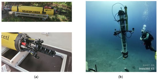
Figure 1.
Platforms used for the task of tracking mobile underwater targets. (a) The CETI glider (built by Alseamar) with an array of hydrophones embedded in the nose section to detect deep-sea squid. Active acoustics performed by an acoustic pinger attached to the glider. Analysis is conducted on board by a Jetson board, and the online change of mission is made possible by a backseat driver. (b) The SOUND floater with an array of hydrophones on the side and a projector on the top. The analysis is performed on a Raspberry Pi board inside the floater, and the detection is shared throughout a swarm of floaters for improved SNR and response.
Underwater, acoustics are the only way to transmit omnidirectional signals over distances in shallow water. RF signals are heavily attenuated underwater and optics suffer from high noise levels during the day. Acoustics can also be used to identify species based on the frequency response of reflections and the speed and movement pattern of the detected target. The detection of underwater targets by active sonar is dominated by the signal-to-clutter ratio (SCR). The level of SCR is measured at the output of the matched filter before processing. The signal is measured at the range and angle of the target as known from the Global Positioning System (GPS), and the noise is measured as the average of all other samples. The SCR therefore includes all reflections that are not associated with the target. Due to the low target strength of fish (in the order of −40 dB [4]), the SCR is likely to be in the order of 0 dB. Therefore, in active acoustic detection, an array of hydrophone receivers is used to utilize the spatial domain by, for example, beamforming [5]. In our case, we use an array of four hydrophones positioned in the plane. The challenge here is to deal with the ambiguity in the angle estimation, which reaches 15° for a plenary array [6]. Another challenge lies in the fast mobility of the tracked target and the possible existence of multiple targets.
1.1. Main Approach
Our multi-target detection and localization solution is based on the tracking approach to analyze the reflections of a transmitted sequence of broadband chirp signals received by an acoustic array. The solution is obtained for a batch of such emissions, and the detection and tracking decision is made at the end of the batch. For the reflections received after each emission, a 2D angle–distance matrix is formed by pulse compression and delay-and-sum beamforming. The samples of this matrix are thresholded by a constant false alarm (CFAR) detector to eliminate weak reflections that may not be associated with the search targets. The remaining samples are grouped into blobs, followed by further filtering to remove detected regions that are too small or too large. To track the targets, we use the debiased converted measurement Kalman filter [7] with a near constant velocity (NCV) dynamical model. The result is a scheme for 2D target tracking whose main advantage is the ease of handling targets with low SCR in a high false alarm rate environment. Instead of following a specific track, e.g., using a Kalman filter, our tracking approach considers all possibilities in a batch. This allows us to avoid the problem of occlusion and mitigate the impact of errors caused by multipath effects, for example.
1.2. Importance and Contribution
When analyzing biodiversity, our goal is to determine the existence of marine biofauna and estimate its biomass. The actual location in relation to the receiver is less important, as the target (e.g., a fish) is highly mobile and a fast response to a detection event is not available. In this context, our goal is to find a robust solution that can handle the case of multiple targets (e.g., a school of fish) in a high-clutter environment and avoid false detections. To this end, our approach relies on the continuity of the track to verify true targets and separate targets, even in the practical case of high spatial ambiguities.
Different from radar applications, due to the limitations of the deploying platform (the floater and glider in our case), underwater spatial signal processing encounters the challenge of small arrays with low aperture. Specifically, in our trials, we consider a system with only four hydrophones with a spacing of <20 cm. Since the available frequency band is small (30–40 kHz in our case) due to channel and hardware limitations, ambiguities in the beam pattern occur, leading to tracking instabilities. This means that targets can disappear and reappear. We address this challenge by offering a tracking approach. Our approach works with a 3D image of possible “blobs” of targets over time. In the tracking approach, detection is not based on a single reflection but on a stack of measurement reflections. For each reflection, “blobs” of possible targets are identified so that the raw acoustic measurements do not need to be stored. While the related tracking approaches follow a single track, this approach enables multi-tracking while detection is performed in a batch of measurements.
Our contributions are twofold:
- 1.
- It is a 2D multi-target scheme for moving-fish identification using omnidirectional active acoustics tailored to a dynamic marine environment. To cope with mismatches in the clutter model, we implemented an adaptive thresholding system that recognizes temporal “blobs” of potential targets as changes from the surrounding.
- 2.
- We merge adaptive beamforming and tracking into a tracking approach that performs simultaneous multi-tracking while reducing the false alarm rate for the special case of non-stable tracks caused by high ambiguities in the beam pattern and intersecting tracks. Incorporating the beamformer into a tracking scheme makes it possible to overcome low signal-to-clutter ratios while utilizing the expected smooth motion of the target. Our method is robust and does not require any prior information in the form of the number of targets or the noise model.
The results of the numerical simulations show the applicability of our method to overcome strong disturbances in scenarios with multiple targets and its advantages over four comparable methods. To demonstrate the applicability of our solution in a real environment, we conducted three experiments in the Adriatic Sea, where six fish were tagged with a Global Positioning System (GPS) receiver, released, and detected by a designated floater, on which we implemented our algorithm. The results show that our algorithm has advantages over the benchmark methods in terms of track continuity and false tracking.
The rest of this article is organized as follows. In Section 2, we give an overview of the state of the art in target detection and the tracking of underwater targets. The system model and key assumptions are presented in Section 3. Our target detection scheme is presented in Section 4, and our multi-target tracking is described in Section 5. Numerical and experimental results are discussed in Section 6. Concluding remarks can be found in Section 7.
2. Literature Review
Starting from the seminal work of Blankman and Popoli [8], there is an extensive literature on radar signal processing. However, there are significant differences between the spatial analysis of radar and sonar signals. The first is the much lower carrier, which together with the small dimensions of the array (due to platform limitations) leads to large ambiguities that affect the stability of the tracks. These instabilities are much worse than with radar. This is partly due to the non-symmetrical environmental-based acoustic propagation and the varying speed of sound at depth. Other differences include the shape and model of the clutter signals, which arise underwater from both reflections at the sea boundary and volume reflections, and the time-varying value of the clutter. Another challenge is the inability to accurately determine the dynamics of targets such as fish, whose motion characteristics range from homogeneous to chaotic. For these reasons, the numerous works dealing with spatial signal processing of underwater sonar data have proposed solutions other than radar-based ones. In the following, we give an overview of these related works.
Target detection using the CFAR method is a common application for underwater monitoring tasks [9]. For clutter mitigation, a cell-averaged CFAR detector is offered in [10], where multiple cells are averaged to determine the detection threshold. Other similar CFAR approaches are the accumulated cell-averaged CFAR [11], in which the accumulated sample matrix is calculated to reduce the computational cost in calculating the detection threshold, and the order statistics CFAR [12], in which noisy samples are attenuated by sorting the samples and selecting only the dominant samples. A detection method that is robust to complex environments is presented in [13]. Here, the 2D matrix is clustered using the K-Means algorithm, and the targets are identified using the resulting binary matrix.
For target tracking, the extended Kalman filter [14] is used due to its simplicity in tracking nonlinear dynamic or measurement models. The method relies on a motion model for the target and a linearization of the measurement model. A version of Kalman tracking for target tracking is the debiased converted measurement Kalman filter [7], in which the nonlinear polar measurements are converted to a linear system of Cartesian coordinates, taking into account the bias due to the nonlinearity of the conversion. A survey of techniques for tracking underwater targets is given in [15], emphasizing the challenge of track continuity of tracking. The use of interacting multiple dynamic models using the Kalman filter is offered in [16], which combines bearing and time-of-arrival estimates. To validate the white noise assumption for Kalman tracking, the work in [17] analyzes the noise distribution in the context of target tracking with a forward-looking sonar. In cases where the SCR is not Gaussian, another option is to use the unscented Kalman filter as proposed in [18], or to learn the noise model in a physics-informed machine learning approach as studied in [19].
For multi-target tracking, the data association of detections into tracks is required. Methods include multi-hypothesis tracking (MHT), in which all possible mappings between detections and tracks are considered, and joint probabilistic data association (JPDA) [20], in which a track is assigned to multiple detections by a probability measure. To reduce the complexity of the MHT filter, a GM-PHD (Gaussian mixture probability hypothesis density) filter is introduced in [21]. This filter has closed-form recursions for the propagation of the state vector and its covariance, and its advantage lies in its practicability for underwater scenarios with multiple targets. In [22], CA-CFAR with threshold segmentation is used to reduce false alarms. The method applies iterative threshold segmentation to reduce false alarms. Another multi-target approach for underwater applications is the sequential Monte Carlo density algorithm [23]. For target detection, the authors offer a combination of CA-CFAR and the K-means detector. To reduce the number of missed tracks, a continuous lost frame threshold is added. More specifically, if the predicted states of a track are not correlated with a target across multiple sonar frames, the state vector and its covariance are replaced by the last updated state of the track. However, the results are limited to high SCR.
Acoustic arrays are used to increase the SCR. In [24], the detection and tracking of underwater targets is performed with a multibeam sonar. Detection is performed by segmenting the sonar image, while the position of the target after detection is determined by its contour position. Target tracking is performed using a particle filter to model the posterior by a series of weighted samples. In [25], the Gaussian mixture cardinalized probability hypothesis density filter is applied to multistatic sonar data. The posterior is estimated by a Gaussian mixture, and the state vector and its covariance are predicted by the EKF. The Gaussian mixture is also used in [26] for a cardinalized likelihood hypothesis filter over real sonar data obtained from a sea trial. This filter has the advantage that it can well handle clutter. A linear motion model is used with a nonlinear measurement model. However, due to the high false alarm rate in real sonar data, there is a large track breakage rate. In [27], three optimization algorithms for probabilistic maximum likelihood data association are presented. The formalization includes the multi-pass grid search, the genetic algorithm, and the developed directed subspace search. However, solving directly involves high computational costs.
The biggest challenges when tracking multiple targets in underwater scenes are the strong clutter [25] and the instability of the tracks [26,28]. For the problem of strong clutter, ref. [29] uses features from the reflection plane (e.g., size, shape, and spectral reflections) that are assumed to be mutual across the track. The features are integrated into a multi-hypothesis tracker. The non-Gaussian nature of the clutter can be accounted for by a Gaussian mixture model [30], even in the context of multi-tracking. When using the Gaussian mixture model, good performance is observed when applying the extended Kalman filter and the unscented Kalman filter [31].
To cope with the overlap of targets, ref. [32] applies a particle filter that allows for non-Gaussian noise. The algorithm assumes known initial states derived from previous observations within a mesh network of monitoring stations. Geometric constraints are used to set thresholds on the estimated trajectories to prioritize tracks. The tracks’ discontinuities are due to non-line-of-site traces due to the scenarios in [33]. The solution provided includes a discrimination algorithm that groups the measurements into line-of-site and non-line-of-site classes, assuming that these groups are separable, followed by a least squares formalization for localization. Tracking inconsistencies are accounted for in [34], where the tracking includes a block association to deal with path breaks and azimuth crossings. To reduce noise, the threshold is set adaptively based on the motion information of the monitoring platform. Another approach is offered in [22], where a segmentation step is applied before tracking for forward-looking sonar applications, enabling track association. However, this is a detect-before-track approach that uses the cardinalized PHD filter with a Gaussian mixture for tracking multiple targets under the assumption of a hierarchical Markov process and thus assumes that the tracks form a statistically connected sequence.
Although the above methods provide good results, the complexity of tracking or detection is high, and implementation on an onboard computer may be limited to short missions. Another challenge we see is the detection of multiple targets and the tracking of multiple targets when the rate of missing tracks is high. The latter is especially true for scenarios with high false alarm rates and a low SCR environment.
3. System Model
Our goal is to detect and track mobile underwater targets while achieving high track continuity and robustness to tracks instabilities and high clutter. To manage a small plenary array suitable for small platforms such as a floater or a glider, we focus only on 2D localization. A 3D array would allow 3D localization with essentially the same approach but requires the design of a more complex rigid monitoring platform and the accurate measurement of the 3D orientation of the platform. The platform we are considering is a Lagrangian floater or glider that drifts slowly with the water current, changing only its depth to a target profile. This can be achieved by piston-based buoyancy control, as is the case with the system used in our results below, or by a bladder [35]. The drifting platforms we consider move only slowly (about 10 m within the time of data collection at a water current of 1 knots), and thus we neglect the effect of their motion on the trajectory estimation.
For active acoustic detection, we use a single projector that emits a sequence of wideband signals. The reflections are recorded by an array of N hydrophones ( in our results) mounted in a plenary array around the platform as shown in Figure 1. More details can be found in [36]. The data received from the N sensors is transferred to the angle–distance domain by applying a matched filter followed by beamforming. The result is a 2D matrix in which each sample is associated with a time of arrival, which can be converted to a distance if the speed of sound is known, and an angle of arrival. The time domain input of the m-th hydrophone with N sources is modeled as follows:
where , , and stand for the signal waveform, the time delay of the n-th source with the azimuth , and the clutter noise. The time delay is given by
where c is the speed of sound in water, is the Cartesian position of the m-th hydrophone, and is the spatial direction of the n-th source given by
We assume that the speed of sound in water is known or is measured by the profiling platform. Following [37], we assume that the angle–distance samples are independent and identically distributed (iid) and follow the Rayleigh distribution. We assume that the polar measurements are uncorrelated and corrupted by additive white Gaussian noise with known or measured covariance. We neglect multipath reflections from the target through the seafloor and assume that the dominant reflection is given by the direct path. We argue that this is a reasonable assumption since the planar array does not account for elevation angle, and most reflections are received from the same bearing. It is assumed that the dynamic path of the targets follows a model with nearly constant velocity. This assumption is supported by the short time interval of tracking (a few seconds to 20 s) and by the expectation that the expected target (e.g., a fish) is stable during this short time interval. The process noise of the dynamic target model is assumed to be Gaussian noise with zero mean and a known standard deviation .
4. Underwater Target Detection
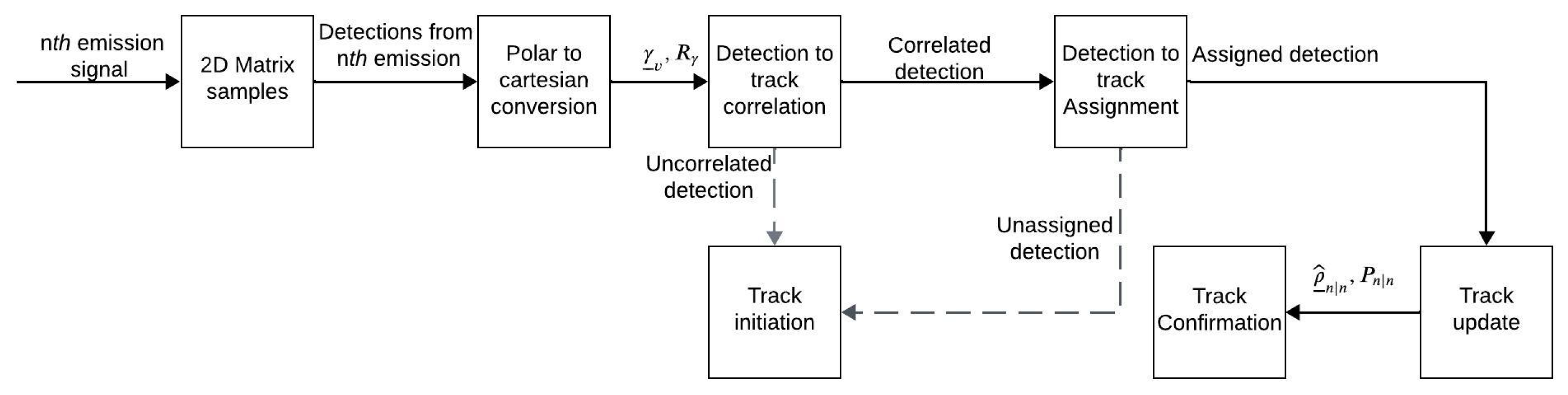
According to the block diagram in Figure 2, our target detection involves four steps: (1) pulse compression using a matched filter, (2) beamforming of U spatial domain beams and the formation of an angle–distance 2D matrix, (3) application of a constant 2D false alarm rate (CFAR) detector, and (4) binary map extraction and blob detection.
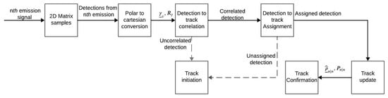
Figure 2.
A block diagram of the proposed detection and tracking scheme.
4.1. Forming the 2D Angle–Distance Matrix
For each emission of chirp signals, we create a 2D angle–distance matrix from the received reflections. The procedure for creating these matrices is as follows. First, a buffer of length is extracted at each of the array elements. Multiplying by half the speed of sound reflects the maximum detection range of the system. The received buffer is filtered separately at the output of each hydrophone with a matched filter that is adapted to the transmitted chirp signal. The compressed signals are beamformed into beams using the delay-and-sum procedure [38]. Formally, for a beam azimuth , the associated delay is . The data after beamforming for a reflection received at time instance , , is given by
The angle–distance matrix is obtained by
4.2. Blob Detection
The corresponding angle–distance 2D matrix I for each emission is filtered to reduce clutter. The detection threshold is calculated using a 2D CFAR detector to obtain a binary matrix of samples that passed (‘1’) or didn’t pass (‘0’) the threshold. The process involves estimation of the 2D angle- distance sample distribution parameters to calculate the CFAR detection threshold. The Rayleigh distribution,
where is the law-specific parameter, is adopted to model the clutter distribution [37]. The parameter is estimated by the maximum- likelihood [39]
where stands for the group of samples surrounding the sample under test in I that belong to the reference region. The CFAR threshold is given by
where is a target probability of false alarm.
The CFAR detection binary map is obtained by
We then join the regions in blobs to identify in B several regions of interest (ROIs) whihc contain potential targets and that form a connected region. For this purpose, we use the 4-connectivity method [40]. Higher-dimensional connectivity may improve the estimate of the center of mass of the blob, but the change is expected to be small (on the order of a few centimeters), which is also smoothed by the filtering. The range and the azimuth of the l-th blob is estimated by
where is the v-th coordinate of the center of mass of the l-th blob and is the sampling frequency. The azimuth is given by
If the number of elements in the acoustic array is small, the beamwidth is large. As a result, the beamforming grating lobes are also large, and a target can be received at adjacent beams. To deal with this ambiguity, we merge blobs that are closely spaced. Let be the group of all blobs obtained from a single emission. Let , be two separate blobs that are merged when
where and are the merging thresholds in range and azimuth, respectively. The threshold in range can be obtained by knowing the expected size of the mobile target to be detected, and the threshold in azimuth can be set by the position of the grating lobes of the array. The range and azimuth of the i-th merged blob at emission number n are given by
where is the group of all blobs that fulfill the conditions in (12). A tracking process is now applied to the merged blobs to detect a mobile target with a nearly constant velocity dynamical model. To make the tracking process efficient and with low complexity, we use a linear Kalman filter with a debiased polar to Cartesian measurement conversion as a fast and efficient method to handle a nonlinear measurement model.
4.3. Polar to Cartesian Conversion
Following [7] we convert the polar measurements () into a Cartesian space. The covariance matrix of the polar measurement noise is
where and are the standard deviations of the range and azimuth measurements. The debiased converted measurement in Cartesian coordinates is given by [7]
5. Underwater Target Tracking
The final step in our target detection is tracking, where we confirm valid mobile targets by detected blobs that follow a constant velocity dynamic model. The dynamic model is given by
where ; and are the position vectors of a target in the Cartesian X and Y frames; , are the Cartesian velocities; and is the process noise. The matrix A in (16) is given by
the matrix G is given by
and is the time of the n-th blob.
The measurement equation is given by
with
and is the measurement noise. The goal of our tracking is to estimate the position and velocity trajectories of a target. For this, we use Kalman filtering. The predicted step of the state vector and its covariance for the k-th track are given by
where is the process noise covariance matrix.
The update stage of the state vector and its covariance matrix is given by
where
and . The term is the covariance of the debiased converted measurement noise [37].
5.1. Detection to Track Correlation
To decrease computation time, we first apply a coarse gating between tracks and blobs that originate from one emission. Formally, only a blob that fulfills the following two conditions with at least one track is allowed; otherwise, a new track is created. The gating between the i-th blob and the k-th track in range and azimuth is given by
where and are the gating thresholds in range and azimuth, respectively. These thresholds can be determined using knowledge of the maximum speed of the mobile target and the time between adjacent emissions. The terms , and , are the Cartesian coordinates of the k-th track for emission number . Only tracks and blobs that meet constraint (24) are considered for the correlation
The result is further thresholded,
to ensure that a correct blob lies within the gate with a certain probability, which in turn is a function of the gate threshold . Blobs that are not correlated with any track are initiated as a new track. Correlated blobs are further considered for a detection to track assignment.
5.2. Detection to Track Assignment
For each chirp emission, the global assignment process determines the best association of blobs and tracks. Let be the association matrix, where and are the number of tracks and blobs, respectively, at emission number n. is given by
Let Y be a set of tracks and blobs that contain indices for possible assignments. The global assignment is obtained by finding the blobs–tracks assignment with the minimum global statistical distance, namely
To solve (28), we use the auction algorithm [41] due to its simplicity and low computational load. A blob that is not assigned to a track (in the case ) opens a new track. A track is removed if it has not been assigned to a blob at least times during the last emissions.
5.3. Track Confirmation
A track is confirmed if the number of blobs assigned to it is greater than . Formally,
where is an indicator function that is 1 if the argument is true and 0 otherwise.
5.4. Complexity Analysis
The complexity of our detection and tracking method for a single emission is
This is composed of a complexity of for the debiased Kalman filter [42], where is the size of the state vector , and stands for the 2D CFAR detection. The complexity of the particle filter is , and the complexity of the PHD filter is [43]. In a noisy environment, , which means that the proposed detection and tracking method has much lower complexity compared to the particle and PHD filters.
6. Performance Evaluation
In this section, we analyze the performance of our detection and tracking algorithm on both stimulative and real-world data. We compare our method with four benchmarks that focus on underwater acoustic detection and tracking. In particular, the methods in [44], hereafter referred to as Lo, and the scheme in [45], hereafter referred to as Karoui, are commonly used underwater detection and tracking schemes specifically designed for a high-clutter underwater environment. We also consider the methods in [13,32], hereafter referred to as Zhou and Kou. These are recent solutions for underwater tracking that aim to deal with the complexity of the environment and overlapping and interfering tracks, respectively.
The waveform is a linear chirp signal with a bandwidth of 10 kHz and a duration of 0.01 s. The sampling frequency is set to 50 kHz. The merging thresholds and are set to 10 m and , respectively. The standard deviations for the range and azimuth and are set to 0.3 m and , respectively. The standard deviation of the process noise is set to . The gating thresholds for range and azimuth, and , are set to 10 m and , respectively, and the threshold value for gating, , is set to 0.1. The threshold value for the track confirmation is set to . The track is deleted if the number of unassigned blobs exceeds 7 during 15 signal emissions.
6.1. Results on Simulated Data
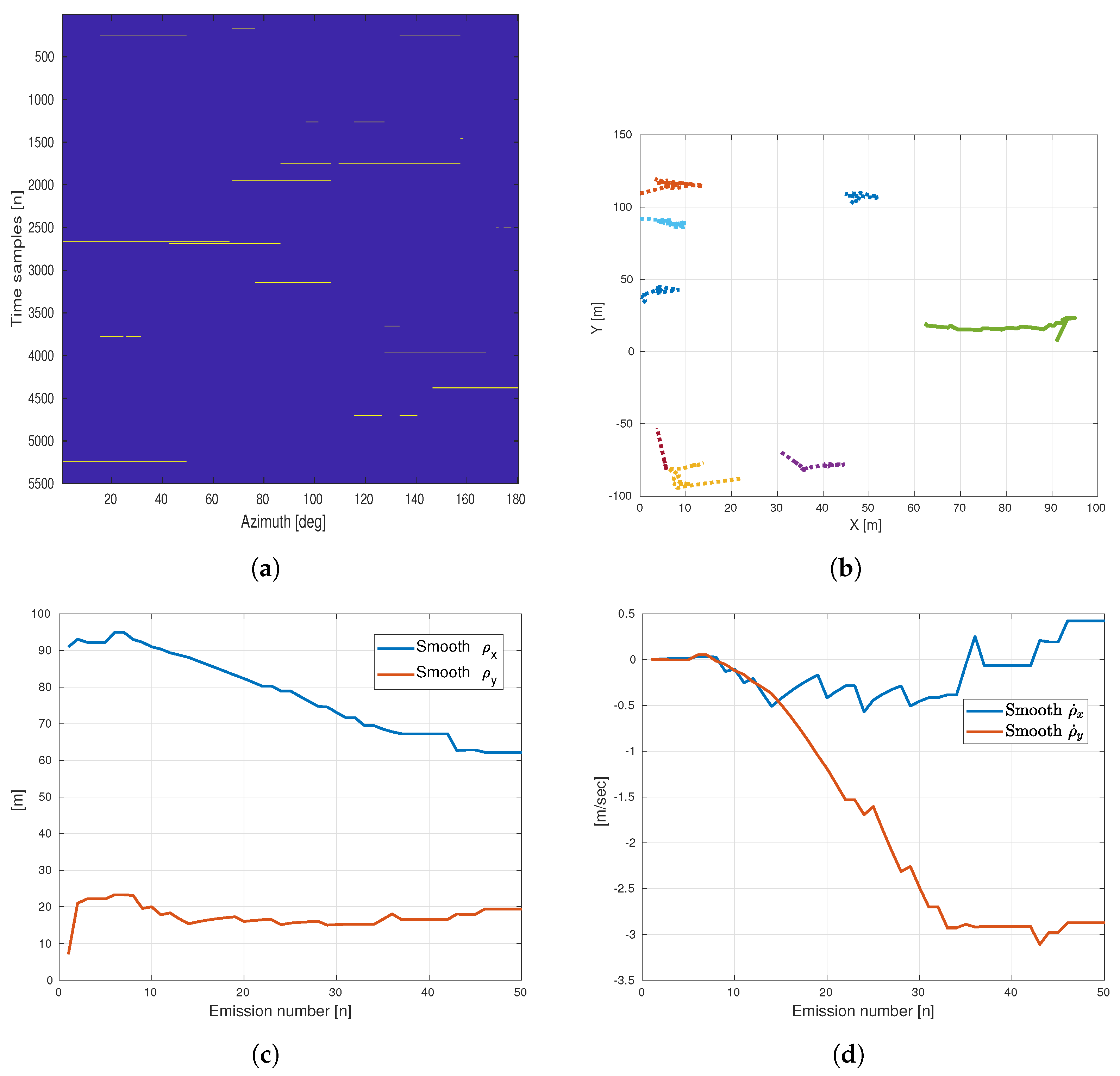
We simulate a single target with an initial position of m and m and a velocity of m/s and m/s. An example of the detection and tracking results can be found in Figure 3. The binary map is shown in Figure 3a, where the yellow regions indicate the detected blobs. Figure 3b shows the track map. The solid line indicates the track that belongs to the real target, and the dotted lines represent the false tracks. Figure 3c,d show the position and velocity estimation of the target, respectively. As long as the target is large enough for the wavelength of the emitted signal (about 5 cm), the size of the target has little effect on the performance. However, speed does have an impact on the tracking. We observe a convergence of velocity after 32 emissions. Figure 4 shows an example of the samples received from the emission after beamforming. The target is marked with the arrow, and the SCR is 3 dB.
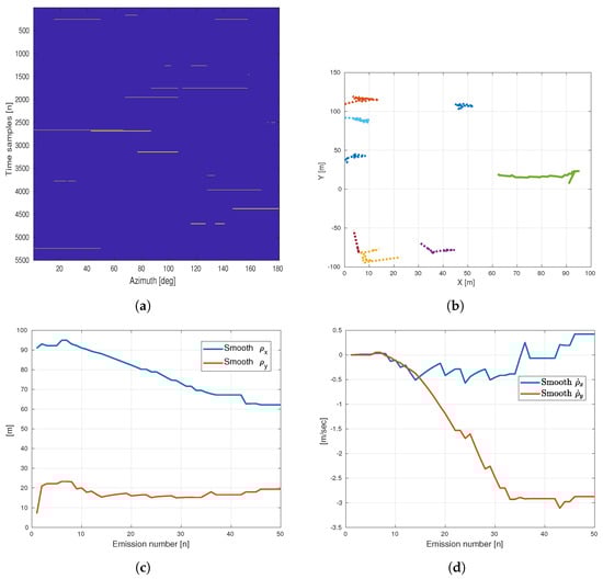
Figure 3.
Example of detection and tracking results. (a) The binary map B. Blobs are marked with yellow color. (b) Results of the tracking map. The dotted lines represent the false track, and the solid line represents the true track. (c) Position estimation of the true track. (d) Velocity estimation of the true track.
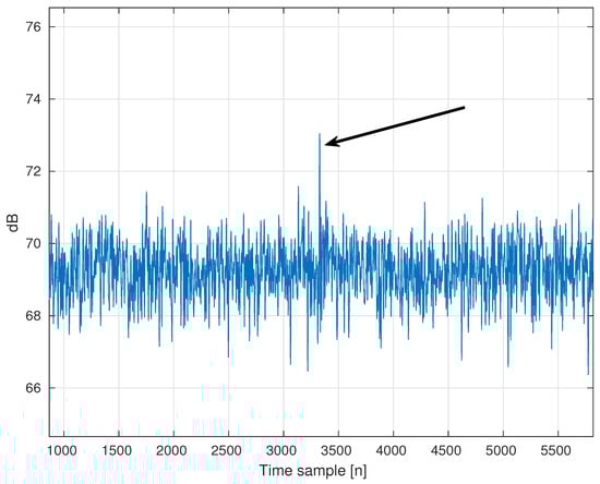
Figure 4.
An example of data samples after beamforming. The target is marked with the arrow.
6.1.1. Comparison with the Benchmarks
In this section, we compare the performance of our detection and tracking method with the above four benchmarks. As a performance metric, we consider the continuity of the estimated track. This is the ratio between the duration of the track and the lifetime of the target. A track continuity equal to ‘1’ would mean that the target is detected and continuously tracked for all signal emissions. We focus on the metric of track continuity because it includes both the location error (e.g., the root mean square error) and the tracking error (e.g., the ID switch). In particular, our definition of track continuity takes into account errors in the location of the target, where the continuity score decreases the farther the track is from the true location. The track continuity metric also directly quantifies our main goal of finding valid targets and characterizing their dynamics, rather than providing a true location estimate.
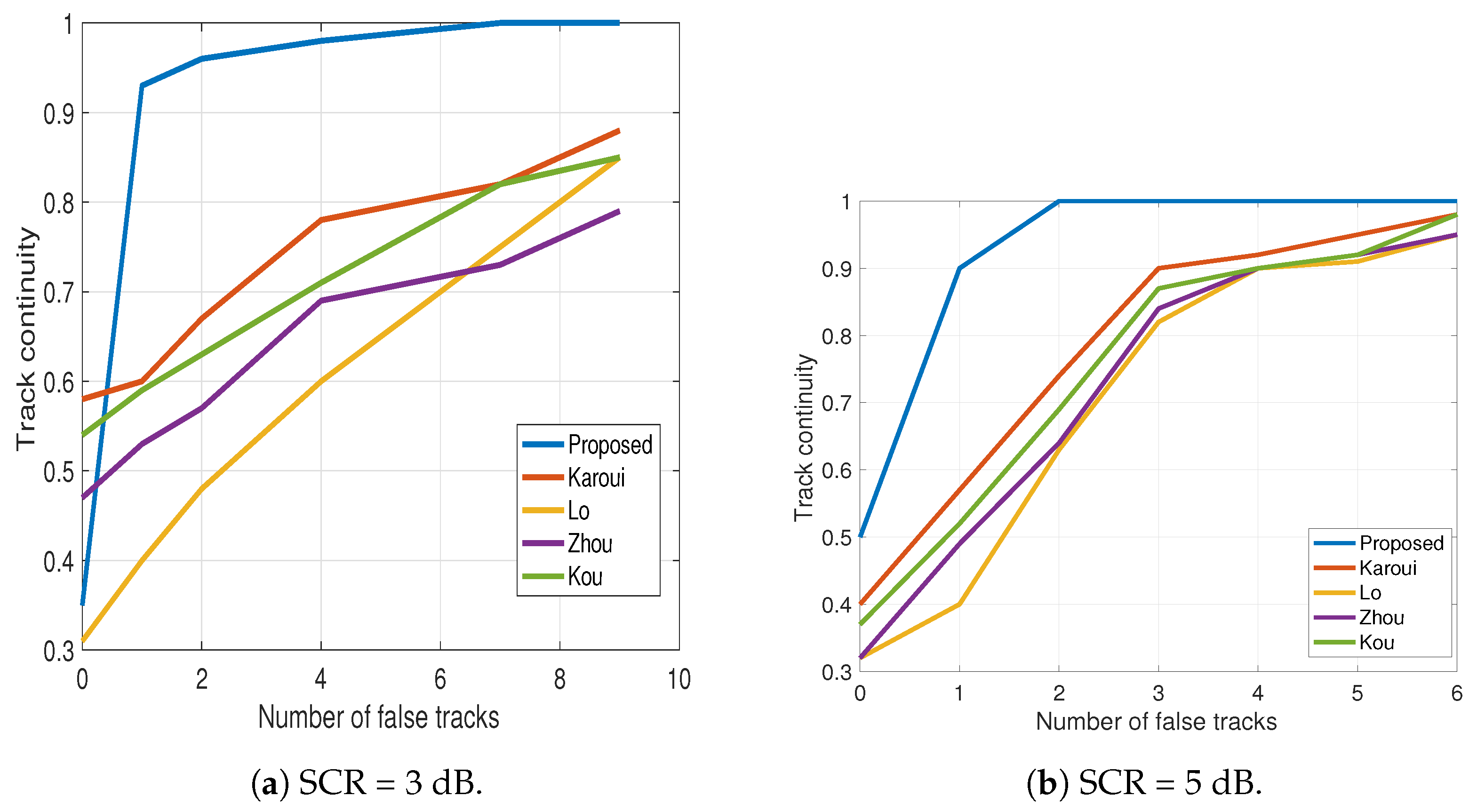
The results are shown for an SCR of 3 dB in Figure 5a and for an SCR of 5 dB in Figure 5b. We note that the results of Lo show the lowest track continuity. This is because this scheme does not merge closely spaced detections, which increases the false alarm rate and thus decreases the track continuity. We find that our method outperforms the benchmark for both tested SCR values and achieves a track continuity of more than 0.9 with less than two false traces. We find that the SCR has an impact on the tracking performance. For an SCR of 3 dB, our method achieves a track continuity of one with seven false tracks, while, for SCR of 5 dB, the same tracking continuity is achieved with two false tracks.
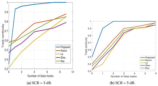
Figure 5.
Track continuity vs. the number of false tracks to compare sensitivity to the detection threshold. Results shown for two SCR values.
A comparison of the runtime of our proposed approach with that of four benchmarks (see Section 6) can be found in Table 1. The runtime was measured on a Raspberry Pi 0 Type 2 processor (500 MB RAM and a dual-core), which is the platform used in our sea experiments below. A considerable improvement in runtime was observed for our proposed scheme at the cost of an increase in the memory usage.

Table 1.
Runtime and memory usage for the proposed approach and the three benchmark schemes over a Raspberry Pi 0 Type 2 processor. The algorithms were tested for acoustic reflections from emissions spaced by 100 ms of a 10 ms long linear chirp signal in the frequency band 30 kHz–40 kHz. The scenario includes one simulated target.
6.1.2. Confirmation of Threshold Analysis
In this section, we analyze the continuity of the tracks and the number of false tracks for different values of the track confirmation thresholds, . In this analysis, we set the detection threshold to 0.2 and the SCR to 3 dB. The results are shown in Figure 6. When the confirmation threshold is small, more tracks are validated, and the number of false tracks increases. However, the track associated with the true target is reported with less validation time. When the confirmation threshold is high, the validation time is also high, and consequently the number of false tracks decreases, but the track associated with the true target is reported with a higher latency. As expected, increasing the confirmation threshold does not affect the continuity of the tracks but rather reduces the number of false tracks.
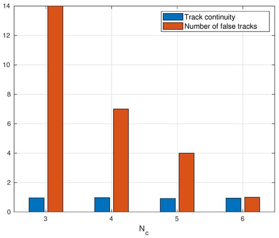
Figure 6.
Track continuity and number of false tracks obtained for different values of . The results were obtained for SCR = 3 dB and .
6.2. Sea Trial Results
6.2.1. Experimental Setup
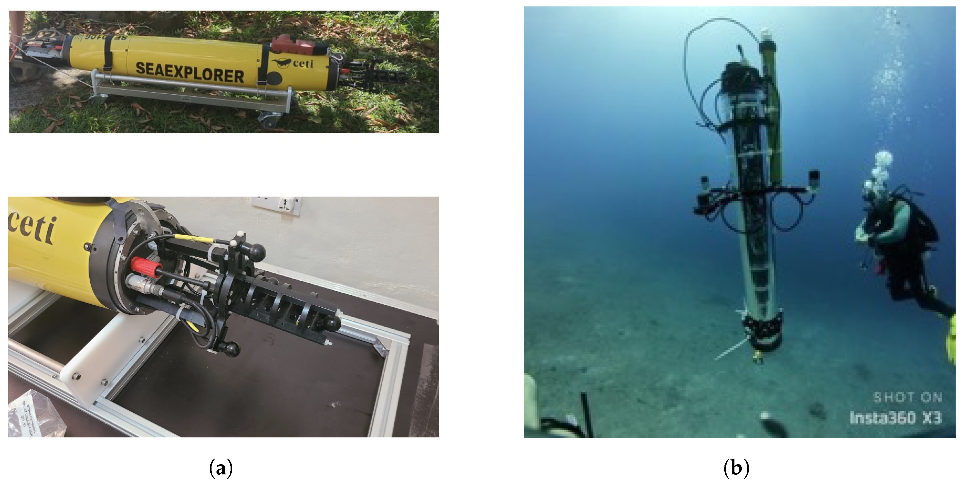
To further validate the performance of our proposed detection and tracking method, we now present the results of a designated sea experiment conducted in Šibenik, Croatia, in January 2024. The experiment involved a self-built floater with a self-built, simultaneously sampled, four hydrophone planar array and a self-built single projector (see Figure 7a). The hydrophones and the projector were piezoelectric, self-potted and calibrated in a testing pool using an IC-listen recorder as reference. During calibration, short CW pulses were sent to separate the direct path from the reflections in the pool. The hydrophones were mounted on the floater using a rigid holder with an aperture of 25 cm apart. The projector was positioned in the center of the holder about 40 cm above the hydrophones. A compass was integrated into the system to provide yaw measurements for each emission.
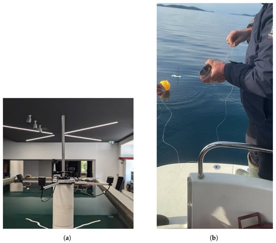
Figure 7.
Pictures from the sea experiment. (a) The 4-element hydrophone array with the projector positioned above it. (b) A picture of one of the tested fish. The GPS and the surface float attached to it can be seen in the water. Hydrophones and projectors are installed above the floater’s body to reduce interference.
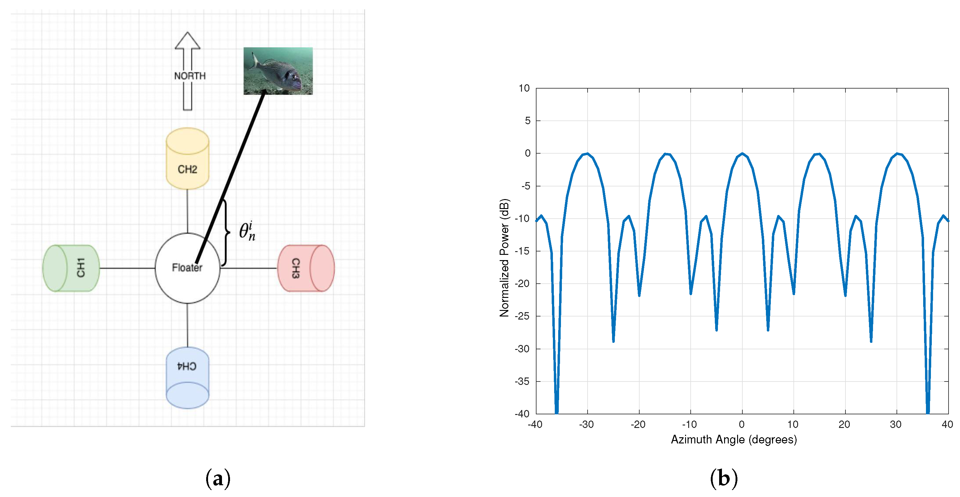
The measurements of all elements to a reference point on the floater were fed into the multidimensional scaling (MDS) algorithm [46] to obtain a 3D estimate of the position of the array. A schematic representation of our system can be found in Figure 8a, where the hydrophones are labeled ch1 to ch4. The positions of ch1, ch2, ch3, and ch4 are (−38.5, 0), (0, 39.5), (40.5, 0), and (0, −40.5), respectively. The effective beam pattern of this constellation is shown in Figure 8b. The figure shows that due to the small array and small aperture resulting from the limitations of the floater platform, large ambiguities occur in the azimuth cut. The beamwidth is about 5 degrees (3 dB beam), but the spatial attenuation due to beamforming is at most 25 dB. This means that a large reflector can distract the detector from the actual target, and multiple targets can be displayed as interrupted tracks.

Figure 8.
Scheme of the hydrophone array tested during the sea experiment. (a) A scheme of our platform with four hydrophones. (b) Beam pattern in azimuth cut of the array.
In our experiment, the floater was set so that it autonomously maintained a depth of 20 m with 1 m overshoot and the water depth was about 30 m. The position of the floater was monitored by attaching it to a small surface buoy with a GPS logger (2 m accuracy). An alternative is to localize the fish using acoustic tags so that the fish do not have to be tied to the small buoys. However, the signal generation rate of such tags is at best in the order of a few tens of seconds (cf. [47]), while a rate of less than one second is required to track the trajectory given the mobility of the fish. The sea was calm, the bathymetry was approximately flat, and the seabed consisted mainly of muddy sediment. The sound speed profile was 1500 m/s in the first 3 m, due to a freshwater layer from the Krka River, and was fixed at 1520 m/s below this layer. The emitted signals were 10 ms linear frequency modulated chirps in the frequency band of 30 kHz–40 kHz. A guard interval of 1 s between adjacent emissions was used to suppress inter-pulse interference, while the maximum distance for creating the distance–angle 2D matrices was set to 100 m. The sampling rate was set to 96 k samples per second with 2 bytes per sample.
We experimented with six gilt-head seabream as the target fish. The fish were released near the floater buoy and swam freely away from it. To obtain ground truth on the location of the fish, the fish were attached with a 20 m fishing line to a foam-based float, on which we attached a GPS logger (±2 m accuracy). See the illustration in Figure 9. Due to the length of the fishing line and the inaccuracies of the GPS position, the inaccuracy of the true position of the fish is at most 24 m. Three experiments were carried out: Exp 1: Release of a single fish; Exp 2: Release of two fish simultaneously; and Exp 3: Release of three fish simultaneously. We note that in Exp 1 and Exp 2, the fish swam in different directions, while in Exp 3, the trajectories of the fish crossed. In each experiment, five tracking sessions were measured in each experiment by moving the floater close to the location of the released fish. We confirm that ethical approval for this experiment was obtained from the Ruđer Bošković Institute, Croatia, and the experiments were conducted in accordance with the approved guidelines and EU ethical regulations. The methods used followed the ARRIVE guidelines.
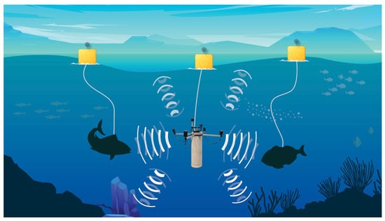
Figure 9.
Illustration of the scenario tested in the sea experiments.
6.2.2. Experiment Results
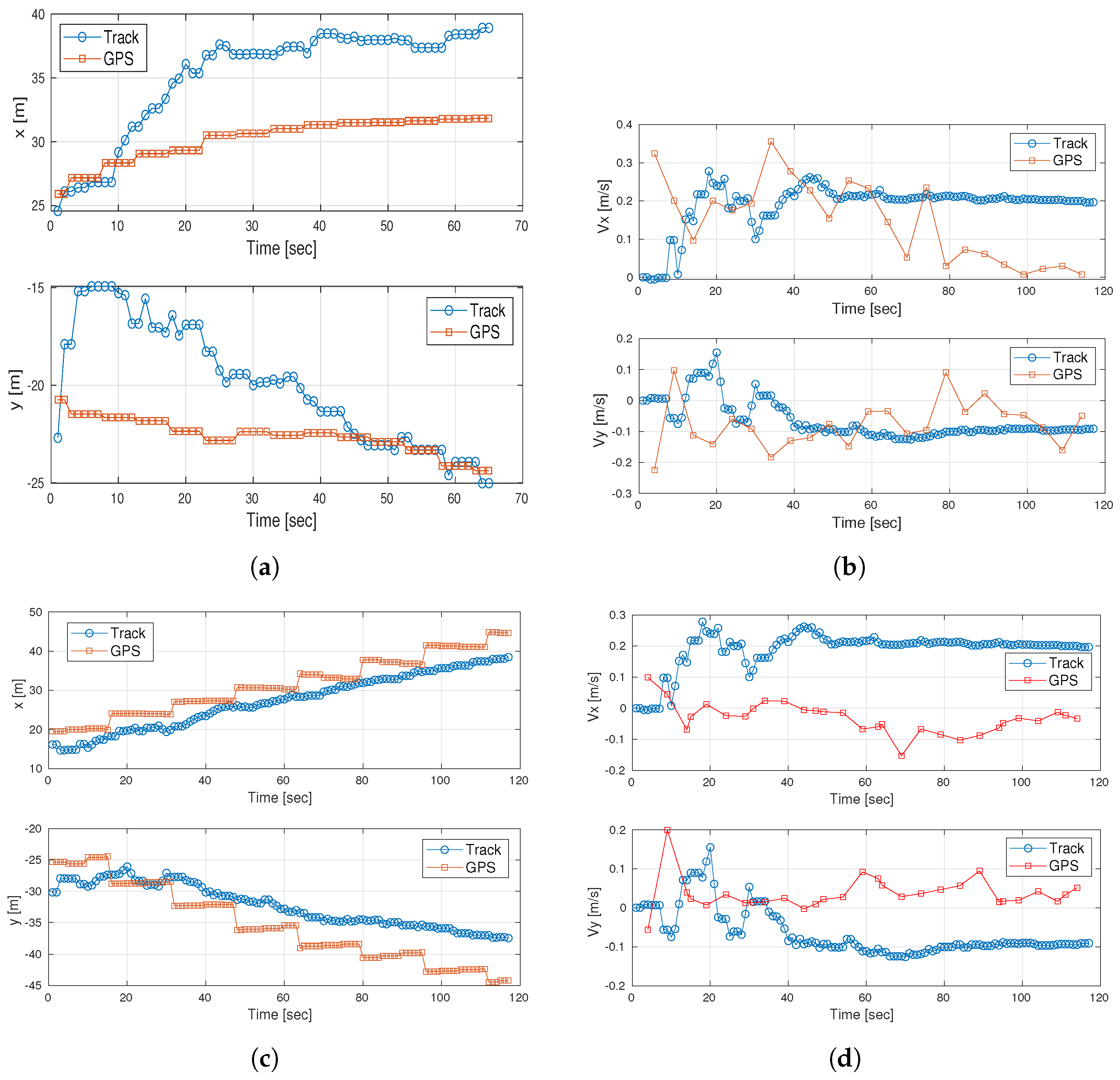
Examples of the tracks obtained with our proposed scheme in one of the sessions of Exp 2 are shown in Figure 10. We show the results with respect to the GPS track over a duration of 120 s in terms of horizontal location (axis x and y) and speed (axis x and y). Based on the results, we observe a different swimming behavior of the two fish, with fish #2 swimming faster and more smoothly. The two fish in Exp 2 swam in different directions but at approximately the same speed. We note that the results of our tracking method are close to the GPS ground truth data, where the error was below the maximum ambiguity in both cases. For fish #1, the convergence of position was achieved after 45 s, and the error in velocity estimation was about 0.2 m/s in both coordinates. The convergence of the position of fish #2 was achieved after 10 s and the velocity error was 0.2 m/s and 0.1 m/s for the X and Y coordinates, respectively.
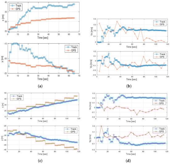
Figure 10.
Track results versus GPS ground truth data. Results are shown for the X-Y coordinates. (a) Exp 2: track of horizontal location of fish #1. (b) Exp 2: track of speed of fish #1. (c) Exp 2: track of horizontal location of fish #2. (d) Exp 2: track of speed of fish #2.
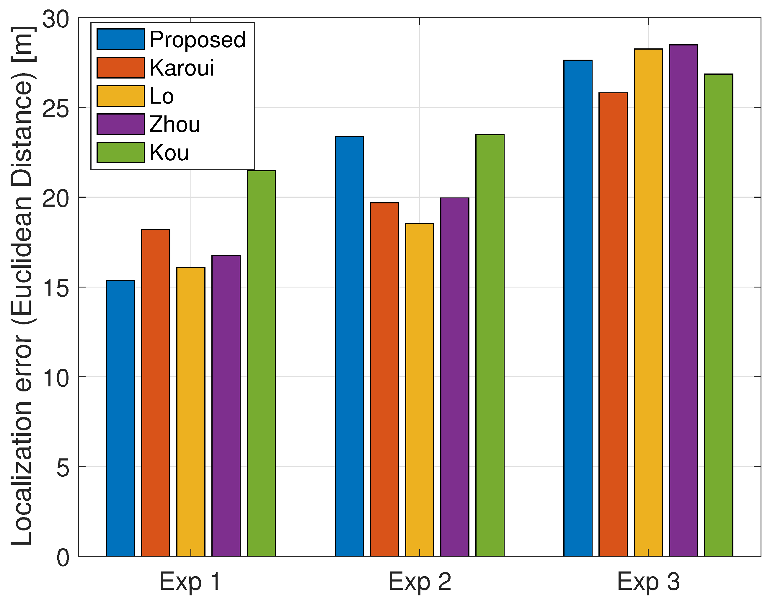
The results in terms of the Euclidean distance to the GPS ground truth measurements across all experimental sessions are shown in Figure 11 for . Here, only the true tracks are considered, and the localization error is calculated as an average across the track of observations. We find that the Euclidean error remains roughly the same between Exp 1 and Exp 2, while the error increases at Exp 3. This is because in the latter, the fish crossed each other, resulting in track intersections. There is no significant advantage for any of the explored methods, as only valid tracks were considered.

Figure 11.
Average localization error across valid tracks. Results averaged per experiment for all 5 sessions. . The error in the true position of the fish is at most 24 m.
Figure 12 presents a comparison of the track continuity for the sea trial results between our method and the four explored benchmarks. The track was associated with the true fish in the sea trial by the GPS data. As for the false detection, there could be other valid targets besides the tagged fish. Thus, with no ground truth information for the number of false tracks, we measure the track continuity for different detection thresholds by changing the target false alarm rate as defined in (8). The results confirm our observations from the simulations in Figure 5. Higher track continuity is observed for our proposed approach with robustness to the choice of threshold.
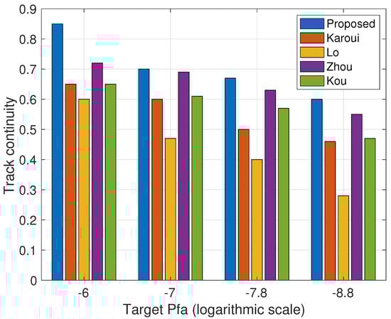
Figure 12.
Track continuity obtained for a detection threshold set by changing the target values according to (8). Results averaged over all experiment sessions for .
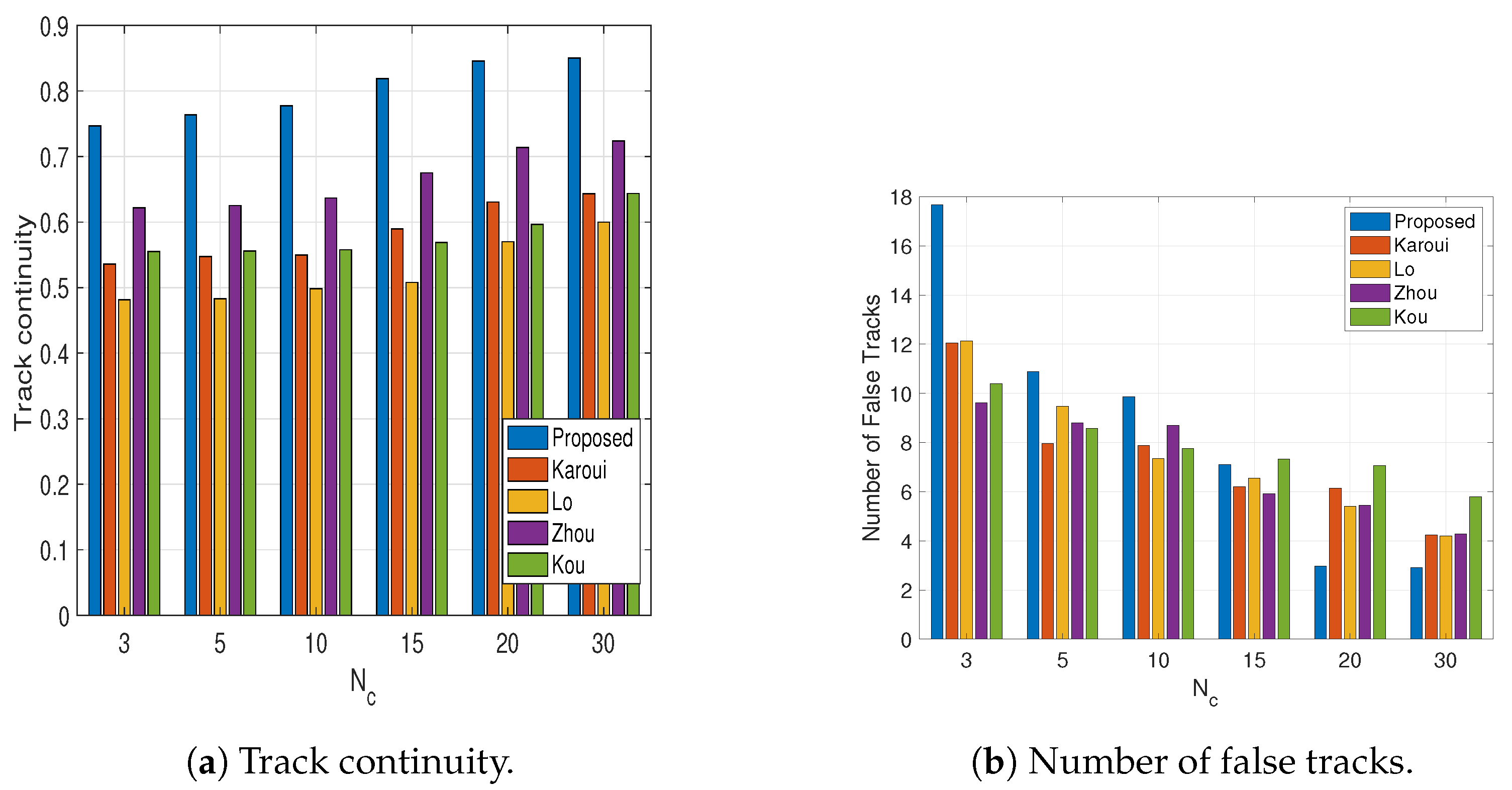
For the choice of , the continuity of the tracks and the number of false tracks as a function of the observation window are shown in the top and bottom panels of Figure 13, respectively. For both metrics, we find that our proposed solution converges after , which reflects on the robustness of the solution. No convergence is observed for the benchmarks. For all benchmarks, the track continuity seems to be insensitive to the value of . However, a strong dependence on the number of false tracks is observed. Similar to Figure 6, our proposed solution starts with a very high number of false tracks, which quickly decreases as more observations are collected.
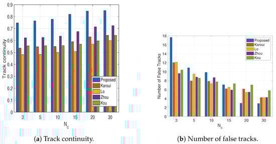
Figure 13.
Track continuity (left panel) and number of false tracks (right panel) as a function of the number of emissions, . Target . Results averaged over all experiment sessions.
7. Conclusions
We have presented a method for detecting and tracking mobile underwater targets for biodiversity assessment. The problem considered focuses on accurate estimation of the number of valid tracks rather than localization. That is, a high ratio between the duration of the track and the lifetime of the target is required. To overcome the challenge of false tracking, we developed a tracking mechanism that clusters sets of binary maps and performs tracking on blobs rather than individual detection. An adaptive threshold manages the high and time-varying clutter. With a real-time application in mind, we developed a tracking solution with low complexity. The results from the simulated data show that our method effectively reduces the number of false tracks while maintaining high tracking continuity and achieving better performance than four benchmark schemes. It is shown that the tracking is stable with small number of false tracks even with a low signal-to-clutter ratio. The results were confirmed in a sea experiment in the Adriatic Sea, where a float with a projector and four rigidly mounted hydrophones was used to track up to three simultaneously free-moving fish. Although our method is capable of tracking multiple targets simultaneously, it is sensitive to occlusions when targets cross each other, and to track discontinuities when a target rapidly changes its speed. Further work will therefore extend this work to address the spatial ambiguity of the array and utilize the multiple arrivals reflected from the mobile target for improved tracking.
Author Contributions
Conceptualization, R.D.; methodology, A.A. and R.D.; software, A.A. and R.D.; validation, N.M.; formal analysis, A.A. and R.D.; investigation, A.A.; resources, N.C., N.M. and R.D.; data curation, A.A. and N.C.; writing—review and editing, A.A. and R.D.; visualization, A.A.; supervision, R.D.; project administration, N.M. and R.D.; funding acquisition, N.M. and R.D. All authors have read and agreed to the published version of the manuscript.
Funding
This work was sponsored in part by the Schmidt Marine Foundation via the Global Fisheries Tech Initiative, and by the European Union’s Horizon Europe programme under the UWIN-LABUST project (project no. 101086340), and by Project CETI via grants from Dalio Philanthroies and Ocean X; Sea Grape Foundation; Rosamund Zander/Hansjorg Wyss, Chris Anderson/Jacqueline Novogratz through The Audacious Project: a collaborative funding initiative housed at TED.
Data Availability Statement
No data is assosiated with this research.
Conflicts of Interest
The authors declare no conflicts of interest. The funders had no role in the design of the study; in the collection, analyses, or interpretation of data; in the writing of the manuscript, or in the decision to publish the results.
References
- De La Torre, P.R.; Smith, E.L.; Sancheti, A.; Salama, K.N.; Berumen, M.L. iSAT: The mega-fauna acoustic tracking system. In Proceedings of the 2013 MTS/IEEE OCEANS, Bergen, Norway, 10–14 June 2013; pp. 1–6. [Google Scholar]
- Park, J.; Kim, G.; Seok, J.; Hong, J. Pulsed Active Sonar Using Generalized Sinusoidal Frequency Modulation for High-Speed Underwater Target Detection and Tracking. IEEE Access 2023, 11, 143081–143091. [Google Scholar] [CrossRef]
- Andreas, J.; Beguš, G.; Bronstein, M.M.; Diamant, R.; Delaney, D.; Gero, S.; Goldwasser, S.; Gruber, D.F.; de Haas, S.; Malkin, P.; et al. Toward understanding the communication in sperm whales. iScience 2022, 25, 104393. [Google Scholar] [CrossRef]
- Rautureau, C.; Goulon, C.; Guillard, J. In situ TS detections using two generations of echo-sounder, EK60 and EK80: The continuity of fishery acoustic data in lakes. Fish. Res. 2022, 249, 106237. [Google Scholar] [CrossRef]
- Ferguson, B. Improved time-delay estimates of underwater acoustic signals using beamforming and prefiltering techniques. IEEE J. Ocean. Eng. 1989, 14, 238–244. [Google Scholar] [CrossRef]
- Dubrovinskaya, E.; Kebkal, V.; Kebkal, O.; Kebkal, K.; Casari, P. Underwater Localization via Wideband Direction-of-Arrival Estimation Using Acoustic Arrays of Arbitrary Shape. Sensors 2020, 20, 3862. [Google Scholar] [CrossRef] [PubMed]
- Lerro, D.; Bar-Shalom, Y. Tracking with debiased consistent converted measurements versus EKF. IEEE Trans. Aerosp. Electron. Syst. 1993, 29, 1015–1022. [Google Scholar] [CrossRef]
- Blackman, S.S.; Popoli, R. Design and Analysis of Modern Tracking Systems; Artech House: Norwood, MA, USA, 1999. [Google Scholar]
- Kalyan, B.; Balasuriya, A. Sonar based automatic target detection scheme for underwater environments using CFAR techniques: A comparative study. In Proceedings of the 2004 International Symposium on Underwater Technology (IEEE Cat. No.04EX869), Taipei, Taiwan, 20–23 April 2004; pp. 33–37. [Google Scholar]
- Blum, R.; Kassam, S. Distributed cell-averaging CFAR detection in dependent sensors. IEEE Trans. Inf. Theory 1995, 41, 513–518. [Google Scholar] [CrossRef]
- Acosta, G.G.; Villar, S.A. Accumulated CA–CFAR Process in 2-D for Online Object Detection From Sidescan Sonar Data. IEEE J. Ocean. Eng. 2015, 40, 558–569. [Google Scholar] [CrossRef]
- Rohling, H. Ordered statistic CFAR technique - an overview. In Proceedings of the 2011 12th International Radar Symposium (IRS), Leipzig, Germany, 7–9 September 2011; pp. 631–638. [Google Scholar]
- Zhou, T.; Si, J.; Wang, L.; Xu, C.; Yu, X. Automatic Detection of Underwater Small Targets Using Forward-Looking Sonar Images. IEEE Trans. Geosci. Remote Sens. 2022, 60, 4207912. [Google Scholar] [CrossRef]
- Zhan, D.; Zheng, H.; Xu, W. Tracking Control of Autonomous Underwater Vehicles with Acoustic Localization and Extended Kalman Filter. Appl. Sci. 2021, 11, 8038. [Google Scholar] [CrossRef]
- Kumar, M.; Mondal, S. Recent developments on target tracking problems: A review. Ocean Eng. 2021, 236, 109558. [Google Scholar] [CrossRef]
- Kim, J. Hybrid TOA–DOA techniques for maneuvering underwater target tracking using the sensor nodes on the sea surface. Ocean Eng. 2021, 242, 110110. [Google Scholar] [CrossRef]
- Kazimierski, W.; Zaniewicz, G. Determination of process noise for underwater target tracking with forward looking sonar. Remote Sens. 2021, 13, 1014. [Google Scholar] [CrossRef]
- Kumar, D.R. Hybrid unscented Kalman filter with rare features for underwater target tracking using passive sonar measurements. Optik 2021, 226, 165813. [Google Scholar] [CrossRef]
- Khan, A.; Fouda, M.M.; Do, D.T.; Almaleh, A.; Alqahtani, A.M.; Rahman, A.U. Underwater target detection using deep learning: Methodologies, challenges, applications, and future evolution. IEEE Access 2024, 12, 12618–12635. [Google Scholar] [CrossRef]
- Bar-Shalom, Y.; Kirubarajan, T.; Lin, X. Probabilistic data association techniques for target tracking with applications to sonar, radar and EO sensors. IEEE Aerosp. Electron. Syst. Mag. 2005, 20, 37–56. [Google Scholar] [CrossRef]
- Clark, D.; Vo, B.N.; Bell, J. GM-PHD filter multitarget tracking in sonar images. In Signal Processing, Sensor Fusion, and Target Recognition XV; Kadar, I., Ed.; International Society for Optics and Photonics, SPIE: Pune, India, 2006; Volume 6235, p. 62350R. [Google Scholar]
- Zhou, T.; Wang, Y.; Zhang, L.; Chen, B.; Yu, X. Underwater multitarget tracking method based on threshold segmentation. IEEE J. Ocean. Eng. 2023, 48, 1255–1269. [Google Scholar] [CrossRef]
- Zhou, T.; Wang, Y.; Chen, B.; Zhu, J.; Yu, X. Underwater Multitarget Tracking With Sonar Images Using Thresholded Sequential Monte Carlo Probability Hypothesis Density Algorithm. IEEE Geosci. Remote Sens. Lett. 2022, 19, 1–5. [Google Scholar] [CrossRef]
- Li, M.; Ji, H.; Wang, X.; Weng, L.; Gong, Z. Underwater object detection and tracking based on multi-beam sonar image processing. In Proceedings of the 2013 IEEE International Conerence on Robotics and Biomimetics (ROBIO), Shenzhen, China, 12–14 December 2013; pp. 1071–1076. [Google Scholar]
- Georgescu, R.; Willett, P. The GM-CPHD Tracker Applied to Real and Realistic Multistatic Sonar Data Sets. IEEE J. Ocean. Eng. 2012, 37, 220–235. [Google Scholar] [CrossRef]
- Georgescu, R.; Schoenecker, S.; Willett, P. GM-CPHD and MLPDA applied to the SEABAR07 and TNO-blind multi-static sonar data. In Proceedings of the 2009 12th International Conference on Information Fusion, Seattle, WA, USA, 6–9 July 2009; pp. 1851–1858. [Google Scholar]
- Blanding, W.R.; Willett, P.K.; Bar-Shalom, Y.; Lynch, R.S. Directed subspace search ML-PDA with application to active sonar tracking. IEEE Trans. Aerosp. Electron. Syst. 2008, 44, 201–216. [Google Scholar] [CrossRef]
- Luo, J.; Han, Y.; Fan, L. Underwater acoustic target tracking: A review. Sensors 2018, 18, 112. [Google Scholar] [CrossRef] [PubMed]
- Mellema, G.R. Improved active sonar tracking in clutter using integrated feature data. IEEE J. Ocean. Eng. 2018, 45, 304–318. [Google Scholar] [CrossRef]
- He, X.; Wang, Y.; Yang, S. Gaussian mixture CBMeMBer filter for multi-target tracking with Non-Gaussian noise. IAENG Int. J. Appl. Math. 2022, 52, 1–8. [Google Scholar]
- Jahan, K.; Rao, S.K. Implementation of underwater target tracking techniques for Gaussian and non-Gaussian environments. Comput. Electr. Eng. 2020, 87, 106783. [Google Scholar] [CrossRef]
- Kou, K.; Li, B.; Ding, L.; Song, L. A distributed underwater multi-target tracking algorithm based on two-layer particle filter. J. Mar. Sci. Eng. 2023, 11, 858. [Google Scholar] [CrossRef]
- Yuan, Y.; Li, Y.; Liu, Z.; Chan, K.Y.; Zhu, S.; Guan, X. A three dimensional tracking scheme for underwater non-cooperative objects in mixed LOS and NLOS environment. Peer-to-Peer Netw. Appl. 2019, 12, 1369–1384. [Google Scholar] [CrossRef]
- WANG, Y.; LI, Y.; JU, D.; HUANG, H. A multi-target passive tracking algorithm based on unmanned underwater vehicle. J. Electron. Inf. Technol. 2020, 42, 2013–2020. [Google Scholar]
- Katz, Y.; Groper, M. On the Development of a Mid-Depth Lagrangian Float for Littoral Deployment. J. Mar. Sci. Eng. 2022, 10, 2030. [Google Scholar] [CrossRef]
- Babić, A.; Oreč, M.; Mišković, N.; Diamant, R. SOUND: A swarm of low-cost floaters for sustainable fishing. In Proceedings of the OCEANS 2024, Singapore, 15–18 April 2024; pp. 1–5. [Google Scholar]
- Quidu, I.; Jaulin, L.; Bertholom, A.; Dupas, Y. Robust Multitarget Tracking in Forward-Looking Sonar Image Sequences Using Navigational Data. IEEE J. Ocean. Eng. 2012, 37, 417–430. [Google Scholar] [CrossRef]
- Madanayake, A.; Wijenayake, C.; Wijayaratna, S.; Acosta, R.; Hariharan, S.I. 2-D-IIR Time-Delay-Sum Linear Aperture Arrays. IEEE Antennas Wirel. Propag. Lett. 2014, 13, 591–594. [Google Scholar] [CrossRef]
- Grieve, P. The optimum constant false alarm probability detector for relatively coherent multichannel signals in Gaussian noise of unknown power. IEEE Trans. Inf. Theory 1977, 23, 708–721. [Google Scholar] [CrossRef]
- Samet, H.; Tamminen, M. Efficient component labeling of images of arbitrary dimension represented by linear bintrees. IEEE Trans. Pattern Anal. Mach. Intell. 1988, 10, 579–586. [Google Scholar] [CrossRef]
- Bertsekas, D.P. Network Optimization; Athena Scientific: Belmont, MA, USA, 1998. [Google Scholar]
- Raitoharju, M.; Piché, R. On Computational Complexity Reduction Methods for Kalman Filter Extensions. IEEE Aerosp. Electron. Syst. Mag. 2019, 34, 2–19. [Google Scholar] [CrossRef]
- Cong, S.; Hong, L. Computational complexity analysis for multiple hypothesis tracking. In Proceedings of the 36th IEEE Conference on Decision and Control, San Diego, CA, USA, 12 December 1997; Volume 5, pp. 4991–4996. [Google Scholar]
- Lo, K.; Ferguson, B. Automatic detection and tracking of a small surface watercraft in shallow water using a high-frequency active sonar. IEEE Trans. Aerosp. Electron. Syst. 2004, 40, 1377–1388. [Google Scholar] [CrossRef]
- Karoui, I.; Quidu, I.; Legris, M. Automatic Sea-Surface Obstacle Detection and Tracking in Forward-Looking Sonar Image Sequences. IEEE Trans. Geosci. Remote Sens. 2015, 53, 4661–4669. [Google Scholar] [CrossRef]
- Wickelmaier, F. An Introduction to MDS; Sound Quality Research Unit, Aalborg University: Aalborg, Denmark, 2003; Volume 46, pp. 1–26. [Google Scholar]
- Alexandri, T.; Miller, E.; Spanier, E.; Diamant, R. Tracking the slipper lobster using acoustic tagging: Testbed description. IEEE J. Ocean. Eng. 2018, 45, 577–585. [Google Scholar] [CrossRef]


Disclaimer/Publisher’s Note: The statements, opinions and data contained in all publications are solely those of the individual author(s) and contributor(s) and not of MDPI and/or the editor(s). MDPI and/or the editor(s) disclaim responsibility for any injury to people or property resulting from any ideas, methods, instructions or products referred to in the content. |
© 2025 by the authors. Licensee MDPI, Basel, Switzerland. This article is an open access article distributed under the terms and conditions of the Creative Commons Attribution (CC BY) license (https://creativecommons.org/licenses/by/4.0/).