Multi-Sensor Fusion and Machine Learning for Forest Age Mapping in Southeastern Tibet

Abstract

Forest age is a key factor in determining the carbon sequestration capacity and trends of forests. Based on the Google Earth Engine platform and using the topographically complex and climatically diverse Southeastern Tibet as the study area, we propose a new method for forest age estimation that integrates multi-source remote-sensing data with machine learning. The study employs the Continuous Degradation Detection (CODED) algorithm combined with spectral unmixing models and Normalized Difference Fraction Index (NDFI) time series analysis to update forest disturbance information and provide annual forest distribution, mapping young forest distribution. For undisturbed forests, we compared 12 machine-learning models and selected the Random Forest model for age prediction. The input variables include multiscale satellite spectral bands (Sentinel-2 MSI, Landsat series, PROBA-V, MOD09A1), vegetation parameter products (canopy height, productivity), data from the Global Ecosystem Dynamics Investigation (GEDI), multi-band SAR data (C/L), vegetation indices (e.g., NDVI, LAI, FPAR), and environmental factors (climate seasonality, topography). The results indicate that the forests in Southeastern Tibet are predominantly overmature (>120 years), accounting for 87% of the total forest cover, while mature (80–120 years), sub-mature (60–80 years), intermediate-aged (40–60 years), and young forests (< 40 years) represent relatively lower proportions at 9%, 1%, 2%, and 1%, respectively. Forest age exhibits a moderate positive correlation with stem biomass (r = 0.54) and leaf-area index (r = 0.53), but weakly negatively correlated with L-band radar backscatter (HV polarization, r = −0.18). Significant differences in reflectance among different age groups are observed in the 500–1000 nm spectral band, with 100 m resolution PROBA-V data being the most suitable for age prediction. The Random Forest model achieved an overall accuracy of 62% on the independent validation set, with canopy height, L-band radar data, and temperature seasonality being the most important predictors. Compared with 11 other machine-learning models, the Random Forest model demonstrated higher accuracy and stability in estimating forest age under complex terrain and cloudy conditions. This study provides an expandable technical framework for forest age estimation in complex terrain areas, which is of significant scientific and practical value for sustainable forest resource management and global forest resource monitoring.

1. Introduction

Forest age is a critical parameter in forest ecosystems. Forest age significantly influences carbon sequestration capacity, biomass accumulation, ecological functions, and growth stages [1,2,3]. Accurate assessment of forest age is crucial for forest carbon cycle modeling, biodiversity conservation, forest management, and climate change mitigation [4,5]. Traditional forest survey methods, such as tree core sampling and estimations based on tree height and diameter at breast height, can provide relatively accurate forest age data at the sample scale, but they are destructive to trees and time-consuming [6]. Scaling up these methods for large-area applications is challenging due to low spatial and coarse temporal resolutions [7,8], which limits the ability to meet high spatiotemporal resolution demands in forest age mapping [9].

Advances in remote-sensing technology, both active and passive remote-sensing methods, have provided abundant data support for forest age estimation through both active and passive methods [10,11]. Forest spectral reflectivity exhibits significant phase-dependent characteristics with respect to forest age [12]. By analyzing spectral reflectance, canopy texture, light transmittance, and biomass from remote-sensing images, forest age can be indirectly estimated [13]. For instance, Kayitakire et al. (2006) used IKONOS-2 multispectral and panchromatic images (1 m resolution) to generate age-distribution maps of 7900 hectares of plantations in Eastern Belgium using linear regression methods [14]. Similarly, Tang et al. (2020) combined Sentinel-2 imagery with machine-learning models to achieve 10 m resolution age estimation for larch forests in Chifeng [15]. However, optical remote-sensing-based methods often suffer from saturation effects and limited model generalizability, particularly for mature and overripened forests [1,16,17].

Active remote-sensing technologies, such as Synthetic Aperture Radar (SAR) and Light Detection and Ranging (LiDAR), can partially overcome these limitations [18,19]. Structural characteristics of forests, such as height, gap distribution, and canopy roughness, vary significantly between early and late growth stages and can be effectively captured by active remote sensing [20]. For example, airborne laser scanning (ALS) provides detailed three-dimensional structural information over large forest areas, enabling accurate identification of age-related structural diversity in older forests [21,22]. Martin et al. (2022) used ALS and random forest models to distinguish forest structure across succession stages with an error rate of only 4.9% [23]. Despite its excellent performance, ALS has limitations in spatial coverage and data availability. On the other hand, SAR satellite data offer extensive spatial coverage and are influenced by forest structure, making them widely used for predicting forest aboveground biomass [24]. Although SAR signals can saturate at high leaf-area-index (LAI) values [18], they provide valuable opportunities to monitor understory vegetation changes driven by forest structural dynamics, aiding in forest age estimation.

Although active remote sensing (such as SAR/LiDAR) can partially overcome the saturation problem of optical remote sensing, its spatial coverage or cost limitations may still affect long-term monitoring. Therefore, time-series remote sensing provides a new perspective for estimating forest age by tracking historical disturbance events [25,26]. By analyzing changes in time-series data and identifying forest-disturbance events, researchers can infer forest ages. For example, Véga et al. (2009) used aerial photographs spanning 1945–2003, combined with LiDAR data, to reconstruct crown height over 58 years and map forest age based on regionally calibrated age-height curves [27]. Similarly, Pan et al. (2011) generated historical datasets of forest disturbances at 1 km resolution across Canada and the United States using Landsat imagery and disturbance indices [28]. Peng et al. (2019) employed the Vegetation Change Tracker (VCT) algorithm to achieve 30 m resolution forest age estimation in Yulin, Shaanxi Province, China [29]. However, this method is primarily applicable to intermediate-aged forests and young forests, as detecting disturbance events predating Landsat imagery remains challenging, limiting its application in large natural forest areas.

The choice of change-detection algorithms significantly impacts forest age estimation accuracy [30]. These impacts are primarily reflected in three aspects: (1) the selection of change factors (e.g., spectral reflectance, NDVI, NBR, SWIR/NIR, and other vegetation optical indices); (2) the simulation of vegetation-change characteristics across different temporal scales (e.g., annual, quarterly, or image-by-image); and (3) the rules used to determine the timing and extent of disturbances include several methods. For land-use change detection, the Vegetation Change Tracker (VCT) [31] is used. For vegetation index change analysis, Landsat-based Detection of Trends in Disturbance and Recovery (LandTrendr) [32] and Continuous Change Detection and Classification (CCDC) [33] are employed. For monitoring forest conversion and degradation through time-series Landsat data analysis, Continuous Degradation Detection (CODED) [33,34] is utilized. Consequently, the accuracy of forest age mapping varies across different forest types and geographical regions, depending on the algorithm used [35].

In recent years, multi-source data fusion and machine learning have emerged as pivotal approaches for enhancing the accuracy of forest-parameter estimation [36,37,38]. This progress primarily stems from three key breakthroughs: First, platforms like Google Earth Engine (GEE) have integrated multi-source remote-sensing data (optical/radar) with environmental parameters, providing essential infrastructure for large-scale analysis. Second, machine-learning algorithms (e.g., random forest, deep learning) have proven effective in extracting age-related features from diverse datasets [35]. Third, the integration of multi-dimensional information, including optical remote sensing, LiDAR, and inventory data, has significantly improved model applicability [39,40,41]. The integration of optical remote sensing, SAR, and LiDAR can improve forest age classification accuracy. Optical data, like near-infrared reflectance, help identify young and intermediate-aged forests, but they are limited by weather and saturation in mature stands [42]. SAR, especially L-band, enhances sub-canopy characterization and supports forest-dynamics monitoring through multi-temporal observations [18]. LiDAR provides precise vertical structure parameters, with tree height showing a logarithmic relationship with forest age. Combining optical-SAR inversion with LiDAR height calibration can overcome individual sensor limitations, while SAR-LiDAR integration balances large-area coverage and detailed 3D modeling. This multi-source fusion approach leverages complementary sensor capabilities to advance forest-resource monitoring [43]. Representative applications include the global 1 km resolution forest age map developed by Besnard et al. (2021) [44] and the Canada-wide forest age mapping achieved by Maltman et al. (2023) [7] through multi-source data fusion. Nevertheless, these studies underscore a persistent limitation—reduced regional adaptability—necessitating localized model optimization and higher-quality training data for universal application. This challenge is particularly acute in Southeastern Tibet, a Qinghai–Tibet Plateau region distinguished by extreme topographic complexity and global ecological significance. Its ability to seamlessly access, analyze, and process time-series data at regional scales, coupled with a wide array of machine-learning regression, classification, and change-monitoring algorithms, demonstrates immense potential for advancing forest age research.

The Qinghai–Tibet Plateau, with an average elevation exceeding 4000 m, is renowned as the “roof of the world” due to its unique geographical features and complex land-surface characteristics [45,46]. As a critical carbon sink and biodiversity hotspot, the area’s forest age dynamics profoundly influence regional carbon cycling. Yet, its rugged terrain, persistent cloud cover, sparse ground-verification points, and dynamic glacier–forest interfaces create unique obstacles for remote-sensing inversion [47,48,49].

In summary, forest age estimation in Southeastern Tibet presents three key challenges: (1) effective fusion of multi-source remote-sensing data in cloud-prone mountainous terrain; (2) precise detection of disturbance events within time-series data; and (3) robust machine-learning modeling to account for complex surface heterogeneity. To overcome these limitations, this study develops an integrated framework combining multi-temporal remote sensing (optical/SAR/LiDAR), forest-inventory data, and advanced change-detection algorithms. By leveraging machine learning for feature extraction and spatiotemporal analysis, we aim to map forest age distribution with high accuracy while distinguishing degradation from deforestation. Our approach not only provides methodological advancement for age estimation in topographically complex regions but also delivers critical insights for sustainable forest management and carbon cycle dynamics in this ecologically vulnerable zone.

2. Materials and Methods

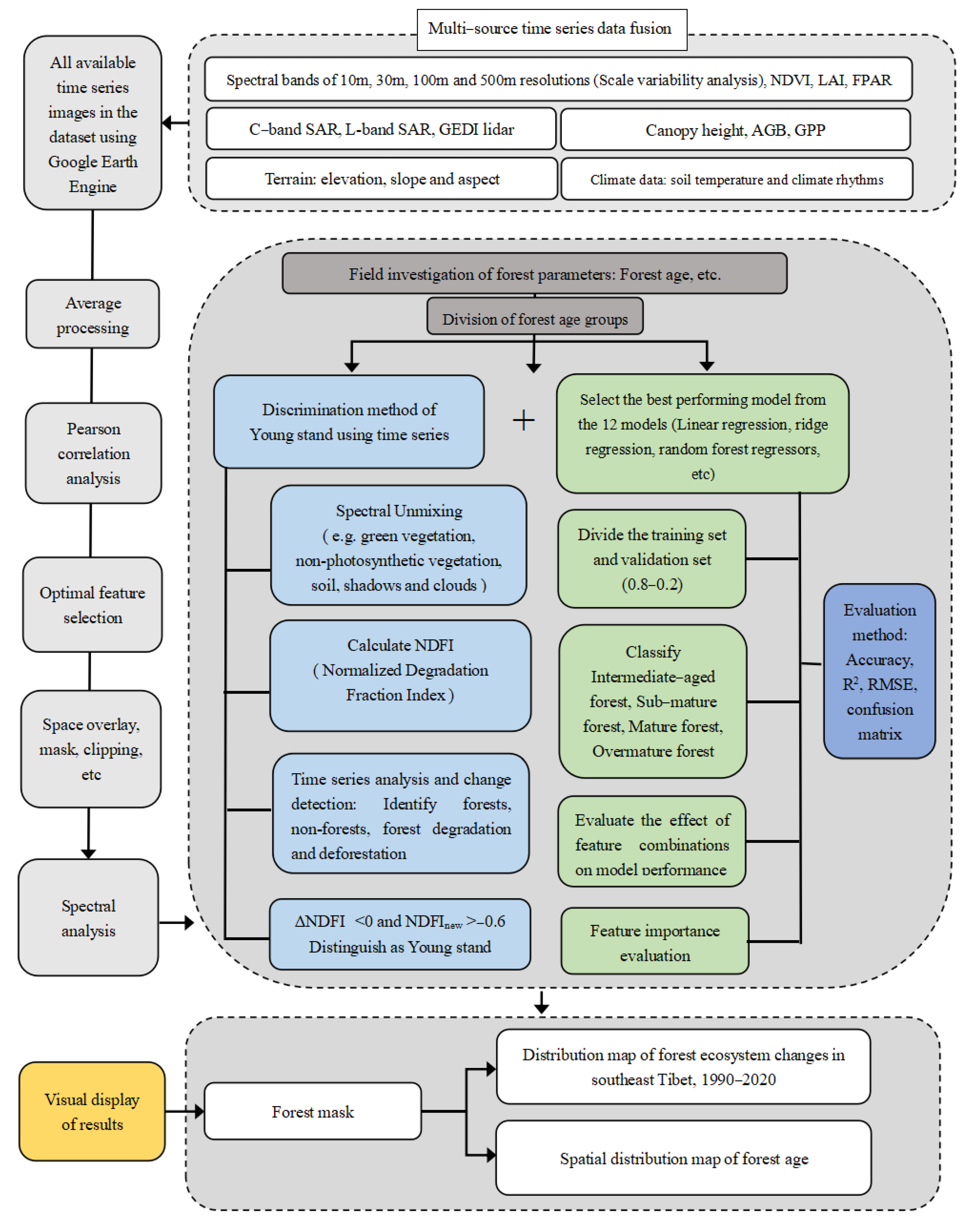
2.1. Research Strategy

This study systematically analyzed the spatial and temporal characteristics of forest ecosystems in Southeastern Tibet between 1990 and 2020 using a combination of multi-source remote-sensing data and machine-learning techniques (Figure 1). The study accurately identified forest degradation and deforestation and constructed age-distribution maps of forests. To identify the distribution of forest age groups, we employed the Continuous Degradation Detection (CODED) algorithm combined with Normalized Difference Fraction Index (NDFI) time-series data from 1990 to 2020 to detect young forests. For other age groups, we used machine-learning algorithms with multi-source remote-sensing data from 2020. Training samples were constructed over extended time intervals (e.g., 40 years for mature forests) to account for potential spectral changes over time and to improve the robustness of the model. This approach leverages the stability of spectral characteristics within each age group over longer periods, enhancing the model’s ability to generalize across temporal variations.

• Data Collection

A rich and diverse dataset was accessed from the GEE platform, including spectral bands of different resolutions (to identify scale variability in the spectral patterns of forest age), C-band synthetic aperture radar (C-band SAR), L-band synthetic aperture radar (L-band SAR), and Global Ecosystem Dynamics Investigation (GEDI) LiDAR data. Additionally, topographic data (e.g., elevation, slope, aspect), climate variables, and vegetation products (e.g., canopy height, biomass, productivity, NDVI, LAI, FPAR) were integrated. These data cover all available time spans in the GEE dataset, ensuring comprehensive spatiotemporal information to capture forest ecosystem dynamics. Scale analyses were conducted at four spatial resolutions (10, 30, 100, and 500 m) to explore the spectral patterns of forest age and identify the appropriate scale for the study. Pearson correlation analysis was used to explore the relationships between forest age and key variables, including passive remote-sensing products, terrain, and climate factors.

• Data Fusion and Preprocessing

To ensure data consistency and integrity, data fusion and preprocessing were implemented. This included calculating variable means to reduce noise, identifying key features using Pearson correlation analysis, and selecting the most predictive variables for the model. The estimability of different feature combinations (e.g., optical, SAR, LiDAR) was evaluated. Spatial processing operations, such as overlay, masking, and clipping, were also performed to prepare the data for subsequent analysis.

• Field Surveys and Target Analysis

Field surveys focused on key forest parameters, particularly forest age. Forests were classified into five age groups: young, intermediate-aged, sub-mature, mature, and overmature. Young stand forests were identified using time-series methods, while other age groups were classified using machine-learning techniques.

• Model Selection and Evaluation

The performance of 12 regression models (e.g., linear regression, ridge regression, random forest regression) was assessed to select the best model for describing forest ecosystem changes. This process not only improved model accuracy but also provided reliable methodological support for subsequent analysis.

• Detailed Classification Using the CODED Algorithm

The CODED algorithm, spectral decomposition, normalized difference fraction index (NDFI) calculations [50], and time series analysis were employed to classify forest cover changes from 1990 to 2020, thereby clarifying the spatial distribution of young forests.

• Feature Combination and Model Performance Analysis

The impact of different feature combinations on model performance was analyzed to optimize the model structure and improve prediction accuracy.

• Results Visualization and Systematic Evaluation

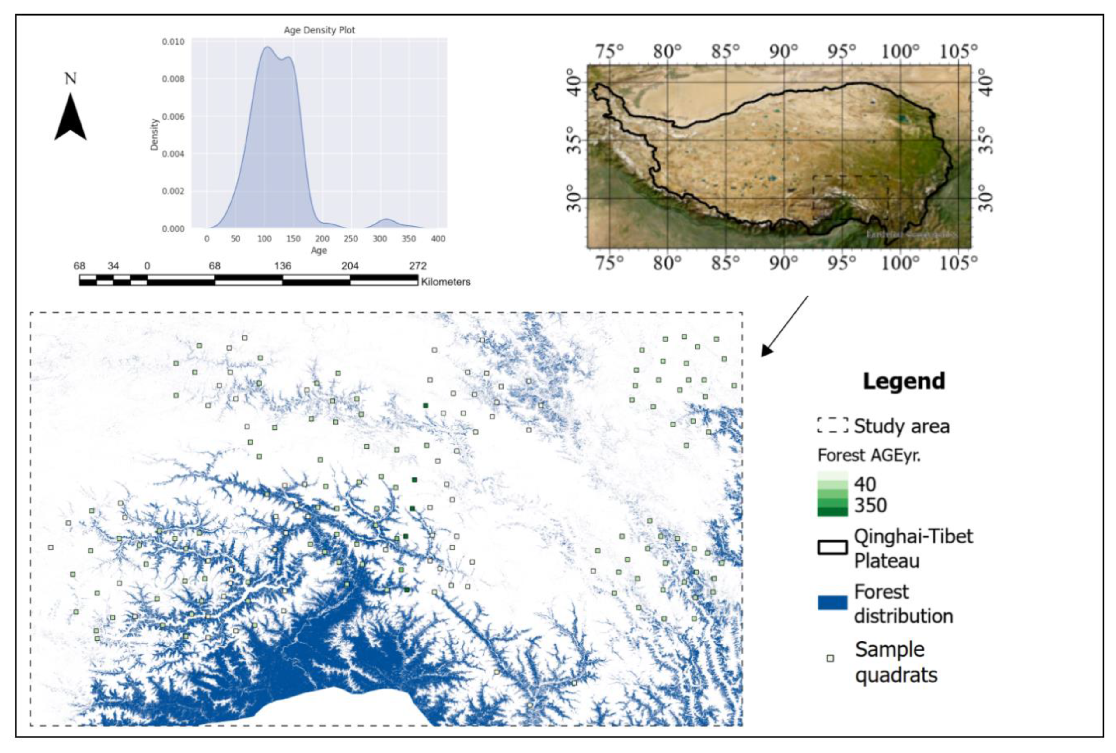
The results were visualized through maps of forest ecosystem changes and spatial distributions of forest age. Systematic evaluation was conducted using metrics such as confusion matrices, accuracy, coefficient of determination (R²), and root mean square error (RMSE).

2.2. Research Area

The study area, situated on the southeastern margin of the Tibetan Plateau (Figure 2), spans from 28.2267°N to 31.9495°N and from 92.4905°E to 98.9131°E, covering an area of approximately 294,000 km². Referred to as the “roof of the world”, the Qinghai–Tibet Plateau has an average elevation exceeding 4000 m and exhibits distinctive topographic and surface features [51], making it a critical region for studying complex climate and vegetation dynamics [52,53,54]. The vegetation cover in this area is both complex and systematic, transitioning gradually from forests in the southeast to deserts in the northwest, encompassing a wide variety of vegetation types [55,56].

Southeastern Tibet is predominantly covered by pristine forests and lies in the transition zone between the Assam Plain of India and the Tibetan Plateau [57]. The region’s steep mountain valleys, ranging in altitude from 143 to 7728 m, were shaped by the Miocene Yanshan movement and Quaternary crustal uplift, creating distinct vertical zonation [58]. Heavily influenced by the Indian Ocean monsoon, this area hosts China’s largest pristine forest and exhibits significant vertical differentiation in climate and vegetation, representing most vegetation and climate types found in the Northern Hemisphere. It serves as an ideal location for alpine ecosystem research, featuring the world’s highest forest line and a crisscrossing forest zone with strong microhabitat variations, high environmental heterogeneity, and rich biodiversity [59].

Located at the eastern terminus of the Himalayas, Southeastern Tibet is recognized as one of the world’s biodiversity hotspots and one of 200 globally important ecological regions. Land-cover changes are complex due to variations in altitude and climate. As a primary channel for water vapor transport from the Indian Ocean monsoon, the region is characterized by abundant cloud cover, making remote-sensing studies challenging [18,48]. Additionally, limited accessibility and scarce field samples have resulted in few studies conducted in this area. This study addresses key challenges in forest age remote-sensing research in cloudy mountainous regions, including cloud contamination, limited validation points, and complex, fragmented terrain. Based on the distribution of field sample data, the central box area in Figure 2 was identified as the focal research area.

2.3. Field Data and Forest Age Groups

The study area exhibits a complete series of altitudinal vegetation types, ranging from alpine snow and ice belts to low-valley tropical monsoon rainforests, demonstrating a broad and complex altitudinal vegetation gradient. The dark coniferous forests include species such as Abies georgei var. smithii, and Picea linzhiensis, while the bright coniferous forests feature Pinus yunnanensis and Pinus densata [60]. Most of these forests remain pristine and undisturbed.

For this study, we employed a field inventory dataset completed in 2010 by the forestry sector. This database integrates historical survey data from forestry departments and institutions such as the Chinese Academy of Sciences, as well as standard-sample forest inventory data. It encompasses key parameters, including forest age, tree density, biomass, and productivity. Forest age was calculated as the average age of dominant trees within 1-hectare sample plots. After validation, data from 200 sample plots (each 1 hectare in size) were used for analysis (see

Table A1. Table of parameters for field forest surveys.

Classification of Forest Parameters	Parameter Name	Describe
Age	AGEyr.	Forest age (years) is the average age of the dominant tree species.
Leaf area	TREE-LAI	Tree leaf-area index
Volume	VOLUMEm3/ha	Volume of wood per hectare
Tree Density	DENSITYtrees/ha	Density of trees per hectare
Biomass	STEM_MASSt.DM/ha	Biomass per hectare of tree trunk (dry matter)
	BRANCH_MASSt./ha	Biological number of branches per hectare
	LEAF_MASSt./ha	Leaf biomass per hectare
	ROOT_MASSt.DM/ha	Root biomass (dry matter) per hectare
	TOTAL_TREE_MASSt.DM/ha	Total tree biomass per hectare
	HERB-MASSt.DM/ha	Herbaceous biomass per hectare
	SHRUB-MASSt./ha	Shrub biomass per hectare
	TOTAL-MASSt.DM/ha	Total biomass per hectare (trees, shrubs, herbs)
Primary productivity	STEM_NPPt.DM/ha/yr.	Primary productivity per hectare of tree trunk (dry matter)
	BRANCH_NPPt.DM/ha/yr.	Primary productivity per hectare of branches
	LEAF_NPPt.DM/ha/yr.	Primary productivity per hectare of leaves
	ROOT_NPPt.DM/ha/yr.	Primary productivity per hectare of roots
	TOTAL_TREE_NPPt.DM/ha/yr.	Total tree primary productivity per hectare
	HERB-NPPt./ha/yr.	Primary productivity per hectare of herbs
	SHRUB-NPPt.DM/ha/yr.	Primary productivity per hectare of shrub
	TOTAL-NPPt.DM/ha/yr.	Total primary productivity per hectare
Geographic information	Altitude	Altitude
	LATITUDE,deg.	North latitude
	LONGITUDEE,deg.	East longitude

for specific parameters).

Figure 2 (Age Density Plot) reveals that the forest age distribution exhibits a prominent single peak around 100 years, indicating a high concentration of trees approximately 100 years old in the study area. The age distribution is primarily concentrated between 0 and 200 years, with a smaller secondary peak around 300 years, suggesting the presence of a small number of long-lived trees. Overall, the age distribution is relatively concentrated, with the majority of trees being less than 200 years old and relatively few exceeding this age.

Based on the Chinese forestry industry standard, “Regulations for age-class and age-group division of main tree species [61]”, forest ages were divided into five subgroups (

Table 1. Forest age group table.

Age Groups	Age Range	Description
Young forest	<40 years	Trees in early growth stage with underdeveloped canopies and unstable stand structure.
Intermediate-aged forest	40–60 years	Vigorously growing trees forming closed canopies with rapid height and diameter increases.
Sub-mature forest	60–80 years	Trees approaching physiological maturity with slowing growth but accumulating economic value.
Mature forest	80–120 years	Trees at peak utilization stage with optimal timber quality and ecological functions.
Overmature forest	>120 years	Declining trees with stagnant growth, increased vulnerability to pests and diseases.

): young forest (<40 years), intermediate-aged forest (40–60 years), sub-mature forest (60–80 years), mature forest (80–120 years), and overmature forest (>120 years). Notably, no samples of young forest (<40 years) were available in the study area, so this group was excluded from the analysis. The age-distribution sample size of the forest shown in Figure 3 varies depending on the maturity of the forest, with 7 intermediate-aged forests, 20 sub-mature forests, and 83 mature forests. For mature forests, the sample size is relatively large. This is because overripe forests have a wider distribution range in the study area, and for some young forest types, the sample size may be relatively small. These data are indeed consistent with the fact that Southeastern Tibet is a primitive forest.

The violin plot in Figure 3 illustrates the distribution of forest age data across the four forest age groups. The violin diagram shows the distribution of forest age data for four different forest age groups. The forest age distribution in intermediate-aged and sub-mature forests is concentrated, with a narrow density curve, indicating high forest age consistency. The wide and multi-peaked distribution of mature forests indicates multiple age levels. The distribution of overmature forests is particularly wide, especially in high-age areas, indicating significant variability in forest age. Intermediate-aged and sub-mature forests have low medians and small quartile spacings, indicating a concentrated distribution. Mature forests show high medians and large quartile differences, with a wide distribution. There are discrete points in the intermediate-aged and sub-mature forests. There are no obvious outliers in mature and overmature forests, but the broad distribution of overmature trees may include extreme values. As forests age, the variability in forest age distribution increases. Two key characteristics emerge from the data distribution: 1. As forests progress to more mature stages, the variability in forest age distribution increases. 2. Extreme values in the older age group (representing particularly old trees) are significant data points rather than noise in forest age remote-sensing studies. However, the sample size of older trees in this study was limited (only seven samples over 200 years old).

2.4. Multi-Source Time-Series Remote-Sensing Data Fusion

To further improve the accuracy of the regression and integrate a large amount of relevant information, this study uses the powerful computing power and abundant data resources of the GEE platform to conduct a comprehensive assessment of forest age. The GEE platform’s mean function (ee.ImageCollection.mean () method) consolidates all available long time-series data into a single mean image. This not only effectively reduces the data volume and retains more complete spatial and temporal information on critical long-sequence forest ecosystems, but it also reduces cloud pollution interference to facilitate subsequent analytical work [62]. In the present study, all remote-sensing datasets with time-series data are processed using a mean function method, with the aim of fully exploiting the rich information contained in these datasets. The time span of the selected dataset is all available time periods in the GEE platform. This study is aimed at applying a comprehensive approach of multiple angles and multiple sensors to improve the accuracy of forest age estimation. The dataset involved covers a wide range of information, including passive remote sensing, active remote sensing, and structural parameters of forest ecosystems, and it covers different scales (detailed list in

Table A2. Table of multi-source remote-sensing data.

Data Set	Abbreviated Name	Describe	Dataset Id (GEE)
ETH Global Sentinel-2 10 m Canopy Height (2020)	CAPHEI	Fusing GEDI with Sentinel-2 to generate probabilistic deep learning models for global retrieval of canopy height [83].	users/nlang/ETH_GlobalCanopyHeight_2020_10m_v1
Sensor-Independent MODIS and VIIRS LAI/FPAR CDR 2000 to 2022 (8d500m)	LAI	Leaf-Area Index (LAI), used to characterize the state of terrestrial ecosystems [84].	projects/sat-io/open-datasets/BU_LAI_FPAR/wgs_500m_8d
Sensor-Independent MODIS & VIIRS LAI/FPAR CDR 2000 to 2022 (8d500m)	FPAR	Fraction of Photosynthetically Active Radiation (FPAR), used to characterize terrestrial ecosystem states.	projects/sat-io/open-datasets/BU_LAI_FPAR/wgs_500m_8d
Global Aboveground and Belowground Biomass Carbon Density Maps at 300 m Resolution (2010)	AGB	Living biomass carbon reserve density on wood and grassy vegetation in 2010. This includes the carbon stored in the living plant tissue (stems, bark, branches, twigs) located above the surface. This does not include fallen leaves or rough woody fragments that once attached to living plants but were later deposited and are no longer viable [85].	NASA/ORNL/biomass_carbon_density/v1
MOD17A3HGF.061: Terra Net Primary Production Gap-Filled Yearly Global 500 m (2001–2023)	GPP	Gross primary productivity [86].	MODIS/061/MOD17A3HGF
SBIO1_Annual_Mean_Temperature (1000 m)	AMT	Average annual temperature, which indicates the average temperature at soil depth of 0–5 cm during the year (ecosystem conditions below the vegetation crown and near the surface) [87].	projects/crowtherlab/soil_bioclim/SBIO_v2_0_5cm
SBIO2_Mean_Diurnal_Range (1000 m)	MDR	Mean daily range of temperature, i.e., –5 cm of soil depth. The average difference between the highest and lowest temperatures on a day.	projects/crowtherlab/soil_bioclim/SBIO_v2_0_5cm
SBIO3_Isothermality (1000 m)	S_I	The isotherm of soil depth of 0–5 cm, the formula is BIO2/BIO7 × 100, which reflects the uniformity of temperature change.	projects/crowtherlab/soil_bioclim/SBIO_v2_0_5cm
SBIO4_Temperature_Seasonality (1000 m)	STS	The seasonal temperature change of 0–5 cm soil depth, measured as a standard deviation, indicates the dispersion of temperature changes over a year.	projects/crowtherlab/soil_bioclim/SBIO_v2_0_5cm
SBIO5_Max_Temperature_of_Warmest_Month (1000 m)	SMTWM	The hottest monthly maximum temperature of 0–5 cm of soil depth indicates the maximum temperature in the hottest month of the year.	projects/crowtherlab/soil_bioclim/SBIO_v2_0_5cm
SBIO6_Min_Temperature_of_Coldest_Month (1000 m)	SMTCM	The coldest monthly minimum temperature of 0–5 cm of soil depth indicates the lowest temperature in the coldest month of the year.	projects/crowtherlab/soil_bioclim/SBIO_v2_0_5cm
SBIO7_Temperature_Annual_Range (1000 m)	TARa	The annual temperature range of 0–5 cm soil depth, the formula BIO5-BIO6, that is, the difference between the highest temperature of the hottest month and the lowest temperature of the coldest month.	projects/crowtherlab/soil_bioclim/SBIO_v2_0_5cm
SBIO8_Mean_Temperature_of_Wettest_Quarter (1000 m)	MTWQ	The wettest quarterly mean temperature of 0–5 cm of soil depth indicates the average temperature of the wettest quarter of the year.	projects/crowtherlab/soil_bioclim/SBIO_v2_0_5cm
SBIO9_Mean_Temperature_of_Driest_Quarter (1000 m)	MTDQ	The driest quarterly mean temperature of 0–5 cm of soil depth indicates the average temperature of the driest quarter of the year.	projects/crowtherlab/soil_bioclim/SBIO_v2_0_5cm
SBIO10_Mean_Temperature_of_Warmest_Quarter (1000 m)	MTWQ_1	The warmest quarterly mean temperature of 0–5 cm of soil depth indicates the average temperature of the warmest quarter of the year.	projects/crowtherlab/soil_bioclim/SBIO_v2_0_5cm
SBIO11_Mean_Temperature_of_Coldest_Quarter (1000 m)	MTCQ	The coldest quarterly mean temperature of 0–5 cm of soil depth indicates the average temperature of the coldest quarter of the year.	projects/crowtherlab/soil_bioclim/SBIO_v2_0_5cm
Sentinel-1 SAR GRD: C-band Synthetic Aperture Radar Ground Range Detected, log scaling (2015–2023)	VV	Single-covalent polarization, vertical emission/vertical reception	COPERNICUS/S1_GRD
Sentinel-1 SAR GRD: C-band Synthetic Aperture Radar Ground Range Detected, log scaling (2015–2023)	VH	Two-band cross polarization, vertical emission/horizontal reception	COPERNICUS/S1_GRD
Global PALSAR-2/PALSAR Yearly Mosaic, version 1	HHLSAR	HH polarization backscattering coefficient, 16-bit DN [88].	JAXA/ALOS/PALSAR/YEARLY/SAR
Global PALSAR-2/PALSAR Yearly Mosaic, version 1	HVLSAR	HV polarization backscattering coefficient, 16-bit DN.	JAXA/ALOS/PALSAR/YEARLY/SAR
Gridded GEDI Vegetation Structure Metrics and Biomass Density, 1 km pixel size (2019–2023)	MEAN	The mean of GEDI shot metric values within a pixel [89].	LARSE/GEDI/GRIDDEDVEG_002/V1/1KM
Gridded GEDI Vegetation Structure Metrics and Biomass Density, 1 km pixel size (2019–2023)	MEANBASE	Standard error of the mean calculated using bootstrap resampling.	LARSE/GEDI/GRIDDEDVEG_002/V1/1KM
Gridded GEDI Vegetation Structure Metrics and Biomass Density, 1 km pixel size (2019–2023)	MEDIAN	The median value (50th percentile) of GEDI shot metric values within a pixel.	LARSE/GEDI/GRIDDEDVEG_002/V1/1KM
Gridded GEDI Vegetation Structure Metrics and Biomass Density, 1 km pixel size (2019–2023)	SD	The standard deviation of GEDI shot metric values within a pixel.	LARSE/GEDI/GRIDDEDVEG_002/V1/1KM
Gridded GEDI Vegetation Structure Metrics and Biomass Density, 1 km pixel size (2019–2023)	IQR	The interquartile range (75th percentile minus 25th percentile) of GEDI shot metric values within a pixel.	LARSE/GEDI/GRIDDEDVEG_002/V1/1KM
Gridded GEDI Vegetation Structure Metrics and Biomass Density, 1 km pixel size (2019–2023)	P95	The 95th percentile value of GEDI shot-metric values within a pixel.	LARSE/GEDI/GRIDDEDVEG_002/V1/1KM
Gridded GEDI Vegetation Structure Metrics and Biomass Density, 1 km pixel size (2019–2023)	Mountain	Shannon’s diversity index (H) of GEDI shot metric values within a pixel. Calculated as:-1(sum(plog(p))) where p is the proportion of GEDI shot values per bin.	LARSE/GEDI/GRIDDEDVEG_002/V1/1KM
Gridded GEDI Vegetation Structure Metrics and Biomass Density, 1 km pixel size (2019–2023)	COUNTF	The count of GEDI shot metric values within a pixel.	LARSE/GEDI/GRIDDEDVEG_002/V1/1KM
PROBA-V C1 Top Of Canopy Daily Synthesis 100 m (2013-)	RED	Top of canopy reflectance RED channel	VITO/PROBAV/C1/S1_TOC_100M
PROBA-V C1 Top Of Canopy Daily Synthesis 100 m (2013-)	NIR	Top of canopy reflectance NIR channel	VITO/PROBAV/C1/S1_TOC_100M
PROBA-V C1 Top Of Canopy Daily Synthesis 100 m (2013-)	BLUE	Top of canopy reflectance BLUE channel	VITO/PROBAV/C1/S1_TOC_100M
PROBA-V C1 Top Of Canopy Daily Synthesis 100 m (2013-)	SWIR	Top of canopy reflectance SWIR channel	VITO/PROBAV/C1/S1_TOC_100M
PROBA-V C1 Top Of Canopy Daily Synthesis 100 m (2013-)	NDVI	Normalized Difference Vegetation Index	VITO/PROBAV/C1/S1_TOC_100M
Harmonized Sentinel-2 MSI: MultiSpectral Instrument, Level-2A (2017–2024)		“B1”, “B2”, “B3”, “B4”, “B5”, “B6”, “B7”, “B8”, “B8A”, “B9”, “B11”, “B12”	COPERNICUS/S2_SR_HARMONIZED
Landsat Collection 2 (1990–2020)		“blue”, “green”, “red”, “nir”, “swir1”, “swir2” [90]
MOD09A1.061 Terra Surface Reflectance 8-Day Global 500 m (2000–2024)		"sur_refl_b01", "sur_refl_b02", "sur_refl_b03", "sur_refl_b04", "sur_refl_b05", "sur_refl_b06", "sur _ refl _ b07" [91]	MODIS/061/MOD09A1
NASADEM: NASA 30 m Digital Elevation Model	ELEVATION	Altitude [92]	NASA/NASADEM_HGT/001
NASADEM: NASA NASADEM Digital Elevation 30 m	SLOPE	Slope	NASA/NASADEM_HGT/001
NASADEM: NASA NASADEM Digital Elevation 30 m	ASPECT	The slopes are sloped	NASA/NASADEM_HGT/001

), providing strong support for a comprehensive analysis of the age of forest ecosystems.

• Spectroscopy, vegetation indices, and ecological remote-sensing product data:

We used MODIS and VIIRSLAI/FPAR CDR datasets to obtain leaf-area index (LAI) and photosynthetically active radiation absorption ratio (FPAR), which are critical for understanding photosynthesis and productivity in forests.

Using the high temporal resolution and high-resolution spectral reflectance data (100 m, daily cadence) provided by the Project for On-Board Autonomy—Vegetation (PROBA-V) dataset, we were able to capture subtle changes in the forest canopy, which is particularly important for distinguishing forests at different age stages.

In addition, we selected four remote-sensing datasets with different spatial resolutions: Sentinel-2 MSI (10 m), Landsat series (30 m), PROBA-V (100 m), and MOD09A1.061 Terra surface reflectance (500 m) to study: 1. The scale variability of remote-sensing spectra in different age groups of trees; 2. analyze the common age-spectrum relationships at different scales. The purpose is to reduce errors caused by scale effects. These datasets, with their unique spatiotemporal attributes and spatial resolutions, provide us with rich spectral information, enabling us to monitor and analyze the dynamic changes in forest ecosystems. By extracting features from key spectral bands, we quantify the characteristics of trees in different age groups. By comparing databases with different resolutions, we can discover potentially lost information. This comprehensive analysis method allows us to fully evaluate the scale variability in different age groups of trees.

In addition, we also used certain existing ecological remote-sensing products to provide insights into forest age, such as gross primary productivity.

• LiDAR forest structure and biomass data

The ETH Global Sentinel-2 Canopy Height dataset provides us with global information on canopy height, which is indispensable for estimating forest age and biomass.

The GEDI Vegetation Structure Indicator further provides information on forest structure and aboveground biomass carbon stock density. It uses LiDAR technology to obtain three-dimensional information about the Earth’s surface, such as vegetation height and canopy structure. These data are essential for understanding the carbon storage and dynamics of forests.

• Climate and Soil Data

Using the Global Dataset of Soil Bioclimatic Variables, we were able to incorporate environmental variables such as soil temperature and climate rhythms, which have a significant impact on assessing forest-growing conditions and age changes.

• SAR Data

Different SAR bands have different application advantages in forest monitoring, and selecting appropriate radar bands can improve the accuracy of forest structural parameter estimation. The Sentinel-1 synthetic aperture radar (SAR) dataset provides C-band SAR data, which are crucial for penetrating forest canopies and obtaining forest structural information, especially under cloud cover and suboptimal lighting conditions (except for extreme rainfall, where the backscattering signal from leaves and branches is affected by their moisture content, as reported by Westman and Paris in 1987). For C-band and X-band data, backscattering mainly comes from the leaves, small branches, or canopy top scattering of vegetation surfaces, while shrubs or ground cover contribute less to backscattering; for L-band data, backscattering mainly comes from tree trunks and branches. The L-band frequency allows for biomass measurements deeper into the forest. Therefore, we use the HH and HV polarization data from the ALOS/PALSAR dataset to further enhance our ability to monitor changes in forest structure. The L-band, due to its sensitivity to a forest’s internal structure, has an advantage in biomass measurements, while the C-band is more widely used for surface structure monitoring. The combination of both provides a comprehensive understanding of a forest’s age.

• Topographic data:

The elevation, slope, and aspect information provided by NASA’s DEM dataset are critical to understanding the impact of topography on forest distribution and growth.

This study integrates multi-source datasets with varying spatial resolutions. GEE employs an image pyramid strategy to dynamically select appropriate pyramid levels based on the output scale. By default, GEE resamples data using the nearest-neighbor method and adopts the output request’s specified scale parameter (or the map display’s zoom level) as the final resolution. To ensure consistency, all analyses in this study were constrained to a uniform resolution of 300 m. To further investigate the age characteristics of forests and their relationships with multi-source remote-sensing data and environmental factors in the valuable field data region of Southeastern Tibet, correlation analysis was employed to identify potential patterns. We performed Pearson correlation analyses for all forest parameters, ecological factors, and predictive characteristics to explore the linear correlation between factors.

2.5. Forest Change Detection and Age Identification

Remote-sensing time-series monitoring holds significant advantages in identifying young forests. Forest degradation and deforestation events, as key driving factors of forest age changes, have a profound impact on the age structure [63,64]. Accurate monitoring of these change processes and effective differentiation are of crucial importance for forest age mapping [65]. To this end, based on the GEE platform, this study employs the simplified continuous degradation detection (CODED) algorithm [33,34,66,67] to systematically evaluate the forest age dynamics through a three-stage analysis framework: (1) change detection; (2) classification of interference types; (3) age inference based on the degeneration–recovery process. In terms of concept definition, forest degradation is characterized by the continuous decline of vegetation coverage and ecosystem functions without the transformation of land-cover types. Although its NDFI index has decreased, it remains above the set threshold. In contrast, deforestation refers to the complete disappearance of forests and their transformation into non-forest land types (such as farmland or pastures), marked by a sharp drop in the NDFI value below the critical level. In this study, the CODED algorithm was applied to systematically analyze the change process of the forest ecosystem in the study area from 1990 to 2020, providing a basis for accurately determining the age of the forest. To enhance the detection accuracy, the following quality-control measures were specifically established: introducing a multi-level verification process to eliminate short-term interference noise; adopting a conservative threshold strategy; establishing a persistence test mechanism for time series. These measures have effectively mitigated the risk of misjudgment caused by low-intensity interference and significantly bolstered the reliability of the change-detection results. The specific technical route is as follows:

• Change Detection

Change detection was executed via spectral unmixing, which dissects satellite imagery into fundamental components, namely green vegetation (GV), non-photosynthetic vegetation (NPV), soil, shade, and clouds. Subsequently, the Normalized Degradation Fraction Index (NDFI) was computed to gauge forest health. High NDFI values (around 1) denote intact forests, while low values (around -1) signify degradation or deforestation.

$$\mathrm{G}\mathrm{V}\mathrm{s}\mathrm{h}\mathrm{a}\mathrm{d}\mathrm{e}={\displaystyle \frac{\mathrm{G}\mathrm{V}}{100-\mathrm{S}\mathrm{h}\mathrm{a}\mathrm{d}\mathrm{e}}}$$

(1)

$$\mathrm{N}\mathrm{D}\mathrm{F}\mathrm{I}={\displaystyle \frac{\mathrm{G}\mathrm{V}\mathrm{s}\mathrm{h}\mathrm{a}\mathrm{d}\mathrm{e}-(\mathrm{N}\mathrm{P}\mathrm{V}+\mathrm{S}\mathrm{o}\mathrm{i}\mathrm{l})}{\mathrm{G}\mathrm{V}\mathrm{s}\mathrm{h}\mathrm{a}\mathrm{d}\mathrm{e}+\mathrm{N}\mathrm{P}\mathrm{V}+\mathrm{S}\mathrm{o}\mathrm{i}\mathrm{l}}}$$

(2)

GV: Green vegetation score.

NPV: Non-photosynthetic vegetation fraction.

Soil: Soil fraction.

Shade: Shadow score.

Where GVshade is the shade-normalized GV fraction.

A time-series analysis spanning from 1990 to 2020 was employed to differentiate genuine changes from seasonal fluctuations by juxtaposing predicted and observed NDFI values. Significant deviations, represented as normalized residuals surpassing predefined thresholds, flagged potential disturbance events.

• Classification of Disturbances

The classification of disturbances distinguished forest degradation from deforestation. Forest degradation was identified by a gradual decline in NDFI while forest cover was still maintained, whereas deforestation was characterized by abrupt NDFI drops followed by land-cover conversion (e.g., to cropland). The adoption of conservative thresholds and persistence tests minimized false positives, thereby ensuring the reliable detection of both types of disturbances.

• Age Inference

Age inference was based on the history of disturbances and recovery trends. Areas that experienced degradation (but not deforestation) were categorized as young forests, reflecting recent disturbances with partial vegetation loss. By scrutinizing the timing, magnitude, and duration of NDFI declines, as well as subsequent recovery trends, we were able to estimate forest age. This provided crucial insights into ecosystem management and carbon cycle modeling.

2.6. Model Selection and Evaluation

To predict forest age, we first assessed the performance of 12 regression models through numerical regression to identify the optimal model. Subsequently, we utilized the classification pattern of the optimal model to classify forest age groups. This strategy can gradually simplify the complex problem of forest age prediction while ensuring the accuracy and interpretability of the prediction, providing more practical results for forest management and ecological research. The 12 regression models included Linear Regression, Ridge Regression, Lasso Regression, ElasticNet Regression, Decision Tree Regression, Random Forest Regression, Gradient Boosting Regression, Extra Forests Regression, K-Nearest Neighbor Regression, Support Vector Regression, Multilayer Perceptron Regression, and AdaBoost Regressor (

Table A3. The model table for comparison in the research.

Model Name	Description
Linear regression	Linear regression [93] models the relationship between the dependent variable (forest age) and the independent variables using a linear equation.
Ridge regression	Predicts forest age by shrinking coefficients with L2 regularization [94], suitable for handling multicollinearity.
Lasso regression	Predicts forest age by selecting important features with L1 regularization [95], suitable for high-dimensional data.
ElasticNet Regression	Predicts forest age by combining L1 and L2 regularization [96], suitable for high-dimensional data with multicollinearity.
Decision Tree Regression	Predicts forest age by recursively splitting data based on a forest structure [97], suitable for nonlinear relationships.
Random Forest Regression	Predicts forest age by averaging results from multiple decision forests [98], suitable for high-dimensional data requiring high accuracy.
Gradient Boosting Regression	Predicts forest age by sequentially adding weak learners to optimize the loss function [99], suitable for complex nonlinear relationships.
Extra forests Regression	Predicts forest age using random thresholds for splitting data [100], with faster training speed.
K-Nearest Neighbor Regression	Predicts forest age by averaging the values of the K nearest neighbors [101], suitable for low-dimensional data.
Support vector regression	Predicts forest age using a hyperplane and kernel functions [102], suitable for high-dimensional data.
Multilayer Perceptron Regression	Predicts forest age by fitting complex relationships with a neural network [103], suitable for large-scale data.
AdaBoost Regressor	Predicts forest age by training multiple weak learners with adjusted sample weights [104], suitable for improving model performance.

). After identifying the optimal regression model (Random Forest), we used its classification model to classify forest age groups (AGE_GROUP). Specifically, the random forest classifier is used to classify the four age groups (intermediate-aged forest, sub-mature forest, mature forest, and overmature forest). We systematically evaluated the impact of different feature combinations on classifier performance. Through a series of experiments, we determined the optimal feature set for forest age group classification. Specifically, we compared feature combinations derived from single-source data (e.g., C-band radar, L-band radar, and optical data) and multi-source data (e.g., radar, optical, ecological, and terrain data). Each feature combination was used to train a Random Forest classifier, and we employed the grid-search method to identify the optimal hyperparameters for the Random Forest model. The model was built with 250 trees and implemented through the Google Earth Engine platform. The dataset was randomly divided into a training set (80%) and a validation set (20%). The classifier’s performance was ultimately evaluated by assessing its performance on the validation set. Additionally, we evaluated and analyzed the feature-importance scores of the best model to identify the key predictive factors for forest age. Ultimately, the results of random forest classification can be combined with the results of young forests using CODED to plot the age distribution of forests in Southeastern Tibet.

When evaluating the optimal model, we utilized Python 3.0 along with the machine-learning library scikit-learn, configured the default parameters, and employed 12 regression models to predict the age of the forest. The dataset used for regression was based on field-measured forest age data (sample size = 200), which was randomly divided into a training set (80%) and a testing set (20%) to evaluate the generalization ability of the models. Each model was trained using a set of predictor variables, such as CAPHEI, LAI, FPAR, agb_, AMT, MDR, S_I, STS, SMTWM, SMTCM, TARa, MTWQ, MTDQ, MTWQ_1, MTCQ, VV, VH, RED, NIR, BLUE, SWIR, NDVI, HHLSAR, HVLSAR, mean, meanbase, median, sd, iqr, p95, shan, countf, elevation, slope, and aspect (the meanings of these variables are provided in Table A2). We quantified model performance using RMSE and R² and selected the model with the best performance for forest age prediction.

2.7. Methods of Evaluation

To evaluate the accuracy of the proposed method in this study, we first used R² (coefficient of determination) and root mean square error (RMSE) to assess the regression performance of the regression model, and then used accuracy and confusion matrices to evaluate the accuracy of forest age group classification [68].

Accuracy: Refers to the ratio of the number of samples correctly predicted by the model to the total number of samples.

$$\mathrm{A}\mathrm{c}\mathrm{c}\mathrm{u}\mathrm{r}\mathrm{a}\mathrm{c}\mathrm{y}={\displaystyle \frac{\mathrm{T}\mathrm{P}+\mathrm{T}\mathrm{N}}{\mathrm{T}\mathrm{P}+\mathrm{T}\mathrm{N}+\mathrm{F}\mathrm{P}+\mathrm{F}\mathrm{N}}}$$

(3)

Among them:

TP (True Positives): True positives, which refer to the number of samples that are actually positive and predicted as positive.

TN (True Negatives): True negative, the number of samples that are actually negative and predicted as negative.

FP (False Positives): The number of samples that are actually negative but predicted as positive.

FN (False Negatives): The number of samples that are actually positive but predicted as negative.

The R² and RMSE were chosen to evaluate the goodness-of-fit of the regression model as follows:

$${\mathrm{R}}^2=1-{\displaystyle \frac{{\sum }_{\mathrm{i}=1}^{\mathrm{n}} ({\mathrm{y}}_{\mathrm{i}}-{\widehat{\mathrm{y}}}_{\mathrm{i}}{)}^2}{{\sum }_{\mathrm{i}=1}^{\mathrm{n}} ({\mathrm{y}}_{\mathrm{i}}-\overline{\mathrm{y}}{)}^2}}$$

(4)

$$\mathrm{R}\mathrm{M}\mathrm{S}\mathrm{E}=\sqrt{{\displaystyle \frac{1}{\mathrm{n}}}\sum _{\mathrm{i}=1}^{\mathrm{n}} {\left({\mathrm{y}}_{\mathrm{i}}-{\widehat{\mathrm{y}}}_{\mathrm{i}}\right)}^2}$$

(5)

where ${\mathrm{y}}_{\mathrm{i}}$ is the observed value, which ${\widehat{\mathrm{y}}}_{\mathrm{i}}$ is the model prediction, and n is the sample size.

3. Results

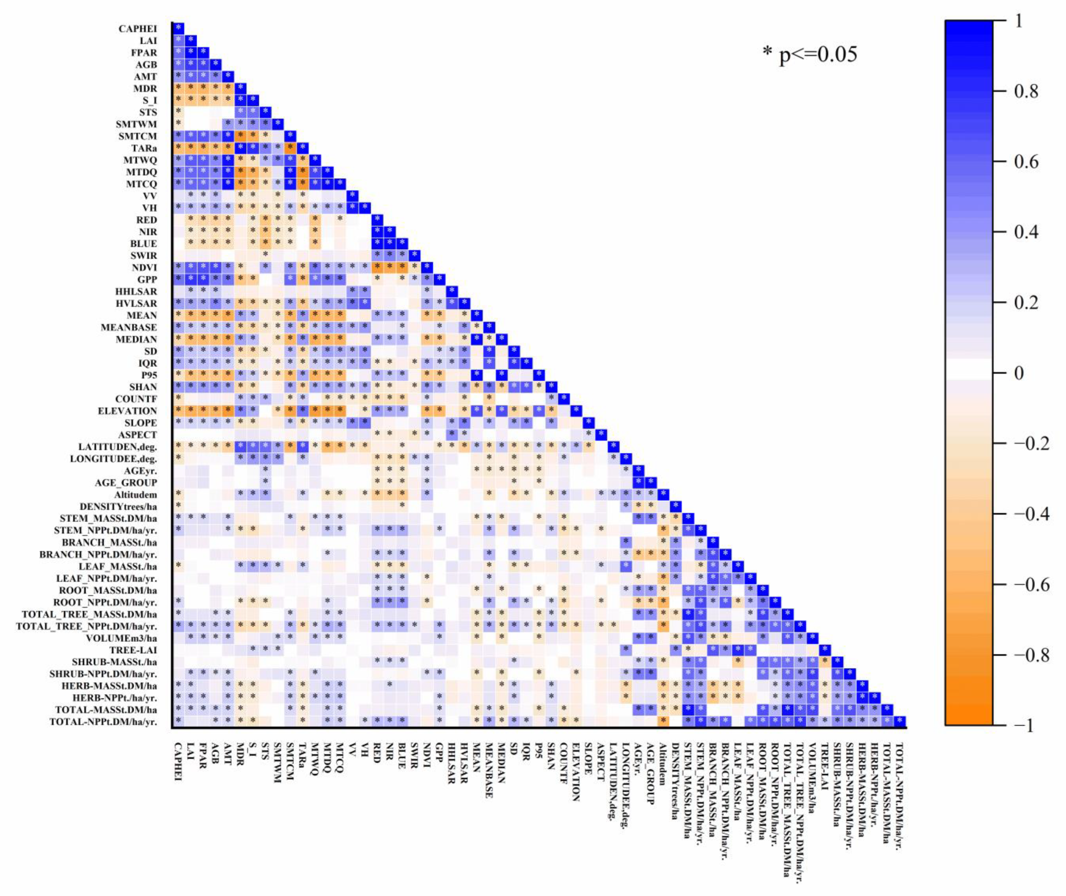
3.1. Correlation Analysis of Forest Age with Biomass and Ecological Variables

In this study, we analyzed the Pearson correlation between forest age (AGEyr) and multiple ecological and biomass-related variables using data from all field sampling points, with a significance level set at p < 0.05. The results showed a significant correlation between forest age and several variables (Figure 4). These variables include tree trunk biomass per hectare (STEM_MASSt.DM/ha), net primary productivity of branches (BRANCH_NPPt.DM/ha/yr.), root mass (ROOT_MASSt/ha), total tree mass (TOTAL_TREE_MASSt.DM/ha), volume (VOLUMEm³/ha), leaf-area index (TREE-LAI), shrub mass (SHRUB-MASSt/ha), average annual temperature (AMT), seasonal temperature change (STS), annual temperature range (TARa), near-infrared reflectivity (NIR), total primary productivity (GPP), HHLSAR, and HVLSAR.

Among the positively correlated variables, stem biomass (correlation coefficient = 0.54), leaf-area index (correlation coefficient = 0.53), volume (correlation coefficient = 0.49), and total tree mass (correlation coefficient = 0.48) showed moderate positive correlations (correlation coefficient between 0.40 and 0.69). These results indicate that the values of these variables tend to increase as trees age, reflecting the accumulation of biomass during growth. Additionally, the average annual temperature (correlation coefficient = 0.19), seasonal variation (correlation coefficient = 0.19), annual temperature range (correlation coefficient = 0.16), NIR reflectance (correlation coefficient = 0.15), and GPP (correlation coefficient = 0.19) showed weak positive correlations with forest age (correlation coefficient between 0.20 and 0.39). Although the relationship between these variables and forest age is not as strong as that of the variables listed above, it still shows some positive correlation.

Among the negatively correlated variables, branch net primary productivity (correlation coefficient = −0.44) showed a moderate negative correlation, indicating that the value of this variable tends to decrease with the age of the tree. Additionally, HHLSAR (correlation coefficient = −0.14) and HVLSAR (correlation coefficient = −0.18) showed weak negative correlations.

However, tree density (DENSITYtree/ha), stem net primary productivity (STEM_NPPt.DM/ha/yr.), branch mass (BRANC_MASSt/ha), leaf mass (LEAF_MASSt/ha), net primary productivity of leaves (LEAF_NPPt.DM/ha/yr.), net primary productivity of roots (ROOT_NPPt.DM/ha/yr.), total net primary productivity of trees (TOTAL_TREE_NPPst.DM/ha/yr.), net primary productivity of shrubs (SHRUB-NPPt.DM/ha/yr.), herb mass (HERB-MASSt.DM/ha), herb net primary productivity (HERB-NPPt.DM/ha/yr.), total net primary productivity (TOTAL-NPPt.DM/ha/yr.), canopy height (CAPHEI), leaf-area index (LAI), photosynthetically active radiation absorption ratio (FPAR), aboveground biomass carbon storage (AGB), mean-temperature diurnal range (MDR), isothermality (S_I), highest temperature in the hottest month (SMTWM), minimum temperature in the coldest month (SMTCM), mean temperature in the wettest quarter (MTWQ), mean temperature in the driest quarter (MTDQ), warmest quarterly mean temperature (MTWQ_1), coldest quarterly median temperature (MTCQ), vertically transmitted/vertically received radar echo (VV), red light reflectivity (RED), blue light reflectivity (BLUE), short-wave infrared reflectivity (SWIR), and the normalized vegetation index (NDVI) were not significantly correlated with forest age. These variables have a weak linear correlation with forest age.

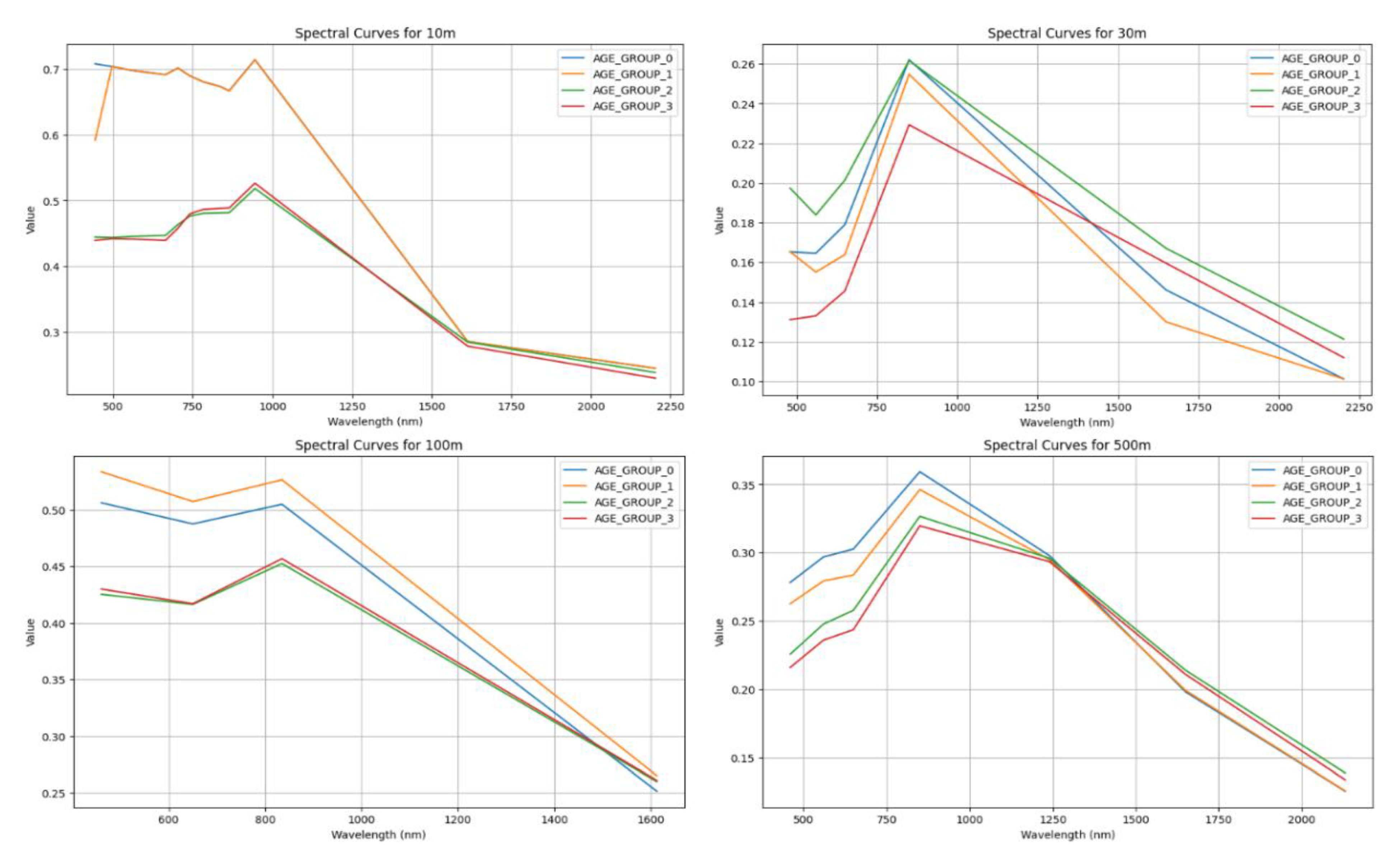
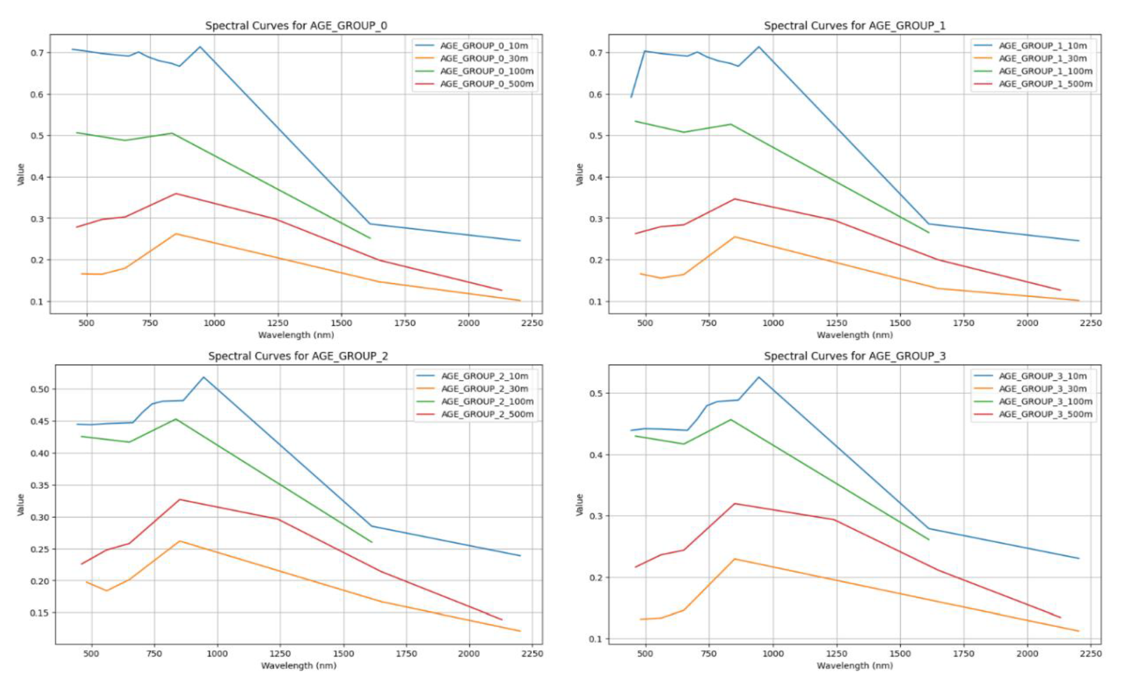
3.2. Forest Age Group—Scale Variability Relationship of Remote Sensing Spectroscopy

The spectral data we use come from different satellite sensors (such as 10 m of Sentinel-2 MSI, 30 m of Landsat series, 100 m of PROBA-V, and 500 m of MOD09A1), and the spatial resolutions of these sensors are different. The data from different sensors vary in spectral characteristics and spatial resolution. From Figure 5, it is evident that the spectral curves of different forest age groups exhibit distinct variations across various spatial resolutions while also sharing certain common characteristics. Specifically, significant differences in spectral reflectance are observed in specific wavelength ranges, which can be identified at different spatial resolutions. These variations provide a robust basis for distinguishing between forest age groups, further confirming the feasibility of utilizing remote-sensing spectral properties for forest age regression studies.

At a spatial resolution of 10 m, the spectral curves of each forest age group display a prominent peak near 1000 nanometers, followed by a gradual decline. Notably, the spectral curves of AGE_GROUP_0 and AGE_GROUP_1 are more similar, while those of AGE_GROUP_2 and AGE_GROUP_3 are lower and smoother, with significant differences in reflectance values between the former and latter groups.

At 30 m resolution, the spectral curves are relatively smooth overall, with less pronounced fluctuations compared to the 10 m resolution. When the spatial resolution is further reduced to 100 m, the spectral curves become even smoother. At this resolution, AGE_GROUP_0 and AGE_GROUP_1 maintain high reflectance values near 500 and 800 nanometers, whereas the curves of AGE_GROUP_2 and AGE_GROUP_3 are generally lower and decline rapidly beyond 850 nanometers.

At a resolution of 500 m, the peaks of the spectral curves are attenuated, and the overall reflectance levels stabilize. The curves of AGE_GROUP_0 and AGE_GROUP_1 retain high reflectance values near 800 nanometers, while those of AGE_GROUP_2 and AGE_GROUP_3 remain lower overall and exhibit a rapid decline beyond 800 nanometers.

In summary, as the spatial resolution decreases, the detailed information in the spectral curves gradually diminishes, the peaks weaken, and the curves become smoother. AGE_GROUP_0 and AGE_GROUP_1 exhibit higher spectral reflectance values in the shorter wavelength range (less than 1000 nanometers), whereas AGE_GROUP_2 and AGE_GROUP_3 show higher reflectance values in the longer wavelength range (greater than 1500 nanometers). Conversely, with increasing spatial resolution, the detailed characteristics of the spectral curves become more pronounced, and the differences between forest age groups are more distinct. High-resolution data capture finer details, enabling more precise analysis of the spectral characteristics of different forest age groups.

Based on the spatiotemporal resolution of the four remote-sensing products and the results of this study, we conclude that the 100 m spatial resolution product (PROBA-V C1 Top Of Canopy Daily Synthesis 100 m) is the most suitable for forest age prediction in this research. The spectral curves of the two age groups in the 100 m resolution data exhibited a high degree of similarity, with only minor variations observed. These curves were retained by the study for classification training purposes.

Figure 6 illustrates that spectral reflectance follows a consistent pattern across different forest age groups as wavelength changes. Specifically, the spectral reflectance of AGE_GROUP_0 generally decreases with increasing wavelength. Within the 500–1000 nanometer range, spectral curves exhibit significant variations at different spatial resolutions, with reflectivity differences being more pronounced at 10 m and 30 m resolutions.

For AGE_GROUP_1, spectral reflectance shows significant fluctuations in the 500–1000 nanometer range before gradually declining. Beyond 1000 nanometers, the curves exhibit more pronounced differences across resolutions. The spectral reflectance of AGE_GROUP_2 displays a distinct peak in the 500–1000 nanometer range, followed by a gradual decline, with notable variations in peak positions across resolutions. Similarly, AGE_GROUP_3 exhibits a peak in the 500–1000 nanometer range, after which reflectance gradually decreases.

At all spatial resolutions, the spectral curves of each forest age group show a declining trend in reflectance as wavelength increases. As forest age increases, spectral reflectance decreases in the short wavelength range (approximately 500–750 nanometers), while reflectance remains generally lower in the long wavelength range (1500–2250 nanometers). Additionally, spectral curves at different spatial resolutions exhibit significant differences in the short wavelength region, while reflectivity differences are relatively smaller in the long wavelength region.

Overall, the peak location and shape of spectral reflectance may vary with forest age, and spectral curves at different spatial resolutions show significant differences in specific wavelength ranges. These findings highlight the importance of spatial resolution and wavelength range in analyzing spectral reflectance patterns for distinguishing forest age groups.

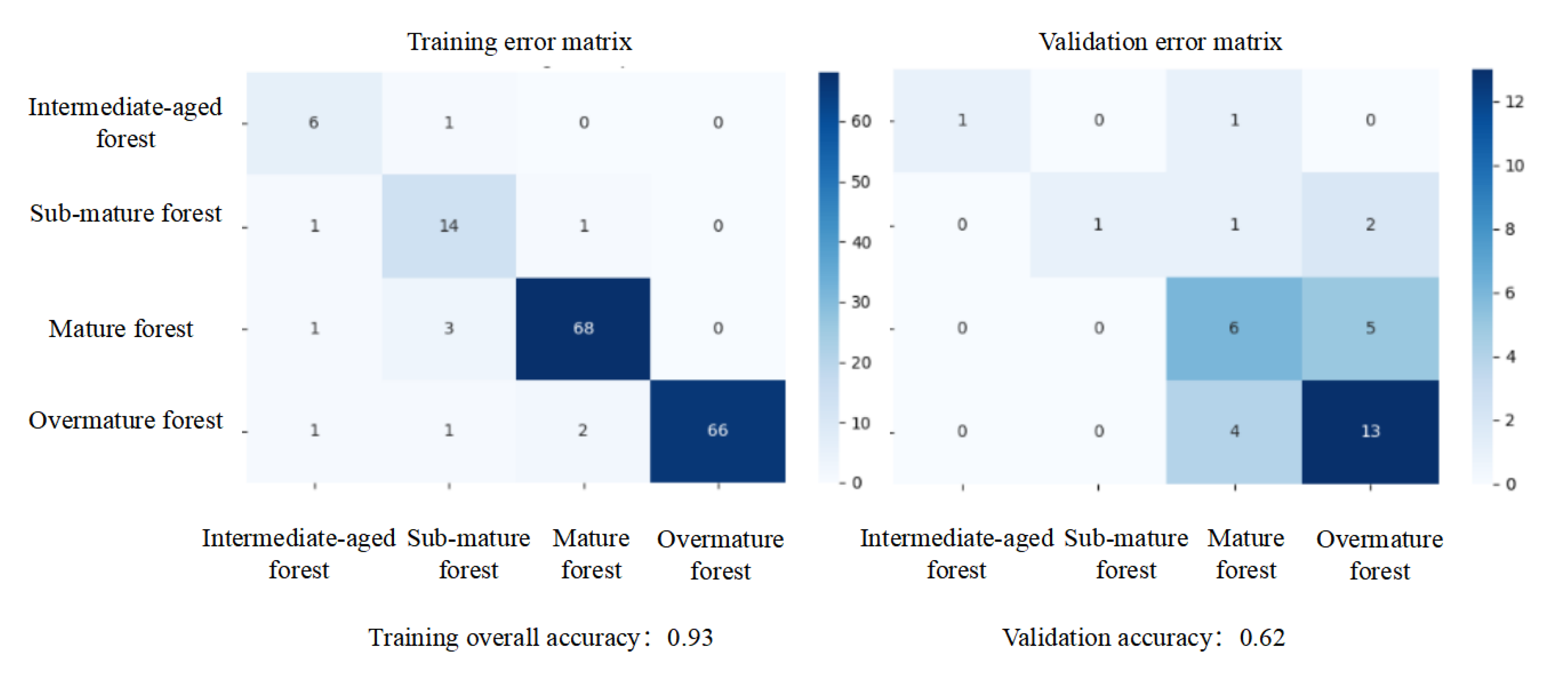
3.3. Model Performance

This study evaluated the performance of 12 regression models to identify the most suitable model for forest age prediction in Southeastern Tibet. Model performance was quantified using the RMSE and the R². The results are presented in

Table 2. Performance comparison between different models.

Model Name	RMSE	R2
Linear Regression	24.77	0.444
Ridge Regression	25.26	0.422
Lasso Regression	26.44	0.366
ElasticNet Regression	29.28	0.223
Decision Tree Regression	24.77	0.444
Random Forest Regression	25.39	0.466
Gradient Boosting Regression	24.77	0.444
Extra Forests Regression	24.77	0.444
K-Nearest Neighbor Regression	24.41	0.410
Support Vector Regression	34.13	−0.056
Multilayer Perceptron Regression	59.15	−2.171
AdaBoost Regressor	29.81	0.195

.

In the forest age-monitoring study conducted in Southeastern Tibet, Random Forest was identified as the optimal regression model based on a comprehensive evaluation of model performance and operational feasibility within the GEE platform. This model demonstrated superior predictive performance (RMSE = 25.39, R² = 0.466), significantly outperforming other approaches (e.g., support vector regression, which underperformed likely due to suboptimal default parameters). It is worth noting that linear regression achieves comparable accuracy. However, Random Forests offer additional advantages, including: (1) computational efficiency on GEE, (2) flexible parameter tuning, and (3) interpretable feature-importance analysis. These combined strengths position random forest as a robust technical solution for forest age mapping in topographically complex regions.

Other models that exhibited notable performance include Linear Regression (RMSE = 24.77, R² = 0.444) and Gradient-Boosting Regression (RMSE = 24.77, R² = 0.444). These models provided reasonable estimates of forest age, although their performance was slightly inferior to that of the Random Forest model.

Conversely, Support Vector Regression (SVR) and Multilayer Perceptron Regression (MLPRegressor) performed poorly, with R² values of −0.056 and −2.171, respectively. The negative R² values suggest that these models have limited predictive capacity for forest age estimation on the current dataset, potentially due to the complexity of the relationships between predictor variables and forest age.

Despite the potential advantages of Ridge Regression and Lasso Regression in mitigating multicollinearity among predictor variables, our results indicate that these methods underperformed compared to the Random Forest model. This finding suggests that ensemble methods, such as Random Forest, are more effective in balancing the reduction of multicollinearity and the enhancement of predictive accuracy. The Random Forest model’s ability to handle complex interactions among predictor variables and its robustness to overfitting make it particularly suitable for forest age estimation in this region.

In this study, we evaluated the effect of different combinations of features on the performance of random forest classifiers through a number of experiments. The following are the characteristic combinations and their corresponding classification accuracy manifestations (

Table 3. Comparing the performance of different feature combination models.

Feature Combination	Validation Accuracy
C-band radar band: VV, VH	0.45
L-band radar and GEDI feature combinations: HHLSAR, HVLSAR, mean, meanbase, median, sd, iqr, p95, shan, countf	0.42
Optical feature combinations: RED, NIR, BLUE, SWIR, NDVI	0.28
Radar and terrain feature combinations: VV, VH, HHLSAR, HVLSAR, mean, meanbase, median, sd, iqr, p95, shan, countf, elevation, slope, aspect	0.57
Ecological characteristics combination: CAPHEI, LAI, FPAR, Agb _, Gpp, AMT, MDR, S _ I, STS, SMTWM, SMTCM, TARa, MTWQ, MTDQ, MTWQ _ 1, MTCQ	0.55
Comprehensive combination of characteristics1 (Includes GEDI Data): CAPHEI, LAI, FPAR, agb_, AMT, MDR, S_I, STS, SMTWM, SMTCM, TARa, MTWQ, MTDQ, MTWQ_1, MTCQ, VV, VH, RED, NIR, BLUE, SWIR, NDVI, HHLSAR, HVLSAR, mean, meanbase, median, sd, iqr, p95, shan, countf, elevation, slope, aspect	0.65
Comprehensive combination of characteristics2 (Not including GEDI data)CAPHEI, LAI, FPAR, Agb_, AMT, MDR, S _ I, STS, SMTWM, SMTCM, TARa, MTWQ, MTDQ, MTWQ_1, MTCQ, VV, VH, RED, NIR, Blue, SWIR, NDVI, Gpp, HHLSAR,HVLSAR,elevation,slope,aspect	0.62

):

In this study, we compared the effects of different feature combinations on the performance of the random forest classifier. The classification accuracy of single data sources (e.g., C-band radar, L-band radar, and optical features) was relatively low, with validation accuracies of 0.45, 0.42, and 0.28, respectively. The combination of radar data and terrain features achieved a high classification accuracy (0.57). The ecosystem feature combination demonstrated high classification performance, achieving a validation accuracy of 0.55.

Furthermore, the classification accuracy of comprehensive feature combinations (including radar, optical, ecological, and topographic data) was notably enhanced. Composite Feature Set 1, which included GEDI LiDAR data, performed the best, with a validation accuracy of 0.65. In contrast, Composite Feature Set 2, which excluded GEDI LiDAR data, achieved a slightly lower validation accuracy of 0.62. These results indicate that multi-source data fusion, particularly when combined with LiDAR data, can significantly improve the accuracy of forest age group classification.

Therefore, this study demonstrates that integrating multi-source data, including radar, optical, ecological, and topographic features, is an effective strategy for enhancing forest age group classification accuracy. Considering the mesh coverage characteristics of GEDI data, we selected a comprehensive combination of characteristics and the random forest model for forest age prediction.

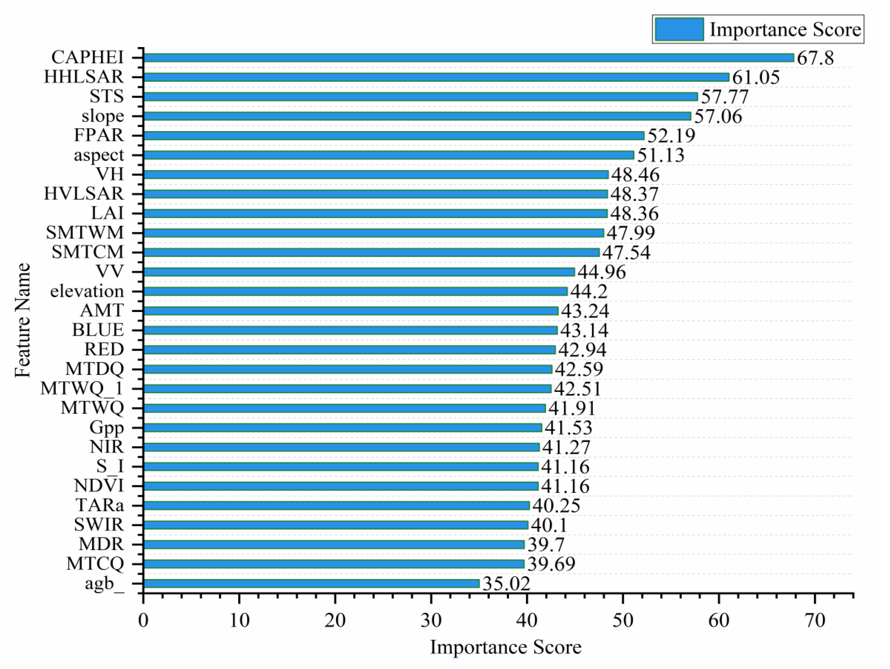
3.4. Evaluation of Forest Age Group Classification Results and Analysis of Characteristics of Predictors

Figure 7 demonstrates the performance of the model used for forest age group classification on both the training and validation sets, represented by two confusion matrices.

Training Set: The model performed exceptionally well, achieving an overall accuracy of 93%. Mature and overmature forests were classified with high precision, correctly identifying 68 and 66 samples, respectively.

Validation Set: The model’s overall accuracy dropped to 62%, indicating limited generalizability on unseen data. Specifically, significant classification confusion was observed between mature and overmature forests, with five and two samples misclassified, respectively. Additionally, there were errors in classifying intermediate-aged and sub-mature forests.

Figure 8 illustrates the feature-importance scores of the random forest model for forest age prediction. Among the features, CAPHEI (canopy height derived from LiDAR data) ranked highest with a score of 67.8, indicating its critical role in forest age prediction. This was followed by HHLSAR (horizontally transmitted and horizontally received synthetic aperture radar data) and STS (temperature seasonality), with scores of 61.05 and 57.77, respectively, highlighting their significant contributions to the model. Other important predictors included slope, photosynthetically active radiation absorption ratio (FPAR), and topographic aspect. In contrast, aboveground biomass (AGB) had the lowest importance score of 35.02, suggesting its limited contribution to forest age prediction.

These results emphasize the relative importance of LiDAR remote-sensing data, temperature seasonality, and topographic features in forest age assessment. They provide a scientific basis for optimizing predictive models for forest age.

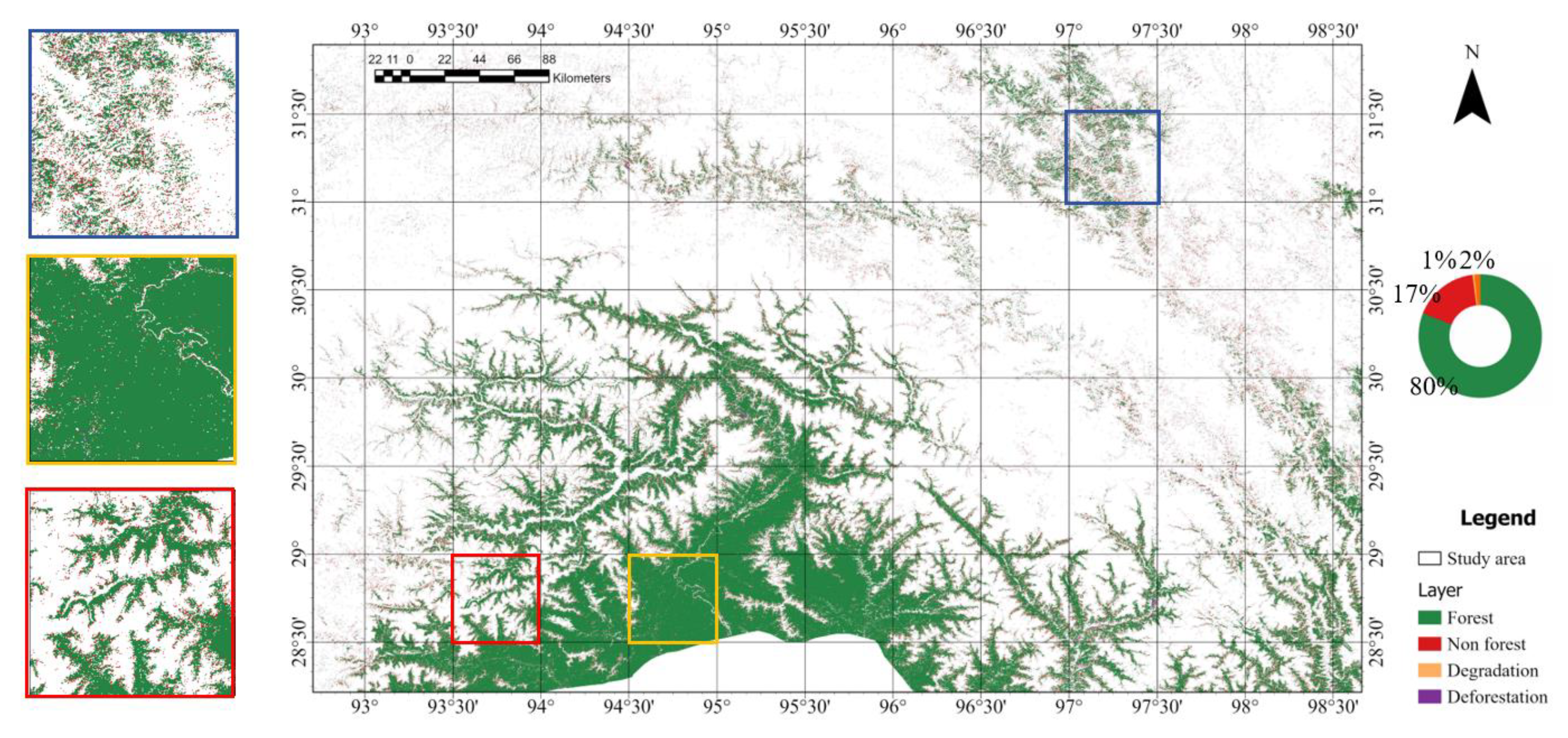
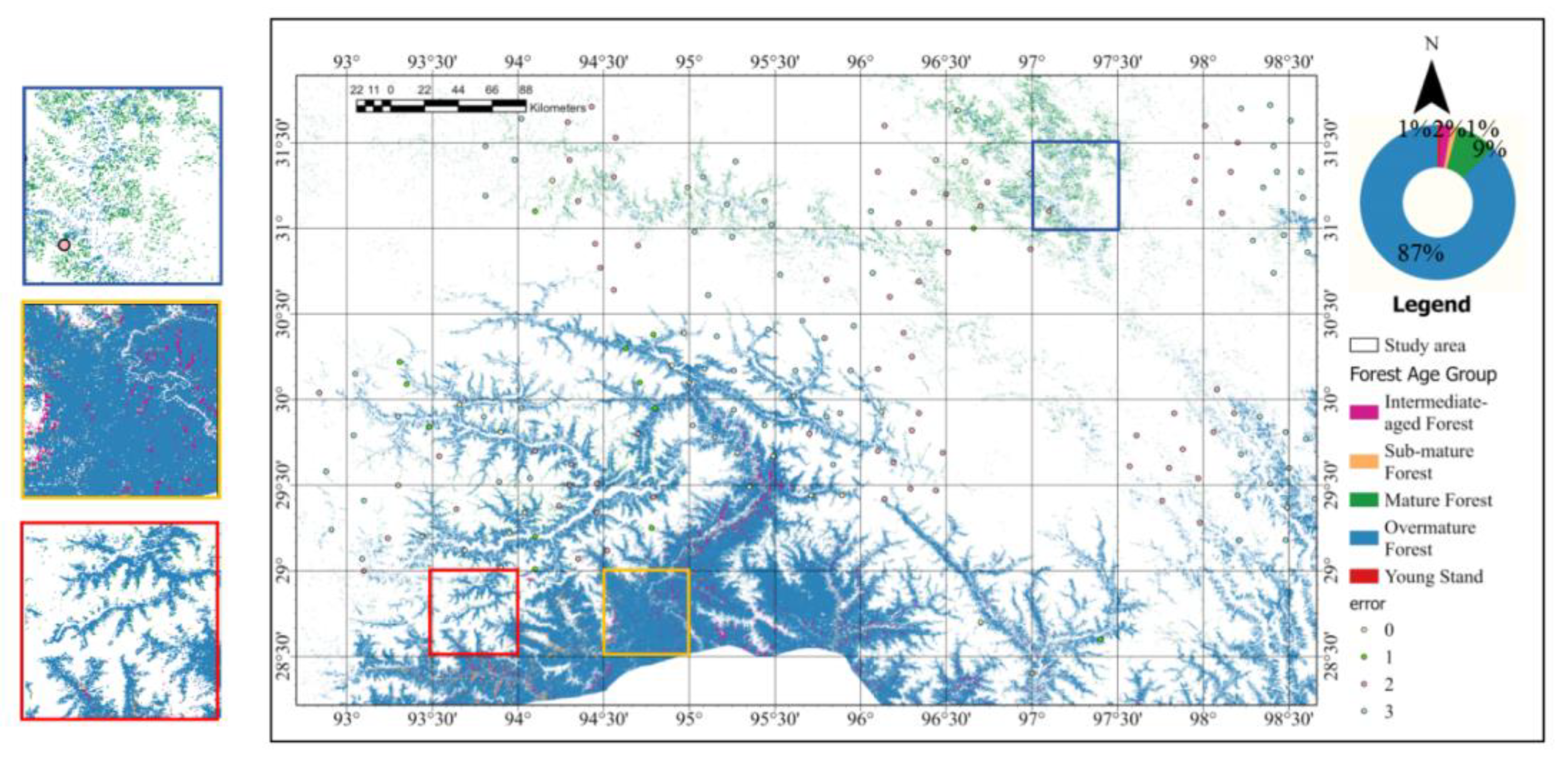
3.5. Spatial Distribution of Forest Age

In this study, the CODED algorithm was utilized to analyze time-series data of the Normalized Difference Fraction Index (NDFI), enabling the successful identification and classification of forest cover changes in Southeastern Tibet during the study period. Figure 9 provides a detailed distribution of forest cover changes between 1990 and 2020, including forested, non-forested, degraded, and deforested areas. Through spectral mixture analysis (SMA) and NDFI, this study achieved precise mapping and analysis of forest conditions in the region. Statistical results revealed that forested areas dominated the study region, accounting for 80% of the total area, while non-forested areas constituted 17%. Degraded and deforested areas represented 2% and 1%, respectively, indicating relatively low levels of deforestation and degradation despite some forest disturbances. On the map, green areas represent forested regions with NDFI values close to 1, reflecting their structural integrity and good health, while red areas denote non-forested regions with low NDFI values, indicating a lack of green vegetation cover. Degraded and deforested areas are marked in orange and purple, respectively, where NDFI values are significantly reduced due to vegetation loss and soil exposure. This study also conducted an in-depth analysis of the dynamic changes in Southeastern Tibet’s forest ecosystems between 1990 and 2020, including trends in deforestation, forest degradation, and the processes of forest restoration and regeneration. These findings are crucial for remote-sensing-based forest age identification in Southeastern Tibet, offering a deeper understanding of forest ecosystem dynamics and providing a scientific basis for forest age estimation.

Overmature forests dominate the forested areas in the study region, accounting for 87% of the total forest area (

Table 4. Research area statistics for the forest age group.

Forest Age Group	Total Area (m2)	Percentage of Total Area
Young forest	233,797,514.40	1%
Intermediate-aged forest	833,776,911.90	2%
Sub-mature forest	492,678,667.95	1%
Mature forest	3,275,570,584.65	9%
Overmature forest	33,472,546,497.30	87%
Total	38,308,370,176.20	100%

). This reflects the prevalence of mature and aging forests in the region (as shown in Figure 10). Mature forests represent 9% of the area, while intermediate-aged forests and young forests are significantly smaller, at 2% and 1%, respectively. The proportions of forest age groups depicted in the pie chart align with the color distribution on the map, where dark-blue areas, representing overmature forests, are the most prominent, further confirming the dominance of overmature trees (120-plus years of age) in the region. Further analysis revealed that geography significantly influences forest age distribution: younger forests are primarily found in river valleys, forest margins, and northern regions with relatively poor hydrothermal conditions, while older forests are concentrated in the south and within forest interior areas.

4. Discussion

4.1. Ecological Characteristics of Forest Age

This study reveals the ecological characteristics and spatial distribution patterns of forest age in Southeastern Tibet. It finds that overmature forests (over 120 years old) dominate the region [3], accounting for 87% of the forest area, while mature, intermediate-aged, and young forests constitute relatively smaller proportions. This predominantly mature forest age structure is likely influenced by the region’s natural environmental conditions [44], such as high altitude and low disturbance levels, as well as historical forest management practices [69].

In contrast, studies from other regions often report a higher proportion of mature and intermediate-aged forests and a lower proportion of overmature forests [7,23,26]. These differences may stem from variations in climatic conditions, forest types, human interference intensity, and historical fire events [31]. While the scarcity of field samples in southern forests may introduce some uncertainty, the detected widespread overmature forests are ecologically plausible, consistent with both model outputs and the documented status of Southeastern Tibet as China’s most extensive primary forest region [70]. The findings of this study underscore the diversity and complexity of forest age structures across different ecosystem contexts, emphasizing the need for region-specific forest management and conservation strategies.

4.2. The Influence of Forest Age on Spectral Reflectance Characteristics

Dynamic changes in leaf chlorophyll content and internal plant structure during the phenological cycle significantly influence spectral response patterns [71,72], with mature canopy leaves often exhibiting higher near-infrared and red light reflectance contrast characteristics [73]. This study revealed the significant effect of forest age on spectral reflectance by analyzing the spectral characteristics of different forest age groups. The results showed that spectral curves of different age groups exhibited notable differences in the short-wavelength (500–1000 nm) ranges. Young forests displayed higher spectral reflectance in the short-wavelength range, while reflectance decreased in the long-wavelength range as forests aged [74]. These changes may be linked to shifts in physiological characteristics (e.g., chlorophyll content, cell structure) and canopy structure [18]. For instance, the high reflectance of young forests may be attributed to their elevated chlorophyll content and photosynthetic efficiency, whereas aging forests exhibit lower reflectance due to reduced chlorophyll levels and aging cell structures [75,76].

Furthermore, research has found that the age of forests is comprehensively influenced by ecological factors such as climate and soil conditions. For example, annual mean temperature (AMT) and seasonal temperature variability (STS) were significantly correlated with forest age [77], highlighting the impact of climatic conditions on forest growth and spectral characteristics. These findings align with previous studies, which emphasize that climatic conditions are key drivers of forest ecosystem structure and function [78]. Therefore, this study underscores the importance of comprehensively considering the interplay between spectral reflectance properties and ecological factors in forest age regression.

4.3. Spectral Reflectivity Characteristics Depend on the Scale Variability of Spatial Resolution

Spectral reflectance shows significant scale dependence on different spatial resolutions. This is because high-resolution data can capture finer vegetation structures and terrain changes, while low-resolution data better reflect the average characteristics of larger areas. The spectral data we use come from different satellite sensors (such as Sentinel-2 MSI, Landsat series, PROBA-V, and MOD09A1), and the spatial resolutions of these sensors are different. In this study, the scale variability of forest age group remote-sensing spectra is primarily reflected in the dependence of spectral reflectance characteristics on spatial resolution. Specifically, spectral curves of different forest age groups exhibit more detailed and distinct features at high resolutions, such as significant peak locations, intensity variations, and fluctuations in reflectance within short-wavelength regions. However, as spatial resolution decreases, these features gradually weaken and smooth out, leading to a loss of detail and reduced differentiation among spectral curves. This scale variability not only underscores the complexity of spectral reflectance characteristics but also emphasizes the importance of selecting appropriate scales in remote sensing and ecological research. High-resolution data capture finer details and are ideal for analyzing subtle differences between forest age groups, while low-resolution data are better suited for large-scale trend analysis [79]. Therefore, when conducting forest age regression studies based on spectral reflectance, it is essential to account for spectral properties at different spatial resolutions to enhance the accuracy and reliability of the research. In future research, the spectral characteristics of different sensors should be considered when comparing their unique spectral-response characteristics.

4.4. Error Sources and Model Generalizability Discussion

The random forest model shows promise in predicting forest age in Southeast Tibet, but its generalizability and potential error sources need scrutiny. The pre-2010 field data may not reflect current forest age and structure, introducing uncertainty. Multi-source remote-sensing data with varying resolutions (10–500 m) can cause scale mismatch errors during integration and feature extraction. While canopy height, L-band radar data, and temperature seasonality are key predictors, other features like vegetation indices and climate variables also matter, with their importance varying by region and forest age group. Additionally, while the CODED algorithm effectively identified major interference events within the study area, its performance in detecting low-intensity or repetitive disturbances may be limited. Such disturbances, including selective logging or small-scale insect outbreaks, often result in subtle spectral changes that may fall below the algorithm’s detection threshold [66]. This limitation may lead to misclassifying moderately disturbed areas as undisturbed mature forests, thereby affecting age estimation in these areas.

Moreover, Southeast Tibet’s unique high-altitude, low-disturbance, mature forests may not represent other ecosystems [80]. Applying the model elsewhere requires regional adjustments and validation. Future work should update field data, optimize cross-scale integration, and refine feature selection to improve the model’s adaptability.

4.5. Limitations of the Study and Future Outlook

This study evaluated the performance of various machine-learning models for forest age prediction and identified the random forest model as the best-performing model. The results demonstrated that the random forest model achieved good predictive performance on the current dataset (RMSE = 25.39, R² = 0.466), indicating its ability to effectively capture the relationship between forest age and spectral reflectance.

Feature-importance analysis reveals the key predictors of forest age, with canopy height (CAPHEI), L-band radar data (HHLSAR), and temperature seasonality (STS) emerging as the most influential variables. Canopy height, with an importance score of 67.8, was the most predictive feature, confirming the unique advantage of LiDAR data in characterizing forest vertical structure. While tree height and age generally exhibit a nonlinear growth relationship [81], this association becomes more complex in the high-altitude primary forests of Southeastern Tibet, necessitating additional ground-based data for further investigation.

L-band radar (HHLSAR) ranked second in importance (61.05), primarily due to its ability to penetrate dense canopies and capture structural information from tree trunks and large branches, thereby compensating for the limitations of optical data in closed-canopy forests. Notably, HV-polarized backscatter showed a weak negative correlation with forest age (r = −0.18), possibly due to signal attenuation caused by increased canopy density in older stands [82].

Temperature seasonality (STS) ranked third (importance score: 57.77), highlighting the sensitivity of forest growth in monsoon climate zones to climatic variability. This factor further shapes the spatial distribution of forest age classes through its interaction with terrain features (e.g., slope and aspect). In contrast, although stem biomass exhibited a moderate correlation with age (r = 0.54), aboveground biomass (AGB) had the lowest predictive contribution (importance score: 35.02), likely due to biomass saturation effects in high-biomass stands and variability induced by natural disturbances, which reduced its predictive stability.

Notably, traditional optical indices (e.g., NDVI) demonstrated limited predictive power in mature forests, whereas a multi-source data fusion strategy significantly improved model performance. By integrating features from GEDI LiDAR and other remote-sensing sources, model validation accuracy increased to 65%, demonstrating the effectiveness of cross-sensor synergy. These findings underscore the necessity of combining structural (LiDAR/SAR) and environmental data for forest monitoring in complex terrains, particularly in high-altitude primary forests, where single-sensor data fail to comprehensively capture forest age dynamics.

Although multi-source fusion yielded promising results, potential multicollinearity among features remains unresolved. The inclusion of highly correlated predictors in classification models without proper treatment may lead to model instability, compromising interpretability and predictive accuracy. Future research should prioritize multicollinearity detection and mitigation in multi-source feature fusion, as this is a critical step toward enhancing model robustness [44]. The neglect of collinearity in the feature engineering stage in this study may weaken the physical interpretability of the model, especially in the scenario of multi-source heterogeneous data fusion. Future research needs to combine causal inference frameworks (such as structural equation models) with multi-scale validation (such as local calibration of unmanned aerial vehicle LiDAR) to distinguish real-age signals from collinear noise. This improvement is crucial for the long-term dynamic monitoring of forests in complex terrain areas.

The model exhibited a significant performance gap between the training set (93% accuracy) and validation set (62% accuracy), indicating limited generalizability to unseen data. This study acknowledges several key limitations that may contribute to this discrepancy: (1) potential overfitting due to the relatively small sample size, (2) challenges in spatial extrapolation due to the unique ecological characteristics of the study area, and (3) data-quality constraints, particularly cloud contamination in optical remote-sensing imagery [49]. Additional limitations include: First, the imbalanced sample distribution, with overrepresentation of overmature forests and insufficient samples from intermediate-aged and young forests, may compromise prediction accuracy for these critical age classes. Second, while multi-source data integration enhanced model performance, the varying spatiotemporal resolutions and coverage of different datasets (e.g., the patchy coverage of LiDAR data) present scalability challenges for large-area applications.

Future research could focus on the following directions: (1) increasing the sample size of younger age groups and integrating additional data sources, particularly for intermediate-aged and young forests, to enhance the robustness of the analysis and improve model predictive ability across different age groups. (2) Incorporating additional ecological factors (e.g., soil moisture, terrain complexity) and high-resolution data (e.g., LiDAR) to further refine the model. (3) Develop more advanced machine-learning algorithms, such as deep-learning models, and pay attention to handling the collinearity problem among features to improve the accuracy and efficiency of forest age regression. (4) Utilizing higher-resolution time-series data and developing more sensitive detection thresholds to better capture subtle interference patterns and enhance the accuracy of forest age estimation.

5. Conclusions

This study focused on the cloudy mountainous regions of Southeastern Tibet and successfully achieved forest age regression in complex terrain areas through the integration of multi-source remote-sensing data and machine-learning algorithms. The findings revealed that the forests in the region are predominantly mature, accounting for 87% of the total forest area, with a relatively low proportion of intermediate-aged and young forests. This age structure reflects the influence of natural environmental conditions and historical forest management practices. By analyzing the spectral reflectance properties of different forest age groups, the study demonstrated a significant correlation between forest age and spectral reflectance. Specifically, young forests exhibited higher reflectance in the short-wavelength range, while aging forests showed decreased reflectance in the long-wavelength range. These changes are closely linked to tree physiology and canopy structure.

Additionally, the study highlighted the significant scale variability of spectral reflectance characteristics across different spatial resolutions. High-resolution data captured more detailed information, while medium-resolution data achieved a better balance between accuracy and efficiency. Visible and near-infrared bands are more effective in distinguishing the age of forests. The random forest model emerged as the best-performing model for forest age prediction, achieving an overall accuracy of 62% on an independent validation set. The most important predictors included canopy height (CAPHEI), L-band radar data (HHLSAR), and temperature seasonality (STS). There is a significant positive correlation (p < 0.05) between forest age and biomass accumulation (such as trunk biomass, leaf area, and total biomass), reflecting the natural growth process of biomass in the forest ecosystem. However, the effects of forest age on productivity, environmental factors, and remote-sensing indicators were weak or not significantly correlated.

Despite these achievements, the study has limitations, such as the underrepresentation of sample data for intermediate-aged and young forests and the model’s limited generalizability to unseen data. Future research should focus on increasing the sample size of intermediate-aged and young forests, incorporating additional ecological factors and LiDAR data, and developing more advanced machine-learning algorithms to solve collinearity problems.

References

1. Xiao, Y.; Wang, Q.; Tong, X.; Atkinson, P.M. Thirty-meter map of young forest age in China. Earth Syst. Sci. Data 2023, 15, 3365–3386. [Google Scholar] [CrossRef]
2. Shang, R.; Chen, J.M.; Xu, M.; Lin, X.; Li, P.; Yu, G.; He, N.; Xu, L.; Gong, P.; Liu, L.; et al. China’s current forest age structure will lead to weakened carbon sinks in the near future. Innovation 2023, 4, 100515. [Google Scholar] [CrossRef] [PubMed]
3. Cheng, K.; Chen, Y.; Xiang, T.; Yang, H.; Liu, W.; Ren, Y.; Guan, H.; Hu, T.; Ma, Q.; Guo, Q. A 2020 forest age map for China with 30 m resolution. Earth Syst. Sci. Data 2024, 16, 803–819. [Google Scholar] [CrossRef]
4. Zhao, J.; Liu, D.; Zhu, Y.; Peng, H.; Xie, H. A review of forest carbon cycle models on spatiotemporal scales. J. Clean. Prod. 2022, 339, 130692. [Google Scholar] [CrossRef]
5. Zhou, T.; Shi, P.; Jia, G.; Dai, Y.; Zhao, X.; Shangguan, W.; Du, L.; Wu, H.; Luo, Y. Age-dependent forest carbon sink: Estimation via inverse modeling. J. Geophys. Res. Biogeosci. 2015, 120, 2473–2492. [Google Scholar] [CrossRef]
6. Yang, M.; Zhou, X.; Liu, Z.; Li, P.; Tang, J.; Xie, B.; Peng, C. A Review of General Methods for Quantifying and Estimating Urban Trees and Biomass. Forests 2022, 13, 616. [Google Scholar] [CrossRef]
7. Maltman, J.C.; Hermosilla, T.; Wulder, M.A.; Coops, N.C.; White, J.C. Estimating and mapping forest age across Canada’s forested ecosystems. Remote Sens. Environ. 2023, 290, 113529. [Google Scholar] [CrossRef]
8. Tian, L.; Wu, X.; Tao, Y.; Li, M.; Qian, C.; Liao, L.; Fu, W. Review of Remote Sensing-Based Methods for Forest Aboveground Biomass Estimation: Progress, Challenges, and Prospects. Forests 2023, 14, 1086. [Google Scholar] [CrossRef]
9. Lin, X.; Shang, R.; Chen, J.M.; Zhao, G.; Zhang, X.; Huang, Y.; Yu, G.; He, N.; Xu, L.; Jiao, W. High-resolution forest age mapping based on forest height maps derived from GEDI and ICESat-2 space-borne lidar data. Agric. For. Meteorol. 2023, 339, 109592. [Google Scholar] [CrossRef]
10. Xie, D.; Huang, H.; Feng, L.; Sharma, R.P.; Chen, Q.; Liu, Q.; Fu, L. Aboveground Biomass Prediction of Arid Shrub-Dominated Community Based on Airborne LiDAR through Parametric and Nonparametric Methods. Remote Sens. 2023, 15, 3344. [Google Scholar] [CrossRef]
11. Thenkabail, P.S. Remote sensing of land resources: Monitoring, modeling, and mapping advances over the last 50 years and a vision for the future. In Remote Sensing Handbook—Three Volume Set; CRC Press: Boca Raton, FL, USA, 2015. [Google Scholar]
12. Nilson, T.; Peterson, U. Age dependence of forest reflectance: Analysis of main driving factors. Remote Sens. Environ. 1994, 48, 319–331. [Google Scholar] [CrossRef]
13. Baret, F.; Buis, S. Estimating Canopy Characteristics from Remote Sensing Observations: Review of Methods and Associated Problems. In Advances in Land Remote Sensing: System, Modeling, Inversion and Application; Liang, S., Ed.; Springer: Dordrecht, The Netherlands, 2008; pp. 173–201. [Google Scholar]
14. Kayitakire, F.; Hamel, C.; Defourny, P. Retrieving forest structure variables based on image texture analysis and IKONOS-2 imagery. Remote Sens. Environ. 2006, 102, 390–401. [Google Scholar] [CrossRef]
15. Tang, S.; Tian, Q.; Xu, K.; Xu, N.; Yue, J. Age informa-tion retrieval of Larix gmelinii forest using Sentinel-2 data. J. Remote Sens. 2020, 24, 1511–1524. (In Chinese) [Google Scholar] [CrossRef]
16. Gao, S.; Zhong, R.; Yan, K.; Ma, X.; Chen, X.; Pu, J.; Gao, S.; Qi, J.; Yin, G.; Myneni, R.B. Evaluating the saturation effect of vegetation indices in forests using 3D radiative transfer simulations and satellite observations. Remote Sens. Environ. 2023, 295, 113665. [Google Scholar] [CrossRef]
17. Donovan, G.H.; Gatziolis, D.; Derrien, M.; Michael, Y.L.; Prestemon, J.P.; Douwes, J. Shortcomings of the normalized difference vegetation index as an exposure metric. Nat. Plants 2022, 8, 617–622. [Google Scholar] [CrossRef]
18. Mercier, A.; Myllymäki, M.; Hovi, A.; Schraik, D.; Rautiainen, M. Exploring the potential of SAR and terrestrial and airborne LiDAR in predicting forest floor spectral properties in temperate and boreal forests. Remote Sens. Environ. 2025, 316, 114486. [Google Scholar] [CrossRef]
19. Carreiras, J.M.B.; Jones, J.; Lucas, R.M.; Shimabukuro, Y.E. Mapping major land cover types and retrieving the age of secondary forests in the Brazilian Amazon by combining single-date optical and radar remote sensing data. Remote Sens. Environ. 2017, 194, 16–32. [Google Scholar] [CrossRef]
20. Bolton, D.K.; Tompalski, P.; Coops, N.C.; White, J.C.; Wulder, M.A.; Hermosilla, T.; Queinnec, M.; Luther, J.E.; van Lier, O.R.; Fournier, R.A.; et al. Optimizing Landsat time series length for regional mapping of lidar-derived forest structure. Remote Sens. Environ. 2020, 239, 111645. [Google Scholar] [CrossRef]
21. Torabzadeh, H.; Morsdorf, F.; Schaepman, M.E. Fusion of imaging spectroscopy and airborne laser scanning data for characterization of forest ecosystems—A review. ISPRS J. Photogramm. Remote Sens. 2014, 97, 25–35. [Google Scholar] [CrossRef]
22. Toivonen, J.; Kangas, A.; Maltamo, M.; Kukkonen, M.; Packalen, P. Assessing biodiversity using forest structure indicators based on airborne laser scanning data. For. Ecol. Manag. 2023, 546, 121376. [Google Scholar] [CrossRef]
23. Martin, M.; Valeria, O. “Old” is not precise enough: Airborne laser scanning reveals age-related structural diversity within old-growth forests. Remote Sens. Environ. 2022, 278, 113098. [Google Scholar] [CrossRef]
24. Gazzea, M.; Solheim, A.; Arghandeh, R. High-resolution mapping of forest structure from integrated SAR and optical images using an enhanced U-net method. Sci. Remote Sens. 2023, 8, 100093. [Google Scholar] [CrossRef]
25. Tian, L.; Liao, L.; Tao, Y.; Wu, X.; Li, M. Forest Age Mapping Using Landsat Time-Series Stacks Data Based on Forest Disturbance and Empirical Relationships between Age and Height. Remote Sens. 2023, 15, 2862. [Google Scholar] [CrossRef]
26. Zhang, S.; Xu, H.; Liu, A.; Qi, S.; Hu, B.; Huang, M.; Luo, J. Mapping of secondary forest age in China using stacked generalization and Landsat time series. Sci. Data 2024, 11, 302. [Google Scholar] [CrossRef] [PubMed]
27. Véga, C.; St-Onge, B. Mapping site index and age by linking a time series of canopy height models with growth curves. For. Ecol. Manag. 2009, 257, 951–959. [Google Scholar] [CrossRef]
28. Pan, Y.; Chen, J.M.; Birdsey, R.; McCullough, K.; He, L.; Deng, F. Age structure and disturbance legacy of North American forests. Biogeosciences 2011, 8, 715–732. [Google Scholar] [CrossRef]
29. Peng, D.; Zhang, H.; Liu, L.; Huang, W.; Huete, A.R.; Zhang, X.; Wang, F.; Yu, L.; Xie, Q.; Wang, C.; et al. Estimating the Aboveground Biomass for Planted Forests Based on Stand Age and Environmental Variables. Remote Sens. 2019, 11, 2270. [Google Scholar] [CrossRef]
30. Huang, Z.; Li, X.; Du, H.; Zou, W.; Zhou, G.; Mao, F.; Fan, W.; Xu, Y.; Ni, C.; Zhang, B.; et al. An Algorithm of Forest Age Estimation Based on the Forest Disturbance and Recovery Detection. IEEE Trans. Geosci. Remote Sens. 2023, 61, 3322163. [Google Scholar] [CrossRef]
31. Huang, C.; Goward, S.N.; Masek, J.G.; Thomas, N.; Zhu, Z.; Vogelmann, J.E. An automated approach for reconstructing recent forest disturbance history using dense Landsat time series stacks. Remote Sens. Environ. 2010, 114, 183–198. [Google Scholar] [CrossRef]
32. Kennedy, R.E.; Yang, Z.; Cohen, W.B. Detecting trends in forest disturbance and recovery using yearly Landsat time series: 1. LandTrendr—Temporal segmentation algorithms. Remote Sens. Environ. 2010, 114, 2897–2910. [Google Scholar] [CrossRef]
33. Zhu, Z.; Woodcock, C.E. Continuous change detection and classification of land cover using all available Landsat data. Remote Sens. Environ. 2014, 144, 152–171. [Google Scholar] [CrossRef]
34. Bullock, E.L.; Woodcock, C.E.; Olofsson, P. Monitoring tropical forest degradation using spectral unmixing and Landsat time series analysis. Remote Sens. Environ. 2020, 238, 110968. [Google Scholar] [CrossRef]
35. Ma, Q.; Zhang, X.; Yuan, J.; Gong, Z.; Shang, R.; Cheng, K.; Chen, M.; Tan, Q.; Ju, W. Advancements in remote sensing based forest age estimation and its applications. Natl. Remote Sens. Bull. 2025, 29, 70–82. (In Chinese) [Google Scholar] [CrossRef]
36. Li, X.; Dunkin, F.; Dezert, J. Multi-source information fusion: Progress and future. Chin. J. Aeronaut. 2024, 37, 24–58. [Google Scholar] [CrossRef]
37. Xu, Y.; Zhou, T.; Zeng, J.; Luo, H.; Zhang, Y.; Liu, X.; Lin, Q.; Zhang, J. Spatial Pattern of Forest Age in China Estimated by the Fusion of Multiscale Information. Forests 2024, 15, 1290. [Google Scholar] [CrossRef]
38. Balestra, M.; Marselis, S.; Sankey, T.T.; Cabo, C.; Liang, X.; Mokroš, M.; Peng, X.; Singh, A.; Stereńczak, K.; Vega, C.; et al. LiDAR Data Fusion to Improve Forest Attribute Estimates: A Review. Curr. For. Rep. 2024, 10, 281–297. [Google Scholar] [CrossRef]
39. Schumacher, J.; Hauglin, M.; Astrup, R.; Breidenbach, J. Mapping forest age using National Forest Inventory, airborne laser scanning, and Sentinel-2 data. For. Ecosyst. 2020, 7, 60. [Google Scholar] [CrossRef]
40. Yang, X.; Liu, Y.; Wu, Z.; Yu, Y.; Li, F.; Fan, W. Forest age mapping based on multiple-resource remote sensing data. Environ. Monit. Assess. 2020, 192, 734. [Google Scholar] [CrossRef]
41. Guan, X.; Yang, X.; Yu, Y.; Pan, Y.; Dong, H.; Yang, T. Canopy-Height and Stand-Age Estimation in Northeast China at Sub-Compartment Level Using Multi-Resource Remote Sensing Data. Remote Sens. 2023, 15, 3738. [Google Scholar] [CrossRef]
42. Wang, Q.; Moreno-Martínez, Á.; Muñoz-Marí, J.; Campos-Taberner, M.; Camps-Valls, G. Estimation of vegetation traits with kernel NDVI. ISPRS J. Photogramm. Remote Sens. 2023, 195, 408–417. [Google Scholar] [CrossRef]
43. Filella, I.; Penuelas, J. The red edge position and shape as indicators of plant chlorophyll content, biomass and hydric status. Int. J. Remote Sens. 1994, 15, 1459–1470. [Google Scholar] [CrossRef]
44. Besnard, S.; Koirala, S.; Santoro, M.; Weber, U.; Nelson, J.; Gütter, J.; Herault, B.; Kassi, J.; N’Guessan, A.; Neigh, C.; et al. Mapping global forest age from forest inventories, biomass and climate data. Earth Syst. Sci. Data 2021, 13, 4881–4896. [Google Scholar] [CrossRef]
45. Wu, T. The Qinghai–Tibetan Plateau: How High Do Tibetans Live? High Alt. Med. Biol. 2001, 2, 489–499. [Google Scholar] [CrossRef] [PubMed]
46. Li, F.; Zhang, Y.; Xu, Z.; Teng, J.; Liu, C.; Liu, W.; Mpelasoka, F. The impact of climate change on runoff in the southeastern Tibetan Plateau. J. Hydrol. 2013, 505, 188–201. [Google Scholar] [CrossRef]
47. Ma, S.; Zhou, Z.; Zhang, Y.; An, Y.; Yang, G. Identification of forest disturbance and estimation of forest age in subtropical mountainous areas based on Landsat time series data. Earth Sci. Inform. 2022, 15, 321–334. [Google Scholar] [CrossRef]
48. Yang, K.; Chen, J.; Zhao, T.; Lu, C.; Xu, X.; Luo, Y.; Yang, Q.; Tan, C.; Fu, W.; Wang, Z. Effects of fine terrain complexity on cloud and precipitation changes over the Tibetan Plateau: A modeling study. npj Clim. Atmos. Sci. 2025, 8, 22. [Google Scholar] [CrossRef]
49. Li, J.; Lu, C.; Chen, J.; Zhou, X.; Yang, K.; Li, J.; Wu, X.; Xu, X.; Wu, S.; Hu, R.; et al. The influence of complex terrain on cloud and precipitation on the foot and slope of the southeastern Tibetan Plateau. Clim. Dyn. 2024, 62, 3143–3163. [Google Scholar] [CrossRef]
50. Souza, C.M.; Roberts, D.A.; Cochrane, M.A. Combining spectral and spatial information to map canopy damage from selective logging and forest fires. Remote Sens. Environ. 2005, 98, 329–343. [Google Scholar] [CrossRef]
51. Pandit, M.K.; Manish, K.; Koh, L.P. Dancing on the roof of the world: Ecological transformation of the Himalayan landscape. BioScience 2014, 64, 980–992. [Google Scholar] [CrossRef]
52. Tang, Y.; Wan, S.; He, J.; Zhao, X. Foreword to the special issue: Looking into the impacts of global warming from the roof of the world. J. Plant Ecol. 2009, 2, 169–171. [Google Scholar] [CrossRef]
53. Wang, Q.; Hong, D. Understanding the plant diversity on the roof of the world. Innovation 2022, 3, 100215. [Google Scholar] [CrossRef] [PubMed]
54. Roerink, G.J.; Menenti, M.; Soepboer, W.; Su, Z. Assessment of climate impact on vegetation dynamics by using remote sensing. Phys. Chem. Earth Parts A/B/C 2003, 28, 103–109. [Google Scholar] [CrossRef]
55. Xu, X.; Chen, H.; Levy, J.K. Spatiotemporal vegetation cover variations in the Qinghai-Tibet Plateau under global climate change. Chin. Sci. Bull. 2008, 53, 915–922. [Google Scholar] [CrossRef]
56. Cui, X.; Graf, H.-F. Recent land cover changes on the Tibetan Plateau: A review. Clim. Change 2009, 94, 47–61. [Google Scholar] [CrossRef]
57. Zhang, W.; Jiang, H.; Guo, W.; Li, S.; Zhang, Q. Unexpectedly high nitrate levels in a pristine forest river on the Southeastern Qinghai-Tibet Plateau. J. Hazard. Mater. 2023, 458, 132047. [Google Scholar] [CrossRef]
58. Clark, M.K.; House, M.; Royden, L.; Whipple, K.; Burchfiel, B.; Zhang, X.; Tang, W. Late Cenozoic uplift of southeastern Tibet. Geology 2005, 33, 525–528. [Google Scholar] [CrossRef]
59. Opgenoorth, L.; Vendramin, G.G.; Mao, K.; Miehe, G.; Miehe, S.; Liepelt, S.; Liu, J.; Ziegenhagen, B. Tree endurance on the Tibetan Plateau marks the world’s highest known tree line of the Last Glacial Maximum. New Phytol. 2010, 185, 332–342. [Google Scholar] [CrossRef]
60. Zhang, L.; Lu, X.-M.; Zhu, H.-Z.; Gao, S.; Sun, J.; Zhu, H.-F.; Fang, J.-P.; Camarero, J.J.; Liang, E.-Y. A rapid transition from spruce-fir to pine-broadleaf forests in response to disturbances and climate warming on the southeastern qinghai-Tibet plateau. Plant Divers. 2023. [Google Scholar] [CrossRef]
61. LY/T 2908-2017; Regulations for Age-Class and Age-Group Division of Main Tree-Species. China Forestry Industry: Beijing, China, 2018.
62. Xia, J.; Xia, X.; Chen, Y.; Shen, R.; Zhang, Z.; Liang, B.; Wang, J.; Yuan, W. Reconstructing Long-Term Forest Age of China by Combining Forest Inventories, Satellite-Based Forest Age and Forest Cover Data Sets. J. Geophys. Res. Biogeosci. 2023, 128, e2023JG007492. [Google Scholar] [CrossRef]
63. Bullock, E.L.; Woodcock, C.E.; Souza, C., Jr.; Olofsson, P. Satellite-based estimates reveal widespread forest degradation in the Amazon. Glob. Change Biol. 2020, 26, 2956–2969. [Google Scholar] [CrossRef]
64. Hansen, M.C.; Potapov, P.V.; Moore, R.; Hancher, M.; Turubanova, S.A.; Tyukavina, A.; Thau, D.; Stehman, S.V.; Goetz, S.J.; Loveland, T.R.; et al. High-Resolution Global Maps of 21st-Century Forest Cover Change. Science 2013, 342, 850–853. [Google Scholar] [CrossRef] [PubMed]
65. Aryal, R.R.; Wespestad, C.; Kennedy, R.; Dilger, J.; Dyson, K.; Bullock, E.; Khanal, N.; Kono, M.; Poortinga, A.; Saah, D.; et al. Lessons Learned While Implementing a Time-Series Approach to Forest Canopy Disturbance Detection in Nepal. Remote Sens. 2021, 13, 2666. [Google Scholar] [CrossRef]
66. Bullock, E. Background and Motivation—CODED 0.2 Documentation. Available online: https://coded.readthedocs.io/en/latest/ (accessed on 1 January 2025).
67. Souza, C.; Tenneson, K.; Dilger, J.; Wespestad, C.; Bullock, E. Forest Degradation and Deforestation. In Cloud-Based Remote Sensing with Google Earth Engine: Fundamentals and Applications; Cardille, J.A., Crowley, M.A., Saah, D., Clinton, N.E., Eds.; Springer International Publishing: Cham, Switzerland, 2024; pp. 1061–1091. [Google Scholar]
68. Du, K.L.; Swamy, M.N.S. Neural Networks and Statistical Learning; Springer: London, UK, 2013. [Google Scholar]
69. Lv, Z.; Duan, A.; Zhang, J. Influence of forest age, tree size, and climate factors on biomass and carbon storage allocation in Chinese fir forests. Ecol. Indic. 2024, 163, 112096. [Google Scholar] [CrossRef]
70. Zhang, Y.; Yao, Y.; Wang, X.; Liu, Y.; Piao, S. Mapping spatial distribution of forest age in China. Earth Space Sci. 2017, 4, 108–116. [Google Scholar] [CrossRef]
71. Croft, H.; Chen, J.M.; Wang, R.; Mo, G.; Luo, S.; Luo, X.; He, L.; Gonsamo, A.; Arabian, J.; Zhang, Y.; et al. The global distribution of leaf chlorophyll content. Remote Sens. Environ. 2020, 236, 111479. [Google Scholar] [CrossRef]
72. Castro, K.L.; Sanchez-Azofeifa, G.A. Changes in Spectral Properties, Chlorophyll Content and Internal Mesophyll Structure of Senescing Populus balsamifera and Populus tremuloides Leaves. Sensors 2008, 8, 51–69. [Google Scholar] [CrossRef]
73. Badgley, G.; Field, C.B.; Berry, J.A. Canopy near-infrared reflectance and terrestrial photosynthesis. Sci. Adv. 2017, 3, e1602244. [Google Scholar] [CrossRef]
74. Lin, S.; Coops, N.C.; Tortini, R.; Jia, W.; Nesic, Z.; Beamesderfer, E.; Arain, M.A.; Li, J.; Liu, Q. Species and stand-age driven differences in photochemical reflectance index and light use efficiency across four temperate forests. Int. J. Appl. Earth Obs. Geoinf. 2021, 98, 102308. [Google Scholar] [CrossRef]
75. Rautiainen, M.; Lukeš, P. Spectral contribution of understory to forest reflectance in a boreal site: An analysis of EO-1 Hyperion data. Remote Sens. Environ. 2015, 171, 98–104. [Google Scholar] [CrossRef]
76. Gold, K.M.; Townsend, P.A.; Herrmann, I.; Gevens, A.J. Investigating potato late blight physiological differences across potato cultivars with spectroscopy and machine learning. Plant Sci. 2020, 295, 110316. [Google Scholar] [CrossRef]
77. Liu, Y.; Ju, W.; Chen, J.; Zhu, G.; Xing, B.; Zhu, J.; He, M. Spatial and temporal variations of forest LAI in China during 2000–2010. Chin. Sci. Bull. 2012, 57, 2846–2856. [Google Scholar] [CrossRef]
78. Ehbrecht, M.; Seidel, D.; Annighöfer, P.; Kreft, H.; Köhler, M.; Zemp, D.C.; Puettmann, K.; Nilus, R.; Babweteera, F.; Willim, K.; et al. Global patterns and climatic controls of forest structural complexity. Nat. Commun. 2021, 12, 519. [Google Scholar] [CrossRef]
79. Song, G.; Wang, J.; Zhao, Y.; Yang, D.; Lee, C.K.F.; Guo, Z.; Detto, M.; Alberton, B.; Morellato, P.; Nelson, B.; et al. Scale matters: Spatial resolution impacts tropical leaf phenology characterized by multi-source satellite remote sensing with an ecological-constrained deep learning model. Remote Sens. Environ. 2024, 304, 114027. [Google Scholar] [CrossRef]
80. Li, Y.; Lu, B.; Zhou, H.; Zhang, Y.; Zhao, Z.; Chen, W.; Wu, Y.; Guo, Z.; Jiang, J.; Xue, S. Effects of degradation level and vegetation recovery age on soil erodibility of alpine grasslands on the Qinghai−Tibetan Plateau. J. Soils Sediments 2024, 24, 294–306. [Google Scholar] [CrossRef]
81. Marziliano, P.A.; Tognetti, R.; Lombardi, F. Is tree age or tree size reducing height increment in Abies alba Mill. at its southernmost distribution limit? Ann. For. Sci. 2019, 76, 17. [Google Scholar] [CrossRef]
82. Kobayashi, S.; Fujita, M.S.; Yoshiharu, O.; Matthews, J.P. Analysis of the relationship between L-band SAR backscatter and understory weed density in eucalyptus plantation forests. GIScience Remote Sens. 2024, 61, 2360771. [Google Scholar] [CrossRef]
83. Lang, N.; Jetz, W.; Schindler, K.; Wegner, J.D. A high-resolution canopy height model of the Earth. Nat. Ecol. Evol. 2023, 7, 1778–1789. [Google Scholar] [CrossRef] [PubMed]
84. Pu, J.; Yan, K.; Roy, S.; Zhu, Z.; Rautiainen, M.; Knyazikhin, Y.; Myneni, R.B. Sensor-independent LAI/FPAR CDR: Reconstructing a global sensor-independent climate data record of MODIS and VIIRS LAI/FPAR from 2000 to 2022. Earth Syst. Sci. Data 2024, 16, 15–34. [Google Scholar] [CrossRef]
85. Spawn, S.A.; Gibbs, H.K. Global Aboveground and Belowground Biomass Carbon Density Maps for the Year 2010; ORNL DAAC: Oak Ridge, TN, USA, 2020. [Google Scholar] [CrossRef]
86. Running, S.; Zhao, M. MODIS/Terra Net Primary Production Gap-Filled Yearly L4 Global 500m SIN Grid V061. 2021. Available online: https://lpdaac.usgs.gov/products/mod17a3hgfv061/ (accessed on 27 March 2025).
87. Lembrechts, J.J.; van den Hoogen, J.; Aalto, J.; Ashcroft, M.B.; De Frenne, P.; Kemppinen, J.; Kopecký, M.; Luoto, M.; Maclean, I.M.D.; Crowther, T.W.; et al. Global maps of soil temperature. Glob. Change Biol. 2022, 28, 3110–3144. [Google Scholar] [CrossRef]
88. Shimada, M.; Itoh, T.; Motooka, T.; Watanabe, M.; Shiraishi, T.; Thapa, R.; Lucas, R. New global forest/non-forest maps from ALOS PALSAR data (2007–2010). Remote Sens. Environ. 2014, 155, 13–31. [Google Scholar] [CrossRef]
89. Burns, P.; Hakkenberg, C.R.; Goetz, S.J. Multi-resolution gridded maps of vegetation structure from GEDI. Sci. Data 2024, 11, 881. [Google Scholar] [CrossRef] [PubMed]
90. Earth Resources Observation and Science (EROS) Center. Landsat 8–9 Operational Land Imager/Thermal Infrared Sensor Level-2, Collection 2 [Dataset]. 2020. Available online: https://www.usgs.gov/centers/eros/science/usgs-eros-archive-landsat-archives-landsat-8-9-olitirs-collection-2-level-2 (accessed on 1 January 2025).
91. Vermote, E. MODIS/Terra Surface Reflectance 8-Day L3 Global 500 m SIN Grid V061 [Data Set]. 2021. Available online: https://lpdaac.usgs.gov/products/mod09a1v061/ (accessed on 27 March 2025).
92. NASA JPL. NASADEM Merged DEM Global 1 Arc Second V001 [Data Set]. 2020. Available online: https://doi.org/10.5067/MEaSUREs/NASADEM/NASADEM_HGT.001 (accessed on 27 March 2025).
93. Montgomery, D.C.; Peck, E.A. Introduction to Linear Regression Analysis. Appl. Stat. 1992, 32. [Google Scholar]
94. Hoerl, A.E.; Kennard, R.W. Ridge regression: Biased estimation for nonorthogonal problems. Technometrics 2000, 42, 80–86. [Google Scholar] [CrossRef]
95. Ranstam, J.; Cook, J.A. LASSO regression. Br. J. Surg. 2018, 105, 1348. [Google Scholar] [CrossRef]
96. Hans, C. Elastic Net Regression Modeling With the Orthant Normal Prior. Publ. Am. Stat. Asso-Ciation 2011, 106, 1383–1393. [Google Scholar] [CrossRef]
97. Tsai, H.H.; Chang, B.M.; Lin, X.P. Using decision tree, particle swarm optimization, and support vector regression to design a median-type filter with a 2-level impulse detector for image enhancement. Information Sciences 2012, 195, 103–123. [Google Scholar] [CrossRef]
98. Breiman, L. Random Forests. Mach. Learn. 2001, 45, 5–32. [Google Scholar] [CrossRef]
99. Zemel, R.S.; Pitassi, T. A Gradient-Based Boosting Algorithm for Regression Problems. In Proceedings of the Neural In-formation Processing Systems, Vancouver, BC, Canada, 6–12 December 2000. [Google Scholar]
100. Criminisi, A.; Robertson, D.; Konukoglu, E.; Shotton, J.; Pathak, S.; White, S.; Siddiqui, K. Regression forests for efficient anatomy detection and localization in computed tomography scans. Med. Image Anal. 2013, 17, 1293–1303. [Google Scholar] [CrossRef]
101. Maltamo, M.; Kangas, A. Methods based on k-nearest neighbor regression in the prediction of basal area diameter distribution. Can. J. For. Res. 1998, 28, 1107–1115. [Google Scholar] [CrossRef]
102. Wang, J.; Li, L.; Niu, D.; Tan, Z. An annual load forecasting model based on support vector regression with differential evolution algorithm. Appl. Energy 2012, 94, 65–70. [Google Scholar] [CrossRef]
103. Agirre-Basurko, E.; Ibarra-Berastegi, G.; Madariaga, I. Regression and multilayer perceptron-based models to forecast hourly O3 and NO2 levels in the Bilbao area. Environ. Model. Softw. 2006, 21, 430–446. [Google Scholar] [CrossRef]
104. Patil, S.; Patil, A.; Phalle, V.M. Life Prediction of Bearing by Using Adaboost Regressor; Social Science Electronic Publishing: Rochester, NY, USA, 2018. [Google Scholar]
Figure 1. Roadmap for research. This map shows the process of estimating forest age in the forest ecosystem of Southeast Tibet, specifically as follows: Firstly, we obtain spectral bands covering different resolutions, a metadata set of multiple radar data, and related terrain, climate, vegetation, and other product data (covering all available time periods) to extract spatiotemporal information. Then, spectroscopic analysis of forest age at different scales is conducted to determine suitable spatial scales and to explore the link between forest age and various factors. Preprocessing steps included data fusion, mean calculations to reduce noise, and feature selection. Field surveys were then conducted and categorized by age group. Young forests were identified using time-series methods, and a CODED algorithm was used to integrate multiple techniques to categorize forest-cover change types from 1990 to 2020, clarifying the distribution of young forests. Other age groups were classified using machine learning, and 12 regression models were evaluated comprehensively, with the best model selected for forest age estimation. The effects of feature combinations were refined to optimize the model structure. Other age groups were then spatially classified using machine-learning models. Finally, the distribution was mapped, and the results were visualized and systematically assessed using a variety of indicators.
Remotesensing 17 01926 g001
Figure 2. An overview map of the research area. The study area is located in the southeastern part of the Tibetan Plateau, as shown in this diagram. It is characterized mainly by primitive forests as the dominant vegetation type. The elevation of the area ranges from 143 to 7728 m above sea level. The complex topography and abundant precipitation are due to the influence of moisture from the northward Indian Ocean. After fieldwork, a total of 200 field samples were collected. Statistical analysis shows that most trees in the region are between 100 and 200 years old.
Remotesensing 17 01926 g002
Figure 3. Forest age groups. The chart shows the distribution of biological age (AGEyr.) for different forest age groups (intermediate-aged forest, sub-mature forest, mature forest, and overmature forest). The data distribution is illustrated using a violin diagram, where blue boxes represent the interquartile range (IQR) from 25% to 75%, black lines represent 1.5 times the IQR, and hollow circles indicate the median.
Remotesensing 17 01926 g003
Figure 4. Analysis of the correlation of forest parameters, environmental factors and predictive characteristics. The meaning of abbreviations is in Table A2.
Remotesensing 17 01926 g004
Figure 5. Spectral curves of forest age groups at different spatial resolutions. The four subgraphs in this figure show spectral curves for different forest age groups (increasing forest age from AGE_GROUP_0 to AGE_GROUP_3) at four different spatial resolutions (0 m, 30 m, 100 m, and 500 m). The horizontal axis represents wavelength (in nanometers), ranging from 500 nm to 2250 nm. The vertical axis represents spectral reflectance.
Remotesensing 17 01926 g005
Figure 6. Spectral curves of forest age groups across spatial resolutions. This set of images contains four sub-images, each showing spectral curves for different forest age groups (AG_GROUP_0 to AG_GROUP_3). Within each age group, the spectral curves vary with spatial resolution (from 10 m to 500 m). The horizontal axis represents wavelength (in nanometers), ranging from 500 nm to 2250 nm. The vertical axis represents spectral reflectance.
Remotesensing 17 01926 g006
Figure 7. Evaluation results of remote-sensing performance of forest age.
Remotesensing 17 01926 g007
Figure 8. The characteristic importance of random forest model results.
Remotesensing 17 01926 g008
Figure 9. Spatial and temporal dynamics of forests in Southeastern Tibet (1990–2020). This graph depicts the spatial and temporal changes of forests in Southeastern Tibet from 1990 to 2020, reflecting the distribution of forest dynamics over the study period. The study reveals the patterns of forest change by analyzing time-series data from Landsat images. Forest areas are marked in green, and non-forest areas are shown in purple. Forest degradation is indicated in yellow, and deforested areas are shown in red. This detailed analysis provides valuable insights into the temporal and spatial distribution of forest changes, offering critical references for forest age identification. It also contributes to a deeper understanding of forest ecosystem dynamics in the region.
Remotesensing 17 01926 g009
Figure 10. Distribution of forest age groups in Southeastern Tibet in 2020.
Remotesensing 17 01926 g010