
Vegetation Classification and Evaluation of Yancheng Coastal Wetlands Based on Random Forest Algorithm from Sentinel-2 Images


Abstract
1. Introduction
2. Materials and Methods
2.1. Study Area
2.2. Dataset
2.2.1. Sentinel-2 MSI Data
2.2.2. Sample Data
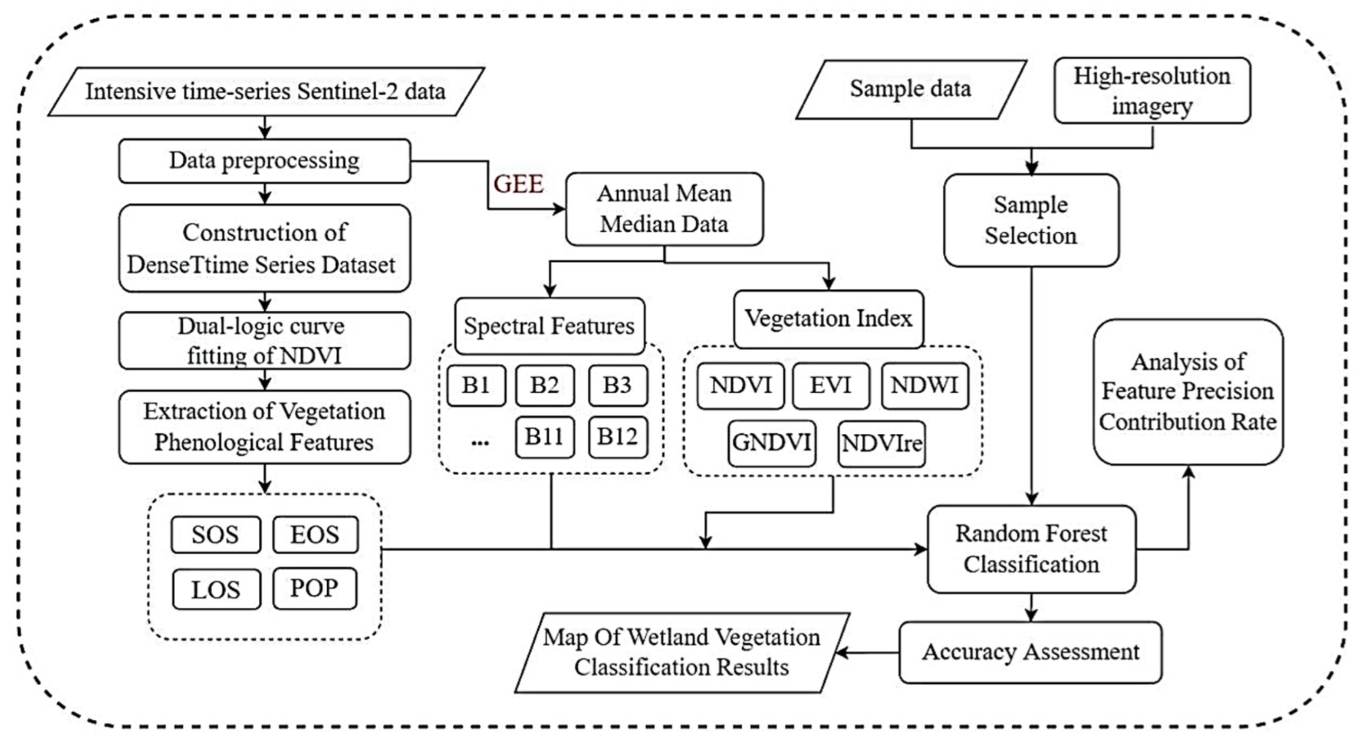
2.3. Methodology
2.3.1. Data Preprocessing
2.3.2. Construction of Dense Time-Series Dataset
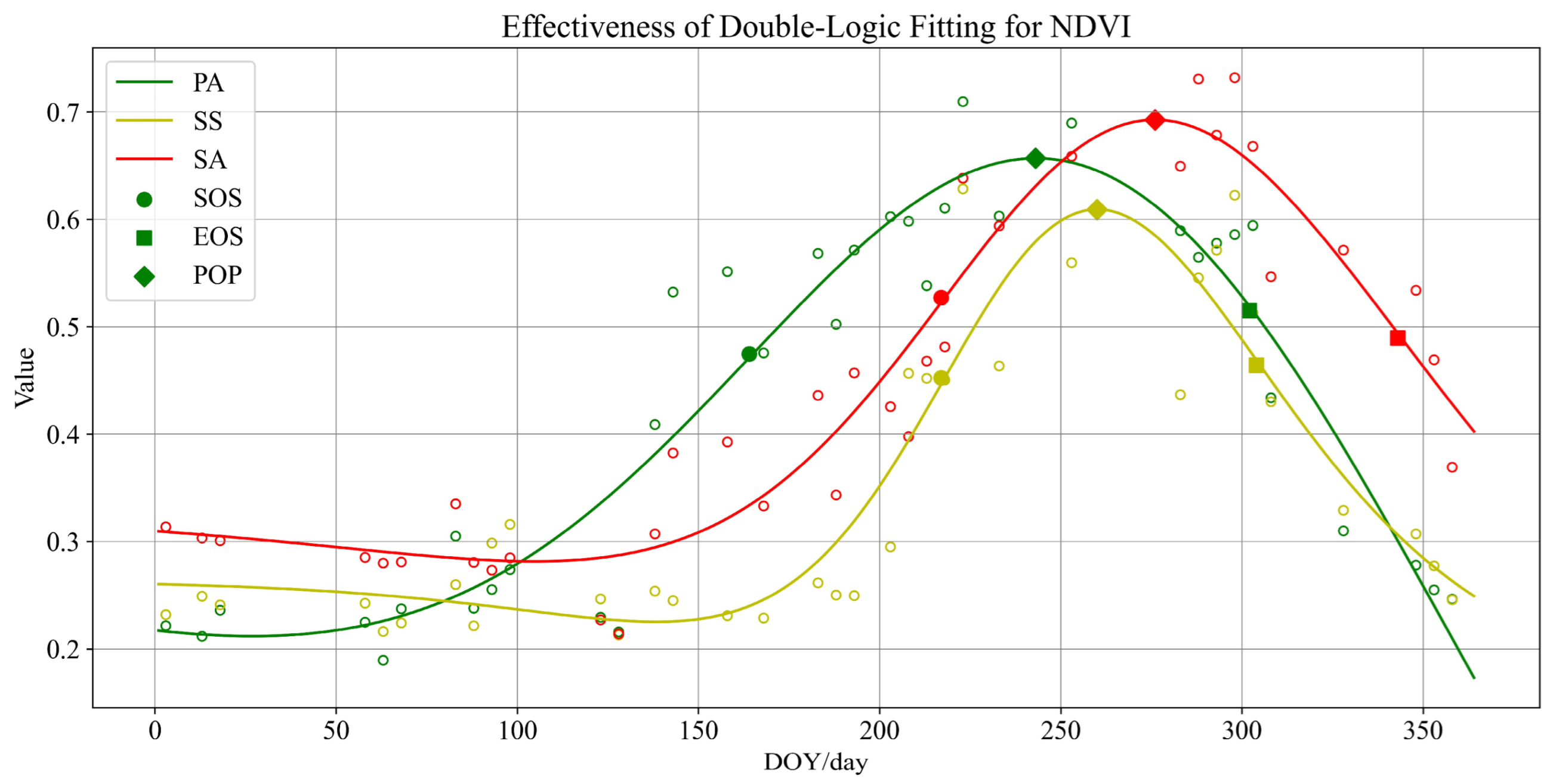
2.3.3. Extraction of Vegetation’s Phenological Features
2.3.4. Feature Fusion of Spectral Features, Vegetation Indices, and Phenological Features
2.4. Random Forest Classification (RF)
- (a)
- Use N for the number of training examples (samples) and M for the number of features.
- (b)
- Choose the number of input features (m) for determining decisions at each tree node, where m is considerably less than M.
- (c)
- Employ bootstrapping by randomly sampling N times with replacement, creating a training set, and evaluating errors on the remaining unsampled examples.
- (d)
- Randomly select m features for each node and compute optimal splitting based on these features.
- (e)
- Allow each tree to grow fully without pruning.
2.5. Accuracy Assessment
2.6. Statistical Significance of Classifiers’ Performance
3. Results and Analysis
3.1. Analysis of Available Pixel Count
3.2. Analysis of Vegetation Phenology Models’ Fitted Curves Based on NDVI
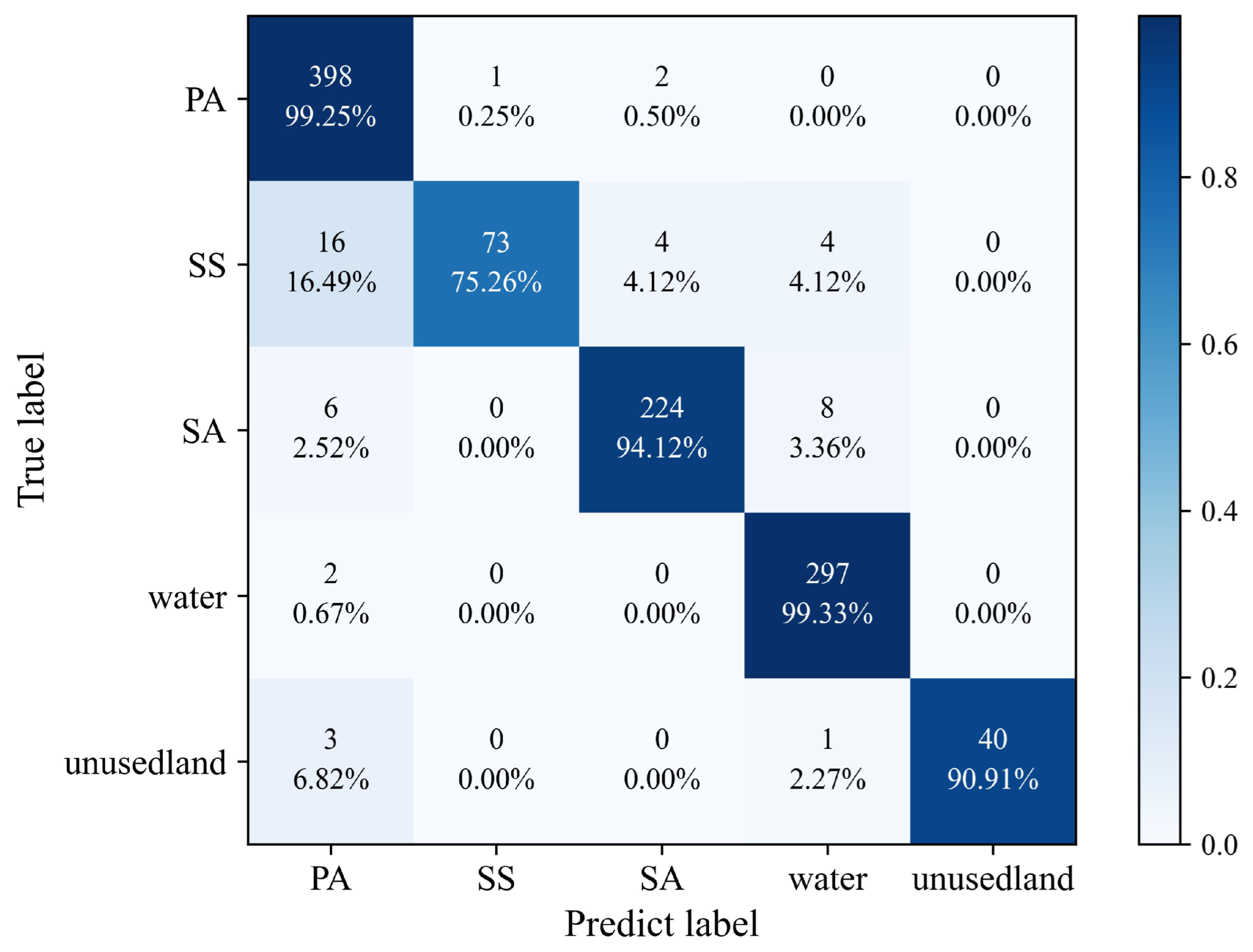
3.3. Classification Results and Accuracy Evaluation
3.4. Feature Contribution Analysis
3.5. Comparison of Multiple Feature Fusion Methods
3.6. Misclassification Analysis Based on Land-Use Change Mapping
3.7. Analysis of Misclassification Results
4. Discussion
4.1. Comparison with Previous Works
4.2. Shortcomings and Future Plans
5. Conclusions
- A classified map of the core zone of the Yancheng Wetland Rare Birds National Nature Reserve was obtained for the year 2022, with an overall classification accuracy of 95.64% and a kappa coefficient of 0.94.
- The combination of spectral features, vegetation indices, and phenological characteristics produced the highest level of accuracy in classification. POP, SOS, NDVIre, and mid-infrared bands (Band12 and Band11) were useful for the classification of coastal wetlands.
- The influence of tidal fluctuations on SA along the shoreline was not considered in this experiment. The misclassification of SA near the coastline in the categorization map was caused by its long-term submersion, partial submersion, and non-submersion. By comparing SA plants located near the coastline with those located farther away, we showed that the phenological magnitude of SA near the coastline was relatively smaller. This finding helps to explain why these plants are more likely to be misidentified as PA.
- Different regions within the core zone of the Yancheng Wetland Rare Birds National Nature Reserve exhibit different development patterns of PA. There is a potential 1–2-month disparity in growth between early- and late-growing PA. The variation in vegetation cover can be explained by different factors, such as vegetation characteristics, soil salinity, climate changes, and the intricate nature of the vegetation.
Author Contributions
Funding
Data Availability Statement
Acknowledgments
Conflicts of Interest
Appendix A

| Name | Date | Cloud Cover (%) |
|---|---|---|
| S2_SR_HARMONIZED_20220103T024121 | 3 January 2022 | 16.93 |
| S2_SR_HARMONIZED_20220108T024059 | 8 January 2022 | 29.19 |
| S2_SR_HARMONIZED_20220113T024051 | 13 January 2022 | 16.13 |
| S2_SR_HARMONIZED_20220118T024029 | 18 January 2022 | 20.87 |
| S2_SR_HARMONIZED_20220128T023949 | 28 January 2022 | 47.73 |
| S2_SR_HARMONIZED_20220227T023639 | 2 February 2022 | 4.41 |
| S2_SR_HARMONIZED_20220304T023611 | 4 March 2022 | 16.66 |
| S2_SR_HARMONIZED_20220309T023549 | 9 March 2022 | 18.62 |
| S2_SR_HARMONIZED_20220324T023551 | 24 March 2022 | 0 |
| S2_SR_HARMONIZED_20220329T023549 | 29 March 2022 | 3.76 |
| S2_SR_HARMONIZED_20220403T023551 | 3 April 2022 | 3.03 |
| S2_SR_HARMONIZED_20220408T023549 | 8 April 2022 | 1.59 |
| S2_SR_HARMONIZED_20220503T023551 | 3 May 2022 | 0.09 |
| S2_SR_HARMONIZED_20220518T023549 | 18 May 2022 | 13.98 |
| S2_SR_HARMONIZED_20220523T023601 | 23 May 2022 | 0 |
| S2_SR_HARMONIZED_20220602T023601 | 2 June 2022 | 19.08 |
| S2_SR_HARMONIZED_20220607T023549 | 7 June 2022 | 0.41 |
| S2_SR_HARMONIZED_20220617T023529 | 17 June 2022 | 35.13 |
| S2_SR_HARMONIZED_20220702T023541 | 2 July 2022 | 41.39 |
| S2_SR_HARMONIZED_20220712T023541 | 12 July 2022 | 66.25 |
| S2_SR_HARMONIZED_20220722T023541 | 22 July 2022 | 22.27 |
| S2_SR_HARMONIZED_20220727T023529 | 27 July 2022 | 30.29 |
| S2_SR_HARMONIZED_20220801T023541 | 1 August 2022 | 32.59 |
| S2_SR_HARMONIZED_20220821T023541 | 21 August 2022 | 0.07 |
| S2_SR_HARMONIZED_20220826T023529 | 26 August 2022 | 61.19 |
| S2_SR_HARMONIZED_20220910T023541 | 10 September 2022 | 73.93 |
| S2_SR_HARMONIZED_20220930T023541 | 30 September 2022 | 55.15 |
| S2_SR_HARMONIZED_20221010T023621 | 10 October 2022 | 1.52 |
| S2_SR_HARMONIZED_20221015T023649 | 15 October 2022 | 41.48 |
| S2_SR_HARMONIZED_20221020T023731 | 20 October 2022 | 34.13 |
| S2_SR_HARMONIZED_20221025T023759 | 25 October 2022 | 4.44 |
| S2_SR_HARMONIZED_20221104T023849 | 4 November 2022 | 19.96 |
| S2_SR_HARMONIZED_20221124T024029 | 24 November 2022 | 21.01 |
| S2_SR_HARMONIZED_20221214T024119 | 14 December 2022 | 11.05 |
| S2_SR_HARMONIZED_20221219T024121 | 19 December 2022 | 1.84 |
| S2_SR_HARMONIZED_20221224T024119 | 24 December 2022 | 39.70 |
References
- Duan, H.L.; Yu, X.B. Research on Dynamic Changes of Endangered Waterbird Habitats in the Yellow and Bohai Seas. Acta Ecol. Sin. 2023, 43, 6354–6363. [Google Scholar]
- Mohseni, F.; Amani, M.; Mohammadpour, P.; Kakooei, M.; Jin, S.; Moghimi, A. Wetland mapping in Great Lakes using Sentinel-1/2 time-series imagery and DEM data in Google Earth Engin. Remote Sens. 2023, 15, 3495. [Google Scholar] [CrossRef]
- Duarte, C.M.; Losada, I.J.; Hendriks, I.E.; Mazarrasa, I.; Marbà, N. The role of coastal plant communities for climate change mitigation and adaptation. Nat. Clim. Change 2013, 3, 961–968. [Google Scholar] [CrossRef]
- Hou, X.J.; Feng, L.; Cchen, X.L.; Zhang, Y. Dynamics of the wetland vegetation in large lakes of the Yangtze Plain in response to both fertilizer consumption and climatic changes. ISPRS J. Photogramm. Remote Sens. 2018, 141, 148–160. [Google Scholar] [CrossRef]
- Ning, X.G.; Chang, W.T.; Wang, H.; Zhang, H.C.; Zhu, Q.D. Wetland Information Extraction in the Heilongjiang River Basin Using Google Earth Engine and Multi-source Remote Sensing Data. J. Remote Sens. 2022, 26, 386–396. [Google Scholar]
- Chen, B.; Chen, L.; Huang, B.; Michishita, R.; Xu, B. Dynamic monitoring of the Poyang Lake wetland by integrating Landsat and MODIS observations. ISPRS J. Photogramm. Remote Sens. 2018, 139, 75–87. [Google Scholar] [CrossRef]
- Fan, D.Q.; Zhao, X.S.; Zhu, W.Q.; Zheng, Z. Review on Factors Affecting the Accuracy of Plant Phenology Remote Sensing Monitoring. Prog. Geogr. 2016, 35, 304–319. [Google Scholar]
- Liu, R.Q. Coastal Wetland Classification Based on Time Series Remote Sensing Images and Vegetation Phenological Characteristics. Master’s Thesis, Ningbo University, Ningbo, China, 2022. [Google Scholar]
- Zhang, L.; Gong, Z.N.; Wang, Q.W.; Jin, D.D.; Wang, X. Wetland mapping of Yellow River Delta wetlands based on multi-feature optimization of Sentinel-2 images. J. Remote Sens. 2019, 23, 313–326. [Google Scholar] [CrossRef]
- Zheng, H.; Chen, X.T.; Song, L.J.; Fan, J.H.; Yang, X.W.; Song, J.R.; Song, T.L.; Liu, M.Y. Research on the Extraction Method of Spartina alterniflora Information in Coastal Wetlands Based on Google Earth Engine (GEE). J. Chifeng Univ. Nat. Sci. Ed. 2022, 38, 26–31. [Google Scholar]
- Sun, W.W.; Liu, W.W.; Wang, Y.M.; Zhao, R.; Huang, M.; Wang, Y.; Yang, G.; Meng, X. Progress and Prospects of Global Wetland Hyperspectral Remote Sensing Research from 2010 to 2022. J. Remote Sens. 2023, 27, 1281–1299. [Google Scholar]
- Wu, Y.; Xiao, X.; Chen, B.; Ma, J.; Wang, X.; Zhang, Y.; Zhao, B.; Li, B. Tracking the phenology and expansion of Spartina alterniflora coastal wetland by time series MODIS and Landsat images. Multimed. Tools Appl. 2020, 79, 5175–5195. [Google Scholar] [CrossRef]
- Zhang, X.; Liu, L.; Zhao, T.; Chen, X.; Lin, S.; Wang, J.; Mi, J.; Liu, W. GWL_FCS30: Global 30 m wetland map with fine classification system using multi-sourced and time-series remote sensing imagery in 2020. Earth Syst. Sci. Data Discuss. 2022, 15, 265–293. [Google Scholar] [CrossRef]
- Chao, S.; Li, J.; Liu, Y.; Liu, Y.; Liu, Y.; Liu, R. Plant species classification in salt marshes using phenological parameters derived from Sentinel-2 pixel-differential time-series. Remote Sens. Environ. 2021, 256, 112320. [Google Scholar]
- Liu, R.Q.; Li, J.L.; Sun, C.; Sun, W.W.; Cao, L.D.; Tian, P. Vegetation Classification of Yancheng Coastal Wetlands Based on Sentinel-2 Remote Sensing Time Series Phenological Features. Acta Geogr. Sin. 2021, 76, 1680–1692. [Google Scholar]
- Tassi, A.; Vizzari, M. Object-oriented LULC classification in Google earth engine combining SNIC, GLCM, and machine learning algorithms. Remote Sens. 2020, 12, 3776. [Google Scholar] [CrossRef]
- Taddeo, S.; Dronova, I.; Depsky, N. Spectral vegetation indices of wetland greenness: Responses to vegetation structure, composition, and spatial distribution. Remote Sens. Environ. 2019, 234, 111467. [Google Scholar] [CrossRef]
- Wu, X.F.; Hua, S.H.; Zhang, S.; Gu, L.; Ma, C.; Li, C. Extraction of Winter Wheat Distribution Information Based on Multi-Phenological Feature Indices from Sentinel-2 Data. Trans. Chin. Soc. Agric. Mach. 2023, 54, 207–216. [Google Scholar]
- Gonsamo, A.; Chen, J.M.; D’Odorico, P. Deriving land surface phenology indicators from CO2 eddy covariance measurements. Ecol. Indic. 2013, 29, 203–207. [Google Scholar] [CrossRef]
- Rogers, C.; Chen, J.M.; Croft, H.; Gonsamo, A.; Luo, X.; Bartlett, P.; Staebler, R.M. Daily leaf area index from photosynthetically active radiation for long term records of canopy structure and leaf phenology. Agric. For. Meteorol. 2021, 304, 108407. [Google Scholar] [CrossRef]
- Zhang, Q.; Kong, D.; Shi, P.; Singh, V.P.; Sun, P. Vegetation phenology on the Qinghai-Tibetan Plateau and its response to climate change (1982–2013). Agric. For. Meteorol. 2018, 248, 408–417. [Google Scholar] [CrossRef]
- Wu, C.; Peng, D.; Soudani, K.; Siebicke, L.; Gough, C.M.; Arain, M.A.; Bohrer, G.; Lafleur, P.M.; Peichl, M.; Gonsamo, A.; et al. Land surface phenology derived from normalized difference vegetation index (NDVI) at global FLUXNET sites. Agric. For. Meteorol. 2017, 233, 171–182. [Google Scholar] [CrossRef]
- Prasad, P.; Loveson, V.J.; Kotha, M. Probabilistic coastal wetland mapping with integration of optical, SAR and hydro-geomorphic data through stacking ensemble machine learning model. Ecol. Inform. 2023, 77, 102273. [Google Scholar] [CrossRef]
- Wen, L.; Mason, T.J.; Ryan, S.; Ling, J.E.; Saintilan, N.; Rodriguez, J. Monitoring long-term vegetation condition dynamics in persistent semi-arid wetland communities using time series of Landsat data. Sci. Total Environ. 2023, 905, 167212. [Google Scholar] [CrossRef]
- Breiman, L. Random forests. Mach. Learn. 2001, 45, 5–32. [Google Scholar] [CrossRef]
- Genuer, R.; Poggi, J.M.; Tuleau-Malot, C. Variable selection using random forests. Pattern Recognit. Lett. 2010, 31, 2225–2236. [Google Scholar] [CrossRef]
- Congalton, R.G. Remote sensing and geographic information system data integration: Error sources and research issues. Photogramm. Eng. Remote Sens. 1991, 57, 677–687. [Google Scholar]
- Foody, G.M. Thematic map comparison. Photogramm. Eng. Remote Sens. 2004, 70, 627–633. [Google Scholar] [CrossRef]
- Agresti, A. An Introduction to Categorical Data Analysis; Wiley: New York, NY, USA, 1996. [Google Scholar]
- Congalton, R.G.; Oderwald, R.G.; Mead, R.A. Assessing Landsat classification accuracy using discrete multivariate statistical techniques. Photogramm. Eng. Remote Sens. 1983, 49, 1671–1678. [Google Scholar]
- Xing, H.; Niu, J.; Feng, Y.; Hou, D.; Wang, Y.; Wang, Z. A coastal wetlands mapping approach of Yellow River Delta with a hierarchical classification and optimal feature selection framework. Catena 2023, 223, 106897. [Google Scholar] [CrossRef]
- Hao, P.; Di, L.; Zhang, C.; Guo, L. Transfer Learning for Crop classification with Cropland Data Layer data (CDL) as training samples. Sci. Total Environ. 2020, 733, 138869. [Google Scholar] [CrossRef]


| Vegetation Indices | Calculation Formulae |
|---|---|
| NDVI | |
| GNDVI | |
| NDVIre | |
| NDWI | |
| EVI | 2.5 × ((NIR − RED)/(NIR + 6 × RED − 7.5 × BLUE + 1)) |
| Allocation | Classification 2 | ||
|---|---|---|---|
| Classification 1 | Correct | Incorrect | Sum |
| Correct | |||
| Incorrect | |||
| Sum | |||
| Classification | Scheme 1 | Scheme 2 | Scheme 3 | Scheme 4 | Scheme 5 | Scheme 6 | Scheme 7 | |||||||
|---|---|---|---|---|---|---|---|---|---|---|---|---|---|---|
| PA1% | UA% | PA1% | UA% | PA1% | UA% | PA1% | UA% | PA1% | UA% | PA1% | UA% | PA1% | UA% | |
| PA | 98.25 | 89.95 | 90.78 | 86.26 | 89.78 | 83.53 | 99.00 | 90.43 | 98.50 | 93.39 | 95.01 | 92.02 | 99.25 | 93.65 |
| SS | 75.26 | 96.05 | 72.17 | 87.50 | 46.39 | 57.69 | 73.20 | 98.61 | 79.38 | 96.25 | 64.95 | 87.50 | 75.26 | 98.65 |
| SA | 86.98 | 95.39 | 79.00 | 84.31 | 85.29 | 83.20 | 87.39 | 95.41 | 92.44 | 98.65 | 91.18 | 90.42 | 94.12 | 97.39 |
| WA | 99.00 | 96.73 | 99.00 | 93.38 | 88.29 | 88.29 | 99.33 | 96.43 | 99.67 | 95.21 | 98.66 | 93.95 | 99.33 | 95.81 |
| UN | 93.18 | 97.62 | 79.55 | 94.60 | 45.46 | 74.07 | 93.18 | 97.62 | 90.91 | 100 | 84.09 | 94.87 | 90.91 | 100 |
| OA% | 93.70 | 88.32 | 82.67 | 93.98 | 95.46 | 94.08 | 95.64 | |||||||
| Kappa | 0.91 | 0.84 | 0.76 | 0.92 | 0.94 | 0.92 | 0.94 | |||||||
| Classification 1 | Classification 2 | Z-Test | X2-Test | p-Value |
|---|---|---|---|---|
| RF with SP+VI+PH | RF with SP | 3.13 | 21.0 | =0.0029 |
| RF with SP+VI+PH | RF with VI | 7.94 | 79.0 | <0.0001 |
| RF with SP+VI+PH | RF with PH | 11.44 | 142.0 | <0.0001 |
| RF with SP+VI+PH | RF with SP+VI | 2.71 | 18.0 | =0.0104 |
| RF with SP+VI+PH | RF with SP+PH | 0.38 | 2.0 | =0.8501 |
| RF with SP+VI+PH | RF with VI+PH | 5.46 | 39.0 | <0.0001 |
Disclaimer/Publisher’s Note: The statements, opinions and data contained in all publications are solely those of the individual author(s) and contributor(s) and not of MDPI and/or the editor(s). MDPI and/or the editor(s) disclaim responsibility for any injury to people or property resulting from any ideas, methods, instructions or products referred to in the content. |
© 2024 by the authors. Licensee MDPI, Basel, Switzerland. This article is an open access article distributed under the terms and conditions of the Creative Commons Attribution (CC BY) license (https://creativecommons.org/licenses/by/4.0/).
Share and Cite
Wang, Y.; Jin, S.; Dardanelli, G. Vegetation Classification and Evaluation of Yancheng Coastal Wetlands Based on Random Forest Algorithm from Sentinel-2 Images. Remote Sens. 2024, 16, 1124. https://doi.org/10.3390/rs16071124
Wang Y, Jin S, Dardanelli G. Vegetation Classification and Evaluation of Yancheng Coastal Wetlands Based on Random Forest Algorithm from Sentinel-2 Images. Remote Sensing. 2024; 16(7):1124. https://doi.org/10.3390/rs16071124
Chicago/Turabian StyleWang, Yongjun, Shuanggen Jin, and Gino Dardanelli. 2024. "Vegetation Classification and Evaluation of Yancheng Coastal Wetlands Based on Random Forest Algorithm from Sentinel-2 Images" Remote Sensing 16, no. 7: 1124. https://doi.org/10.3390/rs16071124
APA StyleWang, Y., Jin, S., & Dardanelli, G. (2024). Vegetation Classification and Evaluation of Yancheng Coastal Wetlands Based on Random Forest Algorithm from Sentinel-2 Images. Remote Sensing, 16(7), 1124. https://doi.org/10.3390/rs16071124