Biomass Estimation with GNSS Reflectometry Using a Deep Learning Retrieval Model

Abstract

GNSS Reflectometry (GNSS-R) is an emerging technique for the remote sensing of the environment. Traditional GNSS-R bio-geophysical parameter retrieval algorithms and deep learning models utilize observables derived from only the peak power of the delay-Doppler maps (DDMs), discarding the rest. This reduces the data available, which potentially hinders estimation accuracy. In addition, reflections from water bodies dominate the signal amplitude, and using only the peak power in those areas is challenging. Motivated by all the above, we propose a novel deep learning retrieval model for biomass estimation that uses the full DDM of surface reflectivity. Experiments using CYGNSS data have illustrated the improvements achieved when using the full DDM of surface reflectivity. Our proposed model was able to estimate biomass, trained using the ESA Climate Change Initiative (CCI) biomass map, outperforming the model that used peak reflectivity. Global and regional analysis is provided along with an illustration of how biomass estimation is achieved when using the full DDM around water bodies. GNSS-R could become an efficient method for biomass monitoring with fast revisit times. However, an elaborate calibration is necessary for the retrieval models, to associate GNSS-R data with bio-geophysical parameters on the ground. To achieve this, further developments with improved training data are required, as well as work using in situ validation data. Nevertheless, using GNSS-R and deep learning retrieval models has the potential to enable fast and persistent biomass monitoring and help us better understand our changing climate.

1. Introduction

Above-ground-biomass is an essential climate variable that determines the global distribution of carbon. The recent drastic increase in CO₂ is believed to be the major factor causing climate change and the cause of the greenhouse effect [1]. Unfortunately, global in situ biomass measurements are impractical due to the vast areas to cover, as well as the inaccessibility of remote and dense tropical forests. Remote sensing is a more suitable approach, which exploits the electromagnetic wave interaction mechanisms (e.g., scattering and attenuation) with vegetation to indirectly infer the above-ground-biomass.

There have been numerous efforts to generate biomass maps using data acquired from space. LIDAR data such as NASA’s GEDI [2] and ICESat-1 (GLAS instrument) [3] missions have been used to estimate forest canopy heights and above-ground-biomass in conjunction with other instruments. However, they suffer from clouds (e.g., around tropical forests) and weather conditions, limiting their spatial extent. On the other hand, microwave signals can penetrate through clouds and operate irrespective of weather conditions. JAXA’s ALOS series missions use synthetic aperture radar systems in the L-band to measure backscatter intensity and infer above-ground-biomass. Nevertheless, it was shown that it saturates at around 100 tonnes/ha [4]. The future ESA BIOMASS mission [5] will use the P-band and aims to overcome this limitation.

At the same time, numerous studies have utilized reflected signals from the Global Navigation Satellite System (GNSS), to retrieve bio-geophysical parameters [6,7]. GNSS-Reflectometry (GNSS-R) is a multi-bistatic radar, which utilizes reflected L-band navigation signals, with as many transmitters as in-view GNSS satellites (e.g., Galileo, GPS). The spectral region of the navigation signal is sensitive to water content, and it can penetrate through vegetation. Low-cost GNSS-R passive instruments enable smaller platforms and larger constellations, translating into wide spatial coverage and high revisit times.

Several spaceborne GNSS-R missions have demonstrated the potential of this technique, from Disaster Monitoring Constellation-1 (DMC-1) [8], TechDemoSat-1 (TDS-1) [9], a specific mission mode of the Soil Moisture Active Passive (SMAP) [10], to the constellation of the Cyclone GNSS (CYGNSS) [11], the BuFeng-1 A/B constellation [12], the FSSCat [13], and commercial GNSS-R constellations such as Spire’s cubesats [14,15]. There are planned missions such as ESA’s Hydrology using GNSS reflections (HydroGNSS) [16].

Initial proposals for the utilization of GNSS-R involved ocean remote sensing [8,17,18,19], for altimetry [20,21] and wind speed retrieval [22,23]. Nevertheless, over the years, many different applications have emerged for the estimation of wind direction [24], sea target detection [25,26] and over land [27,28] such as soil moisture [29,30], and above-ground-biomass [31,32], to name a few. For an in-depth review, ref. [6] provides details for various geophysical parameters, and [7] focuses specifically on land applications.

This work investigates the application of GNSS-R over land, and more specifically, for biomass estimation. The main mechanism that enables GNSS-R data to be sensitive to biomass is the attenuation of the near-specular reflected signal from the soil due to vegetation [7]. One of the key observables is the equivalent surface reflectivity, $\Gamma$, defined in Equation (1). Figure 1a illustrates the gridded, mean $\Gamma$ (the mean is calculated from the surface reflectivity of the full DDM per specular point and then gridded at 5 km), and Figure 1b includes the corresponding above-ground-biomass (AGB) from the ESA Climate Change Initiative (CCI) [33]. It can be seen that there is a general trend when biomass is high and $\Gamma$ is low and vice versa. However, biomass estimation from GNSS-R data is a highly ill-posed problem. The received power on a GNSS-R platform depends not only on biomass, but on many other parameters and factors.

Recently, efforts have been focused on spaceborne GNSS-R data from TDS-1 and the CYGNSS constellation. The trailing edge and reflectivity derived from CYGNSS were used in [32] to study their sensitivity and ability to retrieve biomass. An empirical approach based on polynomial fitting was used to estimate biomass at selected test sites with encouraging preliminary results. Further studies augmented the GNSS-R-derived observables with other data such as latitude/longitude, the signal-to-noise ratio [31], and soil moisture [34].

The above studies utilize a single value for equivalent surface reflectivity, computed from the maximum power received at the platform for each location. This results in more than $99\%$ of the data available from the delay-Doppler map (DDM) shown in Figure 2 being discarded due to the difficulty in incorporating them into traditional retrieval algorithms. There have been studies that propose to use the full DDM to extract additional information using deep learning models for soil moisture estimation [35] and wind speed retrieval [36]. Before moving further, it is worth providing more details and characteristics, motivating the use of the full DDM for biomass estimation.

Over land surfaces, the reflected GNSS signal is composed of a nearly specular reflection from the soil surface and diffuse scattering for vegetation and surface roughness [31]. This means that the signal is composed of both coherent and incoherent scattering, with the relative portion depending on the coherent integration time, the acquisition geometry, and the properties of the scattering media [32]. The type of scattering is important as it affects the spatial resolution achievable by the instrument. It is approximately determined by the size of the first Fresnel zone for coherent scattering (hundreds of meters) [37] or about 25 km for incoherent scattering [6]. This results in the signal arriving from a limited zone around a specular point (pre-defined based on the instantaneous acquisition geometry) where the power is the strongest, called the glistening zone. Note that the contribution of each type of scattering is yet to be fully understood and remains an open research question in the GNSS-R community [7].

From this zone, the main product is the delay-Doppler map (DDM). A cross-correlation of the received data with a clean replica of the PRN code [6] is performed for different delays (difference in traveling path) and carrier frequency offsets (frequency shift of scattered signal) to compute a map of power across these spatial dimensions. The structure within the DDMs is different depending on the observable scene on Earth; however, it is challenging to quantify these differences in closed form. Figure 2 illustrates three examples of DDMs. It can be seen that, as the biomass changes on the ground, the DDM structure changes. In addition, with increasing biomass, the peak power decreases.

By using the peak power alone, the additional information from the structure of the DDMs is not utilized. Not only that, if the observation area contains water bodies, it would make the peak power of the GNSS-R signal unusable. This is because the power of the reflection over water dominates the amplitude of the reflected signal [35]. Motivated by this and the differences in the structure of the DDMs with varying biomass values, we propose to utilize the full DDM for biomass estimation. We developed a novel deep learning retrieval model that utilizes the equivalent surface reflectivity from the full DDMs for biomass estimation with single-pass retrieval, that is the GNSS-R data are not gridded prior to estimation, providing greater flexibility. We also performed correlation analysis and filtering recommendations for the generation of training data, as well as ablation studies for the choice of inputs. This resulted in a deep learning retrieval model that is able to estimate biomass using only input data related to the GNSS-R acquisition, independent of any external sources.

The rest of the paper is organized as follows: Section 2 describes the generation of the training data and the deep learning retrieval model. Section 3 provides the description of the experiments and results. Lastly, Section 4 analyses and discusses the results of the study.

2. Materials and Methods

In this section, the data used and the procedure to curate a training dataset is provided. Then, the proposed deep learning retrieval model is described.

2.1. Training Data Generation

In order to create a dataset that is suitable for training deep learning models for GNSS-R, there are several steps that need to be performed. The appropriate inputs and the corresponding target need to be selected, studied, and co-located.

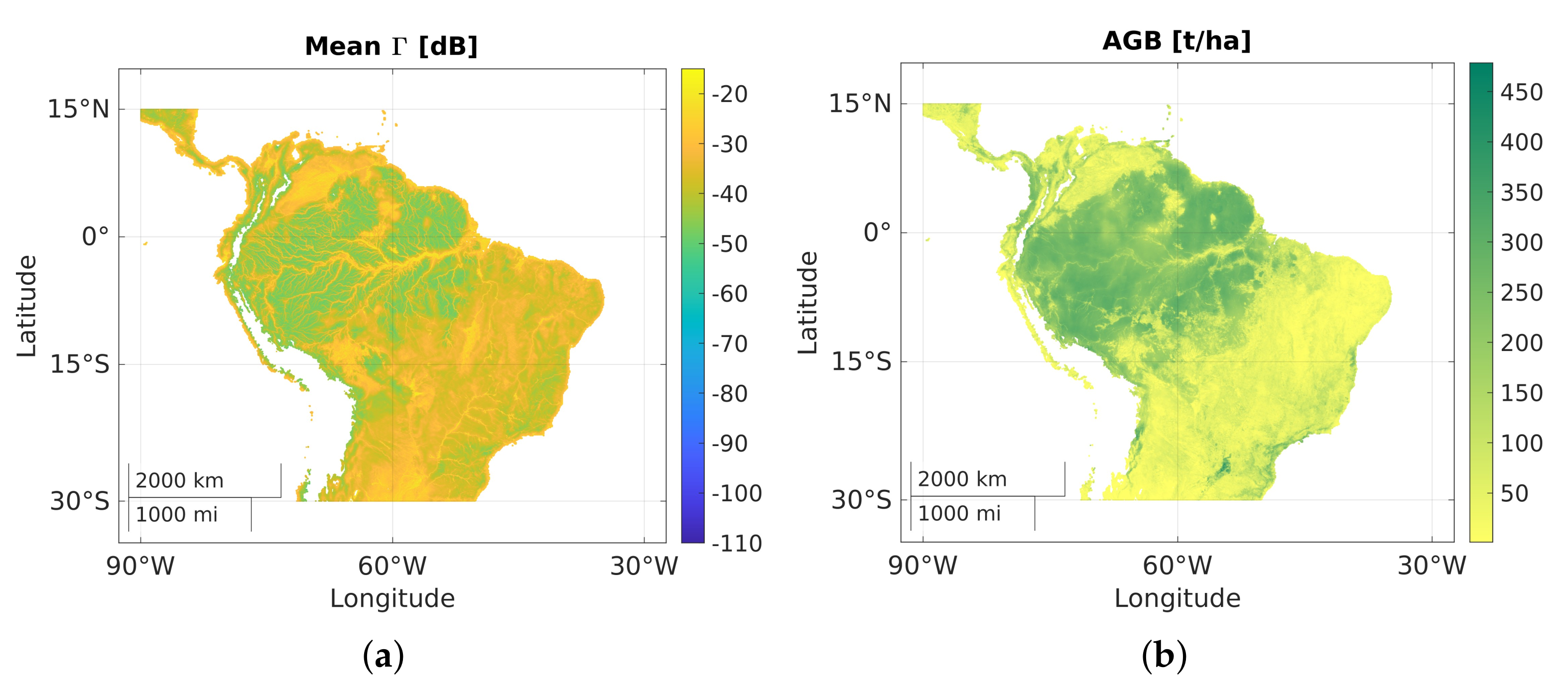
2.1.1. CYGNSS Dataset

The CYGNSS mission is a constellation of eight small satellites, each of which collects forward-scattered navigation signals from four specular points simultaneously. The measurements are limited to $\pm 38$ degrees latitude since it was originally designed to track wind speeds and extreme events such as cyclones in the tropics. The data are accessible via the Physical Oceanography Distributed Active Archive Center (PODAAC) [38].

Level 1 delay-Doppler maps (DDMs) from the v3.0 dataset have been extracted from the database. As illustrated in Figure 2, this is a $17\times 11$ element array of calibrated power in Watts. Each sample in the DDM corresponds to the power received at a certain delay and Doppler shift. Along with the DDMs, some informative data are also provided. These could be used as additional inputs to the retrieval algorithm or utilized for computing other observables. Among the main observables that have shown sensitivity to biomass are: the DDM, the signal-to-noise ratio (SNR), and the equivalent surface reflectivity, $\Gamma$ [31,32]. The latter embeds the effects of surface moisture content, small-scale roughness, and attenuation introduced by vegetation cover [7]. The SNR is available from the L1 files, and it is the ratio of the maximum value of the uncalibrated DDM in raw counts over the average per-bin raw noise counts. On the other hand, $\Gamma$ is computed using Equation (1):

$$\Gamma =\frac{{\left(4\pi \right)}^2{P}_{\mathrm{ddm}}{(R_t+R_r)}^2}{{\lambda }^2{G}_r{G}_t{P}_t},$$

(1)

where $P_{\mathrm{ddm}}$ is a sample from the $17\times 11$ power DDM, $R_t$ is the distance from the specular point and the transmitter, $R_r$ is the distance from the receiver to the specular point, $\lambda$ is the wavelength of the GPS L1 signal, $G_r$ is the receiver antenna gain in the direction of the specular point, and $G_t{P}_t$ is the transmitter equivalent isotropically radiated power (EIRP). All quantities are provided in the L1 files and are used for the calibration of the power from the full DDM to the equivalent surface reflectivity per specular point.

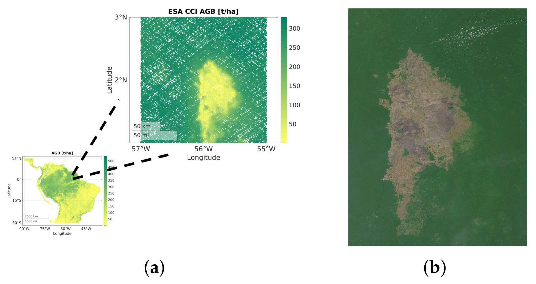
2.1.2. ESA CCI Biomass Map

The European Space Agency Climate Change Initiative (ESA CCI) provides yearly datasets of biomass maps up to 2020, at the time of writing [33], including some that coincide with the period that the CYGNSS mission has been active. The ESA CCI biomass is derived by utilizing a variety of data sources depending on the year, including Copernicus Sentinel-1, Envisat’s ASAR, and JAXA’s ALOS series, and rely on allometries from NASA’s GEDI and ICESat-2 missions.

It is worth noting that the ESA CCI biomass maps are static, and there is one map for the entire year. The map does not provide any evolution over time, which is not the optimal reference when using a time series of GNSS-R data acquisitions [7]. However, in the absence of any other easily accessible reference dataset in the desired spatial resolution, it was chosen for training and testing data as a proof-of-concept.

The original spatial resolution of the biomass maps is 100 meters per pixel, while the resolution of the CYGNSS data is expected to be lower. Based on previous studies [31] and the expected resolution in a regime of GNSS-R incoherent scattering (which is the predominant type of scattering in the presence of biomass), we selected 5 km as the biomass spatial resolution. To do that, we averaged the original 100-meter ESA CCI biomass pixels around 5 km of each specular point and co-located them with the corresponding CYGNSS data acquisition. Figure 3 includes the ESA CCI biomass maps for 2019 and 2020.

2.2. Correlation Analysis and Data Filtering

There are numerous inputs that could be derived from the CYGNSS data. Here, we investigate the relationship of five variables with the ESA CCI biomass map at 5 km spatial resolution. These are namely the following:

1.

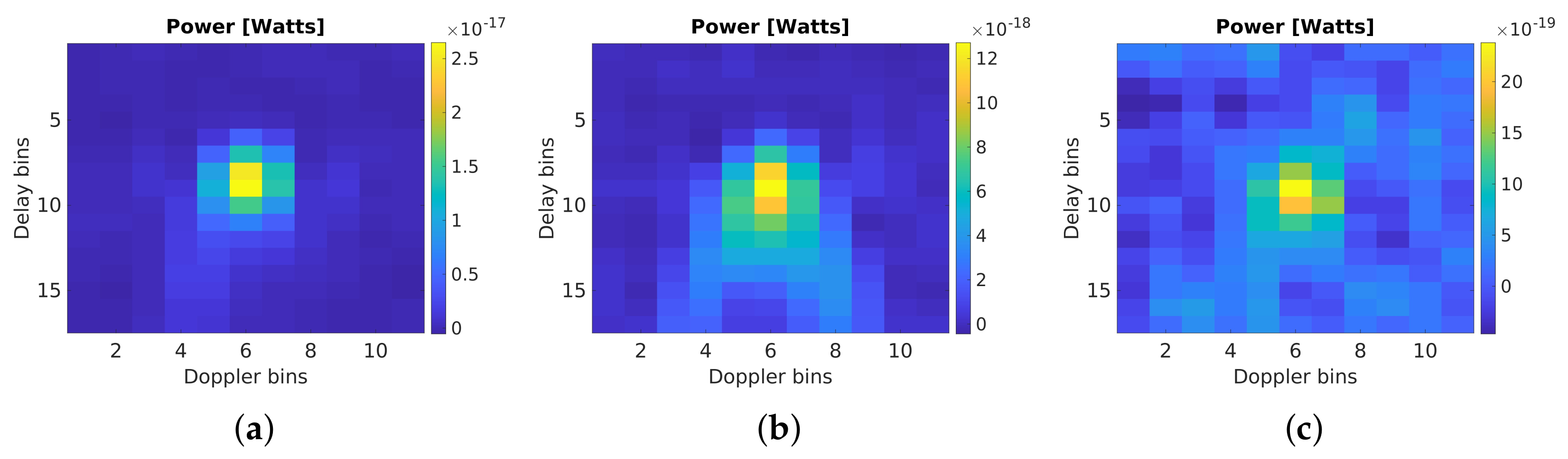
The peak power of the delay-Doppler map (DDM);

2.

The mean power of the DDM;

3.

The peak equivalent surface reflectivity per specular point;

4.

The mean equivalent surface reflectivity per specular point;

5.

The signal-to-noise ratio (SNR) per specular point.

The CYGNSS constellation produces an enormous amount of data per year. However, there might be data acquisitions with erroneous or undesirable measurements (e.g., radio frequency interference, acquisition over mountains). Thus, appropriate data filtering is required. First, measurements over the oceans and measurements with associated zero above-ground biomass are removed. Then, the surface topography of each data acquisition is considered, since it is known that CYGNSS acquisitions over regions with high elevation have performance issues [30,39]. Using the 1 km gridded digital elevation model (DEM) data from the NOAA Global Land One-km Base Elevation Project (GLOBE) [40], we filtered out all CYGNSS data acquired over regions with 2 km and above in elevation.

Furthermore, the incidence angle can affect the shape and cause distortions on DDMs; thus, acquisitions with angles outside 30–50° were discarded. Another consideration is the antenna receiver gain towards the direction of the specular point [39], which should be high enough to obtain a measurement of sufficient quality. We used data that have an associated receiver antenna gain above 3 dB. The antenna gain is provided in the CYGNSS L1 files, for the specular point only, and consideration is required of how this might affect the computation of the full DDM of reflectivity. Lastly, the radio frequency interference (RFI) needs to be considered. Using the CYGNSS RFI flag would result in substantial data reduction [35]. Therefore, we followed the approach in [35] and used custom quality filters.

Five months of the first half of 2019 were filtered as described above.

Table 1. Correlation of five GNSS-R observables with ESA CCI biomass at 5 km spatial resolution.

Variable/Res.	5 km
Samples	$\mathbf{13}.\mathbf{9}\times {\mathbf{10}}^{\mathbf{6}}$
Max DDM	−0.36173
Mean DDM	−0.44531
Max $\Gamma$	−0.37602
Mean $\Gamma$	−0.47389
SNR	−0.28362

lists the correlation coefficient between the five observables of interest and the ESA CCI biomass. It can be seen that the observable with the best indicator is the mean equivalent surface reflectivity, $\Gamma$. The second-best observable is the mean power of the DDM. This re-enforces our motivation to use information from the full DDM as opposed to its maximum power.

2.3. Deep Learning Model for Biomass Retrieval

Incorporating the full DDM into traditional retrieval models is not straight-forward due to the lack of closed-form expressions. However, deep learning models can process the data directly and extract features. In order to achieve this, the 2D-DDM of equivalent surface reflectivity is flattened and concatenated with additional data of interest. The concatenated vector is denoted here as $\mathbf{x}$, given by

$$\mathbf{x}=[\gamma ,x_{\mathrm{SNR}},x_{\mathrm{LAT}},x_{\mathrm{LON}},x_{\mathrm{Angle}}]$$

(2)

where $\gamma$ is the flattened surface reflectivity. $x_{\mathrm{SNR}}$ is the signal-to-noise-ratio (SNR), $x_{\mathrm{LAT}},x_{\mathrm{LON}}$ are the latitude and longitude of each specular point, and $x_{\mathrm{Angle}}$ is the incidence angle. All these variables are scalars per acquisition, available only for the specular point, and were obtained from the CYGNSS L1 files. Note that there are no inputs used that depend on any external datasets (e.g., digital elevation model or soil moisture products). The choice of the input data and the order that they are arranged were chosen empirically. Their impact on prediction accuracy is analyzed in the next section, but a more sophisticated way of selecting and arranging this vector is subject to future developments.

The concatenated vector is passed through a series of fully connected layers, in order to estimate the biomass at each location. The output of the first layer of the fully connected network is given by

$${\alpha }_0=\sigma (\mathbf{x}{\mathbf{W}}_0^T+{\mathbf{c}}_0).$$

(3)

where $\sigma$ is the sigmoid function, ${\mathbf{W}}_0$ are the weights to be learned, and ${\mathbf{c}}_0$ is a bias term. In a similar manner, the intermediate layer outputs are given by activation vectors:

$${\alpha }_l=\sigma ({\alpha }_{l-1}{\mathbf{W}}_l^T+{\mathbf{c}}_l),\forall l\in \{1,...,L-1\}.$$

(4)

The final layer estimates the biomass prediction:

$$\widehat{b}={\alpha }_{L-1}{\mathbf{w}}_L^T+c_L$$

(5)

where ${\alpha }_{L-1}$ is the output of the activation of the ($L-1$) layer, ${\mathbf{w}}_L$ are the weights to be learned, and $c_L$ is a scalar bias term. ${\mathbf{w}}_L$ is a vector, since the output is a single scalar value.

Figure 4 illustrates a schematic of the proposed deep learning retrieval model. This is analogous to traditional geophysical parameter-retrieval models, where the weights of a linear combination of selected variables are optimized via regression analysis. In the case of our model, the relationship can be non-linear using activation functions, the incorporation of new inputs and full DDMs is trivial and the number of weights to be optimized can be orders of magnitude larger. To learn the weights, we used the absolute error, given by

$$\mathcal{L}(\widehat{b},b)=|\widehat{b}-b|,$$

(6)

where b is the ESA CCI biomass value and $\widehat{b}$ is the biomass estimated by the deep learning retrieval model defined in Equation (5). Gradients of the loss with respect to each weight are calculated, and optimization is performed using the ADAM optimizer. Mini-batches are used, and optimization is performed using millions of samples as described next. All experiments were performed using the PyTorch library, version 1.10 [41].

3. Results

The ESA CCI provides static, yearly biomass maps; hence, we gathered one year of CYGNSS data acquisitions to train over the entire period and test over another year. The year of the training data is 2019, and the year of the test data is 2020. After data filtering, 49 million DDMs with their associated metadata and biomass were used for training and approximately 65 million, 6 hundred thousand DDMs for testing.

3.1. Model Capacity

In theory, neural networks could learn to approximate arbitrary functions and, thus, should be able to learn a mapping from the surface reflectivity to biomass. This is possible provided that sufficient and representative data are available and that the size of the model is chosen accordingly. Too big a model could overfit the data, too small a model might fail to learn the mapping. In this study, we chose to fix the number of the fully connected layers to four and only varied the number of neurons per layer. This was performed to better understand the model capacity required to capture the complexity of the functional mapping.

Table 2. Global prediction accuracy, computed from L2 retrievals (i.e., not gridded) using four layers.

Number of Neurons per Layer	R	RMSE
8	0.871	41.952
16	0.891	38.833
32	0.922	32.873
64	0.931	31.125
128	0.940	28.897
256	0.946	27.575

lists the global prediction accuracy, computed from L2 retrievals (i.e., not gridded) and averaged over all test samples. As the number of neurons increases, the correlation coefficient (R) between the prediction and the ESA CCI biomass map increases and the root-mean-squared error (RMSE) decreases. However, the improvement in prediction accuracy diminishes with increasing neurons, and doubling the number of neurons increases the training and inference time. Thus, we selected the model with 128 neurons per layer as a trade-off between prediction accuracy and computational load.

3.2. Ablation Study of Input Options

After choosing the model capacity, the next step is to understand the importance of various inputs to the network. For each set of inputs, a dedicated deep learning model was trained using the 2019 data and then tested over the 2020 data. The mean equivalent surface reflectivity is shown in Figure 5a and the corresponding ESA CCI biomass in Figure 5b.

First, the latitude and longitude of the CYGNSS acquisitions are used as input to enable the models to learn regional biomass patterns and behaviors. Nevertheless, location alone is not sufficient, as seen in Figure 5c, which includes the biomass estimation from a model trained using only latitude and longitude as the inputs. It can be seen that the prediction is very coarse, completely missing the small-scale variations. From Table 1, it was shown that CYGNSS observables correlate with biomass. To test if these are sufficient, we trained a model using $\Gamma$ from the full DDM, SNR, and incidence angle as inputs. Using these was not sufficient, as illustrated in Figure 5d. The model captures the smaller scales, as opposed to the model that uses only location, but does not produce an overall accurate map.

In order to exploit the best of both configurations, we trained a model using both the CYGNSS observables and the latitude and longitude. Figure 6a shows the prediction of this model, illustrating that it is possible to simultaneously capture small scales and larger regional patterns. Another input configuration of interest is the peak of the DDM scaled to the equivalent surface reflectivity. This was also shown to be correlated with biomass, and it is used in other studies as the input to neural networks for biomass estimation [31]. We trained a model using the peak reflectivity as the input as opposed to reflectivity from the full DDM, but kept the rest of the inputs the same. Figure 6b includes the biomass estimation using this model. It can be seen that the model focuses more on smaller scales, e.g., rivers are more visible, which can also be seen as higher absolute error for the model using the peak reflectivity in Figure 6d, as opposed to Figure 6c, illustrating the error using reflectivity from the full DDM.

Furthermore,

Table 3. Ablation study over the 2020 test data, computed from L2 retrievals (i.e., not gridded).

Inputs	R	RMSE
Full $\Gamma$, SNR, LAT, LON, $\theta$	0.940	28.897
Peak $\Gamma$, SNR, LAT, LON, $\theta$	0.935	29.956
LAT, LON	0.925	32.350
Full $\Gamma$, SNR, $\theta$	0.653	65.733

lists the R and RMSE of different models using various input configurations. The best configuration uses the reflectivity computed from the full DDM, SNR, and incidence angle ($\theta$) and, in addition, includes the location information. Note that the R and RMSE highlight the best model, but the small differences between the metrics do not capture the visual differences that can be seen in Figure 5 and Figure 6. Other more specialized quality metrics during model evaluation are essential in order to better understand their ability to capture spatial variations and patterns accurately.

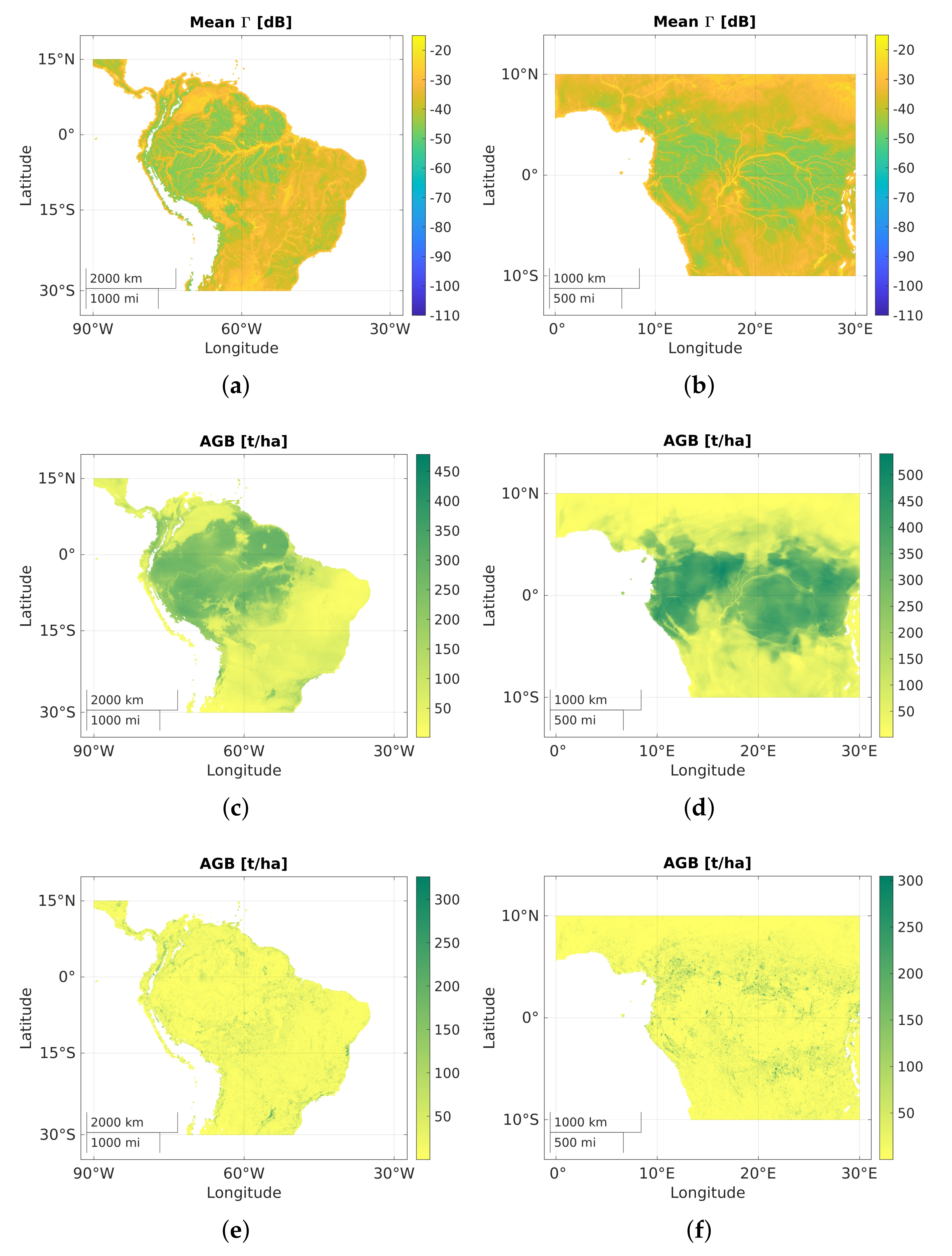
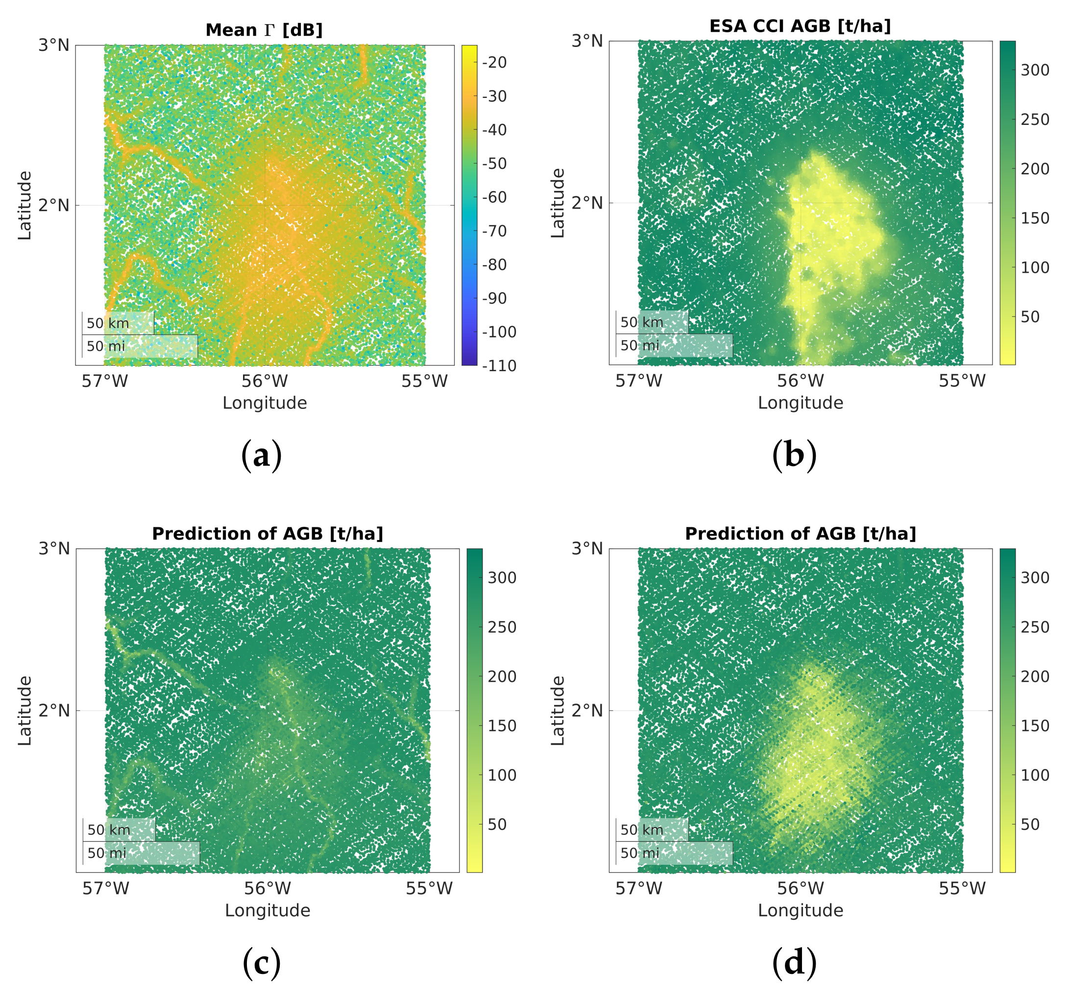
3.3. Local Analysis to Compare Full and Peak Equivalent Surface Reflectivity

We further explored the differences between the models that use the peak and full $\Gamma$ as the input, by performing a local analysis. We selected a large area around the border of Suriname and Brazil near the Sipaliwini savanna nature reserve. This is a diverse area consisting of a savanna, surrounded by a rainforest and rivers, which provides different conditions for testing biomass estimation. Figure 7a includes a zoom-in of the biomass map, with Figure 7b showing a collection of optical images captured by Sentinel-2. Low biomass in the savanna is surrounded by high biomass from the dense rainforest with rivers. The rivers are visible in the mean $\Gamma$ per specular point, as seen in Figure 8a with the associated ESA CCI biomass in Figure 8b. The peak $\Gamma$ is more sensitive to water content than the full DDM, since water bodies dominate the amplitude of the reflection [35]. The reflectivity over water is high, but this also occurs when low biomass values are present. This makes the distinction between the two wave interaction mechanisms challenging when only the peak reflectivity is available. Figure 8c illustrates the biomass estimation of the model using the peak reflectivity as the input.

Low biomass is estimated when high reflectivity occurs due to the rivers, in contrast to the ESA CCI biomass map. In addition, the low biomass over the savanna is over-estimated, which could be due to the surrounding area which has high biomass. Figure 8d includes the biomass estimation using reflectivity of the full DDM as input. The biomass is closer to the ESA CCI biomass, illustrating, for this scenario, that it is possible to overcome the issue of water bodies by using the equivalent surface reflectivity from the full DDM as the input.

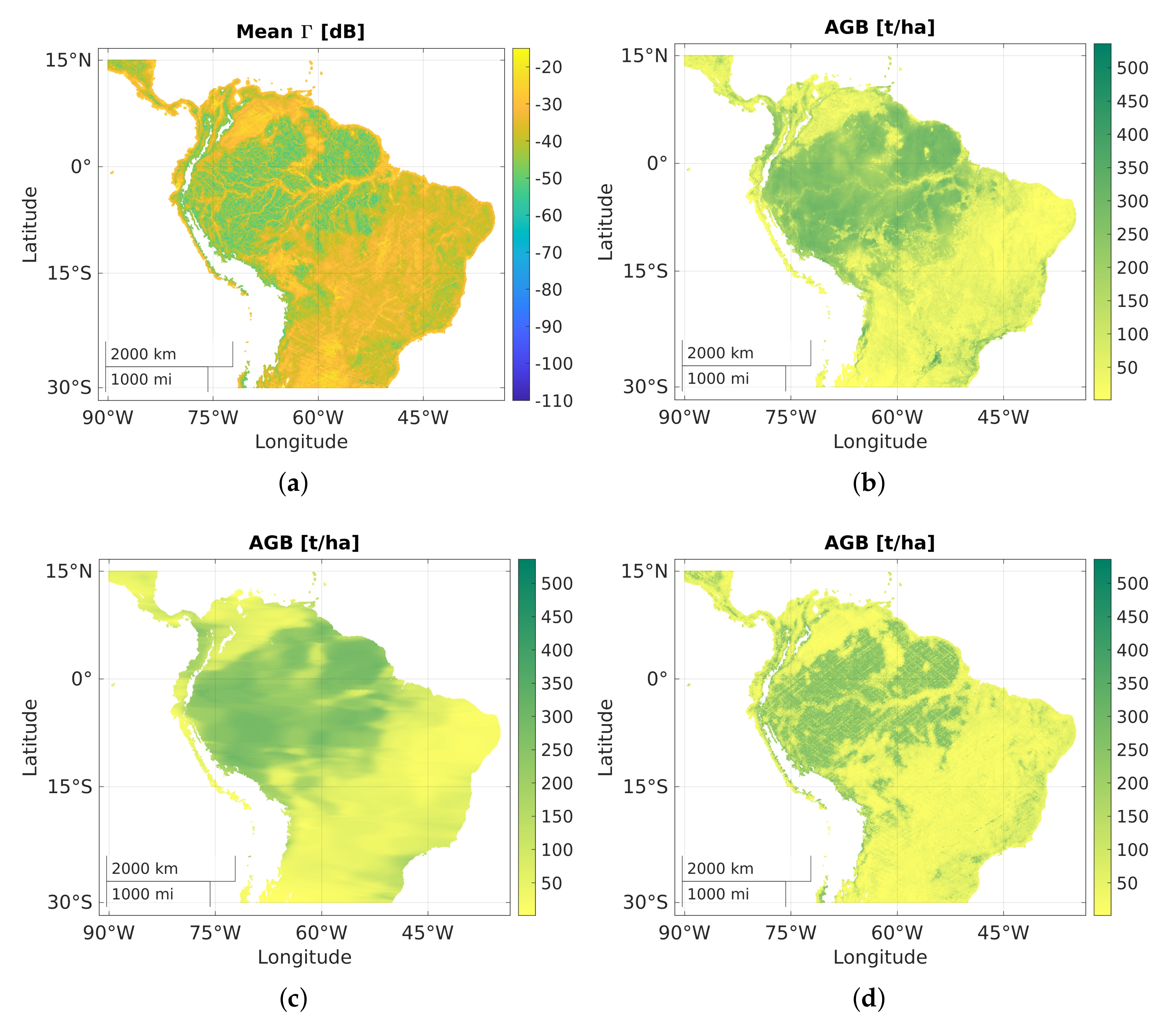
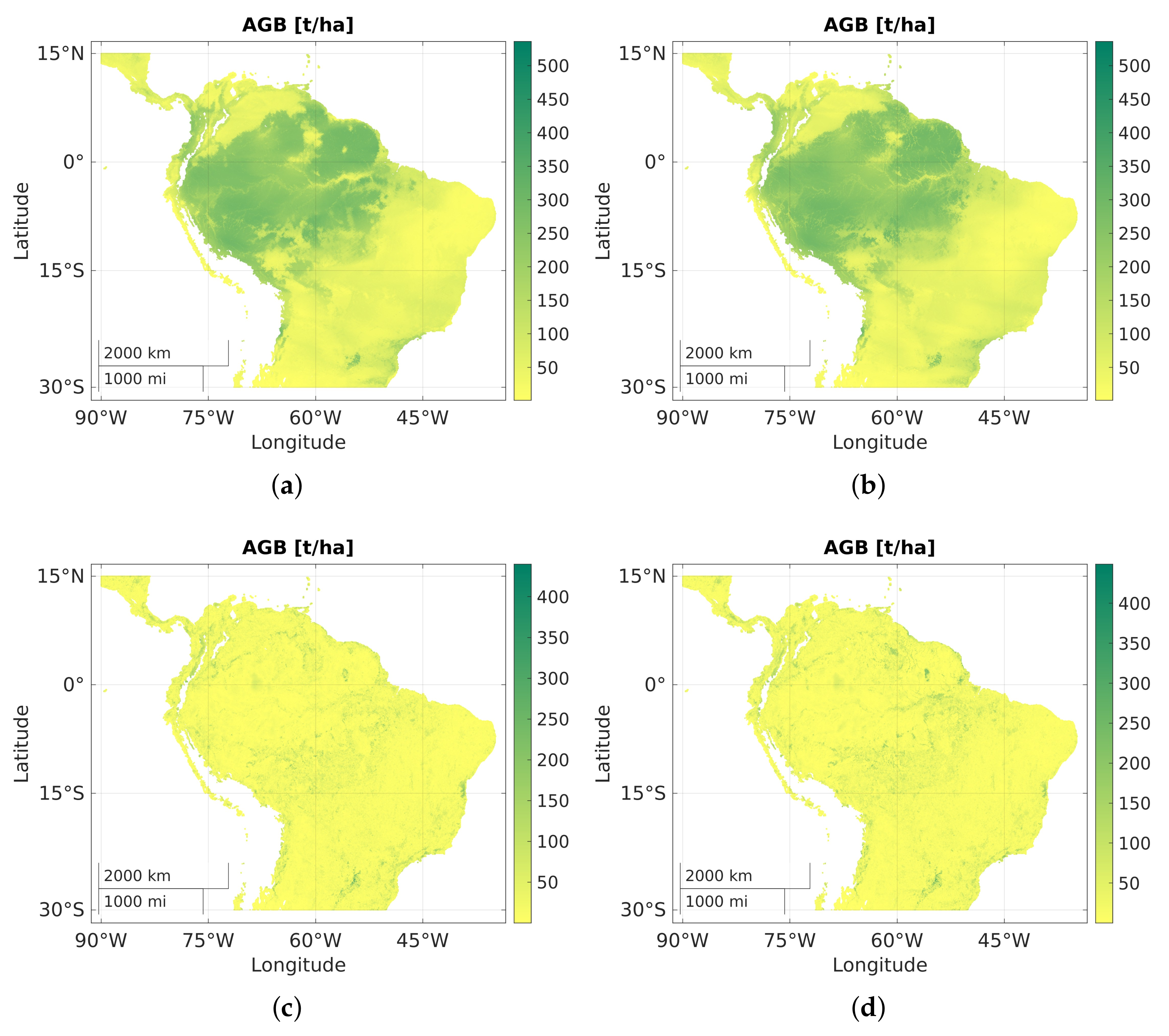
3.4. Gridding and Global Evaluation

The CYGNSS data are acquired over tracks that can vary at every pass, resulting in gaps, as seen in Figure 8. In other studies, peak reflectivity is gridded and neural network training follows. In our case, it is not trivial to grid full DDMs, thus, training was performed directly using locations of the CYGNSS acquisitions, providing also more flexibility. After estimating biomass at all locations, it is possible to aggregate them in space over 5 km areas. Figure 9a,b include the gridded mean reflectivities over South America and Central Africa, respectively, and Figure 9c,d the biomass estimations for 2020.

The absolute error differences between the biomass estimations and the ESA CCI target map are provided in Figure 9e,f. In order to understand the overall performance of our deep learning retrieval model, Figure 10a includes the global biomass estimations and Figure 10b the corresponding absolute error between the estimation and the ESA CCI biomass map. We can see that, generally, the majority of errors occur when there are sudden changes in the biomass levels. Figure 11a includes a plot of the model predictions against the ESA CCI biomass target, illustrating a very high correlation between them with a low RMSE. In addition, the histograms of the ESA CCI biomass and the predictions are provided in Figure 11b, showing a very good alignment.

4. Discussion

In this study, a deep learning retrieval model that utilizes reflectivity computed from the full DDMs is proposed and analyzed. By exploiting the differences in the DDMs when biomass values vary, more information is available to the model. This reduces the dependency on external data sources such as digital elevation models and soil moisture products. In addition, the estimation is not affected as much by surface water bodies compared to models that use the peak reflectivity. It was shown that the biomass estimated by our model has very high correlation with the ESA CCI biomass when using the reflectivity computed from the full DDM as the input, and better results can be obtained compared to peak reflectivity. Global and regional analysis illustrated the potential of our deep learning retrieval model.

Nevertheless, there are some key limitations that still need to be addressed to enable accurate and reliable biomass estimations. As was described, a deep learning retrieval model is a functional mapping with optimizable weights. The neural network architecture design is important and should be tailored to each problem, but it is adjustable and could learn arbitrary functions, if desired. The training data used to optimize it are not generally considered as being part of the model formulation. However, the model is essentially constructed by the data, and thus, the data should also be considered as integral to the model as the model itself.

For biomass estimation using GNSS-R, one of the biggest limitations is the training data used for the deep learning retrieval model. The input GNSS-R DDMs are a time series of reflectivity that vary over time, whereas the ESA CCI biomass target is static irrespective of the acquisition time. Future investigation using time-evolving biomass datasets is essential in order to assess whether the model is able to detect biomass changes reliably over time. In addition, the biomass dataset was compiled by using indirect measurements from satellites. Both of these characteristics make the target dataset not ideal, and models that are trained using these pairs of data are prone to errors. In situ datasets would be ideal, but the mismatch in spatial resolution is very big. We would need to collect in situ measurements (over an area of $5\times 5$ km) to match it to a single GNSS-R acquisition, then repeat this for a substantial amount of acquisitions to construct a training dataset.

One potential dataset that could meet at least one of the requirements is the data obtained by the NASA GEDI mission. It provides biomass estimations over time and could be aligned with GNSS-R data acquisitions for training. Future missions such as the ESA BIOMASS P-band SAR mission could also be another promising option. Moreover, potential in situ measurements from persistent forest monitoring campaigns could be exploited for cal/val purposes, if they fall within the GNSS-R data acquisition footprints. Further developments and investigations on training data and in situ cal/val data are essential such that reliable deep learning retrieval models for biomass estimation could be constructed.

Evaluating the biomass estimations and comparing with different techniques and inputs is not trivial. Traditional metrics such as the correlation coefficient and root-mean-squared error can give an indication of estimation accuracy, but they are not sufficient. By visualizing biomass estimations regionally, small scales are not always captured, although these traditional metrics would still hint at high accuracy. Specialized quality metrics that capture spatial variations are crucial for better model construction and evaluation.

During the construction of both the training data and the deep learning retrieval model, many choices are required. Data filtering is essential such that quality data are used, but at the same time, too aggressive filtering could significantly reduce the data samples. Further investigation of various data filtering options would be advantageous, as well as evaluating models with test data that fail the filtering criteria of the data used to train them. Using different cost functions and other neural network architectures would also be beneficial, in order to maximize the predictive capabilities of the models.

To compute the reflectivity from the full DDM, the antenna gain is used. However, this is provided, in the CYGNSS L1 files, only for the specular point. Part of the biomass estimation error could be caused by the fact that the surface reflectivity of the full DDM is computed using values at the specular point. Further work on this is needed to understand its impact on the biomass estimation. Another consideration is the construction of different models for different regions. Investigating whether it is useful to train dedicated models, e.g., for South America using only training data from that region and comparing it with a global model would be advantageous.

Water bodies are strong contributors to the amplitude of the reflection, dominating the GNSS-R signal with high reflectivity values. Low biomass also provides high reflectivity values, and it is challenging to distinguish between the two. By using the full DDMs, we illustrated a regional example where we were able to mitigate this effect as opposed to using the peak reflectivity. Further investigation of this is required using different scenarios to understand the limitations of the full DDM over water bodies. Moreover, water masks have been used in the past [35] as input to neural networks to help overcome this. It would be beneficial to investigate whether incorporating this would help or impact the biomass estimations in a different way.

5. Conclusions

A deep learning retrieval model that incorporates the full DDM of surface reflectivity was proposed. Experiments using CYGNSS data and the ESA CCI biomass map illustrated that it was possible to estimate biomass globally, with small errors from the biomass target used. By incorporating the full DDMs of surface reflectivity in a deep learning retrieval model, biomass estimation was more accurate than when using the peak reflectivity as the input. The full DDMs provide more information to the model, reducing the need for external data sources and making it more robust to reflections from water bodies. A constellation of GNSS-R satellites is a fast and efficient way to cover the gap in monitoring biomass with very frequent revisit times. This comes at a cost with a main hurdle that still needs to be overcome. That is, the requirement of an elaborate calibration process of the retrieval models to relate the GNSS-R data to bio-geophysical parameters on the ground. However, using GNSS-R and deep learning retrieval models has the potential to enable cost-reduced, fast, and persistent global monitoring of bio-geophysical parameters and help us understand our changing climate.

References

1. IPCC. 2023: Climate Change 2023: Synthesis Report. In Contribution of Working Groups I, II and III to the Sixth Assessment Report of the Intergovernmental Panel on Climate Change; Core Writing Team, Lee, H., Romero, J., Eds.; IPCC: Geneva, Switzerland, 2023; pp. 35–115. [Google Scholar] [CrossRef]
2. Dubayah, R.; Blair, J.B.; Goetz, S.; Fatoyinbo, L.; Hansen, M.; Healey, S.; Hofton, M.; Hurtt, G.; Kellner, J.; Luthcke, S.; et al. The Global Ecosystem Dynamics Investigation: High-resolution laser ranging of the Earth’s forests and topography. Sci. Remote Sens. 2020, 1, 100002. [Google Scholar] [CrossRef]
3. Healey, S.; Hernandez, M.; Edwards, D.; Lefsky, M.; Freeman, J.; Patterson, P.; Lindquist, E.; Lister, A. CMS: GLAS LiDAR-Derived Global Estimates of Forest Canopy Height, 2004–2008; ORNL DAAC: Oak Ridge, TN, USA, 2015. [Google Scholar] [CrossRef]
4. Baghdadi, N.; Le Maire, G.; Bailly, J.S.; Osé, K.; Nouvellon, Y.; Zribi, M.; Lemos, C.; Hakamada, R. Evaluation of ALOS/PALSAR L-Band Data for the Estimation of Eucalyptus Plantations Aboveground Biomass in Brazil. IEEE J. Sel. Top. Appl. Earth Obs. Remote Sens. 2015, 8, 3802–3811. [Google Scholar] [CrossRef]
5. Le Toan, T.; Quegan, S.; Davidson, M.; Balzter, H.; Paillou, P.; Papathanassiou, K.; Plummer, S.; Rocca, F.; Saatchi, S.; Shugart, H.; et al. The BIOMASS mission: Mapping global forest biomass to better understand the terrestrial carbon cycle. Remote Sens. Environ. 2011, 115, 2850–2860. [Google Scholar] [CrossRef]
6. Zavorotny, V.U.; Gleason, S.; Cardellach, E.; Camps, A. Tutorial on Remote Sensing Using GNSS Bistatic Radar of Opportunity. IEEE Geosci. Remote Sens. Mag. 2014, 2, 8–45. [Google Scholar] [CrossRef]
7. Pierdicca, N.; Comite, D.; Camps, A.; Carreno-Luengo, H.; Cenci, L.; Clarizia, M.P.; Costantini, F.; Dente, L.; Guerriero, L.; Mollfulleda, A.; et al. The Potential of Spaceborne GNSS Reflectometry for Soil Moisture, Biomass, and Freeze–Thaw Monitoring: Summary of a European Space Agency-funded study. IEEE Geosci. Remote Sens. Mag. 2022, 10, 8–38. [Google Scholar] [CrossRef]
8. Gleason, S.; Hodgart, S.; Sun, Y.; Gommenginger, C.; Mackin, S.; Adjrad, M.; Unwin, M. Detection and Processing of bistatically reflected GPS signals from low Earth orbit for the purpose of ocean remote sensing. IEEE Trans. Geosci. Remote Sens. 2005, 43, 1229–1241. [Google Scholar] [CrossRef]
9. Unwin, M.; Jales, P.; Blunt, P.; Duncan, S. Preparation for the first flight of SSTL’s next generation space GNSS receivers. In Proceedings of the 2012 6th ESA Workshop on Satellite Navigation Technologies (Navitec 2012) & European Workshop on GNSS Signals and Signal Processing, Noordwijk, The Netherlands, 5–7 December 2012; pp. 1–6. [Google Scholar] [CrossRef]
10. Carreno-Luengo, H.; Lowe, S.T.; Zuffada, C.; Esterhuizen, S.; Oveisgharan, S. Spaceborne GNSS-R from the SMAP mission: First assessment of polarimetric scatterometry. In Proceedings of the 2017 IEEE International Geoscience and Remote Sensing Symposium (IGARSS), Fort Worth, TX, USA, 23–28 July 2017; pp. 4095–4098. [Google Scholar] [CrossRef]
11. Ruf, C.S.; Atlas, R.; Chang, P.S.; Clarizia, M.P.; Garrison, J.L.; Gleason, S.; Katzberg, S.J.; Jelenak, Z.; Johnson, J.T.; Majumdar, S.J.; et al. New Ocean Winds Satellite Mission to Probe Hurricanes and Tropical Convection. Bull. Am. Meteorol. Soc. 2016, 97, 385–395. [Google Scholar] [CrossRef]
12. Wan, W.; Liu, B.; Guo, Z.; Lu, F.; Niu, X.; Li, H.; Ji, R.; Cheng, J.; Li, W.; Chen, X.; et al. Initial Evaluation of the First Chinese GNSS-R Mission BuFeng-1 A/B for Soil Moisture Estimation. IEEE Geosci. Remote Sens. Lett. 2022, 19, 1–5. [Google Scholar] [CrossRef]
13. Camps, A.; Munoz-Martin, J.F.; Ruiz-de Azua, J.A.; Fernandez, L.; Perez-Portero, A.; Llavería, D.; Herbert, C.; Pablos, M.; Golkar, A.; Gutiérrez, A.; et al. FSSCat: The Federated Satellite Systems 3Cat Mission: Demonstrating the capabilities of CubeSats to monitor essential climate variables of the water cycle [Instruments and Missions]. IEEE Geosci. Remote Sens. Mag. 2022, 10, 260–269. [Google Scholar] [CrossRef]
14. Jales, P.; Esterhuizen, S.; Masters, D.; Nguyen, V.; Correig, O.N.; Yuasa, T.; Cartwright, J. The new Spire GNSS-R satellite missions and products. In Proceedings of the Image and Signal Processing for Remote Sensing XXVI; Bruzzone, L., Bovolo, F., Santi, E., Eds.; International Society for Optics and Photonics; SPIE: Online Only, 2020; Volume 11533, p. 1153316. [Google Scholar] [CrossRef]
15. Freeman, V.; Masters, D.; Jales, P.; Esterhuizen, S.; Ebrahimi, E.; Irisov, V.; Ben Khadhra, K. Earth Surface Monitoring with Spire’s New GNSS Reflectometry (GNSS-R) CubeSats. In Proceedings of the EGU General Assembly Conference Abstracts, Online, 4–8 May 2020; p. 13766. [Google Scholar] [CrossRef]
16. Unwin, M.J.; Pierdicca, N.; Cardellach, E.; Rautiainen, K.; Foti, G.; Blunt, P.; Guerriero, L.; Santi, E.; Tossaint, M. An Introduction to the HydroGNSS GNSS Reflectometry Remote Sensing Mission. IEEE J. Sel. Top. Appl. Earth Obs. Remote Sens. 2021, 14, 6987–6999. [Google Scholar] [CrossRef]
17. Foti, G.; Gommenginger, C.; Jales, P.; Unwin, M.; Shaw, A.; Robertson, C.; Roselló, J. Spaceborne GNSS reflectometry for ocean winds: First results from the UK TechDemoSat-1 mission. Geophys. Res. Lett. 2015, 42, 5435–5441. [Google Scholar] [CrossRef]
18. Fung, A.; Zuffada, C.; Hsieh, C. Incoherent bistatic scattering from the sea surface at L-band. IEEE Trans. Geosci. Remote Sens. 2001, 39, 1006–1012. [Google Scholar] [CrossRef]
19. Lowe, S.T.; LaBrecque, J.L.; Zuffada, C.; Romans, L.J.; Young, L.E.; Hajj, G.A. First spaceborne observation of an Earth-reflected GPS signal. Radio Sci. 2002, 37, 1–28. [Google Scholar] [CrossRef]
20. Martin-Neira, M. A passive reflectometry and interferometry system (PARIS)-Application to ocean altimetry. ESA J. 1993, 17, 331–335. [Google Scholar]
21. Rius, A.; Cardellach, E.; Martin-Neira, M. Altimetric Analysis of the Sea-Surface GPS-Reflected Signals. IEEE Trans. Geosci. Remote Sens. 2010, 48, 2119–2127. [Google Scholar] [CrossRef]
22. Clarizia, M.P.; Gommenginger, C.P.; Gleason, S.T.; Srokosz, M.A.; Galdi, C.; Di Bisceglie, M. Analysis of GNSS-R delay-Doppler maps from the UK-DMC satellite over the ocean. Geophys. Res. Lett. 2009, 36, L02608. [Google Scholar] [CrossRef]
23. Clarizia, M.P.; Ruf, C.S. Wind Speed Retrieval Algorithm for the Cyclone Global Navigation Satellite System (CYGNSS) Mission. IEEE Trans. Geosci. Remote Sens. 2016, 54, 4419–4432. [Google Scholar] [CrossRef]
24. Pascual, D.; Clarizia, M.P.; Ruf, C.S. Spaceborne Demonstration of GNSS-R Scattering Cross Section Sensitivity to Wind Direction. IEEE Geosci. Remote Sens. Lett. 2022, 19, 8006005. [Google Scholar] [CrossRef]
25. Santi, F.; Pieralice, F.; Pastina, D. Joint Detection and Localization of Vessels at Sea With a GNSS-Based Multistatic Radar. IEEE Trans. Geosci. Remote Sens. 2019, 57, 5894–5913. [Google Scholar] [CrossRef]
26. Di Simone, A.; Park, H.; Riccio, D.; Camps, A. Sea Target Detection Using Spaceborne GNSS-R Delay-Doppler Maps: Theory and Experimental Proof of Concept Using TDS-1 Data. IEEE J. Sel. Top. Appl. Earth Obs. Remote Sens. 2017, 10, 4237–4255. [Google Scholar] [CrossRef]
27. Egido, A.; Paloscia, S.; Motte, E.; Guerriero, L.; Pierdicca, N.; Caparrini, M.; Santi, E.; Fontanelli, G.; Floury, N. Airborne GNSS-R Polarimetric Measurements for Soil Moisture and Above-Ground Biomass Estimation. IEEE J. Sel. Top. Appl. Earth Obs. Remote Sens. 2014, 7, 1522–1532. [Google Scholar] [CrossRef]
28. Motte, E.; Zribi, M.; Fanise, P.; Egido, A.; Darrozes, J.; Al-Yaari, A.; Baghdadi, N.; Baup, F.; Dayau, S.; Fieuzal, R.; et al. GLORI: A GNSS-R Dual Polarization Airborne Instrument for Land Surface Monitoring. Sensors 2016, 16, 732. [Google Scholar] [CrossRef]
29. Clarizia, M.P.; Pierdicca, N.; Costantini, F.; Floury, N. Analysis of CYGNSS Data for Soil Moisture Retrieval. IEEE J. Sel. Top. Appl. Earth Obs. Remote Sens. 2019, 12, 2227–2235. [Google Scholar] [CrossRef]
30. Chew, C.; Shah, R.; Zuffada, C.; Hajj, G.; Masters, D.; Mannucci, A.J. Demonstrating soil moisture remote sensing with observations from the UK TechDemoSat-1 satellite mission. Geophys. Res. Lett. 2016, 43, 3317–3324. [Google Scholar] [CrossRef]
31. Santi, E.; Paloscia, S.; Pettinato, S.; Fontanelli, G.; Clarizia, M.P.; Comite, D.; Dente, L.; Guerriero, L.; Pierdicca, N.; Floury, N. Remote Sensing of Forest Biomass Using GNSS Reflectometry. IEEE J. Sel. Top. Appl. Earth Obs. Remote Sens. 2020, 13, 2351–2368. [Google Scholar] [CrossRef]
32. Carreno-Luengo, H.; Luzi, G.; Crosetto, M. Above-Ground Biomass Retrieval over Tropical Forests: A Novel GNSS-R Approach with CyGNSS. Remote Sens. 2020, 12, 1368. [Google Scholar] [CrossRef]
33. Santoro, M.; Cartus, O. ESA Biomass Climate Change Initiative (Biomass cci): Global Datasets of Forest above-Ground Biomass for the Years 2010, 2017, 2018, 2019 and 2020, v4; NERC EDS Centre for Environmental Data Analysis, 2023. Available online: https://doi.org/10.5285/af60720c1e404a9e9d2c145d2b2ead4e (accessed on 16 December 2023).
34. Chen, F.; Guo, F.; Liu, L.; Nan, Y. An Improved Method for Pan-Tropical Above-Ground Biomass and Canopy Height Retrieval Using CYGNSS. Remote Sens. 2021, 13, 2491. [Google Scholar] [CrossRef]
35. Roberts, T.M.; Colwell, I.; Chew, C.; Lowe, S.; Shah, R. A Deep-Learning Approach to Soil Moisture Estimation with GNSS-R. Remote Sens. 2022, 14, 3299. [Google Scholar] [CrossRef]
36. Zhao, D.; Heidler, K.; Asgarimehr, M.; Arnold, C.; Xiao, T.; Wickert, J.; Zhu, X.X.; Mou, L. DDM-Former: Transformer networks for GNSS reflectometry global ocean wind speed estimation. Remote Sens. Environ. 2023, 294, 113629. [Google Scholar] [CrossRef]
37. Camps, A. Spatial Resolution in GNSS-R Under Coherent Scattering. IEEE Geosci. Remote Sens. Lett. 2020, 17, 32–36. [Google Scholar] [CrossRef]
38. CYGNSS. CYGNSS Level 1 Full Delay Doppler Map Data Record Version 3.0; PO.DAAC: CA, USA, 2023; Available online: https://doi.org/10.5067/CYGNS-L1F30 (accessed on 16 December 2023).
39. Stilla, D.; Zribi, M.; Pierdicca, N.; Baghdadi, N.; Huc, M. Desert Roughness Retrieval Using CYGNSS GNSS-R Data. Remote Sens. 2020, 12, 743. [Google Scholar] [CrossRef]
40. GLOBE Task Team and others. (Hastings, David A. and Paula K. Dunbar and Gerald M. Elphingstone and Mark Bootz and Hiroshi Murakami and Hiroshi Maruyama and Hiroshi Masaharu and Peter Holland and John Payne and Nevin A. Bryant and Thomas L. Logan and J.-P. Muller and Gunter Schreier and John S. MacDonald). The Global Land One-Kilometer Base Elevation (GLOBE) Digital Elevation Model, Version 1.0, National Oceanic and Atmospheric Administration. 1999. Available online: http://www.ngdc.noaa.gov/mgg/topo/globe.html (accessed on 16 December 2023).
41. Paszke, A.; Gross, S.; Massa, F.; Lerer, A.; Bradbury, J.; Chanan, G.; Killeen, T.; Lin, Z.; Gimelshein, N.; Antiga, L.; et al. PyTorch: An Imperative Style, High-Performance Deep Learning Library. In Proceedings of the Advances in Neural Information Processing Systems; Wallach, H., Larochelle, H., Beygelzimer, A., d’Alché-Buc, F., Fox, E., Garnett, R., Eds.; Curran Associates, Inc.: Red Hook, NY, USA, 2019; Volume 32. [Google Scholar]
Figure 1. Sensitivity of GNSS-R data to biomass at 5 km. (a) Gridded mean equivalent surface reflectivity, Γ (the mean is calculated from the reflectivity of the full DDM per specular point and then gridded at 5 km). (b) Gridded AGB from the ESA CCI biomass map.
Remotesensing 16 01125 g001
Figure 2. Examples of delay-Doppler maps (DDMs) over different surfaces. (a) Coherent reflection from low-biomass scene (3.08 tonnes/Ha), (b) roughness from scene with medium/high biomass (167.01 tonnes/Ha), and (c) low power from scene with high biomass (267.49 tonnes/Ha).
Remotesensing 16 01125 g002
Figure 3. ESA CCI biomass maps, gridded at 5 km for (a) year 2019 and (b) year 2020.
Remotesensing 16 01125 g003
Figure 4. Diagram illustrating the architecture of the deep learning retrieval model. The full DDM of surface reflectivity is flattened and concatenated with additional information. A fully connected neural network is utilized in order to estimate biomass for each location of GNSS-R data acquisition.
Remotesensing 16 01125 g004
Figure 5. (a) shows the mean equivalent surface reflectivity per specular point; (b) is the ESA CCI biomass target; (c) is the estimation using only latitude and longitude; (d) uses Γ from the full DDM, SNR, and incidence angle. Figures correspond to single-pass reflectivity, target, and retrievals.
Remotesensing 16 01125 g005
Figure 6. (a) uses the latitude, longitude, Γ computed from the full DDM, SNR, and incidence angle, and (b) uses the peak Γ with the rest of the inputs the same. (c,d) include the corresponding absolute errors. Both (a,b) correspond to single-pass retrievals.
Remotesensing 16 01125 g006
Figure 7. Local analysis near the Sipaliwini savanna nature reserve. (a) illustrates the ESA CCI biomass map for this region used in our study with (b) showing a collection of optical images acquired by Sentinel-2 over the same area (contains modified Copernicus Sentinel data [2020]).
Remotesensing 16 01125 g007
Figure 8. Comparison between full and peak reflectivity as inputs. (a) includes the mean equivalent surface reflectivity per specular point with (b) the corresponding ESA CCI biomass map. (c,d) show the biomass estimation using the peak reflectivity and full reflectivity as inputs, respectively.
Remotesensing 16 01125 g008
Figure 9. The gridded mean equivalent surface reflectivity over a 5 km grid is given in (a,b) with the corresponding biomass estimations gridded in (c,d). The absolute error differences between the biomass estimations and ESA CCI biomass map are given in (e,f).
Remotesensing 16 01125 g009
Figure 10. (a) Gridded global biomass estimation at 5 km using our proposed deep learning retrieval model; (b) the absolute error between biomass estimation and ESA CCI biomass map.
Remotesensing 16 01125 g010
Figure 11. (a) Gridded biomass estimations against the ESA CCI biomass map and (b) the histogram of both the estimations and the ESA CCI biomass map.
Remotesensing 16 01125 g011