Fast Digital Orthophoto Generation: A Comparative Study of Explicit and Implicit Methods

Abstract

A digital orthophoto is an image with geometric accuracy and no distortion. It is acquired through a top view of the scene and finds widespread applications in map creation, planning, and related fields. This paper classifies the algorithms for digital orthophoto generation into two groups: explicit methods and implicit methods. Explicit methods rely on traditional geometric methods, obtaining geometric structure presented with explicit parameters with Multi-View Stereo (MVS) theories, as seen in our proposed Top view constrained Dense Matching (TDM). Implicit methods rely on neural rendering, obtaining implicit neural representation of scenes through the training of neural networks, as exemplified by Neural Radiance Fields (NeRFs). Both of them obtain digital orthophotos via rendering from a top-view perspective. In addition, this paper conducts an in-depth comparative study between explicit and implicit methods. The experiments demonstrate that both algorithms meet the measurement accuracy requirements and exhibit a similar level of quality in terms of generated results. Importantly, the explicit method shows a significant advantage in terms of efficiency, with a time consumption reduction of two orders of magnitude under our latest Compute Unified Device Architecture (CUDA) version TDM algorithm. Although explicit and implicit methods differ significantly in their representation forms, they share commonalities in the implementation across algorithmic stages. These findings highlight the potential advantages of explicit methods in orthophoto generation while also providing beneficial references and practical guidance for fast digital orthophoto generation using implicit methods.

1. Introduction

A digital orthophoto is a remote sensing image that has undergone geometric correction, possessing both map geometric accuracy and image characteristics. It accurately portrays the terrain and landforms of a scene and can be utilized for measuring real distances. It plays a crucial role in various fields, such as land surveying, urban planning, resource management, and emergency response. It aids in monitoring urban development and changes, tracking alterations in land cover and land use. Additionally, in times of natural disasters, time is of the essence. The fast generation of digital orthophotos enables rescue personnel to quickly understand the situation in disaster-stricken areas, enhancing efficiency in responding to emergencies.

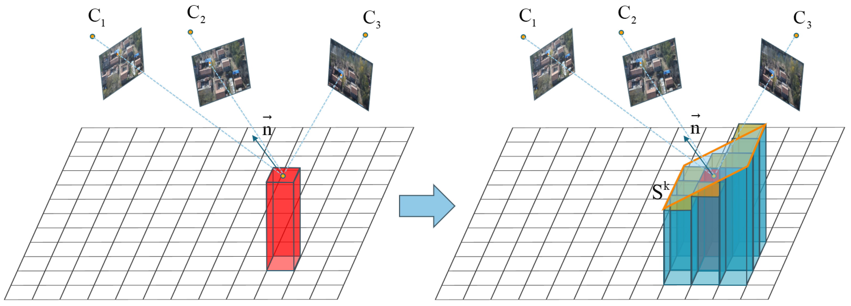
The core of digital orthophoto generation lies in obtaining the elevation and texture information of objects within the spatial scene. In order to obtain the elevation and texture of the spatial objects’s surface, as shown in Figure 1, the traditional method of generating digital orthophoto mainly draws inspiration from the concept of MVS. It involves reprojecting three-dimensional objects onto different images using the camera’s intrinsic and extrinsic parameters. By extracting two image patches centered around the reprojection point, this method then infers the likelihood of the object being at the current elevation based on a quantitative assessment of the similarity between these scenes. Consequently, it reconstructs the necessary spatial structural information of the scene, and the final results are obtained through top-view projection. We define such algorithms that utilize traditional geometry-based approaches to acquire explicit three-dimensional spatial structures and subsequently generate digital orthophotos as explicit methods. The generation process of many types of commercial software, such as Pix4D (version 2.0.104), is carried out using explicit methods. For example, Liu et al. [1] proposed a post-processing method based on Pix4D for digital orthophoto generation. Some works [2,3,4] are optimized for linear structures in structured scenes.

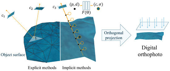
Figure 1. We categorize digital orthophoto generation methods into two types: explicit methods and implicit methods. The typical workflow of explicit methods involves obtaining the geometric structure with explicit parameters like mesh. The implicit methods are based on neural rendering, approximating the geometric structure with implicit neural networks. Both of them generate digital orthophoto through orthogonal projection.

As a rapidly advancing emerging neural rendering method, NeRF [5] has gained significant attention and shown great potential in recent years. NeRF-related methods inherently offer arbitrary viewpoints, theoretically making them applicable for digital orthophoto generation. They can be used in any scene as long as sparse reconstruction is completed. Therefore, we specifically focused on the feasibility of NeRF in digital orthophoto generation. As shown in Figure 1, NeRF initiates the rendering process by sampling a series of points along targeted rays (represented by the black dots), then estimates the volume density and radiance at specific viewpoints (represented by the circles with an orange outline) for these sample points with neural networks $F\left(\mathrm{\Theta }\right)$; finally, it applies volume rendering to produce the pixel values. As a specific viewpoint of the scene, the digital orthophoto can be rendered using NeRF by employing a set of parallel rays that are orthogonal to the ground. In this paper, we define the digital orthophoto generation methods based on neural rendering, which do not rely on traditional three-dimensional reconstruction, as implicit methods.

In this paper, we will compare the algorithmic processes and performance of explicit and implicit methods in digital orthophoto generation. Within the explicit methods, we selected the TDM algorithm [6], known for its exceptional speed performance. To unleash its potential, we conducted CUDA version porting and optimization modifications, significantly enhancing the generation efficiency. For implicit methods, we implemented orthographic view rendering based on NeRF and selected the speed-optimized Instant NGP [7] as a representative experiment. The experimental results reveal that the explicit method demonstrates notably high efficiency in generation speed. Both explicit and implicit methods yield acceptable levels of measurement accuracy and exhibit comparable rendering quality.

2. Related Work

2.1. DigitalOrthophoto Generation Methods

In digital photogrammetry, a mature workflow of digital orthophoto generation is presented in [8]. A general digital orthophoto generation approach often relies on 3D reconstruction. Schonberger et al. [9] proposed a complete structure-from-motion (SfM) pipeline. Shen et al. [10] proposed a patch-based dense reconstruction method, allowing for the integration with the SfM pipeline to achieve an entire 3D reconstruction process. Some works [11,12] used smartphone sensors to generate the 3D models. After the 3D reconstruction is completed, it can be orthogonally projected onto a horizontal plane to obtain the digital orthophoto. A digital orthophoto generation method with the assistance of Pix4D is proposed in [1]; they also propose post-processing methods based on Pix4D for digital orthophoto generation. Many efforts are being made to accelerate digital orthophoto generation, but these works are usually focused on specific scenarios. Some works have optimized digital orthophoto generation in structured scenes. For instance, Wang et al. [4] extracted and matched lines from the original images and then transformed these matched lines into the 3D model, reducing the computational cost of pixel-by-pixel matching in dense reconstruction. Li et al. [13] used deep learning methods to obtain a topological graph in the scenes, enhancing the accuracy at the edges of buildings. Lin et al. [2] arranged ground control points at the edges of buildings to ensure the accuracy of these edges. Some studies have made improvements for more specialized scenes. For instance, Lin et al. [14] focused on agricultural surveying scenarios, utilizing the spectral characteristics of vegetation to determine its location, thereby achieving fast digital orthophoto generation in agricultural mapping contexts. Zhao et al. [15] assumed the target scene to be a plane, employing simultaneous localization and mapping (SLAM) for real-time camera pose estimation and projecting the original images onto the imaging plane of the digital orthophoto. These methods speed up the digital orthophoto generation by sacrificing the generality of the algorithms. Some methods [16,17] utilize Digital Elevation Model (DEM) to accelerate the digital orthophoto generation, but this approach is constrained by the acquisition speed of the DEM.

Zhao et al. [6] were the first to propose a process for digital orthophoto generation directly using sparse point clouds. This approach eliminates the redundant computations that occur in the dense reconstruction phase of the standard 3D reconstruction-based digital orthophoto generation methods, significantly increasing the speed of generation.

2.2. NeRF with Sparse Parametric Encodings

In recent years, methods for novel view image synthesis on neural rendering have rapidly evolved. Mildenhall et al. [5] introduced NeRF, which represents a scene as a continuous neural radiance field. NeRF optimizes a fully connected deep network as an implicit function to approximate the volume density and view-dependent emitted radiance from 5D coordinates $(x,y,z,\theta ,\varphi )$, with $\sigma$ representing the volume density at a spatial point. To render an image from a specific novel viewpoint, NeRF initially (1) generates camera rays traversing the scene and samples a set of 3D points along these rays, (2) inputs the sampled points and viewing directions into the neural network to obtain a collection of densities RGB values, and (3) employs differentiable volume rendering to synthesize a 2D image.

Many recent works have incorporated sparse parametric encoding into NeRF for enhancement, generally aiming to pre-construct a series of auxiliary data structures with encoded features within the scene. We summarize these NeRFs with sparse parametric encoding into four stages in Figure 2: (1) scene representation, (2) radiance prediction, (3) differentiable renderer, and (4) loss function. For the first stage in Figure 2a, numerous sparse parametric encoding techniques have been proposed, such as dense and multi-resolution grids [7,18,19], plannar factorization [20,21,22], point clouds [23], and other formats [24,25]. The central concept behind these methods is to decouple local features of the scene from the MLP, thereby enabling the use of more flexible network architectures. They are typically represented by a grid, as shown in Figure 2a, resulting in the local encoding feature lookup table shown in the orange part. For the second stage in Figure 2b, a coarse–fine strategy is often used to sample along rays, and a cascaded MLP is typically used to predict volume density and view-dependent emitted radiance. Several studies have attempted to enhance rendering quality by improving sampling methods [22,26,27]; some have employed occupancy grids to achieve sampling acceleration [28]; others have focused on adjusting the MLP structure to facilitate easier network training [29]. For the third stage in Figure 2c, the figure exemplifies the most commonly used volume rendering, but other differentiable rendering methods are also employed [30], with Nvdiffrast [31] providing efficient implementations of various differentiable renderers. For the fourth stage in Figure 2d, the figure presents the most commonly used mean squared error loss between rendered and ground truth images, with some works introducing additional supervision, such as methods incorporating depth supervision [32,33]. With different scene representations, various loss functions are incorporated to constrain the network. Neural radiance fields can achieve photorealistic rendering quality and lighting effects, but it often takes hours to optimize the network parameters, and the training process is computationally expensive.

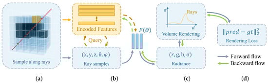
Figure 2. A schematic representation of NeRF with sparse parametric encoding. The process is divided into four stages: (a) scene representation, primarily defining auxiliary data structures for a scene’s sparse parametric encoding; (b) radiance prediction, where queried encoded features (orange arrows) and embedded sampling points are represented as feature embeddings and the radiance at these points is obtained through the function $F\left(\mathrm{\Theta }\right)$; (c) differentiable rendering, rendering meaningful pixel RGB values based on the radiance of sampling points; (d) loss computation, calculating the loss based on the rendering results, followed by backpropagation (green arrows) to optimize network parameters.

Both explicit and implicit methods require the initial step of SfM to obtain sparse point clouds and camera poses. The former predicts depth using multi-view geometry theories and describes the geometric structure of the scene using explicit parameters such as mesh, voxel, raster, etc. In contrast, implicit methods gradually fit to the real scene through implicit neural representation during the training process. Finally, both methods render digital orthophoto images from an orthographic viewpoint.

3. Method

An explicit digital orthophoto generation method typically involves the SfM and MVS processes. The TDM method facilitates the fast generation of digital orthophotos directly from sparse point clouds. Unlike MVS, the computation process of TDM is specifically tailored toward the final output of digital orthophotos. Factors unrelated to digital orthophotos are not involved in the computation, facilitating faster generation of digital orthophotos. So we selected the TDM algorithm as the representative explicit method for fast digital orthophoto generation and Instant NGP as the representative implicit method.

An implicit digital orthophoto generation method typically involves optimizing a group of parameters with posed images. This optimization process often takes several hours or even dozens of hours. Instant NGP [7] represents a speed-optimized neural radiance field, achieving the shortest optimization time among current radiance field methodologies. Hence, we select Instant NGP as the representative implicit method for fast digital orthophoto generation.

Both methods rely on the sparse reconstruction results from SfM. To generate digital orthophotos, both methods require prior information of accurate ground normal vectors. By using the Differential Global Positioning System (DGPS) information as a prior for sparse reconstruction, we can obtain accurate ground normal vectors while also recovering the correct scale of the scene.

3.1. Explicit Method—TDM

The TDM algorithm, when generating digital orthophotos, essentially processes information for each pixel, equivalent to raster data processing. To achieve the final rendering, the key lies in accurately estimating the elevation values and corresponding textures for each raster. The following will introduce the algorithm flow of our CUDA-adapted and optimized version of the TDM algorithm in this paper.

Raster Attribute Initialization: by specifying the spatial resolution $R_s$, the raster image G to be generated is obtained with dimensions $W\times H$, where each raster represents a pixel in the final digital orthophoto image. Each raster unit possesses five attributes: (1) raster color $C_o=({R^i}_g,{G^i}_g,{B^i}_g)$; (2) raster elevation $Z_g$; (3) raster normal vector $\overrightarrow{n}=(n_x,n_y,n_z)$. (4) Confidence score of raster elevation $S_g$. (5) The camera group to which the raster belongs $C_g$. As shown in Figure 3, the algorithm traverses through all three-dimensional point clouds and performs orthographic projection to obtain the raster unit $g^i$ corresponding to a certain three-dimensional point ${(X_i,Y_i,Z_i)}^T$. Subsequently, the elevation $Z_g$ of that raster is initialized.

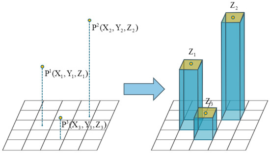
Figure 3. The figure illustrates the process of raster elevation initialization. In the initial stage, there are some points in three-dimensional space. Following the initialization process, rectangular raster units are obtained. The height of the vertical column represents the elevation values of each cell.

Then, we will search for the corresponding camera group $C_g$ for each raster containing an elevation value. This camera group retains the best-angle cameras in all eight directions that can see this raster, facilitating the subsequent process of finding and determining the views. As shown in Figure 4, the space is first evenly divided into eight regions. Then, the camera with the highest view score $S_v$ in each of the eight directions that can see the raster $g^i$ is retained.

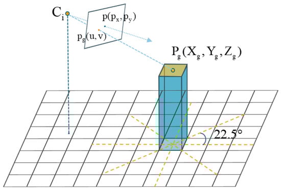
Figure 4. The figure illustrates the process of initializing the camera group. Based on the projection relationship of the pinhole camera, the projection $p_g$ of the raster’s world center point $P_g$ on the image plane is obtained. The original space is evenly divided into eight regions, and the camera with the highest $S_v$ in each region is found to be the camera group for this raster.

We denote the principal point coordinates of the image as ${(p_x,p_y)}^T$, and the world coordinates $P_g$ of the raster $g^i$, after being projected by the camera, as $p_g$. The optimal view score $S_v$ is then calculated as

$$S_v=\frac{1}{{(u-p_x)}^2+{(v-p_y)}^2+\epsilon }$$

(1)

Finally, the eight cameras with the highest scores in each direction are selected as a camera group for the raster. The camera with the highest score is considered as the optimal view camera $C_b$ for the raster unit.

Elevation Propagation: Given rasters with known elevation are considered as seed units $g_s$, and the propagation starts iteratively from these seed units. Each iteration propagates the elevation information Z from the seed raster unit to all raster units within a patch. Subsequently, the adjustment of $Z_g$ occurs via the random initialization of the normal vector $\overrightarrow{n}$, as shown in Figure 5. We project the i-th raster of the raster support plane $S^k$ onto a corresponding image $I^j$ in the camera group ${C_g}^i$, and the corresponding pixel color is denoted as $(R^{jki},G^{jki},B^{jki})$. The average color of the nine raster units projected onto the image $I^j$ in the raster support plane $S^k$ is denoted as $(\overline{R^{jk}},\overline{G^{jk}},\overline{B^{jk}})$. Define a color vector ${\mathbf{V}}^{jk}$ to represent the color information of $S^k$:

$${\mathbf{V}}^{jk}={(R^{jk1}-\overline{R^{jk}},G^{jk1}-\overline{G^{jk}},B^{jk1}-\overline{B^{jk}},\dots ,R^{jk9}-\overline{R^{jk}},G^{jk9}-\overline{G^{jk}},B^{jk9}-\overline{B^{jk}})}^T$$

(2)

Figure 5. The figure demonstrates the elevation propagation process. The red rectangular raster represents the seed unit. The seed unit with a known elevation and the surrounding eight raster units with unknown elevation form a raster support plane. The raster support plane calculates a matching score based on color consistency. If the score meets the threshold, the elevations of other raster units will be initialized based on the normal vector of the seed raster unit.

The number of cameras in the camera group of the i-th raster unit is denoted as ${N^i}_C$, and the number of color vectors that $S^k$ possesses is ${N^k}_C$. Therefore, the equation ${N^k}_C={\displaystyle \sum _{i=1}^9}{N^i}_C$ can be derived. The color vector corresponding to the optimal view camera $C_{bs}$ of the seed raster is taken as the reference vector. To measure the consistency of ${N^k}_C$ color vectors, the average cosine distance between the reference vector and other vectors is defined as the matching score ${M^k}_s$ for $S^k$:

$${M^k}_s=\frac{{\displaystyle \sum _{j=1\dots {N^k}_C,j\ne s,j\notin {{\mathrm{\Phi }}^k}_o}}\frac{{{\mathbf{V}}^{jk}}^T{\mathbf{V}}^{sk}}{∥{\mathbf{V}}^{jk}∥∥{\mathbf{V}}^{sk}∥}}{{N^k}_C-{N^k}_o}$$

(3)

where $\frac{{{\mathbf{V}}^{jk}}^T{\mathbf{V}}^{sk}}{∥{\mathbf{V}}^{jk}∥∥{\mathbf{V}}^{sk}∥}$ represents the cosine distance, ${\mathbf{V}}^{sk}$ is the reference vector, ${{\mathrm{\Phi }}^k}_o$ is the set of occluded images, and ${N^k}_o$ is the number of images in ${{\mathrm{\Phi }}^k}_o$.

Furthermore, we can evaluate the reasonableness of depth information through color consistency. Once the computed ${M^k}_s$ exceeds the confidence threshold $\eta$, the current depth information is considered reasonable. Then, we update the $Z_g$, $S_g$ and $\overrightarrow{n}$ of all raster units within the patch. During an iteration, there will be multiple random initializations of $\overrightarrow{n}$. If the matching score remains below $\eta$, elevation information will not be propagated.

Multi-resolution Interpolation-based Elevation Filling: The original algorithm gradually reduces $\eta$ after each iteration until the elevation propagation is complete. This will result in subsequently obtaining a lower confidence score for $Z_g$ and wasting a considerable amount of time. To efficiently reduce iteration time, we propose a multi-resolution interpolation-based elevation filling algorithm to acquire elevations of raster units with low confidence scores. When the initial value of $\eta$ is ${\eta }_0$, it gradually decreases with the increase in iteration count until it equals ${\eta }_e$. At this stage, we utilize the proposed algorithm to assign values to raster units $g^i$ without elevations, as shown in Figure 6.

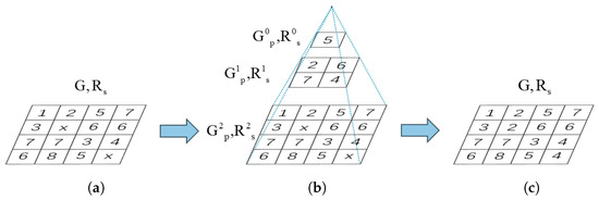
Figure 6. The figures illustrate the multi-resolution interpolation-based elevation filling process. (a) The raster image obtained after elevation propagation contains raster units with unknown elevations. (b) The process of generating the multi-resolution interpolation raster images. (c) The resulting raster image after elevation filling using the multi-resolution interpolation raster images.

After the elevation propagation, the initial seed ${g^i}_s$ for this filling algorithm is derived from raster units $g^i$ within the raster image G, where the confidence measure $S_g$ exceeds ${\eta }_0$. The spatial resolution ${R^i}_{sp}$ of the filling raster image ${G^i}_p$ for the i-th layer of this multi-resolution raster is as follows:

$${R^i}_{sp}=\frac{min[(X_{max}-X_{min}),(Y_{max}-Y_{min})]}{2^i}$$

(4)

where $X_{max}$ and $Y_{max}$ are the maximum values of the X- and Y-coordinates in this area. Likewise, $X_{min}$ and $Y_{min}$ are the minimum values. When multiple ${g^i}_s$ fall into the same raster unit $g^i$ of ${G^i}_p$, we set the average of these points as the elevation value for that raster unit. If no points fall within a specific raster unit, we will retrieve the elevation value corresponding to the raster position from multi-resolution interpolation raster image ${G^{i-1}}_p$ and set it as the elevation value for $g^i$. If ${R^i}_{sp}<R_s$, the process is repeated, continuously constructing ${G^i}_p$ as described above. Eventually, there are some raster units that have not been assigned elevation values in G. We will then search for the elevation values corresponding to the raster positions in the highest resolution interpolation raster image ${G^f}_p$ and assign them accordingly.

Texture Mapping: In each image, certain objects might be occluded by other objects, leading to erroneous texture mappings. Occlusion detection is necessary in such cases.

Subsequently, texture mapping is performed based on $g^i$ and the corresponding projection relationship with the optimal view camera $C_b$, obtaining color information $C_o=({R^i}_g,{G^i}_g,{B^i}_g)$ for the raster unit. Finally, the generation of the final digital orthophoto is completed.

3.2. Implicit Method—Instant NGP

We will use the most representative Instant NGP [7] as an example to illustrate the process of digital orthophoto generation using implicit methods. As a neural radiance field utilizing sparse parametric encodings, Instant NGP introduces multi-resolution hash encoding to address the $O\left(N^3\right)$ parameter complexity associated with dense voxel grids; Figure 7 illustrates this multiresolution hash encoding process in 2D.

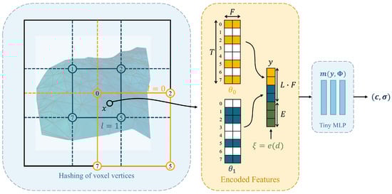
Figure 7. Illustration of the multiresolution hash encoding in 2D. For a given coordinate x, the method queries the encoded features on the surrounding voxels’ vertices (blue and orange circles) with the hashing result (numbers in the circles) and performs interpolation on the encoded features in ${\theta }_l$ across L levels. For a given direction d, the embedding function $e\left(d\right)$ is applied to generate auxiliary inputs $\mathrm{\xi }$. Subsequently, the encoded features at each level and auxiliary inputs will be concatenated as the final MLP embedding input $y\in {\mathbb{R}}^{LF+E}$ to obtain the radiance $(c,\sigma )$. Its optimizable parameters consist of L hash tables ${\theta }_l$ and tiny MLP $m(y;\mathrm{\Phi })$.

In practice, Instant NGP divides the scene into voxel grids with L levels of resolution. For each level of the resolution grids, a compact spatial hash table ${\theta }_l$ of a fixed size T is used to store the F-dimensional feature vectors on that resolution level’s grid. When querying the feature vector of a spatial coordinate x in Instant NGP, the process first identifies grid corners spatially close to x on each resolution layer. Then, the feature vectors of adjacent grid corners are looked up in ${\theta }_l$. Next, linear interpolation is performed to obtain the feature vector of the spatial coordinate x at that resolution level. This process is executed across all L resolution levels. Subsequently, these feature vectors from different resolution layers are concatenated with auxiliary inputs $\mathrm{\xi }\in {\mathbb{R}}^E$, forming the final MLP embedding input $y\in {\mathbb{R}}^{LF+E}$. Finally, Instant NGP uses a Tiny MLP $m(y;\mathrm{\Phi })$ to obtain the radiance $(c,\sigma )$ for the spatial coordinate x. This process also aligns with the generalized description of neural radiance fields based on sparse parametric encoding, as shown in Figure 2. Instant NGP can achieve a balance between performance, storage, and efficiency by selecting appropriate hash table sizes T.

As mentioned in Section 1, digital orthophotos can be rendered with neural approaches. In contrast to the typical pinhole camera imaging model, digital orthophotos are rendered using a set of parallel light rays perpendicular to the ground, as shown in Figure 1. To ensure that Instant NGP achieves a rendering quality comparable to explicit methods in scalable scenes, we adopted the largest scale model recommended in the paper.

4. Experiments and Analysis

The data utilized in this study were acquired from the Unmanned Aerial Vehicle (UAV) following a serpentine flight path pattern. A CW-25 Long Endurance Hybrid Gasoline & Battery VTOL drone was used in this data collection. It has a long service life, is fast, has a large payload, and is structurally stable and reliable. It is equipped with the RIY-DG4Pros five-lens camera, providing 42 million pixels and a resolution of 7952 × 5304 pixels. We established the drone ground station GCS1000. The UAV is equipped with the Novatel617D dual-antenna satellite positioning differential board card on board. Subsequently, through DGPS, the UAV can accurately capture changes in the ground station’s position, speed, and heading in real time.

We selected the TDM algorithm as the representative explicit method for digital orthophoto generation. Similarly, we used Instant NGP as the representative implicit method for digital orthophoto generation. The commercial software Pix4D is widely used and performs exceptionally well in digital orthophoto generation. Therefore, we have chosen its generated results as the benchmark for measuring accuracy. Pix4D, being an explicit method, requires the full process of traditional 3D reconstruction during digital orthophoto generation. Hence, for the time comparison test, we selected the TDM algorithm, which eliminates redundant computations during the dense reconstruction.

As described in this section, we initially conducted digital orthophoto generation tests on three common scenes: buildings, roads, and rivers. The objective was to demonstrate the image generation quality and algorithm robustness of both explicit and implicit methods across various scenes. Subsequently, to assess the accuracy of the two methods, comparisons were made with the commercial software Pix4D regarding measurement precision. Finally, to evaluate the efficiency of both methods, we measured the time required for generating scenes of different sizes.

4.1. Test on Various Scenes

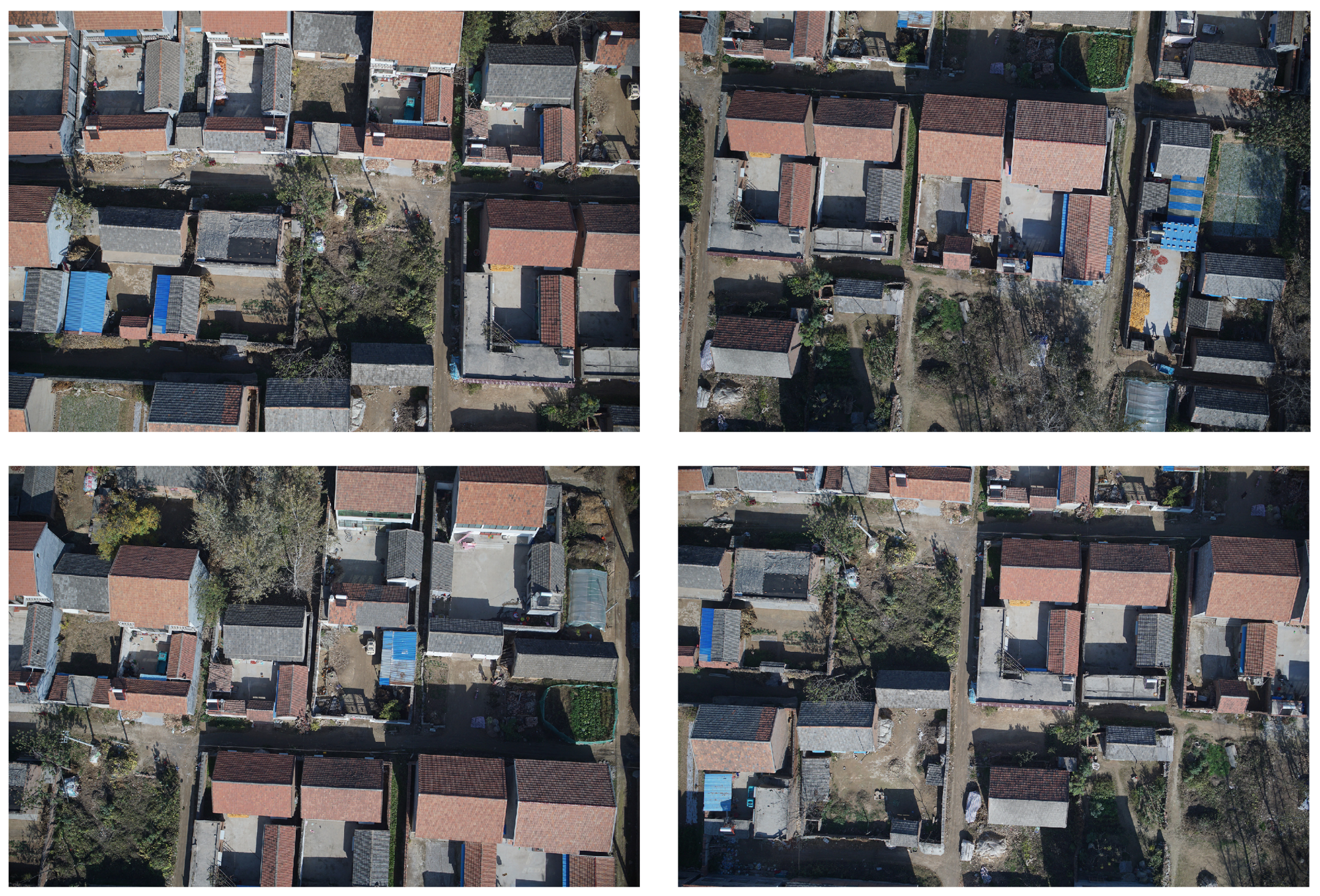
Figure 8 shows a set of original village photo data used for testing, including numerous scenes of slanted roofs of houses, trees, and other objects. We performed sparse reconstruction in conjunction with the camera’s DGPS information, enabling the recovery of accurate scale information and spatial relationships. The resultant 3D sparse point cloud, as shown in Figure 9, and camera poses served as prior information for subsequent explicit and implicit methods in digital orthophoto generation. The resulting digital orthophotos after the final processing through the explicit and implicit methods are shown in Figure 10.

Figure 8. The original images of some village scenes captured by unmanned aerial vehicles.

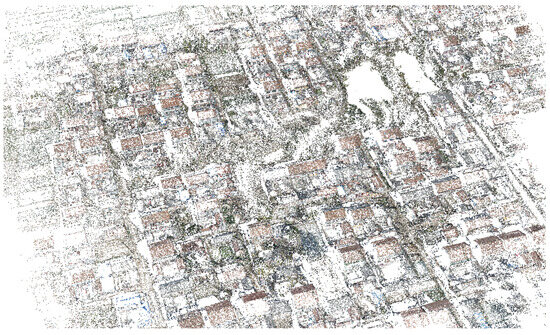
Figure 9. The point cloud of the village scenery obtained after sparse reconstruction.

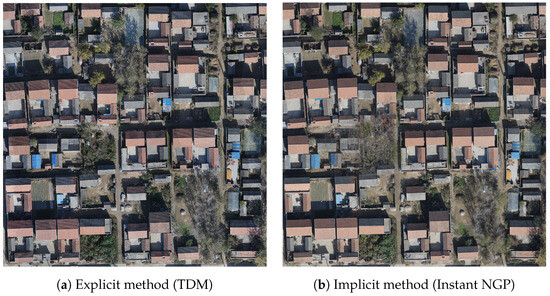
Figure 10. The figure illustrates the digital orthophoto generation results from two methods within the same village scene. (a) depicts the output derived from the explicit method. (b) depicts the output obtained from the implicit method.

As shown in Figure 11, we conducted digital orthophoto generation tests for various scenes using both explicit and implicit methods. Figure 11a,b show that TDM may lead to inaccuracies in areas experiencing sudden height variations, for example, the roof edges of houses, while Instant NGP can accurately depict sudden height variations. Figure 11c,d show that moving objects within the scene may induce ghostly artifacts in the results of Instant NGP but have a minimal impact on TDM. Figure 11e,f show that the clarity of the outputs of Instant NGP does not match that of TDM. The imaging quality of implicit methods is predominantly influenced by the model scale, whereas TDM is directly dictated by the clarity of the original image.

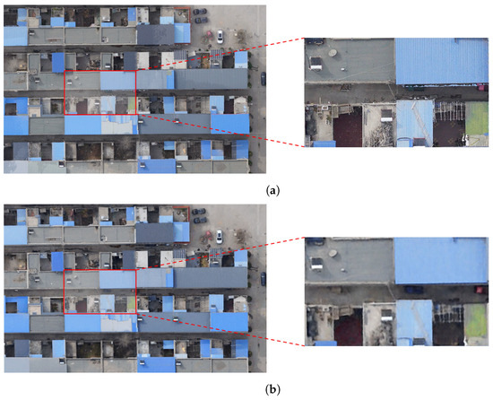
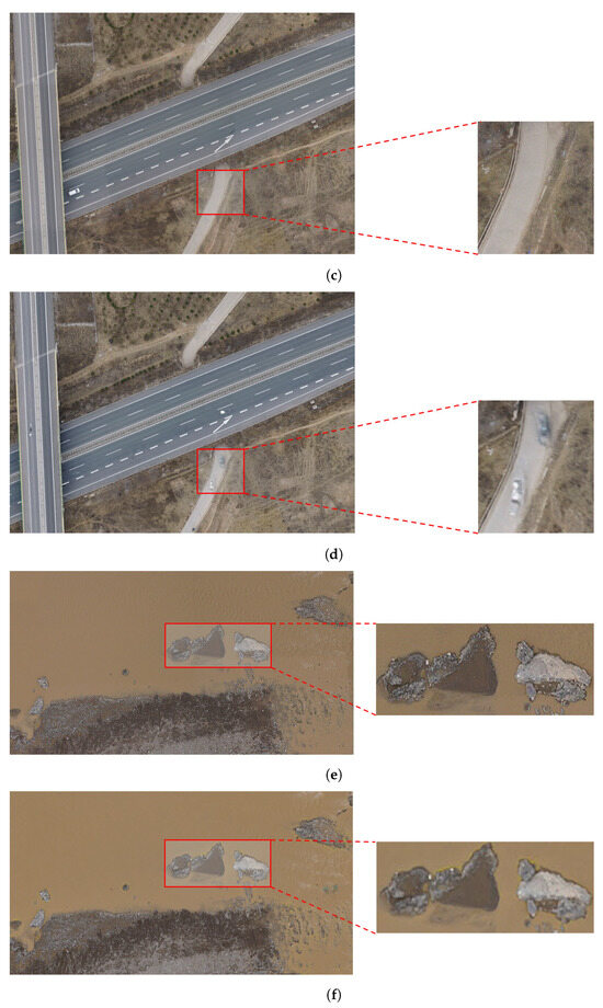
Figure 11. The figure shows digital orthophoto of scenes “houses”, “bridges”, and “rivers” generated using two different methods. Images (a,c,e) were generated using the explicit method (TDM), while images (b,d,f) are generated using the implicit method (Instant NGP).

To quantitatively analyze the quality of the digital orthophoto generated using the two methods, we employed two no-reference image quality assessment techniques, Brisque [34] and NIQE [35]. The results in Table 1 show that, in the majority of scenarios, the quality generated by the explicit method (TDM) surpasses that of the implicit method (Instant NGP).

Table 1. Quality assessment of images generated using two methods in different scenes and comparisons with the real image. The ↓ means lower is better.

Scenes Method|Metric	Houses		Bridges		River
	Brisque↓	NIQE↓	Brisque↓	NIQE↓	Brisque↓	NIQE↓
TDM (cuda)	12.96	2.77	7.88	2.33	12.90	5.01
Instant NGP	50.93	5.47	60.26	7.43	23.66	3.99
Real Images	6.72	1.67	5.91	1.72	7.74	1.74

Combining qualitative and quantitative analysis, it can be concluded that the TDM algorithm exhibits superior imaging clarity but demonstrates inaccuracies in areas experiencing sudden height variations. Conversely, Instant NGP is capable of capturing the majority of the scene’s structure accurately, yet its imaging clarity is constrained by the scale of the model and may produce ghostly artifacts. Both methods are capable of generating usable digital orthophoto.

4.2. Evaluation of Accuracy

An important characteristic of digital orthophotos is map geometric accuracy, so the accuracy of distance measurements is crucial. To validate the measurement accuracy of different digital orthophoto generation methods, we selected a specific area within the city for subsequent testing scenes. We utilized explicit methods (TDM), implicit methods (Instant NGP), and commercial software (Pix4D) to generate digital orthophoto, followed by comparing length measurements, as shown in Figure 12. The box plot displays the differences in distance measurements in digital orthophotos, as can be seen from Figure 13. The median of the box plot generated from Pix4D-to-TDM is 0.0376 m, while the other median from Pix4D-to-Instant NGP is 0.0442 m, both around 0.04 m. In comparison with Pix4D, this study concludes that both the explicit method (TDM) and the implicit method (Instant NGP) for digital orthophoto generation meet the requirements for mapping purposes.

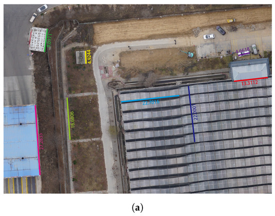
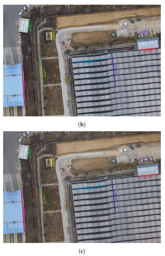
Figure 12. Digital orthophotos generated by TDM, Instant NGP and Pix4D.The segments with consistent colors and corresponding values represent identical distances measured across the three results. (a) Distance measurement of the explicit method (TDM), (b) Distance measurement of the implicit method (Instant NGP), (c) distance measurement of Pix4D.

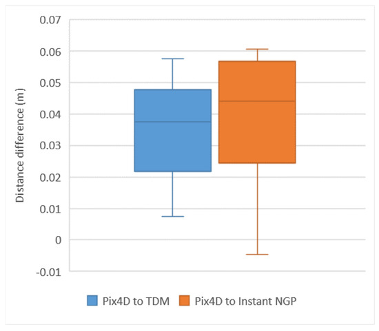
Figure 13. The box plot shows the differences in distance measurements between the explicit method (TDM) and the implicit method (Instant NGP) compared to Pix4D in the same scene, as depicted in Figure 12.

Furthermore, because the brightness of the color difference map can represent the degree of difference between digital orthophoto generated by different algorithms at the same location, in order to further measure the accuracy for digital orthophoto generation, this paper establishes the color difference maps between those methods. As shown in Figure 14, the color difference map shows that explicit methods (TDM) and implicit methods (Instant NGP) produced the same measurability and visibility of the generated digital orthophoto as those generated by the commercial software (Pix4D). In general, the accuracy of the two methods is acceptable according to the comparison with commercial software (Pix4D).

Figure 14. Color difference map between each of the two results. (a) Color difference map between Pix4D and TDM. (b) Color difference map between Pix4D and Instant NGP.

4.3. Evaluation of Efficiency

To verify the generation efficiency between explicit and implicit methods, in this section, we conducted tests on the generation time of digital orthophotos in five different size scenes. These two types of methods were run on a personal computer with an Intel (R) Core (TM) i7-12700 CPU @ 4.90 GHz and an NVIDIA GeForce RTX 3090.

Table 2 illustrates the time consumption for digital orthophoto generation using TDM and Instant NGP at different scene sizes. For TDM, the time measurement ranges from obtaining sparse reconstruction results to the generation of digital orthophotos. For Instant NGP, it starts from acquiring sparse reconstruction results, proceeds through model training, and culminates in rendering digital orthophoto. Across five different scene sizes, the TDM algorithm exhibits superior speed performance compared to Instant NGP, with its runtime reduced by two orders of magnitude. Therefore, the explicit method currently holds a significant advantage over the implicit method in terms of efficiency in digital orthophoto generation.

Table 2. Efficiency comparison of three methods of various scene sizes.

Scene Size (m) @Images	Method
	TDM	Instant NGP
$150\times 150$ @ 78	36 s	10,243 s
$200\times 200$ @ 130	60 s	16,931 s
$250\times 250$ @ 256	88 s	33,210 s
$300\times 250$ @ 281	103 s	36,454 s
$300\times 300$ @ 333	129 s	43,576 s

5. Conclusions

In this paper, we categorized the methods for digital orthophoto generation into explicit and implicit methods, exploring the potential of using NeRF for implicit digital orthophoto generation. We selected the most representative fast algorithms from the two categories: the TDM algorithm and Instant NGP. Additionally, we adapted and optimized TDM algorithm to a CUDA version, significantly enhancing the efficiency of digital orthophoto generation.

In both explicit and implicit methods, an initial step involves sparse reconstruction to obtain camera poses, point clouds, and other prior information. The former employs an elevation propagation process that explicitly integrates the local color consistency of images with multi-view geometry theories to acquire scene elevation information and corresponding textures. Conversely, in NeRF, the loss function is designed as the color difference between rendered and real images. Throughout the training process, the neural network gradually fits into the real scene, implicitly capturing the surfaces and textures of scene objects and synthesizing novel view images through differentiable rendering. Finally, both methods complete the entire process to generate digital orthophoto.

We conducted tests on explicit and implicit methods for digital orthophoto generation in various scenes, measuring the generation efficiency and result quality. We employed the commercial software Pix4D as a standard for assessing measurement accuracy and reliability, evaluating both methods. The results indicate that currently, explicit methods exhibit higher efficiency and lower computational resource requirements in generation compared to implicit methods, achieving results with respective advantages and disadvantages. Moreover, both methods meet the requirements for measurement accuracy. In our future work, we aim to further explore the development of implicit methods for digital orthophoto generation, accelerating the generation speed and enhancing the clarity of implicit methods by adding more constraints suitable for digital orthophoto generation.

References

- Liu, Y.; Zheng, X.; Ai, G.; Zhang, Y.; Zuo, Y. Generating a high-precision true digital orthophoto map based on UAV images. ISPRS Int. J. Geo-Inf. 2018, 7, 333. [Google Scholar] [CrossRef]
- Lin, T.Y.; Lin, H.L.; Hou, C.W. Research on the production of 3D image cadastral map. In Proceedings of the 2018 IEEE International Conference on Applied System Invention (ICASI), Tokyo, Japan, 13–17 April 2018; pp. 259–262. [Google Scholar]
- Barazzetti, L.; Brumana, R.; Oreni, D.; Previtali, M.; Roncoroni, F. True-orthophoto generation from UAV images: Implementation of a combined photogrammetric and computer vision approach. ISPRS Ann. Photogramm. Remote Sens. Spat. Inf. Sci. 2014, 2, 57–63. [Google Scholar] [CrossRef]
- Wang, Q.; Yan, L.; Sun, Y.; Cui, X.; Mortimer, H.; Li, Y. True orthophoto generation using line segment matches. Photogramm. Rec. 2018, 33, 113–130. [Google Scholar] [CrossRef]
- Mildenhall, B.; Srinivasan, P.P.; Tancik, M.; Barron, J.T.; Ramamoorthi, R.; Ng, R. Nerf: Representing scenes as neural radiance fields for view synthesis. Commun. ACM 2021, 65, 99–106. [Google Scholar] [CrossRef]
- Zhao, Z.; Jiang, G.; Li, Y. A Novel Method for Digital Orthophoto Generation from Top View Constrained Dense Matching. Remote Sens. 2022, 15, 177. [Google Scholar] [CrossRef]
- Müller, T.; Evans, A.; Schied, C.; Keller, A. Instant neural graphics primitives with a multiresolution hash encoding. ACM Trans. Graph. (ToG) 2022, 41, 1–15. [Google Scholar] [CrossRef]
- DeWitt, B.A.; Wolf, P.R. Elements of Photogrammetry (with Applications in GIS); McGraw-Hill Higher Education: New York, NY, USA, 2000. [Google Scholar]
- Schonberger, J.L.; Frahm, J.M. Structure-from-motion revisited. In Proceedings of the IEEE Conference on Computer Vision and Pattern Recognition, Las Vegas, NV, USA, 27–30 June 2016; pp. 4104–4113. [Google Scholar]
- Shen, S. Accurate multiple view 3D reconstruction using patch-based stereo for large-scale scenes. IEEE Trans. Image Process. 2013, 22, 1901–1914. [Google Scholar] [CrossRef]
- Fang, K.; Zhang, J.; Tang, H.; Hu, X.; Yuan, H.; Wang, X.; An, P.; Ding, B. A quick and low-cost smartphone photogrammetry method for obtaining 3D particle size and shape. Eng. Geol. 2023, 322, 107170. [Google Scholar] [CrossRef]
- Tavani, S.; Granado, P.; Riccardi, U.; Seers, T.; Corradetti, A. Terrestrial SfM-MVS photogrammetry from smartphone sensors. Geomorphology 2020, 367, 107318. [Google Scholar] [CrossRef]
- Li, Z.; Wegner, J.D.; Lucchi, A. Topological map extraction from overhead images. In Proceedings of the IEEE/CVF International Conference on Computer Vision, Seoul, Republic of Korea, 27 October–2 November 2019; pp. 1715–1724. [Google Scholar]
- Lin, Y.C.; Zhou, T.; Wang, T.; Crawford, M.; Habib, A. New orthophoto generation strategies from UAV and ground remote sensing platforms for high-throughput phenotyping. Remote Sens. 2021, 13, 860. [Google Scholar] [CrossRef]
- Zhao, Y.; Cheng, Y.; Zhang, X.; Xu, S.; Bu, S.; Jiang, H.; Han, P.; Li, K.; Wan, G. Real-time orthophoto mosaicing on mobile devices for sequential aerial images with low overlap. Remote Sens. 2020, 12, 3739. [Google Scholar] [CrossRef]
- Hood, J.; Ladner, L.; Champion, R. Image processing techniques for digital orthophotoquad production. Photogramm. Eng. Remote Sens. 1989, 55, 1323–1329. [Google Scholar]
- Fu, J. DOM generation from aerial images based on airborne position and orientation system. In Proceedings of the 2010 6th International Conference on Wireless Communications Networking and Mobile Computing (WiCOM), Chengdu, China, 23–25 September 2010; pp. 1–4. [Google Scholar]
- Sun, C.; Sun, M.; Chen, H.T. Direct voxel grid optimization: Super-fast convergence for radiance fields reconstruction. In Proceedings of the IEEE/CVF Conference on Computer Vision and Pattern Recognition, New Orleans, LA, USA, 18–24 June 2022; pp. 5459–5469. [Google Scholar]
- Fridovich-Keil, S.; Yu, A.; Tancik, M.; Chen, Q.; Recht, B.; Kanazawa, A. Plenoxels: Radiance fields without neural networks. In Proceedings of the IEEE/CVF Conference on Computer Vision and Pattern Recognition, New Orleans, LA, USA, 18–24 June 2022; pp. 5501–5510. [Google Scholar]
- Chen, A.; Xu, Z.; Geiger, A.; Yu, J.; Su, H. Tensorf: Tensorial radiance fields. In Proceedings of the European Conference on Computer Vision, Tel Aviv, Israel, 23–27 October 2022; Springer: Berlin/Heidelberg, Germany, 2022; pp. 333–350. [Google Scholar]
- Fridovich-Keil, S.; Meanti, G.; Warburg, F.R.; Recht, B.; Kanazawa, A. K-planes: Explicit radiance fields in space, time, and appearance. In Proceedings of the IEEE/CVF Conference on Computer Vision and Pattern Recognition, Vancouver, BC, Canada, 17–24 June 2023; pp. 12479–12488. [Google Scholar]
- Hu, W.; Wang, Y.; Ma, L.; Yang, B.; Gao, L.; Liu, X.; Ma, Y. Tri-miprf: Tri-mip representation for efficient anti-aliasing neural radiance fields. In Proceedings of the IEEE/CVF International Conference on Computer Vision, Paris, France, 2–3 October 2023; pp. 19774–19783. [Google Scholar]
- Xu, Q.; Xu, Z.; Philip, J.; Bi, S.; Shu, Z.; Sunkavalli, K.; Neumann, U. Point-nerf: Point-based neural radiance fields. In Proceedings of the IEEE/CVF Conference on Computer Vision and Pattern Recognition, New Orleans, LA, USA, 18–24 June 2022; pp. 5438–5448. [Google Scholar]
- Yu, A.; Li, R.; Tancik, M.; Li, H.; Ng, R.; Kanazawa, A. Plenoctrees for real-time rendering of neural radiance fields. In Proceedings of the IEEE/CVF International Conference on Computer Vision, Montreal, BC, Canada, 11–17 October 2021; pp. 5752–5761. [Google Scholar]
- Kulhanek, J.; Sattler, T. Tetra-NeRF: Representing Neural Radiance Fields Using Tetrahedra. arXiv 2023, arXiv:2304.09987. [Google Scholar]
- Barron, J.T.; Mildenhall, B.; Tancik, M.; Hedman, P.; Martin-Brualla, R.; Srinivasan, P.P. Mip-nerf: A multiscale representation for anti-aliasing neural radiance fields. In Proceedings of the IEEE/CVF International Conference on Computer Vision, Montreal, BC, Canada, 11–17 October 2021; pp. 5855–5864. [Google Scholar]
- Barron, J.T.; Mildenhall, B.; Verbin, D.; Srinivasan, P.P.; Hedman, P. Mip-nerf 360: Unbounded anti-aliased neural radiance fields. In Proceedings of the IEEE/CVF Conference on Computer Vision and Pattern Recognition, New Orleans, LA, USA, 18–24 June 2022; pp. 5470–5479. [Google Scholar]
- Li, R.; Tancik, M.; Kanazawa, A. Nerfacc: A general nerf acceleration toolbox. arXiv 2022, arXiv:2210.04847. [Google Scholar]
- Zhang, K.; Riegler, G.; Snavely, N.; Koltun, V. Nerf++: Analyzing and improving neural radiance fields. arXiv 2020, arXiv:2010.07492. [Google Scholar]
- Kerbl, B.; Kopanas, G.; Leimkühler, T.; Drettakis, G. 3D gaussian splatting for real-time radiance field rendering. ACM Trans. Graph. (ToG) 2023, 42, 1–14. [Google Scholar] [CrossRef]
- Laine, S.; Hellsten, J.; Karras, T.; Seol, Y.; Lehtinen, J.; Aila, T. Modular Primitives for High-Performance Differentiable Rendering. ACM Trans. Graph. 2020, 39, 1–14. [Google Scholar] [CrossRef]
- Roessle, B.; Barron, J.T.; Mildenhall, B.; Srinivasan, P.P.; Nießner, M. Dense depth priors for neural radiance fields from sparse input views. In Proceedings of the IEEE/CVF Conference on Computer Vision and Pattern Recognition, New Orleans, LA, USA, 18–24 June 2022; pp. 12892–12901. [Google Scholar]
- Deng, K.; Liu, A.; Zhu, J.Y.; Ramanan, D. Depth-supervised nerf: Fewer views and faster training for free. In Proceedings of the IEEE/CVF Conference on Computer Vision and Pattern Recognition, New Orleans, LA, USA, 18–24 June 2022; pp. 12882–12891. [Google Scholar]
- Mittal, A.; Moorthy, A.K.; Bovik, A.C. No-Reference Image Quality Assessment in the Spatial Domain. IEEE Trans. Image Process. 2012, 21, 4695–4708. [Google Scholar] [CrossRef]
- Mittal, A.; Soundararajan, R.; Bovik, A.C. Making a “Completely Blind” Image Quality Analyzer. IEEE Signal Process. Lett. 2013, 20, 209–212. [Google Scholar] [CrossRef]
Disclaimer/Publisher’s Note: The statements, opinions and data contained in all publications are solely those of the individual author(s) and contributor(s) and not of MDPI and/or the editor(s). MDPI and/or the editor(s) disclaim responsibility for any injury to people or property resulting from any ideas, methods, instructions or products referred to in the content. |
© 2024 by the authors. Licensee MDPI, Basel, Switzerland. This article is an open access article distributed under the terms and conditions of the Creative Commons Attribution (CC BY) license (https://creativecommons.org/licenses/by/4.0/).