


Accurate and Rapid Extraction of Aquatic Vegetation in the China Side of the Amur River Basin Based on Landsat Imagery


 ,
, 
Abstract
1. Introduction
2. Materials and Methods
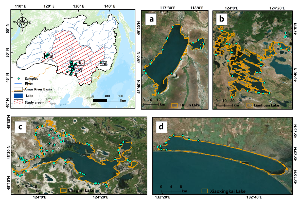
2.1. Study Area
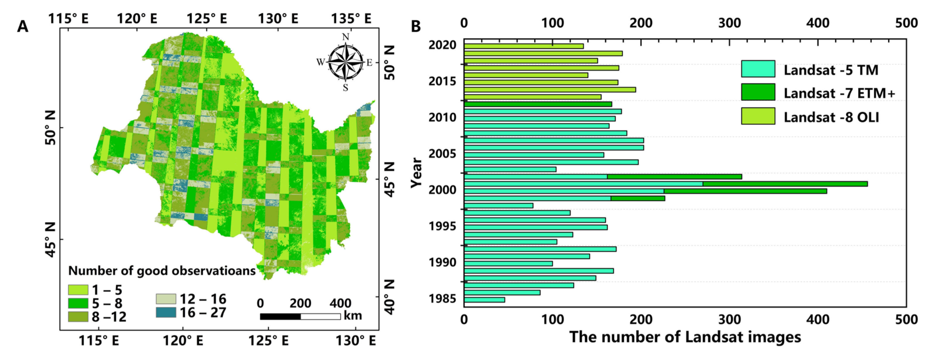
2.2. Remote Sensing Data
2.3. Ground Sample Data
2.4. Methodologies
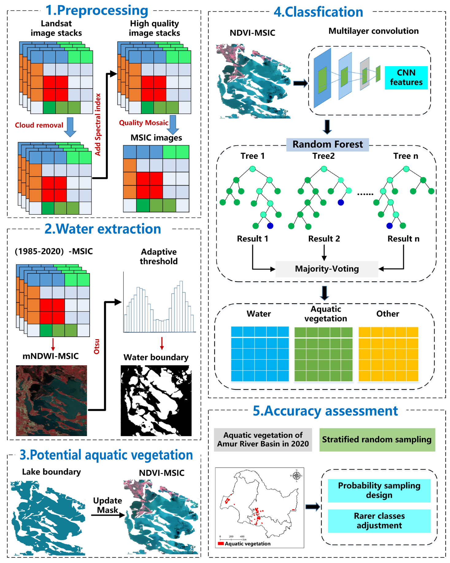
2.4.1. Basic Idea
2.4.2. The Maximum Spectral Index Composite (MSIC) and Otsu
2.4.3. Spectral Feature Construction
2.4.4. Delineating Spatial Extents of Lakes in the CARB
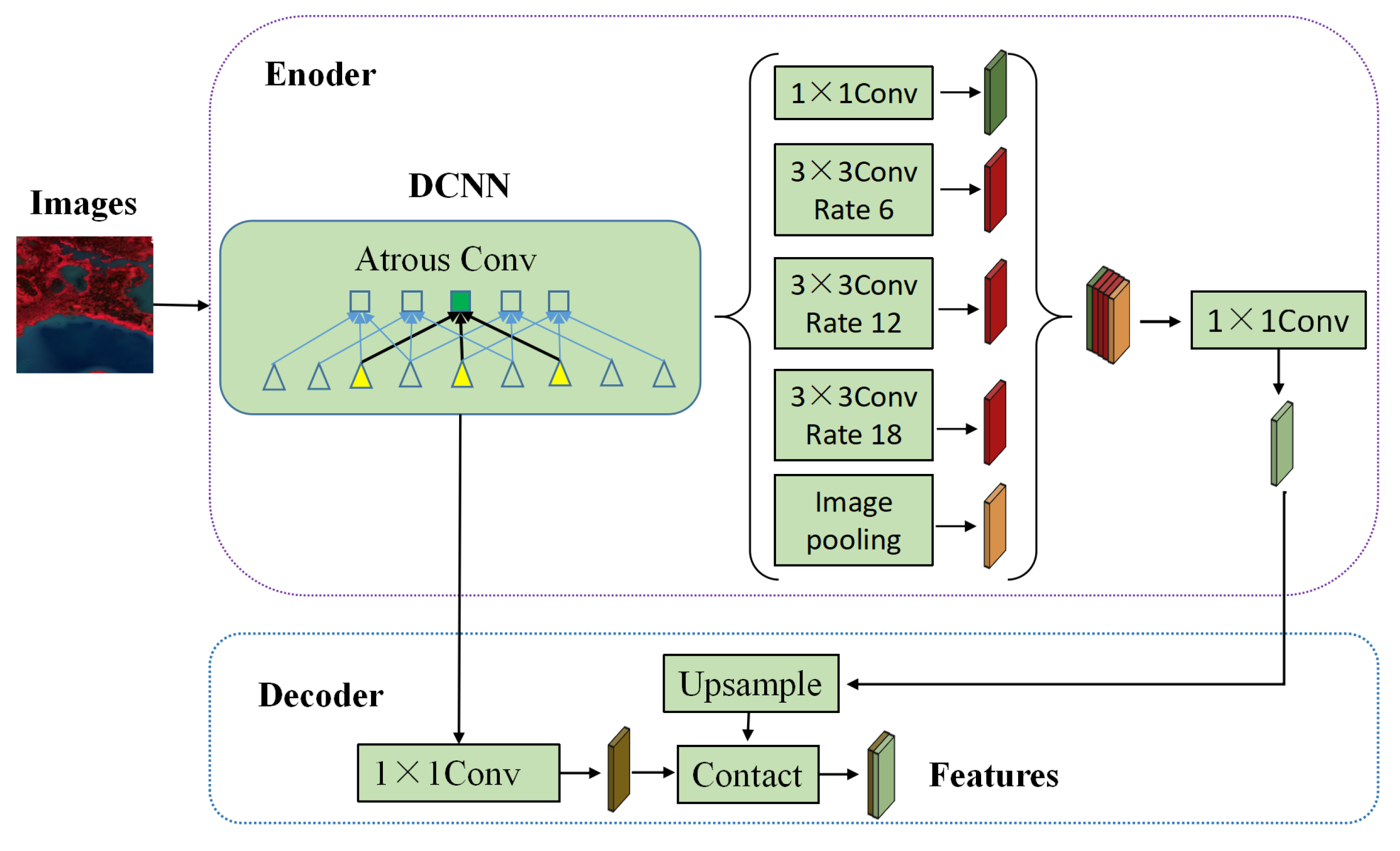
2.4.5. Convolutional Neural Network (CNN)
2.4.6. Random Forest (RF) Classification Algorithm
2.4.7. Accuracy Assessment
3. Results
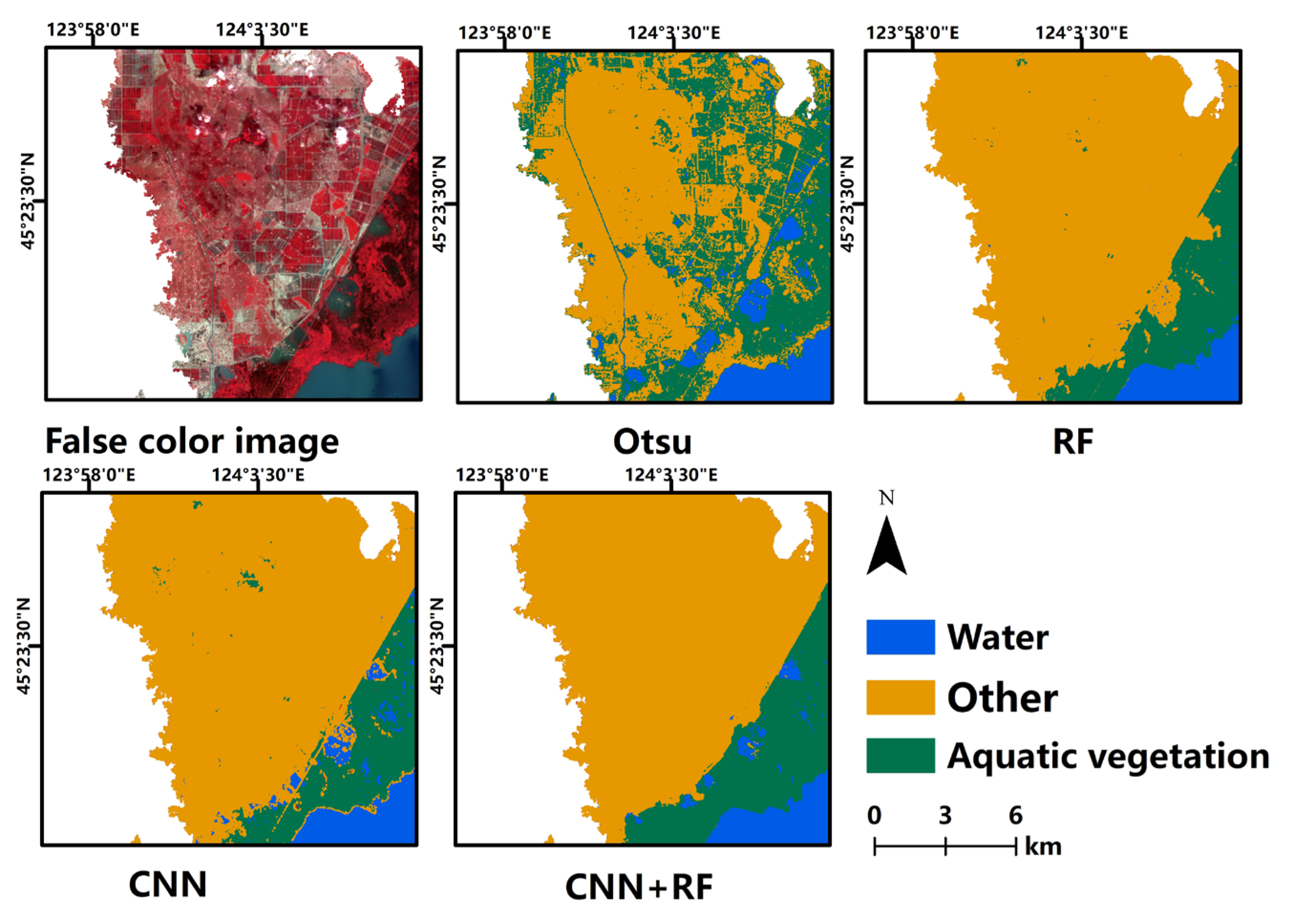
3.1. Accuracy Assessment
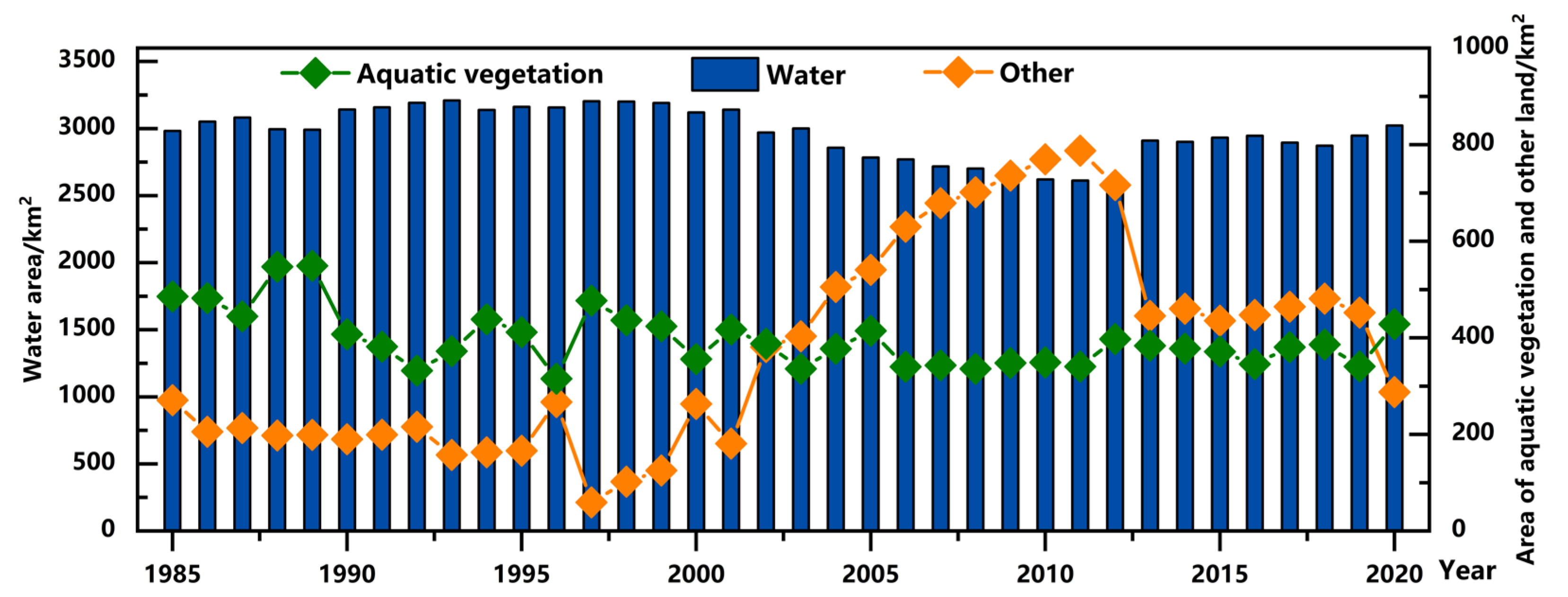
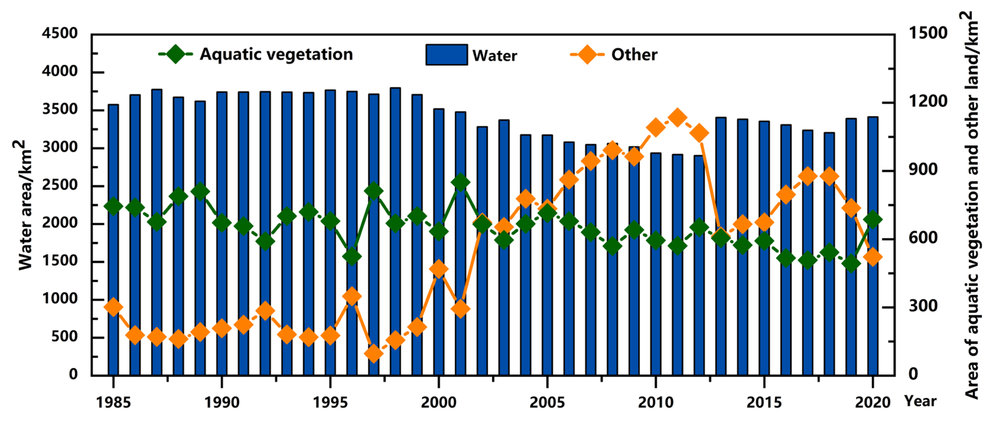
3.2. Analysis of the Spatial–Temporal Changes of the Overall Water and Aquatic Vegetation in the Study Area
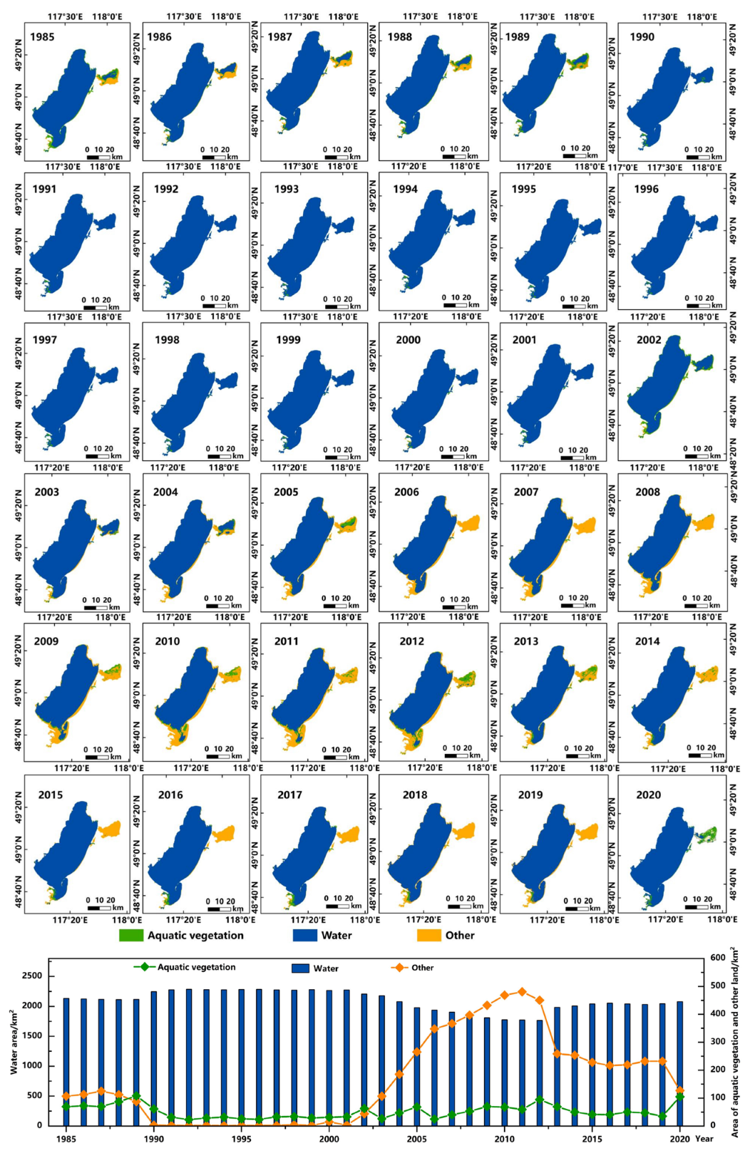
3.2.1. Temporal and Spatial Changes of Aquatic Vegetation in Hulun Lake
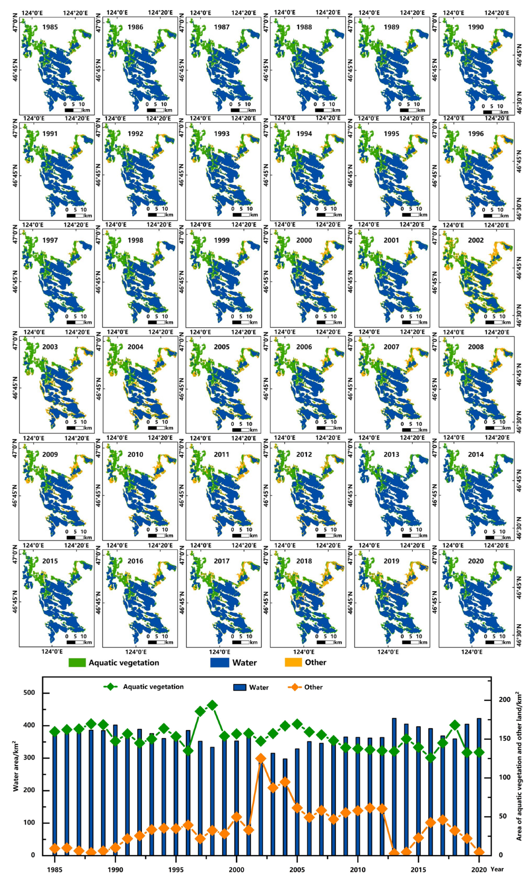
3.2.2. Temporal and Spatial Changes of Aquatic Vegetation in Lianhuan Lake
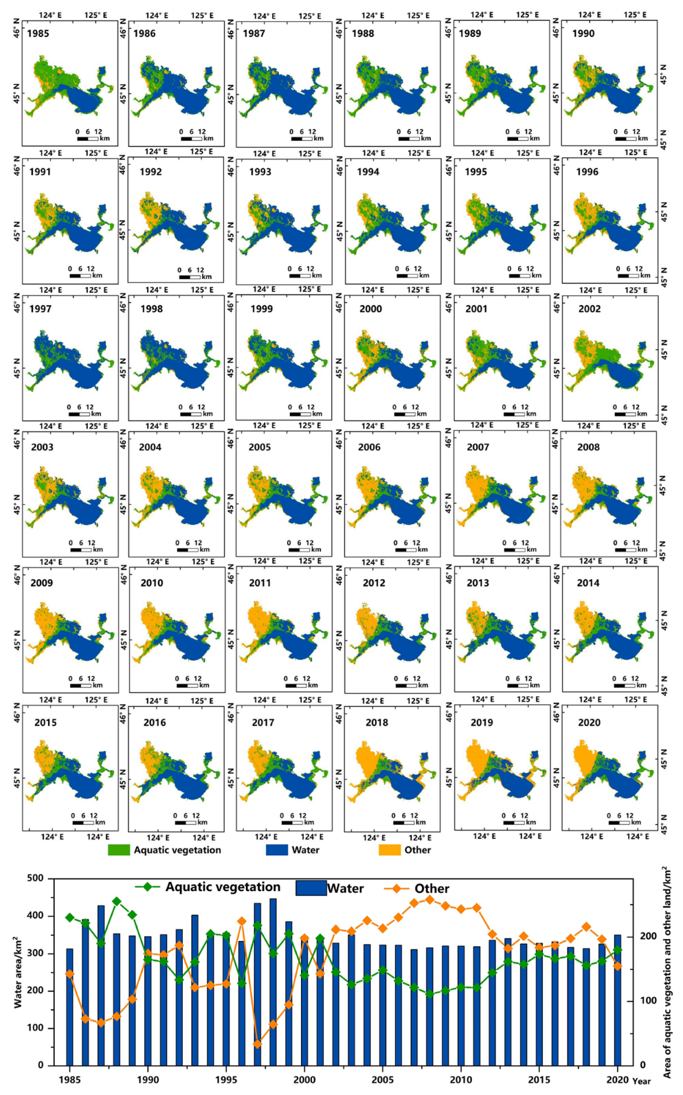
3.2.3. Temporal and Spatial Changes of Aquatic Vegetation in Chagan Lake
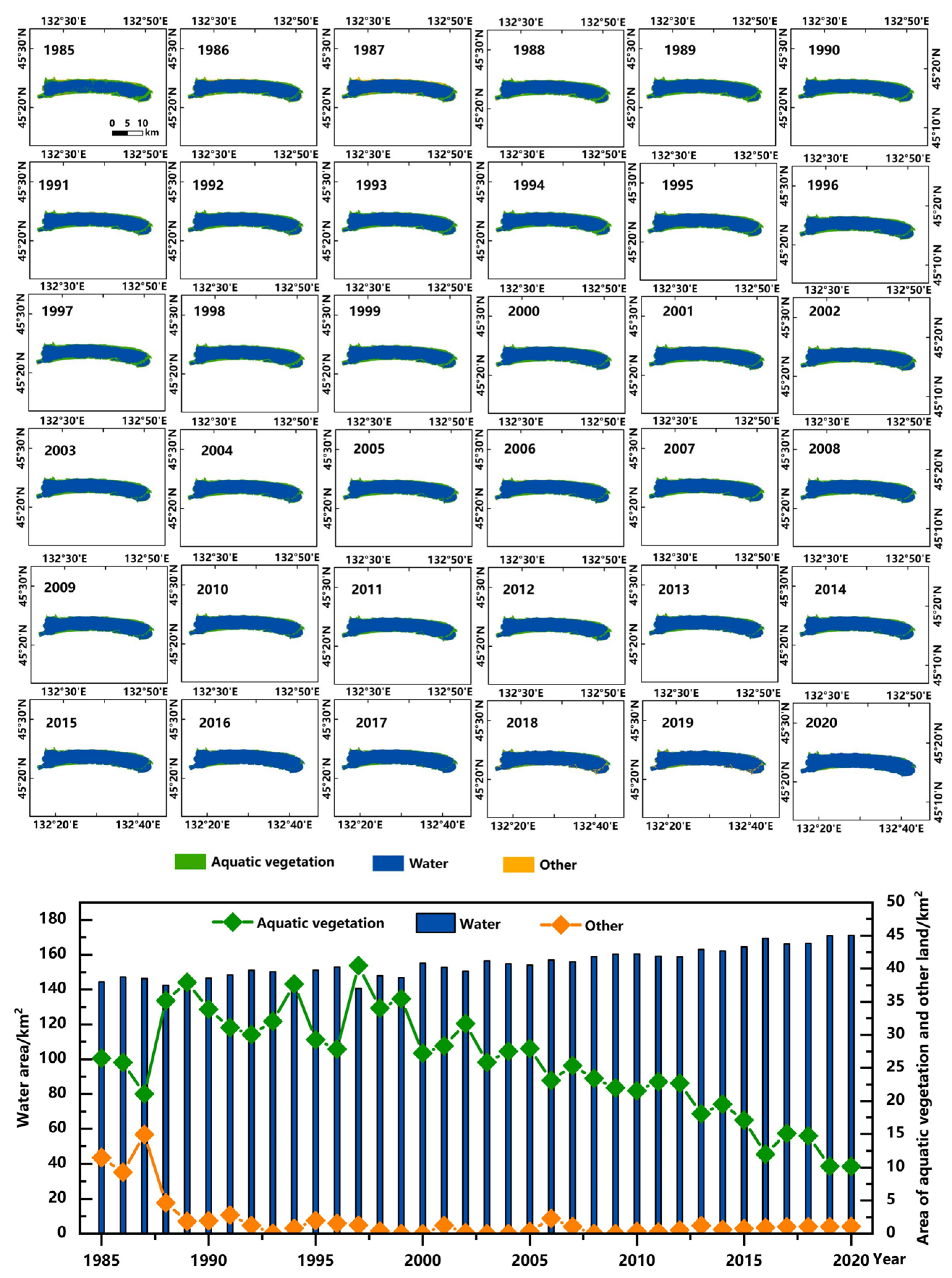
3.2.4. Temporal and Spatial Changes of Aquatic Vegetation in Xiaoxingkai Lake
4. Discussion
4.1. The Advantages of the Model in Large-Scale Extraction of Aquatic Vegetation
4.2. Uncertainties in Aquatic Vegetation Mapping
5. Conclusions
Author Contributions
Funding
Data Availability Statement
Acknowledgments
Conflicts of Interest
References
- Yang, G.; Ma, R.; Zhang, L.; Jiang, J.; Yao, S.; Zhang, M.; Zeng, H.D. Lake Status, Major Problems and Protection Strategy in China. J. Lake Sci. 2010, 22, 799–810. [Google Scholar]
- Parkes, M. Personal Commentaries on “Ecosystems and Human Well-Being: Health Synthesis—A Report of the Millennium Ecosystem Assessment”. EcoHealth 2006, 3, 136–140. [Google Scholar] [CrossRef]
- Inácio, M.; Barceló, D.; Zhao, W.; Pereira, P. Mapping Lake Ecosystem Services: A Systematic Review. Sci. Total Environ. 2022, 847, 157561. [Google Scholar] [CrossRef] [PubMed]
- Jeppesen, E.; Søndergaard, M.; Søndergaard, M.; Christoffersen, K. The Structuring Role of Submerged Macrophytes in Lakes; Springer Science & Business Media: Berlin/Heidelberg, Germany, 2012; Volume 131, ISBN 1-4612-0695-2. [Google Scholar]
- Horppila, J.; Nurminen, L. Effects of Submerged Macrophytes on Sediment Resuspension and Internal Phosphorus Loading in Lake Hiidenvesi (Southern Finland). Water Res. 2003, 37, 4468–4474. [Google Scholar] [CrossRef] [PubMed]
- Jia, M.; Mao, D.; Wang, Z.; Ren, C.; Zhu, Q.; Li, X.; Zhang, Y. Tracking Long-Term Floodplain Wetland Changes: A Case Study in the China Side of the Amur River Basin. Int. J. Appl. Earth Obs. Geoinf. 2020, 92, 102185. [Google Scholar] [CrossRef]
- Murphy, F.; Schmieder, K.; Baastrup-Spohr, L.; Pedersen, O.; Sand-Jensen, K. Five Decades of Dramatic Changes in Submerged Vegetation in Lake Constance. Aquat. Bot. 2018, 144, 31–37. [Google Scholar] [CrossRef]
- Zhang, Y.; Liu, X.; Qin, B.; Shi, K.; Deng, J.; Zhou, Y. Aquatic Vegetation in Response to Increased Eutrophication and Degraded Light Climate in Eastern Lake Taihu: Implications for Lake Ecological Restoration. Sci. Rep. 2016, 6, 23867. [Google Scholar] [CrossRef] [PubMed]
- Fourqurean, J.W.; Duarte, C.M.; Kennedy, H.; Marbà, N.; Holmer, M.; Mateo, M.A.; Apostolaki, E.T.; Kendrick, G.A.; Krause-Jensen, D.; McGlathery, K.J. Seagrass Ecosystems as a Globally Significant Carbon Stock. Nat. Geosci. 2012, 5, 505–509. [Google Scholar] [CrossRef]
- Massicotte, P.; Bertolo, A.; Brodeur, P.; Hudon, C.; Mingelbier, M.; Magnan, P. Influence of the Aquatic Vegetation Landscape on Larval Fish Abundance. J. Great Lakes Res. 2015, 41, 873–880. [Google Scholar] [CrossRef]
- Hilt, S.; Gross, E.M.; Hupfer, M.; Morscheid, H.; Mählmann, J.; Melzer, A.; Poltz, J.; Sandrock, S.; Scharf, E.-M.; Schneider, S. Restoration of Submerged Vegetation in Shallow Eutrophic Lakes–A Guideline and State of the Art in Germany. Limnologica 2006, 36, 155–171. [Google Scholar] [CrossRef]
- Zeng, L.; He, F.; Dai, Z.; Xu, D.; Liu, B.; Zhou, Q.; Wu, Z. Effect of Submerged Macrophyte Restoration on Improving Aquatic Ecosystem in a Subtropical, Shallow Lake. Ecol. Eng. 2017, 106, 578–587. [Google Scholar] [CrossRef]
- Luo, J.H.; Yang, J.Z.C.; Duan, H.T.; Lu, L.R.; Sun, Z.; Xin, Y.H. Research Progress of Aquatic Vegetation Remote Sensing in Shallow Lakes. Natl. Remote Sens. Bull. 2022, 26, 68–76. [Google Scholar]
- Wen, K.; Gao, B.; Li, M. Quantifying the Impact of Future Climate Change on Runoff in the Amur River Basin Using a Distributed Hydrological Model and CMIP6 GCM Projections. Atmosphere 2021, 12, 1560. [Google Scholar] [CrossRef]
- Wang, Z.; Song, K.; Ma, W.; Ren, C.; Zhang, B.; Liu, D.; Chen, J.M.; Song, C. Loss and Fragmentation of Marshes in the Sanjiang Plain, Northeast China, 1954–2005. Wetlands 2011, 31, 945–954. [Google Scholar] [CrossRef]
- Mao, D.; Tian, Y.; Wang, Z.; Jia, M.; Du, J.; Song, C. Wetland Changes in the Amur River Basin: Differing Trends and Proximate Causes on the Chinese and Russian Sides. J. Environ. Manag. 2021, 280, 111670. [Google Scholar] [CrossRef] [PubMed]
- Sokolova, G.V.; Verkhoturov, A.L.; Korolev, S.P. Impact of Deforestation on Streamflow in the Amur River Basin. Geosciences 2019, 9, 262. [Google Scholar] [CrossRef]
- Han, D.; Gao, C.; Liu, H.; Yu, X.; Li, Y.; Cong, J.; Wang, G. Vegetation Dynamics and Its Response to Climate Change during the Past 2000 Years along the Amur River Basin, Northeast China. Ecol. Indic. 2020, 117, 106577. [Google Scholar] [CrossRef]
- Zou, Y.; Wang, L.; Xue, Z.; Mingju, E.; Jiang, M.; Lu, X.; Yang, S.; Shen, X.; Liu, Z.; Sun, G. Impacts of Agricultural and Reclamation Practices on Wetlands in the Amur River Basin, Northeastern China. Wetlands 2018, 38, 383–389. [Google Scholar] [CrossRef]
- Zhang, J.; Ma, K.; Fu, B. Wetland Loss under the Impact of Agricultural Development in the Sanjiang Plain, NE China. Environ. Monit. Assess. 2010, 166, 139–148. [Google Scholar] [CrossRef]
- Bolpagni, R.; Bresciani, M.; Laini, A.; Pinardi, M.; Matta, E.; Ampe, E.M.; Giardino, C.; Viaroli, P.; Bartoli, M. Remote Sensing of Phytoplankton-Macrophyte Coexistence in Shallow Hypereutrophic Fluvial Lakes. Hydrobiologia 2014, 737, 67–76. [Google Scholar] [CrossRef]
- Luo, J.; Ma, R.; Duan, H.; Hu, W.; Zhu, J.; Huang, W.; Lin, C. A New Method for Modifying Thresholds in the Classification of Tree Models for Mapping Aquatic Vegetation in Taihu Lake with Satellite Images. Remote Sens. 2014, 6, 7442–7462. [Google Scholar] [CrossRef]
- Jing, R.; Deng, L.; Zhao, W.J.; Gong, Z.N. Object-Oriented Aquatic Vegetation Extracting Approach Based on Visible Vegetation Indices. Ying Yong Sheng Tai Xue Bao J. Appl. Ecol. 2016, 27, 1427–1436. [Google Scholar]
- Chen, Q.; Yu, R.; Hao, Y.; Wu, L.; Zhang, W.; Zhang, Q.; Bu, X. A New Method for Mapping Aquatic Vegetation Especially Underwater Vegetation in Lake Ulansuhai Using GF-1 Satellite Data. Remote Sens. 2018, 10, 1279. [Google Scholar] [CrossRef]
- Wang, H.; Li, Y.; Zeng, S.; Cai, X.; Bi, S.; Liu, H.; Mu, M.; Dong, X.; Li, J.; Xu, J. Recognition of Aquatic Vegetation above Water Using Shortwave Infrared Baseline and Phenological Features. Ecol. Indic. 2022, 136, 108607. [Google Scholar] [CrossRef]
- Ashford, P. Field Methods and Photogrammetric Techniques for Mapping Aquatic Vegetation Using Unmanned Aerial Systems. Master’s Thesis, University of Georgia, Athens, GA, USA, 2019. [Google Scholar]
- Yuan, Q.; Shen, H.; Li, T.; Li, Z.; Li, S.; Jiang, Y.; Xu, H.; Tan, W.; Yang, Q.; Wang, J. Deep Learning in Environmental Remote Sensing: Achievements and Challenges. Remote Sens. Environ. 2020, 241, 111716. [Google Scholar] [CrossRef]
- Li, B.; Yang, G.; Wan, R.; Dai, X.; Zhang, Y. Comparison of Random Forests and Other Statistical Methods for the Prediction of Lake Water Level: A Case Study of the Poyang Lake in China. Hydrol. Res. 2016, 47, 69–83. [Google Scholar] [CrossRef]
- Zhao, C.; Jia, M.; Wang, Z.; Mao, D.; Wang, Y. Toward a Better Understanding of Coastal Salt Marsh Mapping: A Case from China Using Dual-Temporal Images. Remote Sens. Environ. 2023, 295, 113664. [Google Scholar] [CrossRef]
- Ji, M.; Liu, L.; Du, R.; Buchroithner, M.F. A Comparative Study of Texture and Convolutional Neural Network Features for Detecting Collapsed Buildings after Earthquakes Using Pre-and Post-Event Satellite Imagery. Remote Sens. 2019, 11, 1202. [Google Scholar] [CrossRef]
- Otsu, N. A Threshold Selection Method from Gray-Level Histograms. IEEE Trans. Syst. Man Cybern. 1979, 9, 62–66. [Google Scholar] [CrossRef]
- Wang, Z.H.; Xin, C.L.; Sun, Z.; Luo, J.H.; Ma, R.H. Automatic Extraction Method of Aquatic Vegetation Types in Small Shallow Lakes Based on Sentinel-2 Data: A Case Study of Cuiping Lake. Remote Sens. Inf 2019, 34, 132–141. [Google Scholar]
- Rouse, J.W., Jr.; Haas, R.H.; Deering, D.W.; Schell, J.A.; Harlan, J.C. Monitoring the Vernal Advancement and Retrogradation (Green Wave Effect) of Natural Vegetation; NASA: Washington, DC, USA, 1974. [Google Scholar]
- Duan, Y.; Li, X.; Zhang, L.; Chen, D.; Ji, H. Mapping National-Scale Aquaculture Ponds Based on the Google Earth Engine in the Chinese Coastal Zone. Aquaculture 2020, 520, 734666. [Google Scholar] [CrossRef]
- Jia, M.; Wang, Z.; Mao, D.; Ren, C.; Wang, C.; Wang, Y. Rapid, Robust, and Automated Mapping of Tidal Flats in China Using Time Series Sentinel-2 Images and Google Earth Engine. Remote Sens. Environ. 2021, 255, 112285. [Google Scholar] [CrossRef]
- Simis, S.G.; Peters, S.W.; Gons, H.J. Remote Sensing of the Cyanobacterial Pigment Phycocyanin in Turbid Inland Water. Limnol. Oceanogr. 2005, 50, 237–245. [Google Scholar] [CrossRef]
- LeCun, Y.; Bottou, L.; Bengio, Y.; Haffner, P. Gradient-Based Learning Applied to Document Recognition. Proc. IEEE 1998, 86, 2278–2324. [Google Scholar] [CrossRef]
- Chen, L.-C.; Zhu, Y.; Papandreou, G.; Schroff, F.; Adam, H. Encoder-Decoder with Atrous Separable Convolution for Semantic Image Segmentation. arXiv 2018, arXiv:1802.02611. [Google Scholar]
- Rodriguez-Galiano, V.F.; Ghimire, B.; Rogan, J.; Chica-Olmo, M.; Rigol-Sanchez, J.P. An Assessment of the Effectiveness of a Random Forest Classifier for Land-Cover Classification. ISPRS J. Photogramm. Remote Sens. 2012, 67, 93–104. [Google Scholar] [CrossRef]
- Parmar, A.; Katariya, R.; Patel, V. A Review on Random Forest: An Ensemble Classifier. In Proceedings of the International Conference on Intelligent Data Communication Technologies and Internet of Things (ICICI) 2018, Coimbatore, India, 7–8 August 2018; Springer: Cham, Switzerland, 2019; pp. 758–763. [Google Scholar]
- Liaw, A.; Wiener, M. Classification and Regression by randomForest. R News 2002, 2, 18–22. [Google Scholar]
- Sun, T.; Liu, M.; Ye, H.; Yeung, D.-Y. Point-Cloud-Based Place Recognition Using CNN Feature Extraction. IEEE Sens. J. 2019, 19, 12175–12186. [Google Scholar] [CrossRef]
- Zhang, M.; Li, W.; Du, Q. Diverse Region-Based CNN for Hyperspectral Image Classification. IEEE Trans. Image Process. 2018, 27, 2623–2634. [Google Scholar] [CrossRef]
- Zeiler, M.D.; Fergus, R. Visualizing and Understanding Convolutional Networks. In Proceedings of the Computer Vision–ECCV 2014: 13th European Conference, Zurich, Switzerland, 6–12 September 2014; Proceedings, Part I 13. Springer: Cham, Switzerland, 2014; pp. 818–833. [Google Scholar]
- Li, M.; Wang, L.; Wang, J.; Li, X.; She, J. Comparison of Land Use Classification Based on Convolutional Neural Network. J. Appl. Remote Sens. 2020, 14, 016501. [Google Scholar] [CrossRef]
- Ståhl, N.; Weimann, L. Identifying Wetland Areas in Historical Maps Using Deep Convolutional Neural Networks. Ecol. Inform. 2022, 68, 101557. [Google Scholar] [CrossRef]
- Freund, Y.; Schapire, R.E. A Decision-Theoretic Generalization of on-Line Learning and an Application to Boosting. J. Comput. Syst. Sci. 1997, 55, 119–139. [Google Scholar] [CrossRef]
- Breiman, L. Bagging Predictors. Mach. Learn. 1996, 24, 123–140. [Google Scholar] [CrossRef]
- Xi, E. Image Classification and Recognition Based on Deep Learning and Random Forest Algorithm. Wirel. Commun. Mob. Comput. 2022, 2022, 2013181. [Google Scholar] [CrossRef]


| Spectral Name | Expression | Source |
|---|---|---|
| NDVI (Normalized Differential Vegetation Index) | [33] | |
| mNDWI (Modified Normalized Difference Water Index) | [34,35] | |
| FAI (Floating Algae Index) | [36] |
| Evaluation Index | Equation | Description |
|---|---|---|
| Overall Accuracy | The ratio of correctly classified category pixels to total category pixels | |
| Kappa coefficient | Used to evaluate the consistency of classification results | |
| Producer Accuracy | The ratio of the number of correctly classified pixels of a class to the total number of true reference pixels of that class | |
| User Accuracy | The ratio of the number of correctly classified pixels of a class to the total number of pixels of that class |
| Class | Aquatic Vegetation | Water | Other | Total | UA |
|---|---|---|---|---|---|
| Aquatic vegetation | 51 | 2 | 3 | 56 | 91.07% |
| Water | 3 | 30 | 0 | 33 | 90.91% |
| Other | 3 | 0 | 25 | 28 | 89.29% |
| Total | 57 | 32 | 28 | 117 | |
| PA | 89.47% | 93.75% | 89.29% | ||
| OA | 90.60% | Kappa | 85.13% |
| Land Use | Accuracy | Otsu | RF | CNN | CNN-RF |
|---|---|---|---|---|---|
| Aquatic vegetation | UA | 0.75 | 0.88 | 0.89 | 0.91 |
| PA | 0.82 | 0.89 | 0.91 | 0.89 | |
| Water | UA | 0.91 | 0.91 | 0.91 | 0.91 |
| PA | 0.94 | 0.91 | 0.91 | 0.94 | |
| Other | UA | 0.75 | 0.86 | 0.89 | 0.90 |
| PA | 0.62 | 0.83 | 0.86 | 0.90 | |
| Kappa | 0.68 | 0.81 | 0.84 | 0.85 | |
| OA | 0.80 | 0.88 | 0.90 | 0.91 |
Disclaimer/Publisher’s Note: The statements, opinions and data contained in all publications are solely those of the individual author(s) and contributor(s) and not of MDPI and/or the editor(s). MDPI and/or the editor(s) disclaim responsibility for any injury to people or property resulting from any ideas, methods, instructions or products referred to in the content. |
© 2024 by the authors. Licensee MDPI, Basel, Switzerland. This article is an open access article distributed under the terms and conditions of the Creative Commons Attribution (CC BY) license (https://creativecommons.org/licenses/by/4.0/).
Share and Cite
Chen, M.; Zhang, R.; Jia, M.; Cheng, L.; Zhao, C.; Li, H.; Wang, Z. Accurate and Rapid Extraction of Aquatic Vegetation in the China Side of the Amur River Basin Based on Landsat Imagery. Remote Sens. 2024, 16, 654. https://doi.org/10.3390/rs16040654
Chen M, Zhang R, Jia M, Cheng L, Zhao C, Li H, Wang Z. Accurate and Rapid Extraction of Aquatic Vegetation in the China Side of the Amur River Basin Based on Landsat Imagery. Remote Sensing. 2024; 16(4):654. https://doi.org/10.3390/rs16040654
Chicago/Turabian StyleChen, Mengna, Rong Zhang, Mingming Jia, Lina Cheng, Chuanpeng Zhao, Huiying Li, and Zongming Wang. 2024. "Accurate and Rapid Extraction of Aquatic Vegetation in the China Side of the Amur River Basin Based on Landsat Imagery" Remote Sensing 16, no. 4: 654. https://doi.org/10.3390/rs16040654
APA StyleChen, M., Zhang, R., Jia, M., Cheng, L., Zhao, C., Li, H., & Wang, Z. (2024). Accurate and Rapid Extraction of Aquatic Vegetation in the China Side of the Amur River Basin Based on Landsat Imagery. Remote Sensing, 16(4), 654. https://doi.org/10.3390/rs16040654