Underwater Acoustic Nonlinear Blind Ship Noise Separation Using Recurrent Attention Neural Networks

Abstract

Ship-radiated noise is the main basis for ship detection in underwater acoustic environments. Due to the increasing human activity in the ocean, the captured ship noise is usually mixed with or covered by other signals or noise. On the other hand, due to the softening effect of bubbles in the water generated by ships, ship noise undergoes non-negligible nonlinear distortion. To mitigate the nonlinear distortion and separate the target ship noise, blind source separation (BSS) becomes a promising solution. However, underwater acoustic nonlinear models are seldom used in research for nonlinear BSS. This paper is based on the hypothesis that the recovery and separation accuracy can be improved by considering this nonlinear effect in the underwater environment. The purpose of this research is to explore and discover a method with the above advantages. In this paper, a model is used in underwater BSS to describe the nonlinear impact of the softening effect of bubbles on ship noise. To separate the target ship-radiated noise from the nonlinear mixtures, an end-to-end network combining an attention mechanism and bidirectional long short-term memory (Bi-LSTM) recurrent neural network is proposed. Ship noise from the database ShipsEar and line spectrum signals are used in the simulation. The simulation results show that, compared with several recent neural networks used for linear and nonlinear BSS, the proposed scheme has an advantage in terms of the mean square error, correlation coefficient and signal-to-distortion ratio.

1. Introduction

Acoustic signals are the main carriers of information and the best means of communication in underwater environments. Acoustic signal processing is the most popular means for the detection of human underwater activities. However, in an underwater acoustic environment, the target signal undergoes non-negligible distortion and is usually mixed with heavy noise or interference, which makes it difficult to detect [1,2,3,4]. As a result, signal recovery is crucial in many underwater applications, such as communication, detection and localization [5,6,7,8,9,10]. For active target detection, the design of a detection waveform is crucial and, to a great extent, determines the detection accuracy [11,12,13]. Similarly, waveform recovery plays a crucial role in passive scenes, and reliable detection cannot be achieved without the precise separation of the target signal from the received mixture. The application of multiple receivers can greatly improve the quality of the receiving signals and can even be used in imaging and array signal processing in synthetic aperture sonar (SAS) [14,15]. In this situation, blind source separation (BSS) based on multiple receivers becomes one of the candidates to solve this problem. BSS is effective in recovering the original signals from the mixture, and it was first introduced to solve the Cocktail Party Problem [16]. Nowadays, BSS is widely used and performs well with the assumption of a linear mixing procedure [17,18,19,20,21], in which nonlinear components are neglected. However, in fact, the nonlinear effect is non-negligible in underwater acoustic channels, such as nonlinear distortion caused by hydrodynamics and the adiabatic relation between pressure and density [22], nonlinearity in devices like power amplifiers [23,24,25,26], the nonlinear interaction of collimated plane waves [27], the thermal current and nonlinear fluids such as relaxing fluids, bubbly liquids and fluids in saturated porous solids [28,29,30,31]. Linear methods cannot separate the signals with nonlinear components to a high degree of accuracy.

Many scholars have published methods and validations in the field of underwater acoustic BSS. For conventional algorithms, such as in [32], the researchers build an improved non-negative matrix factorization (NMF)-based BSS algorithm on a fast independent component analysis (FastICA) machine learning backbone to obtain a better signal-to-noise reduction and separation accuracy. Furthermore, a low-complexity method based on Probabilistic Stone’s Blind Source Separation (PS-BSS) is proposed in [33] to be used in multi-input multi-output (MIMO) orthogonal frequency division modulation (OFDM) in the Internet of Underwater Things (IoUT). Artificial neural networks are also frequently used in similar situations. The method of time–frequency domain source separation is utilized in [34], by using deep bidirectional long short-term memory (Bi-LSTM) recurrent neural networks (RNN) to estimate the ideal amplitude mask target. In addition, [35] uses a Bi-LSTM approach to explore the features of a time–frequency (T-F) mask and applies it for signal separation. The detection and recognition of underwater creatures can also adopt a BSS approach. The researchers in [36] apply ICA to separate the snapping shrimp sound from mixed underwater sound for passive acoustic monitoring (PAM). Moreover, the ICA based method is also utilized in [37] to separate spiny lobster noise from mixed underwater acoustic sound in a PAM application. However, the studies above fail to take the nonlinear characteristics of underwater acoustic channels into consideration.

To better recover the nonlinear component in blind mixtures, many nonlinear BSS methods have been invented. The authors in [38] extend the standard NMF and propose a BSS/BMI approach so as to jointly handle LQ mixtures and arbitrary source intraclass variability. Moreover, the work in [39] theoretically validates that a cascade of linear principal component analysis (PCA) and ICA can solve a nonlinear BSS problem when mixtures are generated via nonlinear mappings with sufficient dimensions. By using information theoretic learning methods, scholars have explored the use of the Epanechnikov kernel in kernel density estimators (KDE) applied to equalization and nonlinear blind source separation problems [40]. Furthermore, the useful signals from the complex nonlinear mixtures are separated by applying a three-layer deep recurrent neural network to achieve single-channel BSS in [41]. Additionally, nonlinearity can be fairly approximated using a Taylor series and an end-to-end RNN that learns a nonlinear BSS system [42]. Even so, the performance can still be further improved for nonlinear BSS.

As a powerful candidate in artificial neural network methods, the Transformer is utilized in many fields [43]. In particular, the Transformer is widely used in BSS for mixing signals. For example, [44] proposes a three-way architecture that incorporates a pre-trained dual-path recurrent neural network and Transformer. A Transformer network-based plane-wave domain masking approach is utilized to retrieve the reverberant ambisonic signals from a multichannel recording in [45]. The researchers in [46] propose a deep stripe feature learning method for music source separation with a Transformer-based architecture. Similarly, the work in [47] designs a reasonable densely connected U-Net combining multi-head attention and a dual-path Transformer to capture the long-term characteristics in music signal mixtures and separate sources. A slot-centric generative model for blind source separation in the audio domain is built by using a Transformer architecture-based encoder network in [48]. Ref. [49] extends the Transformer module and exploits the use of several efficient self-attention mechanisms to reduce the memory requirements significantly in speech separation. However, most of these Transformer-based BSS studies do not explicitly explore the nonlinearity widely existing in real situations like underwater acoustic channels, which is discussed in this paper.

Ship recognition is vital in underwater acoustic signal processing and it is based on its radiated noise, which is mainly caused by propeller blades. When the propellers generate noise, the blades generate bubbles due to cavitation, which also causes erosion [50,51]. The softening effect by bubbles has a nonlinear impact on acoustic signals. This type of nonlinearity is investigated in this paper. To better separate and recover the original ship-radiated noise before distortion and mixing, an end-to-end nonlinear BSS network based on an attention mechanism is proposed in this paper. Due to the fact that the Transformer has a shortcoming in capturing local self-dependency and performs well in learning long-term or global dependencies, while convolutional neural networks (CNN) and RNN behave in the opposite way [52,53,54,55,56], an end-to-end network is utilized combining an RNN and multi-head self-attention, i.e., recurrent attention neural networks (RANN). The recurrent attention mechanism is used in image aesthetics, target detection, flow forecasting and time series forecasting [57,58,59,60,61], but it has not been used in nonlinear BSS yet. In order to simulate real ship noise as much as possible, the ShipsEar database is used and two classes of ship-radiated noise are selected to act as original ship noise [62]. Based on this noise and nonlinear model, a dataset is generated and used in the neural network training, validation and testing. The simulation results indicate that the proposed network performs better in terms of separation accuracy than networks purely based on RNNs [42], the classical Transformer [43] or a recently published end-to-end BSS U-net [47]. The advantages of the proposed scheme are its lower mean square error (MSE), higher correlation coefficient and higher signal-to-distortion ratio (SDR).

The rest of this paper is organized as follows. Section 2 describes the nonlinear model of the underwater acoustic channel and nonlinear BSS, as well as the proposed recurrent attention neural networks. Section 3 displays the simulation configuration, while the results and discussion are given in Section 4. The paper is concluded in Section 5.

2. Materials and Methods

To model the nonlinear effect in an underwater channel, the nonlinear model based on the softening effect of bubbles in water is utilized, which is derived in [30,63]. The post-nonlinear (PNL) model is used as a generic framework in nonlinear BSS. To achieve the recovery and separation of ship-radiated noise, a RANN combining an RNN and attention mechanism is designed and proposed in this paper, and it is first utilized in nonlinear BSS. The design of the network structure is also introduced in this section.

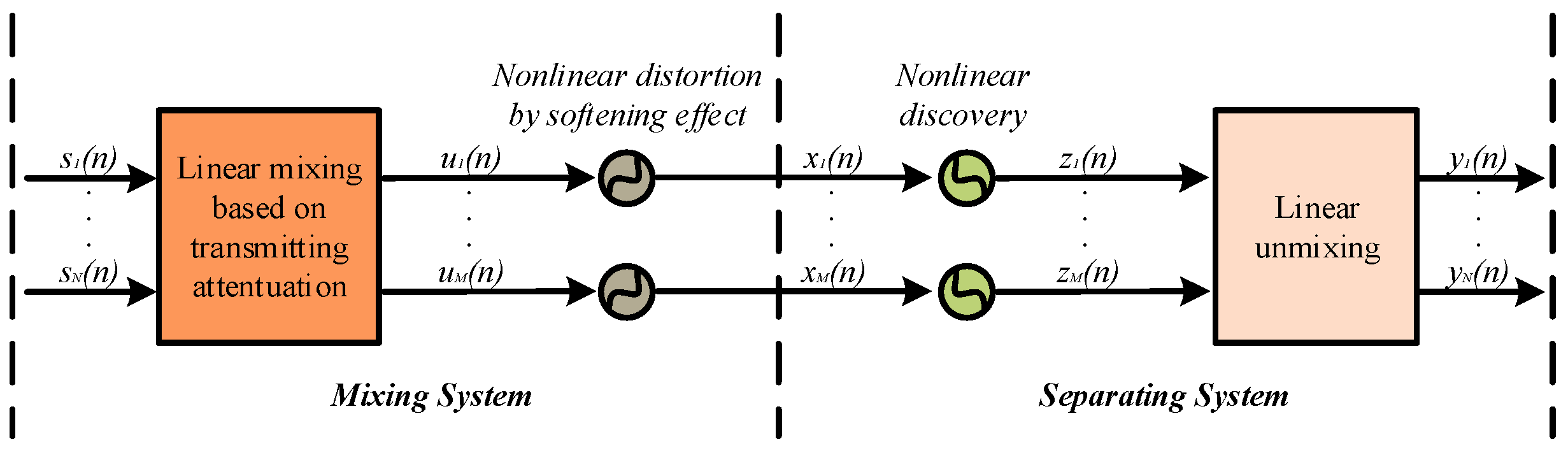
2.1. Nonlinear Underwater Acoustic Channel Model

It has been proven in [30,63] that bubbles in water have a softening effect on sound pressure, and a model of varying sound pressure was derived. The same model is therefore used in this paper. To simplify the discussion, only one-dimensional space is considered. Usually, it is assumed that bubbles have the same radius and are uniformly distributed in seawater. The model of the nonlinear distortion caused by the softening effect is derived from the wave equation and Rayleigh–Plesset equation:

$$\frac{{\partial }^{2}p(x,t)}{\partial x^2}-\frac{1}{c_{0l}^2}\frac{{\partial }^{2}p(x,t)}{\partial t^2}=-{\rho }_{0l}{N}_g\frac{{\partial }^{2}v(x,t)}{\partial t^2}$$

(1)

$$\begin{array}{cc}\hfill & \frac{{\partial }^{2}v(x,t)}{\partial t^2}+\delta {\omega }_{0g}\frac{\partial v(x,t)}{\partial t}+{\omega }_{0g}^{2}v(x,t)+\eta p(x,t)\hfill \\ \hfill & =av{(x,t)}^2+b\left(2v(x,t)\frac{{\partial }^{2}v(x,t)}{\partial t^2}+{\left(\frac{\partial v(x,t)}{\partial t}\right)}^2\right)\hfill \end{array}$$

(2)

In the equations above, $p(x,t)$ is the sound pressure, which varies with the coordinates and time, similar to the volume variation of bubbles $v(x,t)=V(x,t)-v_{0g}$, with the present volume $V(x,t)$ and the initial one $v_{0g}$, $v_{0g}=4\pi R_{0g}^3/3$, with the initial radius $R_{0g}$ of bubbles. $c_{0l}$ and ${\rho }_{0l}$ are, respectively, the sound speed in sea water and the density of the medium. $N_g$ is the number of bubbles per unit volume. $\delta$ denotes the viscous damping coefficient in sea water and ${\omega }_{0g}$ represents the resonance angular frequency of bubbles. $a=({\gamma }_g+1){\omega }_{0g}^2/\left(2v_{0g}\right)$, $b=1/\left(6v_{0g}\right)$ and $\eta =4\pi R_{0g}/{\rho }_{0l}$ are nonlinear coefficients defined to be convenient, in which ${\gamma }_g$ is the specific heat ratio. Using i and j as space and time indices, the first-order and second-order partial derivatives relative to time and coordinates can be converted into a discrete format and expressed as

$$\frac{{\partial }^2{p}_i}{\partial x^2}=\frac{p_{i+1}-2p_i+p_{i-1}}{h^2}$$

(3)

in which $p_i$ represents $p(x=i,t)$. Similarly, $p_j$ represents $p(x,t=j)$ and the in time domain

$$\begin{array}{cc}\hfill \frac{{\partial }^2{p}_j}{\partial t^2}& =\frac{p_{j+1}-2p_j+p_{j-1}}{{\tau }^2}\hfill \\ \hfill \frac{{\partial }^2{v}_j}{\partial t^2}& =\frac{v_{j+1}-2v_j+v_{j-1}}{{\tau }^2}\hfill \\ \hfill \frac{\partial p_j}{\partial t}& =\frac{p_j-p_{j-1}}{\tau }\hfill \\ \hfill \frac{\partial v_j}{\partial t}& =\frac{v_j-v_{j-1}}{\tau }\hfill \end{array}$$

(4)

in which h and $\tau$ are the space and time interval, respectively.

Finally, sound pressure in any coordinates and at any time can be derived as

$$\begin{array}{cc}\hfill p_{i,j+1}=& \left[{\tau }^2{p}_{i+1,j}+{\tau }^2{p}_{i-1,j}+2\left(\frac{h^2}{c_{0l}^2}-{\tau }^2\right)p_{i,j}-\frac{h^2}{c_{0l}^2}{p}_{i,j-1}\right.\hfill \\ \hfill & \left.-2{\rho }_{0l}{N}_g{h}^2{v}_{i,j}+{\rho }_{0l}{N}_g{h}^2{v}_{i,j-1}+{\rho }_{0l}{N}_g{h}^2{v}_{i,j+1}\right]/(h^2/c_{0l}^2)\hfill \end{array}$$

(5)

where the volume of bubbles at the same point is

$$\begin{array}{cc}\hfill v_{i,j+1}=& \left[(1-\delta {\omega }_{0g}\tau -b{v}_{i,j-1})v_{i,j-1}+\eta {\tau }^2{p}_{i,j}+(-a{\tau }^2+3b)v_{i,j}^2\right.\hfill \\ \hfill & \left.+(-2+\delta {\omega }_{0g}\tau +{\omega }_{0g}^2{\tau }^2)v_{i,j}\right]/(2b{v}_{i,j}-1)\hfill \end{array}$$

(6)

2.2. Nonlinear Mixing Model in BSS

In the BSS problem, the generic and instantaneous nonlinear mixing model can be defined as

$$X=\phi \left(S\right)$$

(7)

where $X={[x_1\left(n\right)x_2\left(n\right)\dots x_M\left(n\right)]}^T$ and $S={[s_1\left(n\right)s_2\left(n\right)\dots s_N\left(n\right)]}^T$ are M mixtures and N sources. $\phi (.)$ is a generic nonlinear mixing function. The purpose of nonlinear BSS is to find a nonlinear unmixing function $\psi (.)={\phi }^{-1}(.)$, which is the inverse of the mixing function, to recover the sources as precisely as possible by applying $Y=\psi \left(X\right)$.

Many types of nonlinear mixing models are used in BSS, such as the linear quadratic, bi-linear and post-nonlinear (PNL) models [64,65]. The PNL model is utilized in this paper and its structure is shown in Figure 1. In the mixing system, the sources are multiplied by an M-by-N mixing matrix to be linearly mixed based on transmitting attenuation before undergoing nonlinear distortion by softening effect. In the separating part, the observed signals are first nonlinearly recovered, which is the inverse of nonlinear distortion, and then linearly unmixed by an N-by-M matrix.

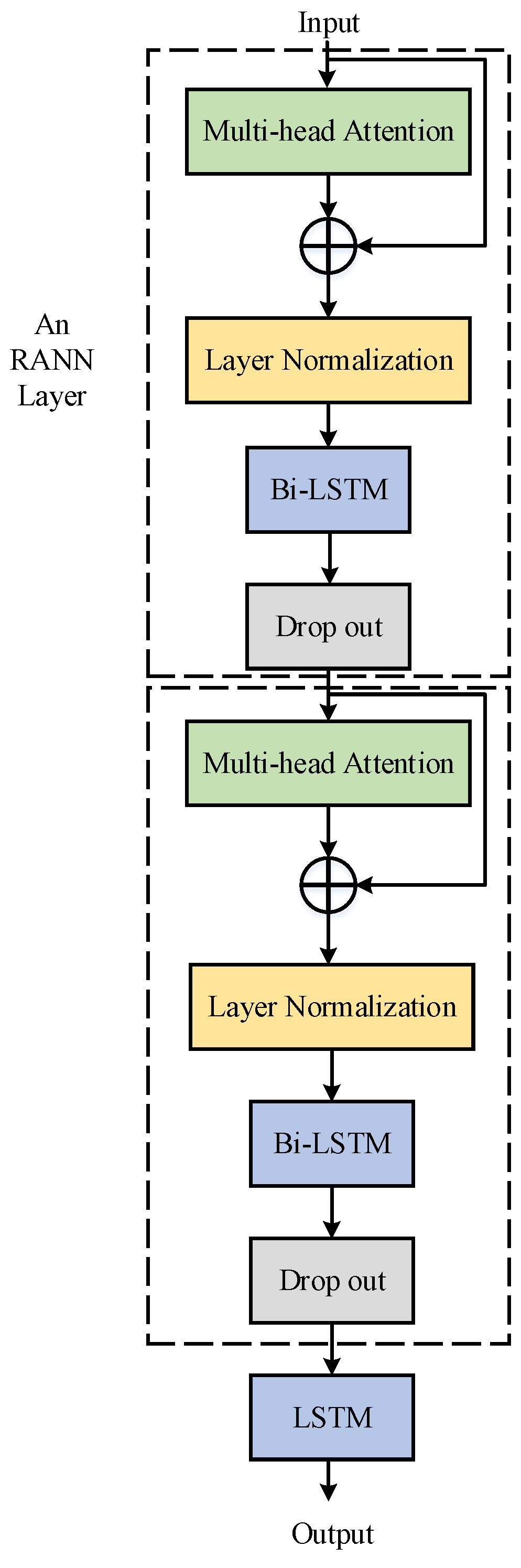
2.3. Recurrent Attention Neural Networks

Due to the advantages of RNNs in capturing local information and the Transformer’s excellent performance in acquiring global dependencies, a recurrent attention neural network (RANN) is designed in this paper, which is first utilized in nonlinear BSS. To achieve the recovery and separation of ship-radiated noise, the design of the network structure is as shown in Figure 2 and introduced as follows.

The multi-head attention mechanism shows the best performance in processing one-dimensional temporal signals and it has been applied in many fields. A multi-head attention layer is first used to process the input signals, which is followed by a residual connection and layer normalization. However, the attention mechanism performs weakly in acquiring the local information. Bi-LSTM has been proven to have excellent performance in nonlinear BSS [42] and it is successful in extracting the local information but weak in acquiring global information; thus, it could work well to complement the attention mechanism. As a result, a Bi-LSTM layer is then utilized in the network, which is followed by a drop-out layer to avoid overfitting. Then, the layer of the RANN is completed.

The recurrent attention process is repeated once to improve the performance, as it will be worse without the repetition. However, more repetitions are not necessary because this may heavily increase the number of parameters used but only slightly improve the performance, with more details shown in Section 4. An LSTM layer is finally used to obtain the separated results.

The whole procedure of signal processing is described as follows. The mixture signal is denoted as $X\in R^{M\times L}$, where M is the number of mixtures and L is the length of the signal in the time domain. Then, X is segmented into parts with length $Ns$ and, for convenience in training, the size of batch $bs$ is set. Thus, X is converted to $D\in R^{bn\times bs\times M\times Ns}$ with a permutation operation and $bn$ is the number of batches. The total $bn$ batches are divided into training, validation and testing sets in a proportion of 7:1:2 and used as inputs of the network for various purposes. In the simulation below, L is set to 500 and $Ns$ is set to 40 to simplify the calculation. There are 1000 samples of mixture data used in total and they are divided into various datasets with the proportion of 7:1:2.

Take the training progress as an example. The training batch $D_1\in R^{bs\times M\times Ns}$ is extended to h channels as features, $D_2\in R^{bs\times h\times Ns}$, before the attention mechanism, where h is the number of hidden elements in the attention and RNN layers. The shape of the feature tensors will not change until the LSTM layer, whose output is $D_n\in R^{bs\times N\times Ns}$, and N is the number of expected separated signals. Lastly, the outputs of the network are concatenated and recovered to $Y\in R^{N\times L}$. The progress is similar in the validation and testing stages.

3. Simulation Configuration

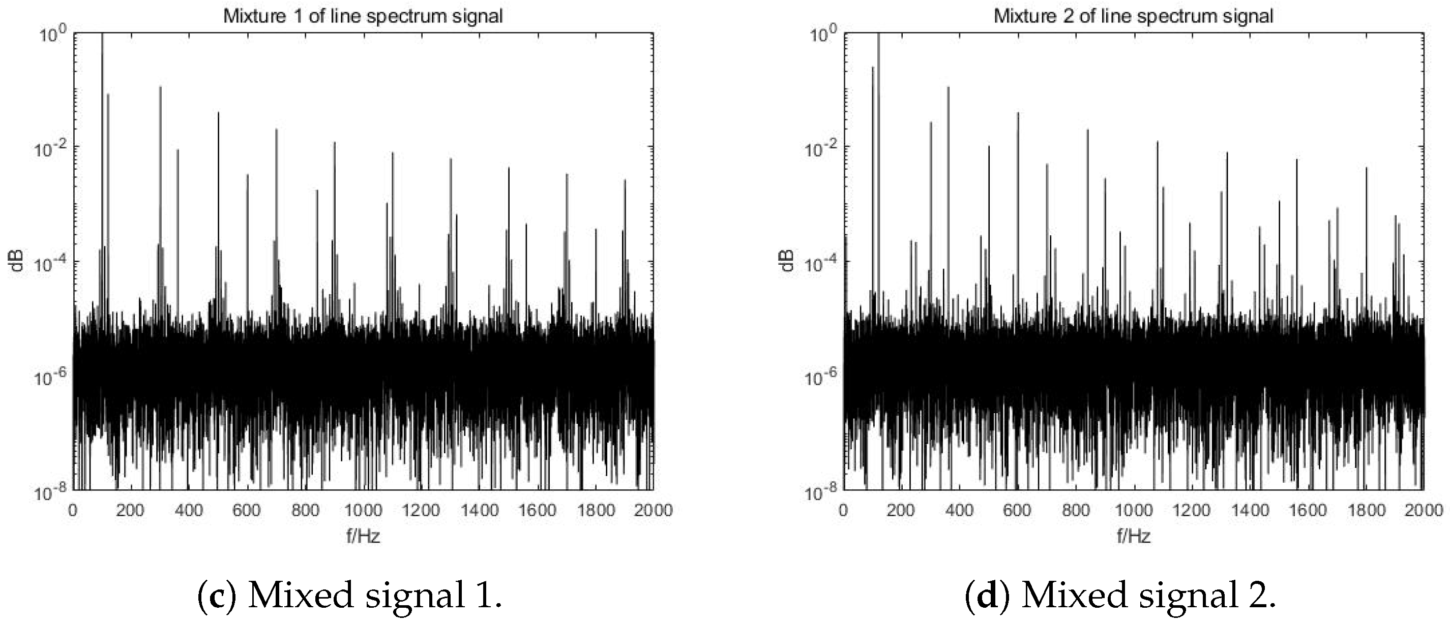
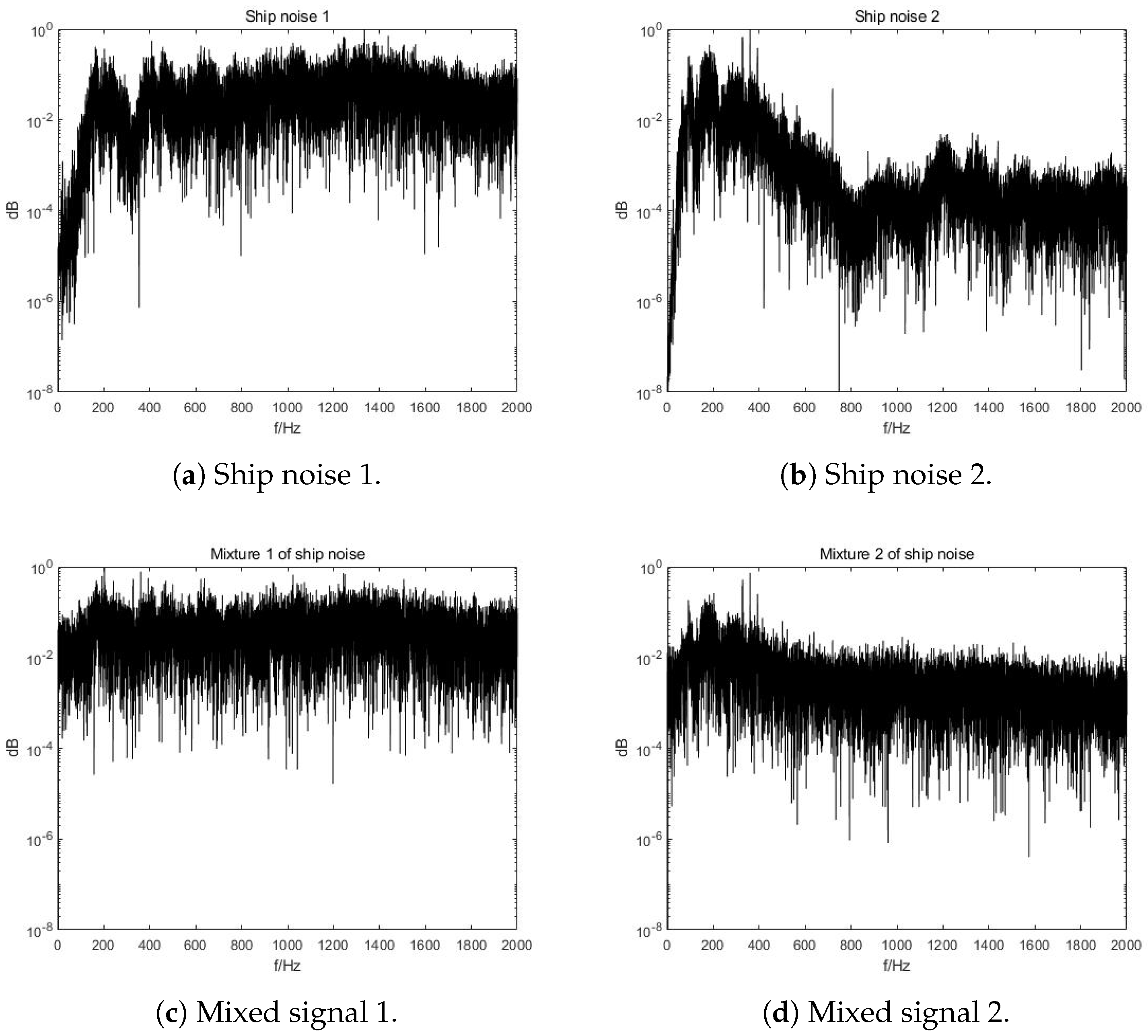
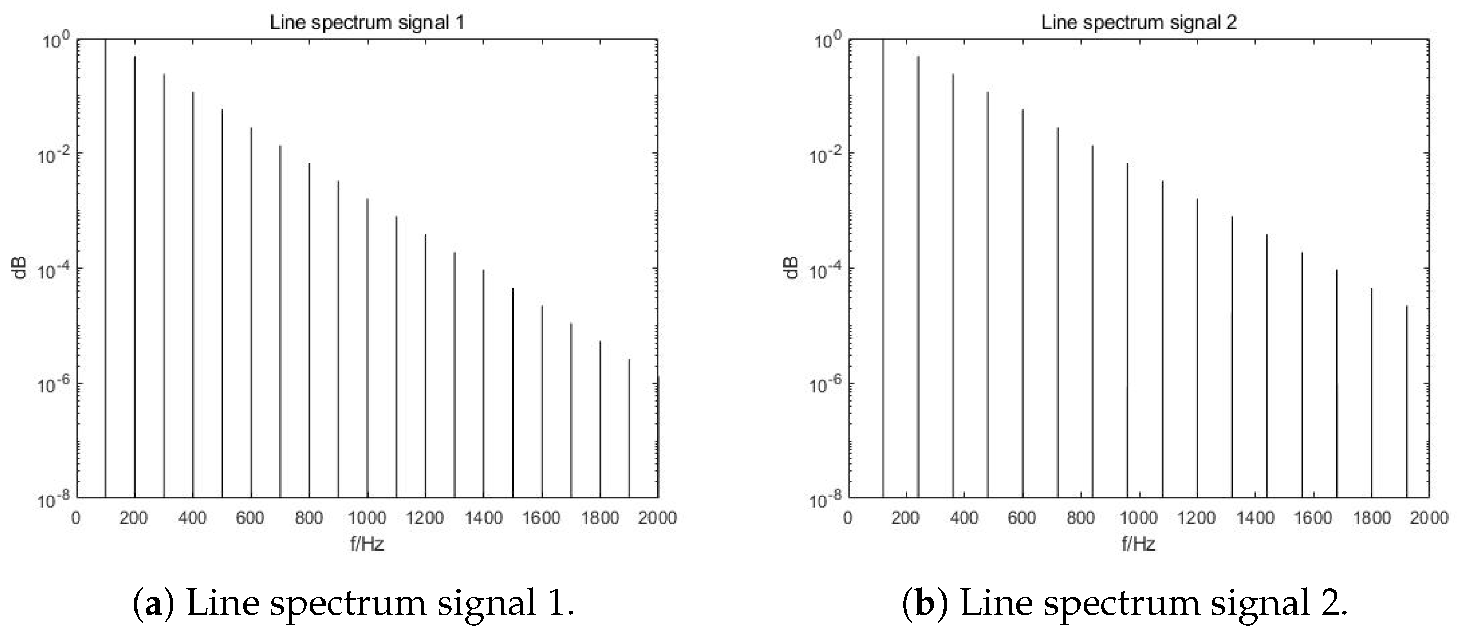
3.1. Original Signals, Distortion and Mixtures

To simplify the discussion, the smallest number of signals is selected, i.e., $m=n=2$ in Figure 1. To better validate the separation accuracy of the proposed network, the real recorded ship-radiated noise from the database ShipsEar [62] is used. Entries with index 6 and 22 are used as original signals, where the types of ships are passengers and ocean liners, respectively.

In order to maintain generality, various propagation distances are applied to the original signals, with 10 km for source $s1$ and 12 km for $s2$. Due to the fact that the propagation distance will influence the nonlinear distortion, as shown in Equations (5) and (6), nonlinear distorting functions will be different for various linear mixing signals $u\left(n\right)$ in Figure 1. For linear mixing matrix A, the coefficients are randomly selected and A must be fully ranked. When A equals $[0.45,0.13;0.21,0.43]$ and white Gaussian noise with 15 dB is added, the spectra of the original and mixed ship noise signals are as shown in Figure 3. It can be concluded from Figure 3 that the characteristics of the original ship noise are severely hidden in the mixture spectra. Only frequencies below 2 kHz are displayed as the ship-radiated noise is mainly distributed in this low-frequency region. This is used as the first dataset.

Due to the fact that ship-radiated noise consists of strong line spectra and weak continuous ones, and the former is the main basis of ship recognition [66,67], signals with line spectra are also generated as originals of the second dataset. Usually, a line spectrum consists of a fundamental frequency and resonance frequencies, with a strong relationship with the propeller shaft frequency and blade frequency. In this set of data, the fundamental frequencies are selected as 100 Hz and 120 Hz for both sources, and the amplitude attenuates as the frequency increases. Parameters used for the environment are the same as in the set of real ship noise discussed above. The spectra of the original and mixed signals are shown in Figure 4. A similar conclusion is obtained that the line spectra characteristics are heavily distorted in the mixtures.

3.2. Configuration and Referred Networks

In the proposed network, the output size of each recurrent unit is 256, as well as the number of hidden elements in the attention mechanism. The number of heads in attention is 8 and a $50\%$ dropping rate is used in each drop-out layer. The learning rate is set as ${10}^{-4}$ at the beginning and multiplies by $0.8$ after every 10 epochs, with a total of 100 epochs used in the training process. The Adam optimizer is also used to reduce the impact of the learning rate [68]. The mean square error (MSE) is used as the loss function and is displayed in Equation (8). The simulations are conducted on a Windows deep-learning server with 2 Intel(R) E5−2603 1.7 GHz CPUs (Santa Clara, CA, USA), 8 Samsung DDR4 16 GB RAM (Suwon, Republic of Korea) and 4 Nvidia GTX 1080Ti GPUs (Santa Clara, CA, USA).

The referred networks should be representative of different types. The candidate in [42], combining Bi-LSTM, LSTM and a drop-out layer, shows good performance in end-to-end nonlinear blind source separation, denoted as RNN in the description hereafter. The classical Transformer network [43] is another good candidate to test the performance and is denoted as Transformer. A recently published end-to-end U-net combining a CNN and multi-head attention, but used in linear BSS for music separation, is also selected as a referred network [47] and denoted as U-net. The total numbers of parameters used in the different networks are calculated by the Python package fvcore and shown in

Table 1. Number of parameters used in different networks.

Network	Parameters
RNN	0.3 M
Transformer	24 K
U-net	3.4 M
RANN (1 layer)	1.1 M
Proposed RANN (2 layers)	2.1 M
RANN (3 layers)	3.2 M
RANN (4 layers)	4.2 M

.

The metrics of the separation accuracy consist of the MSE, the correlation coefficient $\rho$ used in [69] and the signal-to-distortion ratio (SDR). The lower the MSE or the greater the $\rho$ and SDR, the better the performance. The metrics are calculated as follows and s and y represent the original signals and separated ones with length L:

$$MSE=\frac{1}{L}\sum _{i=1}^L{(s_i-y_i)}^2$$

(8)

$$\rho =\frac{{\sum }_{i=1}^L(s_i·y_i)}{{\sum }_{i=1}^L\left(\right|s_i|·|y_i\left|\right)}$$

(9)

$$SDR=10{log}_{10}\frac{{\sum }_{i=1}^L{(s_i-y_i)}^2}{{\sum }_{i=1}^L{s}_i^2}$$

(10)

4. Results and Discussion

4.1. Metrics of Results

The metrics of the separation results are shown in

Table 2. Separation results of different networks for ship-radiated noise.

Network	MSE	$\mathit{\rho }$	SDR (dB)
RNN	0.007	0.817	4.495
Transformer	0.037	0.001	−2.947
U-net	0.053	0.006	−4.453
RANN (1 layer)	0.007	0.830	4.492
Proposed RANN (2 layers)	0.006	0.840	4.651
RANN (3 layers)	0.006	0.842	4.674
RANN (4 layers)	0.006	0.843	4.684

and

Table 3. Separation results of different networks for line spectrum signals.

Network	MSE	$\mathit{\rho }$	SDR (dB)
RNN	0.035	0.929	8.621
Transformer	0.311	0.015	−0.842
U-net	0.504	−0.002	−2.939
RANN (1 layer)	0.020	0.967	11.003
Proposed RANN (2 layers)	0.014	0.981	12.699
RANN (3 layers)	0.013	0.987	12.850
RANN (4 layers)	0.012	0.992	12.922

. U-net performs the worst because it is designed for linear BSS and the nonlinear channel is not taken into account. The proposed network performs better than the RNN and Transformer because the RNN is successful in capturing local dependencies and the Transformer performs well in acquiring global ones. The RNN performs much better than the Transformer and slightly worse than the proposed network because the local dependencies are much stronger than the global relation in the considered underwater acoustic channels, as expressed in Equations (5) and (6). For the RANN with different layers of recurrent attention, the network with two layers is the best candidate because it performs much better than those with one layer, especially in line spectrum signal separation, and fewer parameters are used than in those with more layers.

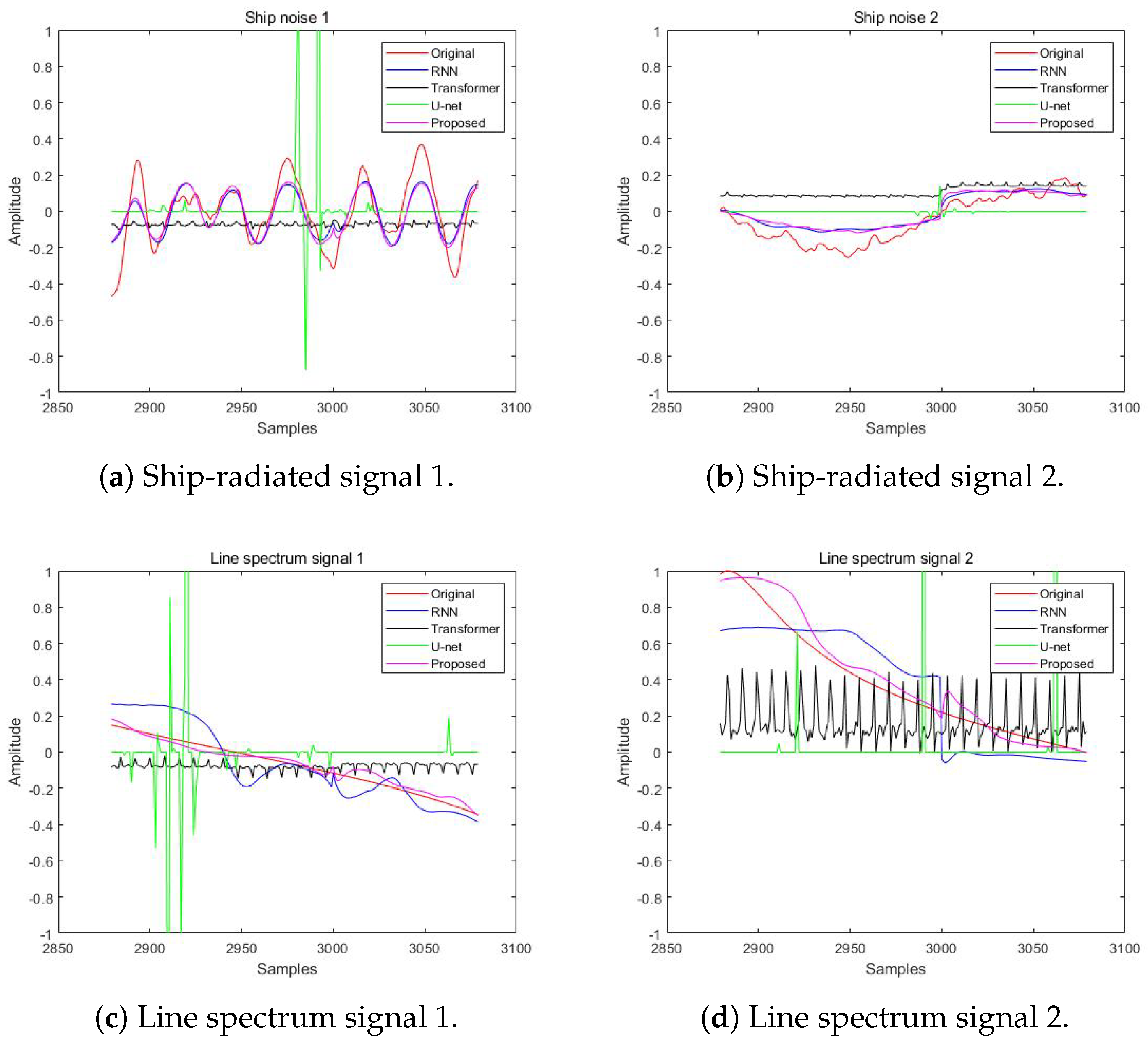
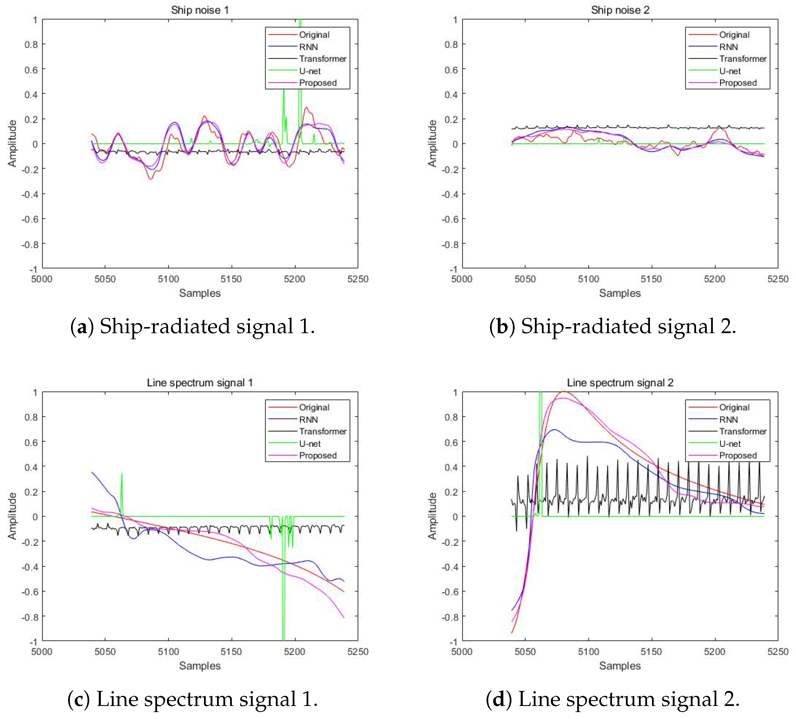
4.2. Separated Waveforms

The waveforms of the signals separated by different networks are displayed. By randomly selecting time segments, the original and separated ship-radiated noise from various networks is as shown in Figure 5 and Figure 6. In Figure 5, it can be seen that the waveform separated by the proposed network (in pink line) is slightly nearer the original waveform (in red line) than in those by the RNN (in blue line) and it performs much better than any other candidates. Conclusions can be made that, for ship noise, the proposed network separates them in with slightly higher accuracy than the RNN and is better than all others. For the line spectrum signals in Figure 6, the waveform separated by the proposed network (in pink line) shows the best performance with the least distortion from the original waveform (in red line) and it performs much better than any other method, including the RNN. In conclusion, the proposed network apparently works better than other candidates.

5. Conclusions

In this paper, the softening effect of bubbles in water is considered in underwater nonlinear blind ship-radiated noise separation, and an end-to-end recurrent attention neural network is proposed combining the advantages of the RNN and Transformer. According to the simulation results, high accuracy of separation is obtained by the proposal in terms of the MSE, correlation coefficient and SDR, compared with other networks including the RNN, Transformer and U-net, which are effective in other BSS scenes. It is found that the proposed scheme performs better than other candidates obviously in line spectrum signal separation and has a slight advantage over the RNN in separating the real ship noise. In the future, networks with greater compatibility with the underwater acoustic channel can be explored to obtain higher separation accuracy.

References

1. Yin, F.; Li, C.; Wang, H.; Nie, L.; Zhang, Y.; Liu, C.; Yang, F. Weak Underwater Acoustic Target Detection and Enhancement with BM-SEED Algorithm. J. Mar. Sci. Eng. 2023, 11, 357. [Google Scholar] [CrossRef]
2. Yin, F.; Li, C.; Wang, H.; Zhou, S.; Nie, L.; Zhang, Y.; Yin, H. A Robust Denoised Algorithm Based on Hessian-Sparse Deconvolution for Passive Underwater Acoustic Detection. J. Mar. Sci. Eng. 2023, 11, 2028. [Google Scholar] [CrossRef]
3. Chu, H.; Li, C.; Wang, H.; Wang, J.; Tai, Y.; Zhang, Y.; Yang, F.; Benezeth, Y. A deep-learning based high-gain method for underwater acoustic signal detection in intensity fluctuation environments. Appl. Acoust. 2023, 211, 109513. [Google Scholar] [CrossRef]
4. Zhou, M.; Wang, J.; Feng, X.; Sun, H.; Qi, J.; Lin, R. Neural-Network-Based Equalization and Detection for Underwater Acoustic Orthogonal Frequency Division Multiplexing Communications: A Low-Complexity Approach. Remote Sens. 2023, 15, 3796. [Google Scholar] [CrossRef]
5. Yonglin, Z.; Chao, L.; Haibin, W.; Jun, W.; Fan, Y.; Fabrice, M. Deep learning aided OFDM receiver for underwater acoustic communications. Appl. Acoust. 2022, 187, 108515. [Google Scholar] [CrossRef]
6. Wang, Z.; Li, Y.; Wang, C.; Ouyang, D.; Huang, Y. A-OMP: An Adaptive OMP Algorithm for Underwater Acoustic OFDM Channel Estimation. IEEE Wirel. Commun. Lett. 2021, 10, 1761–1765. [Google Scholar] [CrossRef]
7. Atanackovic, L.; Lampe, L.; Diamant, R. Deep-Learning Based Ship-Radiated Noise Suppression for Underwater Acoustic OFDM Systems. In Proceedings of the Global Oceans 2020: Singapore—U.S. Gulf Coast, Biloxi, MS, USA, 5–30 October 2020; pp. 1–8. [Google Scholar] [CrossRef]
8. Li, P.; Zhang, X.G.; Zhang, X.Y.; Liu, Y. Vertical array signal recovery method based on normalized virtual time reversal mirror. J. Phys. Conf. Ser. 2023, 2486, 012070. [Google Scholar] [CrossRef]
9. Yuqing, Y.; Peng, X.; Nikos, D. Underwater localization with binary measurements: From compressed sensing to deep unfolding. Digit. Signal Process. 2023, 133, 103867. [Google Scholar] [CrossRef]
10. Zonglong, B. Sparse Bayesian learning for sparse signal recovery using l1/2-norm. Appl. Acoust. 2023, 207, 109340. [Google Scholar] [CrossRef]
11. Zhu, J.H.; Fan, C.Y.; Song, Y.P.; Huang, X.T.; Zhang, B.B.; Ma, Y.X. Coordination of Complementary Sets for Low Doppler-Induced Sidelobes. Remote Sens. 2022, 14, 1549. [Google Scholar] [CrossRef]
12. Zhu, J.H.; Song, Y.P.; Jiang, N.; Xie, Z.; Fan, C.Y.; Huang, X.T. Enhanced Doppler Resolution and Sidelobe Suppression Performance for Golay Complementary Waveforms. Remote Sens. 2023, 15, 2452. [Google Scholar] [CrossRef]
13. Xie, Z.; Xu, Z.; Han, S.; Zhu, J.; Huang, X. Modulus Constrained Minimax Radar Code Design Against Target Interpulse Fluctuation. IEEE Trans. Veh. Technol. 2023, 72, 13671–13676. [Google Scholar] [CrossRef]
14. Zhang, X.B.; Wu, H.R.; Sun, H.X.; Ying, W.W. Multireceiver SAS Imagery Based on Monostatic Conversion. IEEE J. Sel. Top. Appl. Earth Obs. Remote Sens. 2021, 14, 10835–10853. [Google Scholar] [CrossRef]
15. Zhang, X.B.; Yang, P.X.; Zhou, M.Z. Multireceiver SAS Imagery With Generalized PCA. IEEE Geosci. Remote Sens. Lett. 2023, 20, 1502205. [Google Scholar] [CrossRef]
16. Cherry, E.C. Some experiments on the recognition of speech, with one and with two ears. J. Acoust. Soc. Am. 1953, 25, 975–979. [Google Scholar] [CrossRef]
17. Zhang, W.; Tait, A.; Huang, C.; Ferreira de Lima, T.; Bilodeau, S.; Blow, E.C.; Jha, A.; Shastri, B.J.; Prucnal, P. Broadband physical layer cognitive radio with an integrated photonic processor for blind source separation. Nat. Commun. 2023, 14, 1107. [Google Scholar] [CrossRef] [PubMed]
18. Kumari, R.; Mustafi, A. The spatial frequency domain designated watermarking framework uses linear blind source separation for intelligent visual signal processing. Front. Neurorobot. 2022, 16, 1054481. [Google Scholar] [CrossRef] [PubMed]
19. Erdogan, A.T. An Information Maximization Based Blind Source Separation Approach for Dependent and Independent Sources. In Proceedings of the ICASSP 2022—2022 IEEE International Conference on Acoustics, Speech and Signal Processing (ICASSP), Singapore, 23–27 May 2022; pp. 4378–4382. [Google Scholar] [CrossRef]
20. Boccuto, A.; Gerace, I.; Giorgetti, V.; Valenti, G. A Blind Source Separation Technique for Document Restoration Based on Image Discrete Derivative. In International Conference on Computational Science and Its Applications; Springer: Berlin/Heidelberg, Germany, 2022; pp. 445–461. [Google Scholar]
21. Martin, G.; Hooper, A.; Wright, T.J.; Selvakumaran, S. Blind Source Separation for MT-InSAR Analysis with Structural Health Monitoring Applications. IEEE J. Sel. Top. Appl. Earth Obs. Remote Sens. 2022, 15, 7605–7618. [Google Scholar] [CrossRef]
22. Yao, H.; Wang, H.; Zhang, Z.; Xu, Y.; Juergen, K. A stochastic nonlinear differential propagation model for underwater acoustic propagation: Theory and solution. Chaos Solitons Fractals 2021, 150, 111105. [Google Scholar]
23. Naman, H.A.; Abdelkareem, A.E. Variable direction-based self-interference full-duplex channel model for underwater acoustic communication systems. Int. J. Commun. Syst. 2022, 35, e5096. [Google Scholar] [CrossRef]
24. Shen, L.; Henson, B.; Zakharov, Y.; Mitchell, P. Digital Self-Interference Cancellation for Full-Duplex Underwater Acoustic Systems. IEEE Trans. Circuits Syst. II Express Briefs 2020, 67, 192–196. [Google Scholar] [CrossRef]
25. Yang, S.; Deane, G.B.; Preisig, J.C.; Sevüktekin, N.C.; Choi, J.W.; Singer, A.C. On the Reusability of Postexperimental Field Data for Underwater Acoustic Communications R&D. IEEE J. Ocean. Eng. 2019, 44, 912–931. [Google Scholar] [CrossRef]
26. Ma, X.; Raza, W.; Wu, Z.; Bilal, M.; Zhou, Z.; Ali, A. A Nonlinear Distortion Removal Based on Deep Neural Network for Underwater Acoustic OFDM Communication with the Mitigation of Peak to Average Power Ratio. Appl. Sci. 2020, 10, 4986. [Google Scholar] [CrossRef]
27. Campo-Valera, M.; Rodríguez-Rodríguez, I.; Rodríguez, J.V.; Herrera-Fernández, L.J. Proof of Concept of the Use of the Parametric Effect in Two Media with Application to Underwater Acoustic Communications. Electronics 2023, 12, 3459. [Google Scholar] [CrossRef]
28. Yao, H.; Wang, H.; Xu, Y.; Juergen, K. A recurrent plot based stochastic nonlinear ray propagation model for underwater signal propagation. New J. Phys. 2020, 22, 063025. [Google Scholar]
29. Cheng, Y.; Shi, J.; Deng, A. Effective Nonlinearity Parameter and Acoustic Propagation Oscillation Behavior in Medium of Water Containing Distributed Bubbles. In Proceedings of the 2021 OES China Ocean Acoustics (COA), Harbin, China, 14–17 July 2021; IEEE: Piscataway, NJ, USA, 2021; pp. 345–350. [Google Scholar]
30. Yu, J.; Yang, D.; Shi, J. Influence of softening effect of bubble water on cavity resonance. In Proceedings of the 2021 OES China Ocean Acoustics (COA), Harbin, China, 14–17 July 2021; IEEE: Piscataway, NJ, USA, 2021; pp. 351–355. [Google Scholar]
31. Li, J.; Yang, D.; Chen, G. Study on the acoustic scattering characteristics of the parametric array in the wake field of underwater cylindrical structures. In Proceedings of the 2021 OES China Ocean Acoustics (COA), Harbin, China, 14–17 July 2021; IEEE: Piscataway, NJ, USA, 2021; pp. 340–344. [Google Scholar]
32. Li, D.; Wu, M.; Yu, L.; Han, J.; Zhang, H. Single-channel blind source separation of underwater acoustic signals using improved NMF and FastICA. Front. Mar. Sci. 2023, 9, 1097003. [Google Scholar] [CrossRef]
33. Khosravy, M.; Gupta, N.; Dey, N.; Crespo, R.G. Underwater IoT network by blind MIMO OFDM transceiver based on probabilistic Stone’s blind source separation. ACM Trans. Sens. Netw. (TOSN) 2022, 18, 1–27. [Google Scholar] [CrossRef]
34. Zhang, W.; Li, X.; Zhou, A.; Ren, K.; Song, J. Underwater acoustic source separation with deep Bi-LSTM networks. In Proceedings of the 2021 4th International Conference on Information Communication and Signal Processing (ICICSP), Shanghai, China, 24–26 September 2021; pp. 254–258. [Google Scholar] [CrossRef]
35. Chen, J.; Liu, C.; Xie, J.; An, J.; Huang, N. Time–Frequency Mask-Aware Bidirectional LSTM: A Deep Learning Approach for Underwater Acoustic Signal Separation. Sensors 2022, 22, 5598. [Google Scholar] [CrossRef]
36. Hadi, F.I.M.A.; Ramli, D.A.; Azhar, A.S. Passive Acoustic Monitoring (PAM) of Snapping Shrimp Sound Based on Blind Source Separation (BSS) Technique. In Proceedings of the 11th International Conference on Robotics, Vision, Signal Processing and Power Applications: Enhancing Research and Innovation through the Fourth Industrial Revolution; Springer: Berlin/Heidelberg, Germany, 2022; pp. 605–611. [Google Scholar]
37. Hadi, F.I.M.; Ramli, D.A.; Hassan, N. Spiny Lobster Sound Identification Based on Blind Source Separation (BSS) for Passive Acoustic Monitoring (PAM). Procedia Comput. Sci. 2021, 192, 4493–4502. [Google Scholar] [CrossRef]
38. Deville, Y.; Faury, G.; Achard, V.; Briottet, X. An NMF-based method for jointly handling mixture nonlinearity and intraclass variability in hyperspectral blind source separation. Digit. Signal Process. 2023, 133, 103838. [Google Scholar] [CrossRef]
39. Isomura, T.; Toyoizumi, T. On the achievability of blind source separation for high-dimensional nonlinear source mixtures. Neural Comput. 2021, 33, 1433–1468. [Google Scholar] [CrossRef]
40. Moraes, C.P.; Fantinato, D.G.; Neves, A. Epanechnikov kernel for PDF estimation applied to equalization and blind source separation. Signal Process. 2021, 189, 108251. [Google Scholar] [CrossRef]
41. He, J.; Chen, W.; Song, Y. Single channel blind source separation under deep recurrent neural network. Wirel. Pers. Commun. 2020, 115, 1277–1289. [Google Scholar] [CrossRef]
42. Zamani, H.; Razavikia, S.; Otroshi-Shahreza, H.; Amini, A. Separation of Nonlinearly Mixed Sources Using End-to-End Deep Neural Networks. IEEE Signal Process. Lett. 2020, 27, 101–105. [Google Scholar] [CrossRef]
43. Vaswani, A.; Shazeer, N.; Parmar, N.; Uszkoreit, J.; Jones, L.; Gomez, A.N.; Kaiser, L.u.; Polosukhin, I. Attention is All you Need. In Advances in Neural Information Processing Systems; Guyon, I., Luxburg, U.V., Bengio, S., Wallach, H., Fergus, R., Vishwanathan, S., Garnett, R., Eds.; Curran Associates, Inc.: Red Hook, NY, USA, 2017; Volume 30, pp. 1–11. [Google Scholar]
44. Ansari, S.; Alnajjar, K.A.; Khater, T.; Mahmoud, S.; Hussain, A. A Robust Hybrid Neural Network Architecture for Blind Source Separation of Speech Signals Exploiting Deep Learning. IEEE Access 2023, 11, 100414–100437. [Google Scholar] [CrossRef]
45. Herzog, A.; Chetupalli, S.R.; Habets, E.A.P. AmbiSep: Ambisonic-to-Ambisonic Reverberant Speech Separation Using Transformer Networks. In Proceedings of the 2022 International Workshop on Acoustic Signal Enhancement (IWAENC), Bamberg, Germany, 5–8 September 2022; pp. 1–5. [Google Scholar] [CrossRef]
46. Qian, J.; Liu, X.; Yu, Y.; Li, W. Stripe-Transformer: Deep stripe feature learning for music source separation. EURASIP J. Audio Speech Music. Process. 2023, 2023, 2. [Google Scholar] [CrossRef]
47. Wang, J.; Liu, H.; Ying, H.; Qiu, C.; Li, J.; Anwar, M.S. Attention-based neural network for end-to-end music separation. CAAI Trans. Intell. Technol. 2023, 8, 355–363. [Google Scholar] [CrossRef]
48. Reddy, P.; Wisdom, S.; Greff, K.; Hershey, J.R.; Kipf, T. AudioSlots: A slot-centric generative model for audio separation. arXiv 2023, arXiv:2305.05591. [Google Scholar]
49. Subakan, C.; Ravanelli, M.; Cornell, S.; Grondin, F.; Bronzi, M. Exploring Self-Attention Mechanisms for Speech Separation. IEEE/ACM Trans. Audio Speech Lang. Process. 2023, 31, 2169–2180. [Google Scholar] [CrossRef]
50. Melissaris, T.; Schenke, S.; Van Terwisga, T.J. Cavitation erosion risk assessment for a marine propeller behind a Ro–Ro container vessel. Phys. Fluids 2023, 35, 013342. [Google Scholar] [CrossRef]
51. Abbasia, A.A.; Viviania, M.; Bertetta, D.; Delucchia, M.; Ricottic, R.; Tania, G. Experimental Analysis of Cavitation Erosion on Blade Root of Controlable Pitch Propeller. In Proceedings of the 20th International Conference on Ship & Maritime Research, Genoa, La Spazia, Italy, 15–17 June 2022; pp. 254–262. [Google Scholar]
52. Wang, Y.; Zhang, H.; Huang, W. Fast ship radiated noise recognition using three-dimensional mel-spectrograms with an additive attention based transformer. Front. Mar. Sci. 2023, 1–15. [Google Scholar] [CrossRef]
53. Pu, X.; Yi, P.; Chen, K.; Ma, Z.; Zhao, D.; Ren, Y. EEGDnet: Fusing non-local and local self-similarity for EEG signal denoising with transformer. Comput. Biol. Med. 2022, 151, 106248:1–106248:9. [Google Scholar] [CrossRef] [PubMed]
54. Woo, B.J.; Kim, H.Y.; Kim, J.; Kim, N.S. Speech separation based on dptnet with sparse attention. In Proceedings of the 2021 7th IEEE International Conference on Network Intelligence and Digital Content (IC-NIDC), Beijing, China, 17–19 November 2021; IEEE: Piscataway, NJ, USA, 2021; pp. 339–343. [Google Scholar]
55. Liu, Y.; Xu, X.; Tu, W.; Yang, Y.; Xiao, L. Improving Acoustic Echo Cancellation by Mixing Speech Local and Global Features with Transformer. In Proceedings of the ICASSP 2023—2023 IEEE International Conference on Acoustics, Speech and Signal Processing (ICASSP), Rhodes Island, Greece, 4–10 June 2023; IEEE: Piscataway, NJ, USA, 2023; pp. 1–5. [Google Scholar]
56. Yin, J.; Liu, A.; Li, C.; Qian, R.; Chen, X. A GAN Guided Parallel CNN and Transformer Network for EEG Denoising. IEEE J. Biomed. Health Inform. 2023, 1–12, Early Access. [Google Scholar] [CrossRef] [PubMed]
57. Ji, W.; Yan, G.; Li, J.; Piao, Y.; Yao, S.; Zhang, M.; Cheng, L.; Lu, H. DMRA: Depth-induced multi-scale recurrent attention network for RGB-D saliency detection. IEEE Trans. Image Process. 2022, 31, 2321–2336. [Google Scholar] [CrossRef] [PubMed]
58. Reza, S.; Ferreira, M.C.; Machado, J.J.M.; Tavares, J.M.R. A multi-head attention-based transformer model for traffic flow forecasting with a comparative analysis to recurrent neural networks. Expert Syst. Appl. 2022, 202, 117275. [Google Scholar] [CrossRef]
59. Geng, X.; He, X.; Xu, L.; Yu, J. Graph correlated attention recurrent neural network for multivariate time series forecasting. Inf. Sci. 2022, 606, 126–142. [Google Scholar] [CrossRef]
60. De Maissin, A.; Vallée, R.; Flamant, M.; Fondain-Bossiere, M.; Le Berre, C.; Coutrot, A.; Normand, N.; Mouchère, H.; Coudol, S.; Trang, C.; et al. Multi-expert annotation of Crohn’s disease images of the small bowel for automatic detection using a convolutional recurrent attention neural network. Endosc. Int. Open 2021, 9, E1136–E1144. [Google Scholar] [CrossRef] [PubMed]
61. Zhang, X.; Gao, X.; Lu, W.; He, L.; Li, J. Beyond vision: A multimodal recurrent attention convolutional neural network for unified image aesthetic prediction tasks. IEEE Trans. Multimed. 2020, 23, 611–623. [Google Scholar] [CrossRef]
62. Santos-Domínguez, D.; Torres-Guijarro, S.; Cardenal-López, A.; Pena-Gimenez, A. ShipsEar: An underwater vessel noise database. Appl. Acoust. 2016, 113, 64–69. [Google Scholar] [CrossRef]
63. Yu, J.; Yang, D.; Shi, J.; Zhang, J.; Fu, X. Nonlinear sound field under bubble softening effect. J. Harbin Eng. Univ. 2023, 44, 1433–1444. [Google Scholar]
64. Deville, Y.; Duarte, L.T.; Hosseini, S. Nonlinear Blind Source Separation and Blind Mixture Identification: Methods for Bilinear, Linear-Quadratic and Polynomial Mixtures; Springer: Berlin/Heidelberg, Germany, 2021. [Google Scholar]
65. Moraes, C.P.; Saldanha, J.; Neves, A.; Fantinato, D.G.; Attux, R.; Duarte, L.T. An SOS-Based Algorithm for Source Separation in Nonlinear Mixtures. In Proceedings of the 2021 IEEE Statistical Signal Processing Workshop (SSP), Rio de Janeiro, Brazil, 11–14 July 2021; IEEE: Piscataway, NJ, USA, 2021; pp. 156–160. [Google Scholar]
66. Wang, H.; Guo, L. Research of Modulation Feature Extraction from Ship-Radiated Noise. Proc. J. Phys. Conf. Ser. 2020, 1631, 012130. [Google Scholar] [CrossRef]
67. Peng, C.; Yang, L.; Jiang, X.; Song, Y. Design of a ship radiated noise model and its application to feature extraction based on winger’s higher-order spectrum. In Proceedings of the 2019 IEEE 4th Advanced Information Technology, Electronic and Automation Control Conference (IAEAC), Chengdu, China, 20–22 December 2019; IEEE: Piscataway, NJ, USA, 2019; Volume 1, pp. 582–587. [Google Scholar] [CrossRef]
68. Kingma, D.P.; Ba, J. Adam: A method for stochastic optimization. arXiv 2014, arXiv:1412.6980. [Google Scholar]
69. Cao, Y.; Zhang, H.; Qin, Y.; Zhu, H.; Cao, J.; Ma, N. Joint Denoising Blind Source Separation Algorithmfor Anti-jamming. In Proceedings of the 2021 4th International Conference on Information Communication and Signal Processing (ICICSP), Shanghai, China, 24–26 September 2021; IEEE: Piscataway, NJ, USA, 2021; pp. 27–35. [Google Scholar] [CrossRef]
Figure 1. The sketch of the PNL model used in this paper.
Remotesensing 16 00653 g001
Figure 2. The model of the proposed recurrent attention neural network, containing two layers of recurrent attention neural network and an LSTM layer.
Remotesensing 16 00653 g002
Figure 3. Spectra of original and mixed ship noise, with characteristics severely hidden in the mixture spectra.
Remotesensing 16 00653 g003
Figure 4. Spectra of original and mixed line spectrum signals, with line spectra characteristics heavily distorted in mixtures.
Remotesensing 16 00653 g004aRemotesensing 16 00653 g004b
Figure 5. Fragment 1 of original and separated waveform, with the proposed network performing the best.
Remotesensing 16 00653 g005
Figure 6. Fragment 2 of original and separated waveform, with the proposed network performing the best.
Remotesensing 16 00653 g006