1. Introduction
Soil represents a complex mixture of organic and inorganic constituents with different physical and chemical properties, which vary significantly between locations and even within a single field [
1]. It is a key component of terrestrial ecosystems, as it facilitates the circulation of energy and materials between the atmosphere and the biosphere [
2].
Soil health can be defined as the ability of the soil to function effectively as a component in a thriving ecosystem [
3]. In order to ensure effective monitoring and enable adequate assessment of the condition of the soil, one needs to select appropriate indicators of its condition. The indicators should meet certain criteria: they should be accepted by experts as valid; their measurement should be carried out routinely and on a large scale; they need to be understood and accepted by the general population in order to achieve a global impact [
4].
Soil organic carbon (SOC) content is a widely accepted indicator of soil quality, as SOC plays a central role in various soil functions [
5]. SOC measurement is a common component of soil property analysis. Furthermore, carbon as an element is well known and recognized by the global population [
6]. All of this makes SOC a valuable indicator for assessing and monitoring changes in soil health.
The amount and quality of SOC are closely related to key soil functions, including nutrient mineralization, aggregate stability, air and water permeability, water retention, and flood control ability [
5]. These soil functions are, in turn, related to a wide range of ecosystem attributes. For example, high SOC levels in mineral soils tend to correlate with high plant productivity, which has a positive effect on wildlife habitat, distribution, and population size [
7]. Through the protection and increase of stored SOC, one can protect or increase soil fertility, reduce soil erosion, and reduce habitat conversions [
8].
In addition to its importance for the soil, SOC has the potential to help neutralize the negative effects of increasing concentrations of CO
2 in the atmosphere (which significantly contribute to global warming and climate change [
9]) and help ensure food security around the wold [
10].
While SOC plays a key role in mitigating climate change by acting as a carbon sink, the historical loss of carbon from this pool [
11] has been significant, and the potential for future accelerated loss under warming scenarios is a serious threat [
12,
13].
As a natural solution to fight climate change, strategies that involve conserving existing SOC stocks (avoidance of losses) and replenishing stocks in carbon-depleted soils [
14] can be used as a means of achieving the United Nations Sustainable Development Goals (UNSDG), the goals of the United Nations Framework Convention on Climate Change (UNFCCC), and the United Nations Convention on Combating Desertification (UNCCD) [
15].
Despite the scientific consensus about the potential and myriad benefits that can be brought about by the development and application of soil organic carbon storage and sequestration techniques, they remain limited in practice. A fundamental issue affecting the adoption of such methodologies is the lack of accurate and cost-effective ways of measuring SOC content in the top layer of the soil (as this is most affected by land use, agricultural practices, etc.).
When it comes to measuring global SOC stocks, many estimates have been published over the past decades, and most studies report a global SOC estimate of approximately 1500 Pg of carbon (Pg C), but there is considerable variation among estimates (ranging from 504 to 3000 Pg C) [
16].
The large variation in the estimates of global SOC stocks arises from differences in the sampling period, the intensity and spatial resolution of soil profile databases, as well as from differences in approaches to calculating the estimates themselves [
17]. The uneven distribution of georeferenced soil profiles around the world is another reason for such a large variation in the estimates [
18]. In addition, there is no consensus when it comes to including inorganic carbon, different levels of rock content [
19], and the effects of natural or anthropogenic phenomena (such as flooding, erosion, fire, soil fertilization, and plowing [
20]) in carbon stock assessments.
If we are to move forward in understanding and managing SOC for the benefit of humanity as a whole, effective and efficient methodologies for continuous monitoring of SOC on a global scale are needed.
Unfortunately, traditional methodologies employed in monitoring SOC tend to be labor-intensive, costly, and impractical [
21]. These procedures entail comprehensive soil sampling campaigns, subsequent laboratory testing, and extensive data processing [
22] to obtain what can truly be labeled as “ground truth” data.
In this study, we aimed to determine the soil organic content (SOC) of agricultural fields using Sentinel-2 satellite imagery, which provides spatially continuous and cost-effective data about the state of the Earth’s surface. To achieve this, we used machine learning techniques, which require a dataset of satellite images and corresponding SOC measurements collected through field sampling, on which to train and validate our models.
2. Background and Related Work
In recent years, remote sensing has emerged as a particularly effective method for tracking agricultural and environmental changes [
23,
24,
25,
26]. The technology relies on diverse sensors and platforms, such as satellite constellations and Unmanned Aerial Systems (UAS) to gather data, which are then typically processed using advanced algorithms, often in the realm of machine learning (ML) and deep learning (DL) [
27].
Deep learning represents a specialized subset of machine learning that excels at learning from large, unstructured datasets using complex, layered neural networks. While traditional ML algorithms work well with smaller, structured datasets and often require manual feature selection, DL algorithms automatically extract features and patterns, especially from data like images and speech. This makes deep learning more powerful for certain applications, but it requires more computational resources and is often less interpretable than conventional machine learning techniques.
The ongoing advancements in remote sensing represent a promising alternative to traditional SOC monitoring. Toth and Jóžków provide a fairly recent review of different remote sensing platforms and sensors available today [
28].
In the study presented here, the focus is on inferring SOC content from satellite data only. Most studies focused on determining SOC, however, rely on data (spectrograms) collected from hand-held sensors. While the accuracy achieved in this way is typically higher than using satellite imagery, such approaches can hardly be scaled to enable continuous monitoring of carbon stocks on a global level.
Gomez et al. [
29] presented an early, albeit limited study (based on just 146 soil samples), which compared the results that can be achieved applying ML methods to in-the-field Vis–NIR measurements vs. applying them to hyperspectral satellite imagery. The images were obtained from the Hyperion sensor on the EO-1 satellite, which is, unfortunately, no longer functional, and there is no longer an active hyperspectral satellite that captures images in the VNIR–SWIR region, making it hard to replicate their work. In addition to trying to model the whole dataset used in the study, the authors tried focusing on specific land cover classes (cropping soils, pasture soils) and opted for a partial least-squares regression as their SOC predictor. Gomez et al. observed that the SOC in their cropping soils ranged between 0.54% and 1% and was lower than in the pastures, where SOC was in the 1.08% to 5.1% range. They evaluated their methodology based on R
2 and the Root-Mean-Squared Error (RMSE). The models based on satellite imagery did not perform well for cropping soils (R
2 of 0.04 and RMSE of 0.11) and lagged significantly behind the hand-held-sensor-based models in terms of R
2 (R
2 of 0.16 and RMSE of 0.1). However, when evaluated on pastures and the whole dataset, the two approaches achieved comparable and much better performance. The approach based solely on satellite data at their native resolution achieved an R
2 of 0.51, but the RMSE was quite high (0.73% SOC). Thus, the study showed that land cover is very important, when it comes to modeling and estimating SOC remotely.
More recently, Wang et al. [
30] tried to use ML techniques to estimate SOC stock in the semi-arid rangelands of eastern Australia through the application of different machine learning techniques, with a focus on evaluating the impact of considering seasonal fractional cover on model performance. These features were used to extend other hand-crafted features derived from satellite imagery, as well as other remotely sensed climate features such as rainfall and temperature and data about lithology. They trained and evaluated their models using a limited amount of soil samples (705). They used random forests (RF) [
31], Boosted Regression Trees (BRT) [
32], and support vector machines (SVM) [
33] to model their data. The RF approach performed the best and achieved an R
2 of 0.47 on their dataset.
Several studies tried to evaluate the effectiveness of hyperspectral data obtained from airborne sensors and extended their findings to evaluate the expected performance of sensors expected to be deployed in the future [
34,
35]. While we focus on multispectral data in the study presented here, it is worth noting that, albeit relying on a very limited set of soil samples (81) obtained for a 7 km
2 area in Luxembourg, 40% of which were used as a test set, Steinberg et al. achieved a relatively high R
2 (0.74) and an RMSE of 0.22% for SOC using autoPSLR applied to hyperspectral data from an airborne sensor [
35]. Once sufficient hyperspectral data are available, the methodology we propose can easily be adapted to that domain, leading to even better performance.
Over the last decade, deep learning has revolutionized the area of machine learning and artificial intelligence and has become the dominant paradigm in the domain. The crucial advance over previously used methods is that the approach relies on end-to-end learning, which allows the ML models to learn the features on which to make their decisions and estimated directly from the raw input data, instead of relying on human-engineered features [
36].
Yuan et al. provided an overview of the applications of both classical neural networks and DL models to the monitoring of environmental parameters using remote sensing data [
37]. They showed that DL outperformed traditional ML models and has led to significant improvements in many applications, including land cover mapping, vegetation parameter, soil moisture, evapotranspiration, agricultural yield prediction, etc. The authors correctly highlighted the limitation of the DL approaches, which is related to the relatively limited amounts of training data available, as well as the potential to apply transfer learning to circumvent this problem. They mentioned two types of transfer learning: region-based and data-based. The first relates to pretraining on a geographical region for which ample data are available and adjusting the model to a different region with limited data available. In the ML community, this is usually referred to as fine-tuning. The latter is more in line with what the meaning of transfer learning is in the ML domain and relates to transferring the models trained on data obtained from a sensor or a group of sensors to other sensors. In the study presented here, we use a third kind of transfer learning, common in the computer vision community [
38], where the initial model is trained on the same type of input data (Sentinel-2), but for a different visual task (land cover classification), and is used as a feature extractor for the final model (which performs SOC estimation in our case).
While the first application that Yuan et al. discussed was land cover, no approaches to estimating SOC were mentioned in this study. In addition, while approaches based on different DNN architectures were discussed (most relying on convolutional neural networks), none were identified in the study that use the U-Net model.
Rakhlin et al., however, successfully applied U-Net with Lovász softmax loss for land cover classification using RGB data made available as part of the DeepGlobe Challenge [
39].
Yang et al. used a CNN to try to infer SOC for a central location based on input data that covered the surrounding region [
40]. The input of their model was environmental variables combined with MODIS MCD12Q2 phenology variables. They trained and evaluated their approach on a limited set of 733 samples, collected in Anhui Province of China. This limited the complexity of the CNN they could use, since no transfer learning was used in the study, but the CNN fared better than a random forest model, achieving a modest R
2 of 0.26.
Emadi et al. [
41] focused on Northern Iran and used a large number of input features (105). Most were human-crafted indices extracted from Landsat-8 and MODIS satellite imagery, but their input also included topology-related parameters, such as curvature, slope, etc. Using a dataset of 1879 composite soil samples and relying on 10-fold cross-validation, they compared the performance of several traditional ML algorithms (support vector machines, multi-layer-perceptron, regression decision trees, random forests, and extreme gradient boosting) with a DL model when predicting SOC. The DL model that showed the best results in the study was a fairly simple fully connected neural net, with seven hidden layers and 50 neurons in each of them, but it still outperformed the other methods tested. The authors reported a comparatively large R
2 value of 0.65, with an RMSE of 0.75% SOC.
In a recent study, Castaldi et al. [
42] evaluated the capability of Sentinel-2 time series to estimate soil organic carbon and clay content at local scale in croplands. The pipeline they proposed relies heavily on human engineering, both in terms of the features they derived from Sentinel-2 imagery (NDVI, NBR2, BSI, S2WI), as well as in terms of how they were used to create the input to their machine learning models. In terms of modeling, they did not opt for deep neural networks, but the Quantile Regression Forest (QRF) algorithm, QRF with added longitude and latitude as covariates, and a hybrid approach, the Linear Mixed-Effect Model (LMEM), which included the spatial autocorrelation of the soil properties. While the latter takes spatial information into account up to a point, their approach is essentially pixel based, which differs from the one proposed here. In addition, the authors of the study aimed to assess the capability of their approach in a very limited scenario, by creating and evaluating models for each of their test sites separately. No attempt was made to create a single model that could be applied globally, or at least for a large part of the Earth’s surface. Thus, the results they achieved could be viewed as a sort of “blue-sky-performance”, which could be reached by a global model using Sentinel-2 images as the input. The R
2 of the best of Castaldi et al.’s models ranged from 0.26 to an impressive 0.96 for different locations, with an average R
2 of 0.67. The RMSE (in % SOC) ranged from 0.09 to 0.22 and was 0.152 on average.
3. Materials and Methods
While satellite imagery is readily available (in the case of Sentinel-2 since 2015), open datasets containing SOC information are scarce. In this study, we focused on two such datasets with the largest amount of SOC information within the time frame of Sentinel-2’s operation: The Land Use/Cover Area Frame Statistical Survey (LUCAS) dataset and the Chilean Soil Organic Carbon Database (CHLSOC).
These datasets contain tens or thousands of samples, but they are still of limited use when it comes to training DNNs end-to-end. To circumvent the problem, we propose to use a DNN trained on a visual task for which ample data are available (land cover classification) as a rich feature extractor for our SOC estimator, similar to the approach Girschick et al. used in their seminal paper [
38]. Our feature extractor, however, was trained on multispectral Sentinel-2 imagery and is based on an image segmentation architecture.
To train the feature extractor, we require a dataset providing maps of land cover classes. We opted for a publicly available dataset of land cover (LC) data for the central region of Slovenia. The LC data are available for the year 2019, and we paired them with corresponding data from Sentinel-2 for the same year. The data cover a comparatively small area of 15 km × 15 km, but since the resolution is 10 m per pixel, that corresponds to 1500 × 1500 (2.25 million) values for training and validating our feature extractor. This is two orders of magnitude more than the number of data samples we have for SOC in our datasets, and the LC data are in the native resolution of the Sentinel-2 sensor, while the SOC data available are scattered over vast areas.
Since determining SOC does not make sense for some types of land cover (e.g., water or artificial surfaces), to make the the process of generating SOC maps more efficient and accurate, we also need a land cover dataset that that has much larger coverage than the one used to train the feature extractor, even if the resolution is not as high.
Fortunately, Europe is the continent with the widest range of supra-national LC maps. Plenty of detailed, high-quality datasets are now available, providing LC information for the European continent, such as: HILDA, CORINE, PELCOM, Urban Atlas, etc. Of all the European LC datasets, Coordination of Information on the Environment (CORINE) Land Cover (CLC) is one of the best-known, oldest, and most-used [
43]. The CLC project can be considered the most-relevant European LUC database for several reasons, but primarily because of its history, comprehensive coverage, method of production, and degree of detail [
43,
44,
45]. We, therefore, used CLC to post-process the maps generated by our pipeline, making sure that the estimates are available only for land cover classes the model is trained to handle.
Since the training data have a profound effect on the quality of our models, we provide a brief overview of salient points for each of them.
3.1. The Land Use/Cover Area Frame Statistical Survey
Since 2006, LUCAS has been carried out every 3 years in order to collect data on land use and land cover across the European Union. The survey is unique in that it provides in situ information, which means that the data are collected directly from the land itself. The LUCAS surveys generate three types of information: (i) micro-data containing the statistical information collected at every sample point, (ii) point and landscape photos, and (iii) statistical tables with results aggregated by land cover and land use at a geographical level. The micro-data collected, among other things, serve to produce, verify, and validate the CORINE Land Cover data.
The survey consists of a two-phase area sample. In the first phase, a frame of around 1,100,000 georeferenced points (the so-called Master sample or first phase sample) is systematically selected from a 2 km
2 grid covering the EU-28 territory. This frame is then stratified according to land cover classes. The land cover for these points is classified by photo interpretation of aerial photos or satellite images taken in 2004 and 2005. From the Master sample, a second phase sample is then selected aiming to provide statistically meaningful coverage for each region, but taking into account the accessibility of points for sampling [
46], e.g., LUCAS does not provide any data for points above 1500 m.
Figure 1A,B show the spatial distribution of the LUCAS 2015 and 2018 data. In the figures different colors were used to mark sampled points for each dataset. Green for LUCAS 2015 dataset, blue for LUCAS 2018 dataset and orange for CHLSOC dataset.
3.2. Chilean Soil Organic Carbon Database
The Chilean Soil Organic Carbon Database (CHLSOC) is the largest and most- comprehensive repository of soil organic carbon (SOC) data in Chile. Created through a collaborative effort involving 39 public and private institutions, CHLSOC represents an unprecedented national initiative.
Constructed between May 2018 and April 2019, CHLSOC incorporates diverse data sources, including soil surveys, publications, and unpublished research data. The database comprises 13,612 data points, 89% of which were previously unpublished or inaccessible to the scientific community.
CHLSOC provides valuable insights into the temporal distribution of soil data in Chile. The date of the sample collection are available for more than 90% of the included data, allowing researchers to explore changes in SOC over time and investigate temporal patterns and trends. The majority of points were sampled between 2006 and 2018, with some data dating back to 1959. There are 6900 points relevant to our study in the dataset, as they have been collected in the time frame in which the Sentinel-2 mission was operational.
In Chile, the distribution of soil and SOC data is highly concentrated in regions that have intensive agricultural and forestry activities, encompassing approximately 25% of the country’s territory [
47]. These areas, characterized by high-quality soils and available water resources, have experienced significant land use conversions for agriculture, forestry, and urban development. However, beyond these regions, there is a notable scarcity of soil data, particularly in areas with limited agricultural and forestry activities.
Figure 1C shows the spatial distribution of the CHLSOC dataset.
To facilitate research, land management, and policy-related endeavors, CHLSOC is freely accessible for registered users to download under the Creative Commons Attribution 4.0 International Public License.
3.3. The CORINE Land Cover
Coordination of Information on the Environment (CORINE) is a database of the European Environment Agency (EEA) and its member countries in the framework of the European Network for Information and Observation (EIONET). Currently, the CLC datasets are part of the European Copernicus program and EEA coordinate landscape monitoring services for the PAN-European region. Briefly, CORINE was specified to standardize data collection on land in Europe to support environmental development. The number of participating countries has increase over time—currently including 33 EEA member countries and 6 cooperating countries (EEA39) with a total area of over 5.8 km
2 [
48].
The first development of CORINE began in 1986 and lasted until 1998, and the first reference year was 1990 (CLC1990). New versions are released every six years. So far, five versions have been implemented, CLC1990, CLC2000, CLC2006, CLC2012, and CLC2018, respectively [
48,
49]. CORINE maps have been traditionally obtained in vector format through photointerpretation of satellite imagery at 1:100,000 scale. Furthermore, CORINE mapping rules remain the same: a Minimum Mapping Unit (MMU) of 25 ha and a Minimum Mapping Width (MMW) of 100 m (
Table 1) [
44].
CLC has a detailed hierarchical nomenclature on three levels. The most-detailed level is level 3, with a maximum of 44 categories. Level 2 and level 1 have a maximum of, respectively, 15 and 5 categories (see
Table 2). The three levels are connected to each other since the level 1 nomenclature is a hierarchical stepwise aggregation of the level 2 and level 3 categories [
48,
50].
Unfortunately, the thematic accuracy of CORINE (85%) is not high enough to enable its use for training a machine learning algorithm that would reliably detect LC. We, therefore, opted for a smaller, but more-accurate LC dataset when it comes to training the first stage of our pipeline.
3.4. The EO-Learn Land Cover
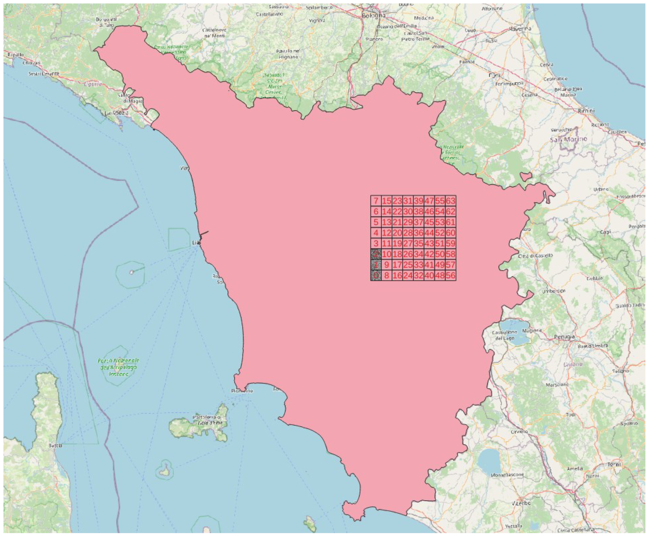
To train the first stage of our pipeline, we used ground truth LC data that are accessible for the territory of Slovenia and can be accessed here [
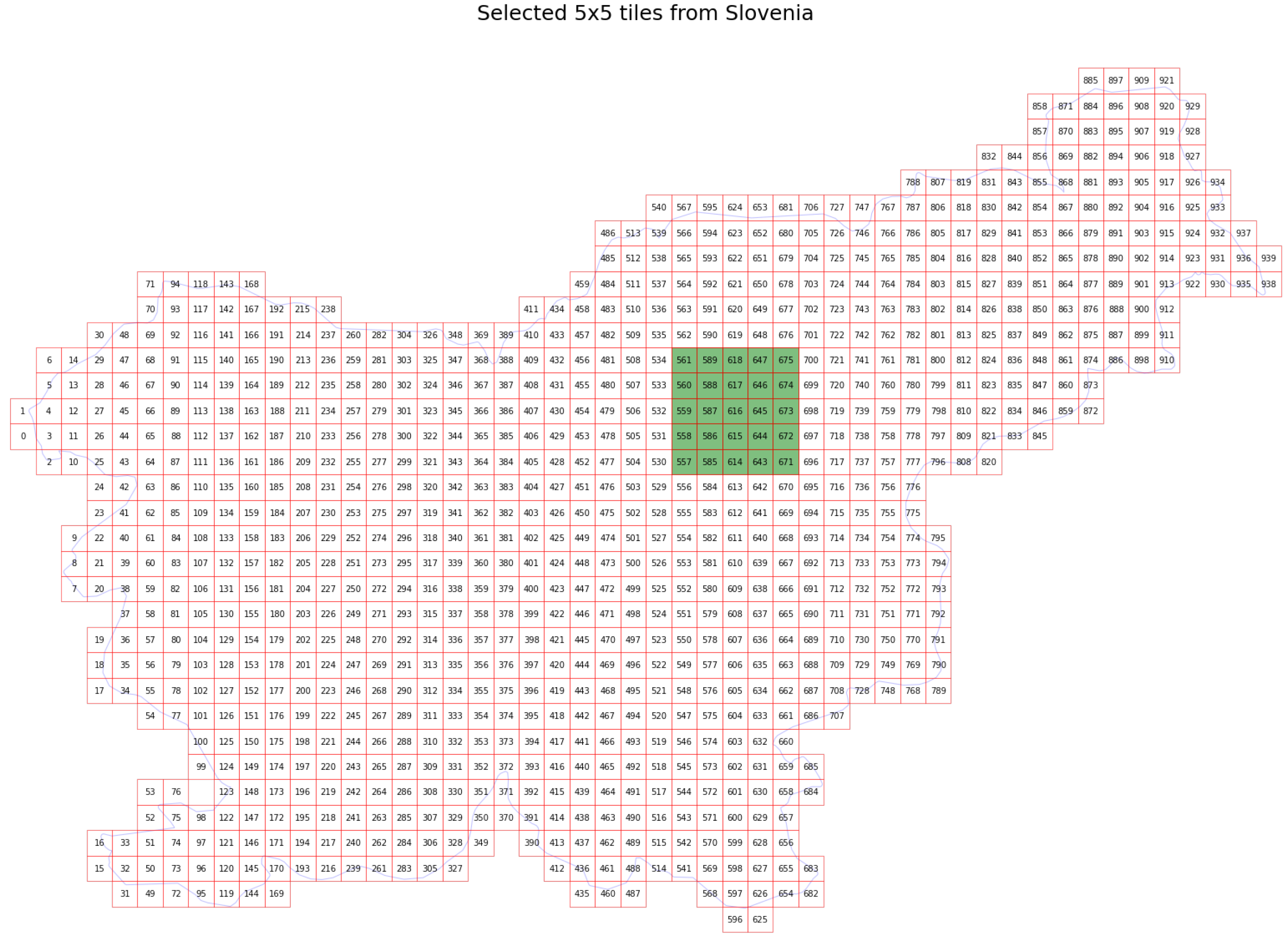
51]. The entire territory of Slovenia is divided into 940 tiles, each sized at 500 × 500 px, with each pixel corresponding to an area of 10 × 10 m
(
Figure 2). The core of the dataset consists of satellite imagery collected by the Sentinel-2 satellites. The country-wide reference for land use/land cover is provided. It is available in the form of a geopackage, which contains polygons and their corresponding labels. The labels represent the following 7 classes:
Although the classes here represented are important for the training of the LULC stage of the model, they were not actually used as the results in our pipeline. It is also worth noting that not all classes have the same representation in the training dataset, which is especially evident if the geography of the region (Slovenia) is taken into account (i.e., mostly mountainous region, with not very many wetlands). It is, therefore, expected that the performance of the segmentation model itself will not be balanced with regard to the reported classes. However, we are only interested in the “knowledge” of the model that gets encapsulated in the latent feature vectors, and do not care too much about the actual classes.
For each tile, general, static, and dynamic data are available. General data include the tile dimensions, geographical coordinates, and timestamps for when the satellite images were captured. Static data encompass information on land cover, categorized into 11 possible classes (cultivated land, forest, grassland, shrubland, water, wetlands, and artificial surface). It is assumed that the land cover either remains stable or changes very little over the one-year interval for which the data were acquired. Dynamic data consist of satellite imagery. Depending on the tile, there were approximately between 50 and 100 satellite images collected during the year 2019. In our training, we used a single image per its corresponding area, selecting those that correspond to the time frame of the existing ground truth LULC map. This time frame is the entire year of 2019; however, we selected the month of July, because it had the least amount of cloud coverage.
3.5. Traversing the Terrain: A Machine Learning Pipeline for Soil Organic Carbon Estimation
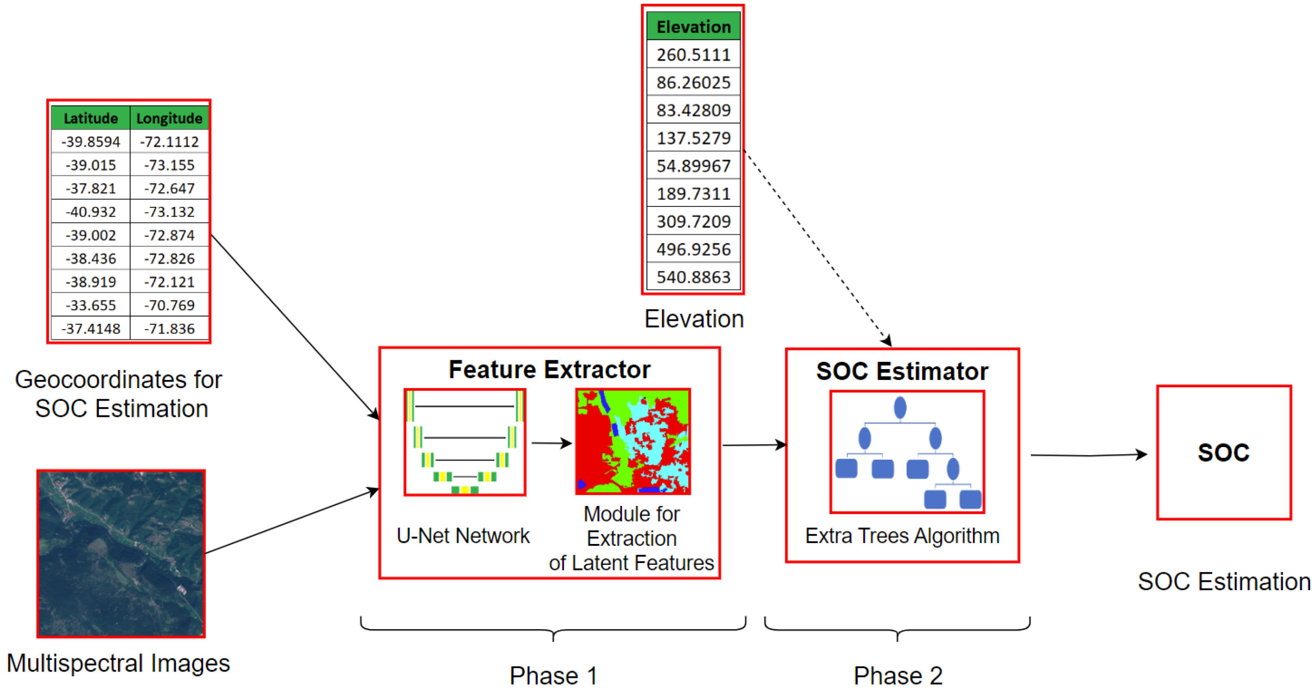
Our machine learning model for SOC estimation consists of two stages, each of which performs a specific function in order to produce the final estimates. The first stage involves training a standard segmentation deep neural network (DNN) with the U-Net architecture. This DNN is trained to estimate the land cover (LC) of an observed region based on multi-spectral images from the Sentinel-2 satellite and a ground truth segmentation map. The trained ANN generates an LC estimation for a region of interest (ROI). This estimation is then used to extract the latent feature vector for each output pixel by rolling back from the output layer of the U-Net and accessing the last available convolutional layer of the same dimension as the output.
The second stage uses the feature vectors extracted at the coordinates for which ground truth SOC measurements exist. Since we are primarily interested in agricultural land and in order for the LUCAS and CHLSOC data to have roughly the same distribution in terms of the type of plots they were sampled at, we retained from the two LUCAS datasets the values for which the observed LC was cropland and grassland.
The pairs of feature vectors and SOC measurements were used to train an independent ML model, which performs the actual SOC estimation. At inference time, the two stages generate a spatially continuous dataset of SOC estimations for patches processed by U-Net. These estimations for different patches are then stitched together to create a map of SOC estimations for an arbitrary geographical region.
In this study, we generated and shared a sample map for the region of Tuscany, Central Italy, with a resolution of 10 m, which is consistent with the highest available resolution of the Sentinel-2 satellite. Tuscany covers about 22,990 km, encompassing a diverse range of terrains including mountains, hills, and coastal plains. Tuscany is world-renowned for its agricultural production. Tuscany’s agricultural sector is celebrated globally for its quality and diversity, from its wine production in Chianti to its olive groves spanning the rolling hills. The region’s fertile soils support a broad range of other crops as well, including grains, legumes, and vegetables, making it a cornerstone of Italy’s food and wine industry. Given the vital role of soil organic carbon (SOC) in maintaining soil fertility and promoting sustainable agricultural practices, Tuscany seemed a good choice to test our model on and provide added value from our research.
3.6. Stage 1—Segmentation DNN for LC Estimation
The focus of our study is the creation of an approach able to generate a map of SOC estimates of the same resolution as that provided by Sentinel-2 imagery, restricted to agricultural applications. However, the amount of training data available for this task is limited, which can hinder the performance of state-of-the-art machine learning models. In addition, the available data sources such as the LUCAS and CHLSOC datasets are sparse, making it impossible to use them for direct end-to-end training of machine learning models for segmentation tasks, which are the basic technology that needs to be used to efficiently address the problem of continuous SOC estimation.
To overcome these limitations, we propose to use transfer learning. We first trained a segmentation network, in our case a U-Net, to accurately predict the LC of a certain geographical location based on Sentinel-2 imagery. Similar to Girschcik et al. [
38], we then extracted the latent features learned by the network to serve as the input to a second-stage ML model to estimate SOC. Since the segmentation network used in the first stage preserves the spatial relations existing in the image, this allowed us to generate spatially continuous predictions of SOC levels for a given region of interest (ROI), taking these relations into account and improving the accuracy of our estimates. A block diagram of the proposed approach is shown in
Figure 3.
To evaluate the performance of the whole pipeline, we used a combination of the CHLSOC and LUCAS 2015 and 2018 datasets and standard metrics: the Mean Absolute Error (MAE), Mean-Squared Error (MSE), Mean Absolute Percentage Error (MAPE), and the coefficient of determination (R2). The latter two provide insight into how large the error is relative to the ground truth value and how much of the variance of the data is explained by the model.
The U-Net Architecture
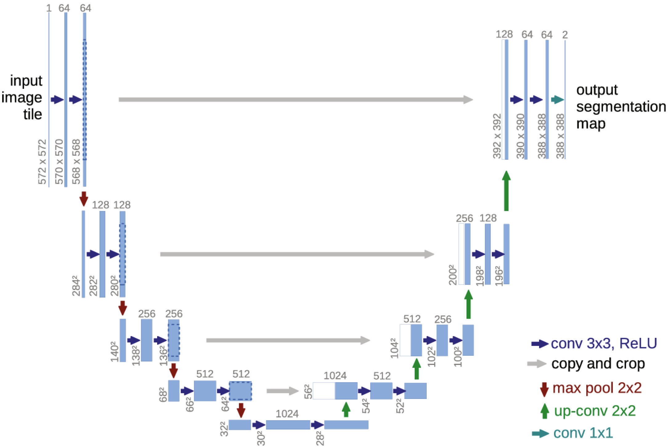
U-Net is a convolutional neural network (CNN) architecture that was developed by Olaf Ronneberger et al. in 2015 at the University of Freiburg in Germany for biomedical image segmentation [
52]. The U-Net architecture is an improvement over the Fully Convolutional Network (FCN) architecture that was developed by Jonathan Long et al. in 2014 [
53]. The architecture is shown in
Figure 4.
The U-Net architecture is composed of two main parts: an encoder and a decoder. The encoder, also known as the contracting path, reduces the spatial dimensions of the input image and increases the number of filters (feature channels) at each of its blocks. This process extracts increasingly abstract and high-level features from the input image. The decoder network, also known as the expansive path, takes the high-level features from the encoder network and uses them to reconstruct a segmentation map of the same size as the input image.
Each encoder block consists of two 3 × 3 px convolutional layers. The activation function of these layers is a Rectified Linear Unit (ReLU), introducing nonlinearity. The output of the ReLU activation function is then passed to the corresponding decoder block using skip connections. This allows the network to retain detailed spatial information in the encoder path and use it to produce more-accurate segmentation maps.
The decoder consists of a sequence of decoder blocks, each of which starts with a 2 × 2 transpose convolutional layer that increases the spatial dimensions of the feature maps. The output of the transpose convolution is then concatenated with the corresponding output of an encoder block passed via the skip connection. This concatenated feature map is then passed through two 3 × 3 convolutional layers with ReLU activation. To produce the final segmentation mask, the output of the last decoder block is passed through a 1 × 1 convolutional layer with sigmoid activation.
To create our LC classifier, we used a U-Net architecture with an input of 64 × 64 px. This provided us with 1436 ground truth LC values across a single dimension of the patch, i.e., more than 2 million training points per patch. The whole EO-learn dataset used for the training and validation of our contains 235 million samples (i.e., Sentinel-2 pixels with LC ground truth labels).
3.7. Stage 2—The SOC Estimator
Once the LC-classifier is trained, one can use the output of any of its layers as features for any transfer learning task related to LC classification. We opted to use the output of the last layer of the network that has the same dimensions as the output of the network, i.e., the first deconvolutional layer of the network (bottleneck), located some 16 layers before the output in our model. Its output is the latent high-level features for each pixel, and we hypothesized that these are relevant for SOC estimation. Each pixel is represented by a vector of 194 values. For a patch, we, therefore, have 794,624 (64 px × 64 px × 194) values.
We, thus, constructed an encoder-only U-Net, which, at inference time, provides us the features for all pixels in the ROI in a single pass.
To create the datasets used to train and evaluate our SOC estimators, Sentinel-2 imagery was downloaded for the the geographical locations for which the SOC ground truth is available. The images downloaded were taken as close as possible to the date of sampling, with the condition that cloud cover was less than 10%. A 64 × 64 px patch is then extracted from these images, centered on each of the locations with the known SOC values and fed into our feature extractor, providing us with a 194-feature vector for each SOC measurement.
This dataset was then used to train and evaluate a number of different machine learning models and approaches listed in
Table 3.
All 13 spectral bands of Sentinel-2 were used in our pipeline. At inference time, the model processes each input image and produces an output of the same 64 × 64 px size. However, to account for the model’s decreasing capacity to maintain context as it approaches the borders of the input image, we discarded a frame 8 px-wide on all sides, resulting in an effective output image size of 48 × 48 px.
To form the final continuous SOC map, we employed a sliding window technique.
4. Experiments and Results
A two-step evaluation procedure was used to account for the specific composition of our pipeline. The first stage of our pipeline was evaluated on the LC classification task, to make sure that the latent features were relevant for the SOC estimation task. Once the performance of the LC classifier was deemed satisfactory, we proceeded with the extraction of latent features for all the relevant samples in the LUCAS and CHLSOC datasets. These then served to evaluate the performance of the whole pipeline.
4.1. LC Classification Performance
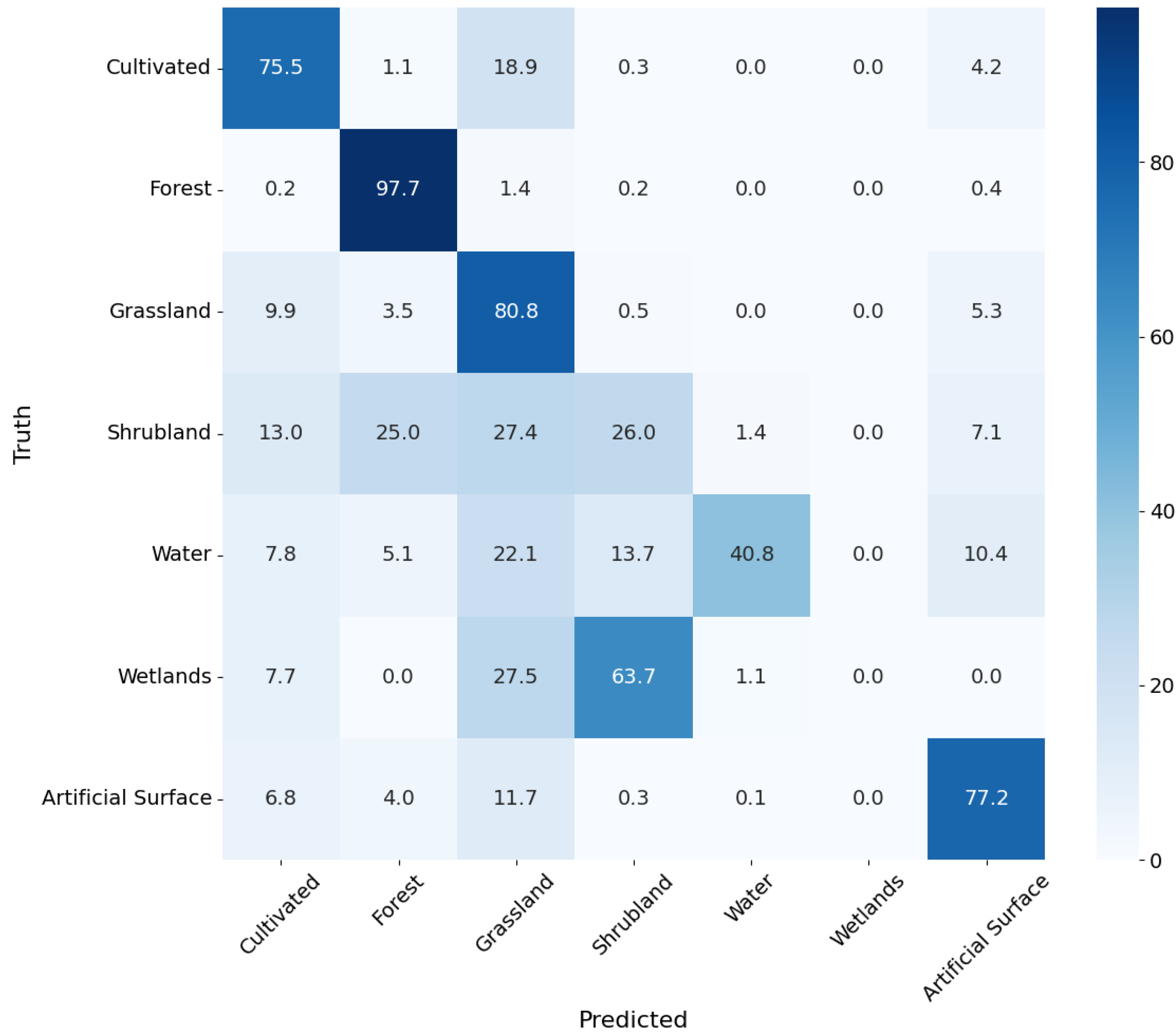
The confusion matrix for our U-Net-based LC classifier is shown in
Figure 5. Seventy percent of the
EO-learn dataset was used for training and the rest for validation. The learning rate used was 0.001, and the batch contained 32 input patches. The model was trained for 100 epochs.
As the confusion matrix, the model was sufficiently accurate for a number of LC classes. The performance was best for forests, which were detected with 97.7% accuracy. Of particular importance for our task were the cultivated land and grassland classes, for which the performance of the model was still good (they were detected with 75.5% and 80.8% accuracy). It is worth noting that, even when the classification for these two classes was wrong, the model tended to confuse these two classes. The only other class that was confused with these two was the artificial surfaces, but these were likely to be an artifact of our training dataset, which contained a portion of artificial surfaces (mainly roads), which were of dimensions smaller than the resolution of Sentinel-2 and could not be reliably identified in the imagery.
The most challenging for the model were the shrubland and wetlands classes. This can be attributed to the relative scarcity of training data pertaining to these surfaces in the dataset. They represented just 0.6% of our dataset.
Since the model was successful in separating the cultivated and grassland classes from the rest of the dataset, we concluded that the latent features extracted will be sufficiently relevant to our ultimate goal.
4.2. SOC Estimates
Using the feature vectors derived from the U-Net encoder, datasets containing the latent features and ground truth SOC values for all samples in CHLSOC and a subset of samples in the LUCAS 2015 and 2018 datasets relevant to our study (i.e., those for which the LC class was cropland and grassland) were constructed. For each entry in the dataset, the geographical coordinates were kept. In addition, we evaluated the impact of adding elevation above sea level to the features, to account for the fact that LUCAS is restricted to lower altitudes and to provide additional information to the model.
Based on these, we evaluated 10 different machine learning algorithms available within the scikit-learn library [
54], aiming to identify the algorithm that exhibited the optimal balance between accuracy and generalization. The candidates included: linear regression, ridge regression, ElasticNet regression, K-Nearest Neighbors regression, extremely randomized trees regression, support vector regression, decision tree regression, random forest regression, gradient boosting regression, and neural network regression.
The models were evaluated using 10-fold cross–validation. The results of these experiments are shown in
Table 3 and
Table 4. As the data in the tables show, adding elevation led to a modest improvement for nearly all of the algorithms tested, except for the MLP, the performance of which deteriorated significantly when elevation was added. Among the algorithms evaluated, extremely randomized trees performed best. We, therefore, decided to conduct further evaluation based on this methodology alone.
4.3. Additional Assessment of Extremely Randomized Trees for SOC Estimation
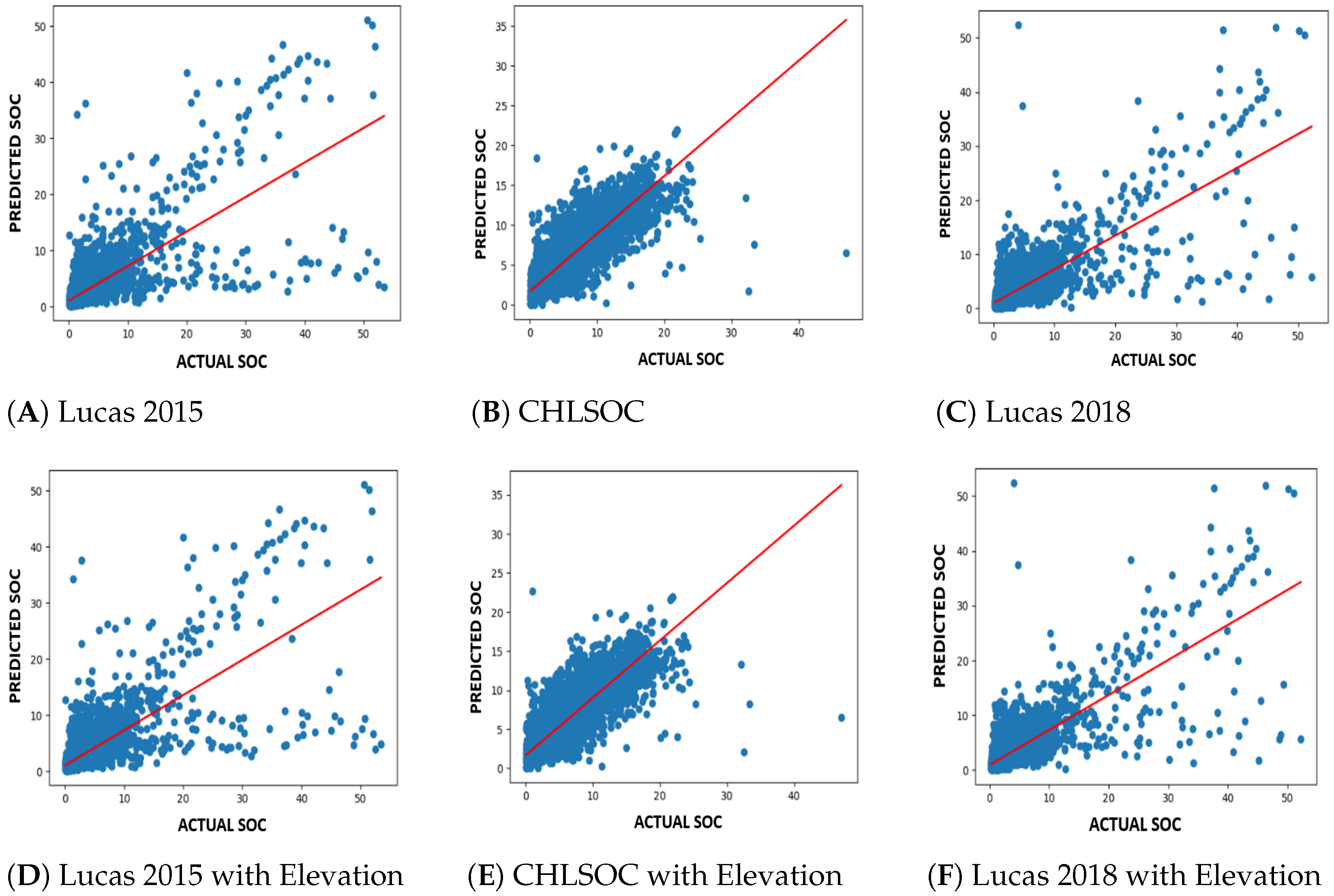
Having settled on extremely randomized trees (ERTs), we attempted to evaluate if the models based on ERTs can generalize across the globe (i.e., CHLSOC and LUCAS datasets). To do so, each fold in our 10-fold cross-validation procedure was created using 100% of two datasets, as well as 90% of the third dataset. The remaining 10% of the third dataset was used for evaluation. Once again, in
Table 5 and
Table 6, we present results with and without elevation. Additionally, in
Figure 6 are represented regression lines for each dataset.
Following the cross-validation, we employed grid search to systematically explore a range of hyper-parameter combinations for the extremely randomized trees algorithm. The objective was to identify the optimal set of hyper-parameters that maximized the R2 score, indicating the goodness-of-fit of the model. The search spanned various values for key parameters, including the number of trees in the forest (n estimators), the maximum number of features considered for splitting a node (max features), the minimum number of samples required to be at a leaf node (min samples leaf), the minimum number of samples required to split an internal node (min samples split), and the seed for the random number generator (random state).
The parameter ranges are defined as follows: n estimators ranged from 100 to 200 in increments of 25; max features ranged from 91 to 130 in increments of 10; min samples leaf ranged from 1 to 9 in increments of 2; min samples split ranged from 2 to 8 in increments of 2; the random state ranged from 0 to 4 in increments of 2.
After the grid search, the optimal combination of the hyper-parameters for the extremely randomized trees model was identified as follows: “n estimators” set to 100, “max features” set to 121, “min samples leaf” set to 1, “min samples split” set to 2, and “random state” set to 4.
Once the map was generated, we used the CORINE dataset to create a validity mask for our SOC map.
4.4. Constructing the SOC Map: Application of the Model and Mosaicking Approach
In the final stage of our pipeline, we used our mosaicking approach to produce a continuous, high-resolution SOC map.
Each input image fed to the first stage of our pipeline was 64 × 64 px, with each pixel representing a 10 × 10 m area on the ground. All 13 spectral bands of Sentinel-2 were used. The model processes each input image and produces an output of the same 64 × 64 px size. However, each output image is padded by 8 px on all sides, resulting in an valid output image size of 48 × 48 px. This padding strategy was employed to account for the model’s decreasing capacity to maintain context as it approaches the borders of the input image.
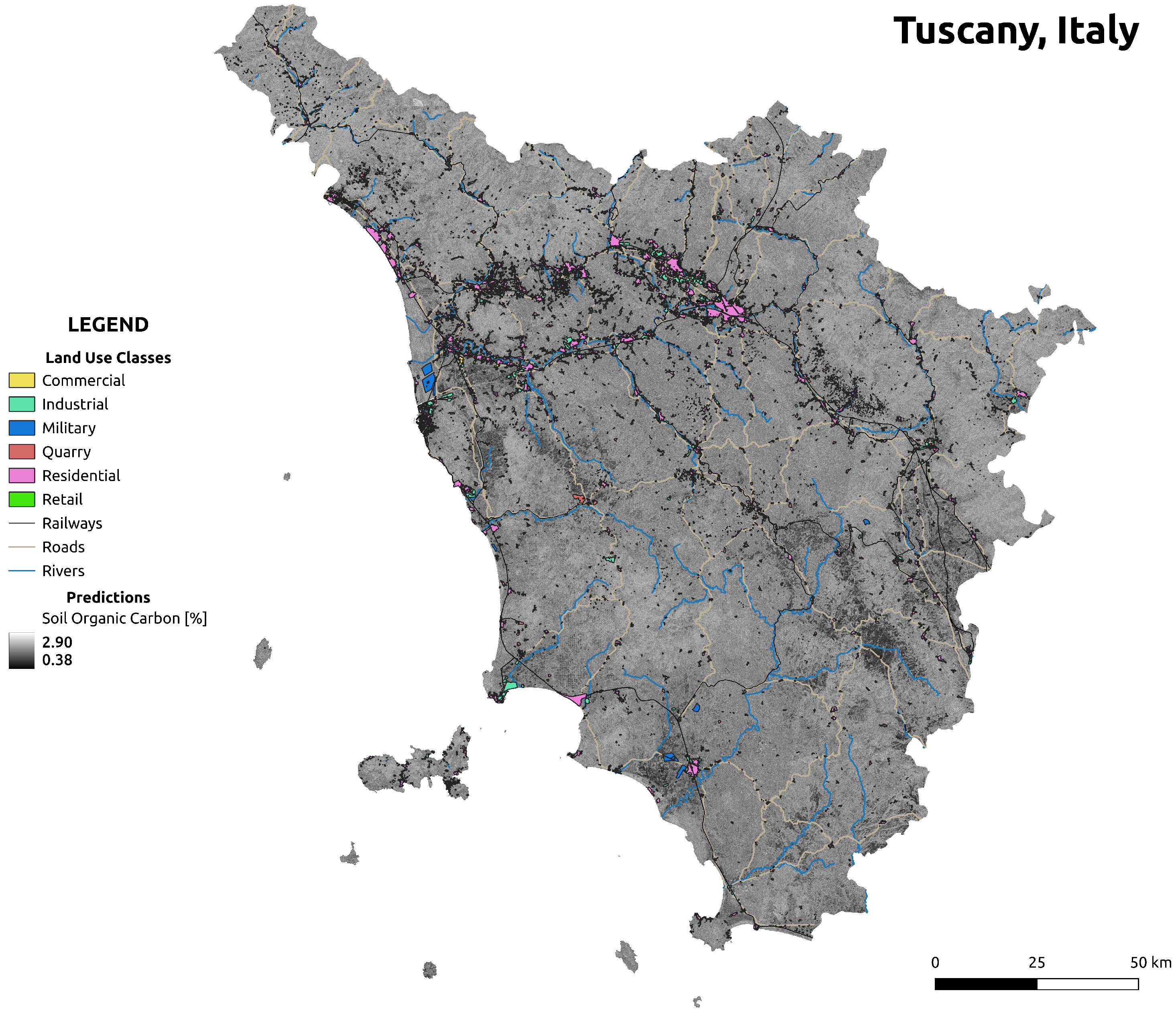
To form the final continuous SOC map, we employed a sliding window technique. This technique ensures that the 48 × 48 px output images (tiles) are perfectly adjacent to each other, resulting in a seamless, continuous map, shown in
Figure 7. The application of this technique requires careful consideration of the input image dimensions, output image dimensions, and padding to ensure accurate alignment and continuity of the final SOC map. By employing this methodology, we were able to leverage the predictive power of our model across the landscape, generating an accurate, high-resolution, and continuous representation of SOC content across Tuscany.
Once the map was generated, we used the CORINE dataset to create a validity mask for our SOC map.
In particular, CLC2018 was used, the publicly available and up-to-date version of CORINE. The CLC2018 data were used in their native raster format, to eliminate SOC estimates for land cover classes that our model was not trained for. We restricted our estimates to categories 2 and 3, as shown in
Table 7 (Agricultural areas and Forest and semi-natural areas), as regions of interest within the study area, while everything else was considered as an area with invalid data. The result is a raster layer of data that clearly separates cultivated areas and areas under vegetation from built-up areas and areas under water.
Product Generation and Availability
In the execution of our methodology, we successfully generated a high-resolution, continuous soil organic carbon (SOC) map for the region of Tuscany.
The SOC map, alongside the CORINE-based validity mask, provides a valuable resource for understanding SOC distribution relative to different land use and land cover classes. These products, formatted as GeoTIFF files, can be easily integrated into further spatial analyses.
To facilitate the use of these data products, we provide Python examples demonstrating how to interact with these files in our GitHub repositories. These repositories contain not only the data, but also detailed guidance for engaging with the data using popular geospatial Python libraries.
To visually grasp the SOC distribution across Tuscany, please refer to
Figure 8. This figure, entitled “Grayscale representation of SOC values with validity overlay”, illustrates SOC content across the region with an overlay of the validity mask.
The tools and data we generated promise to support future research endeavors and inform sustainable management practices in Tuscany’s rich agricultural landscapes. For this purpose, we share our code at
https://github.com/iai-rs/soc (accessed on 4 January 2024).
5. Discussion
5.1. Comparison and Validation of Results
While remote sensing is the most-promising methodology in terms of achieving affordable and global SOC monitoring, the studies focusing solely on satellite imagery have been limited in scope (i.e., the number of soil samples used to develop and validate the models and the area covered).
Table 8 shows the comparison between our results and other relevant approaches published in the literature. It should be noted that the highest R
2 was obtained by Steinberg et al., but it relies on hyperspectral data and is limited to just 81 ground truth sample taken over an area just 7 km
, making it very hard to judge how general this measure of performance is.
Similarly, the recent approach proposed by Castaldi et al. limits the models to specific areas, ranging between 2.2 and 425 ha, so the question of how their approach could be scaled to global- or continent-level SOC monitoring remains unanswered.
The proposed approach, however, nearly matches the performance of Steinberg et al. on CHLSOC, which covers an area more than 100,000-times larger in size and contains 85-times more data than were used by Steinberg et al., making the evaluation performed in the study presented here much more extensive. Of the previous studies, the closest in size in terms of the number of samples is that of Emadi et al., but their dataset is still several orders of magnitude smaller and the study was restricted to Northern Iran. However, when evaluated on our entire dataset comprised on CHLSOC, LUCAS 2015, and LUCAS 2018, we were very near the performance achieved by Emadi et al. in terms of the variance explained by our model (R). A valid comparison in terms of the RMSE is virtually impossible to achieve, since the range of SOC in different studies varies drastically.
In
Table 6, we show the MAPE as a measure of the performance of our approach as well. This allowed us to conclude that, on average, our model missed the SOC value by 48.6%. While this certainly is a large margin of error, it is also a significant improvement when one takes into account that the current global estimates of SOC vary between 504 and 3000 Pg C [
16].
5.2. Research Limitations
While this study has produced meaningful results, it is important to acknowledge its limitations.
The main limitation is that we restricted our training data to a subset of land cover classes available in LUCAS. While we did not perform any filtering on the dataset, our model best performed on CHLSOC, and it is also restricted to a subset of land covers by design. The majority of data points were concentrated in specific regions, such as deciduous forests, broad-leaved forests, sclerophyllous forests, and thorny forests. These areas, characterized by high-quality soil and available water, have experienced significant land use conversion, making them of particular interest to our study. On the other hand, certain regions, such as the high Andes, the Atacama Desert, and western Patagonia, are underrepresented in terms of soil data. The lack of comprehensive data in these ecologically significant regions restricts our understanding of soil organic carbon dynamics and ecosystem processes in these areas, as well as the applicability of our model.
This is why we chose to use CORINE to filter our predictions of our model that cannot reasonably be expected to be valid. But, to create an approach able to monitor the SOC across all ecosystems, further data need to be collected and integrated into the proposed approach.
An additional limitation of our approach is that we did not consider the temporal dynamics of SOC and that the model predicts the value based on a single satellite image. This is a limitation that we aim to address in the near future.
6. Conclusions
Monitoring soil organic carbon (SOC) typically assumes conducting a labor-intensive soil sampling campaign, followed by laboratory testing, which is both expensive and impractical for generating useful, spatially continuous data products.
In the study presented, we proposed a hybrid approach to estimate SOC remotely from Sentinel-2 satellite imagery. The approach relies on a novel two-stage pipeline, using a DNN (U-Net) trained to classify land cover to perform feature extraction and a different ML model to perform the SOC estimation.
The proposed approach was evaluated on the largest dataset publicly available today, constructed of CHILSOC and LUCAS, and achieved results comparable to previous studies evaluated on several datasets that are orders of magnitude smaller and geographical regions, making it the first approach with the potential to scale to global SOC estimation and monitoring.
To demonstrate the usability of the proposed approach, we generated and shared a high-resolution map of SOC for the Italian region of Tuscany, in an effort to enable external validation of the methodology, as well as to stimulate the development of possible applications based on approaches such as the one presented in this paper.
The work serves as a significant step toward implementing efficient, cost-effective, and remote SOC monitoring on a global scale. The demonstrated integration of satellite imagery and machine learning in SOC estimation opens a promising avenue for further research and practical applications, particularly in environmental science and land management.


 ,
, 
