Hyperspectral Reconstruction Method Based on Global Gradient Information and Local Low-Rank Priors

Abstract

Hyperspectral compressed imaging is a novel imaging detection technology based on compressed sensing theory that can quickly acquire spectral information of terrestrial objects in a single exposure. It combines reconstruction algorithms to recover hyperspectral data from low-dimensional measurement images. However, hyperspectral images from different scenes often exhibit high-frequency data sparsity and existing deep reconstruction algorithms struggle to establish accurate mapping models, leading to issues with detail loss in the reconstruction results. To address this issue, we propose a hyperspectral reconstruction method based on global gradient information and local low-rank priors. First, to improve the prior model’s efficiency in utilizing information of different frequencies, we design a gradient sampling strategy and training framework based on decision trees, leveraging changes in the loss function gradient information to enhance the model’s predictive capability for data of varying frequencies. Second, utilizing the local low-rank prior characteristics of the representative coefficient matrix, we develop a sparse sensing denoising module to effectively improve the local smoothness of point predictions. Finally, by establishing a regularization term for the reconstruction process based on the semantic similarity between the denoised results and prior spectral data, we ensure spatial consistency and spectral fidelity in the reconstruction results. Experimental results indicate that the proposed method achieves better detail recovery across different scenes, demonstrates improved generalization performance for reconstructing information of various frequencies, and yields higher reconstruction quality.

1. Introduction

Hyperspectral remote sensing images are obtained by hyperspectral imaging devices that capture images of targets across different spectral bands, allowing for the simultaneous acquisition of rich spatial and spectral information about the target objects [1]. By analyzing the differences in spatial spectral features of the target objects at various wavelengths, the reliability of quantitative analysis can be significantly enhanced, making this technology broadly applicable in fields such as remote sensing [2], mineral exploration [3], agricultural monitoring [4], and ecological environment monitoring [5].

Depending on the acquisition method, hyperspectral imaging devices can be classified into four types: point scanning, line scanning, spectral scanning, and snapshot hyperspectral imaging. Typically, these devices require point-by-point or line-by-line scanning at different wavelengths to obtain complete spatial spectral information, resulting in long acquisition times and difficulties in rapidly capturing dynamic targets [6]. Snapshot hyperspectral imaging faces challenges in simultaneously meeting demand in terms of both spatial and spectral resolution. However, the snapshot compressed spectral imaging technology [7] enables rapid collection of hyperspectral data, yielding high-quality results when combined with reconstruction algorithms. Compared to traditional hyperspectral remote sensing imaging systems, this method offers higher acquisition efficiency and provides more accurate and effective data processing methods for future Earth observation, environmental monitoring, and geospatial analysis. Represented by coded aperture snapshot compressed spectral imaging systems [8], this approach utilizes spatial spectral modulation through coded apertures and dispersive elements, allowing the receiver to obtain full-band measurement images with only a two-dimensional image sensor. Compared to traditional hyperspectral remote sensing imaging devices, it features a simpler hardware design and higher acquisition efficiency, providing a new way to rapidly collect hyperspectral remote sensing information.

However, the process of reconstructing high-dimensional spectral images from low-dimensional compressed measurement images is an underdetermined problem [9]. Traditional reconstruction methods often utilize the statistical properties, spatial correlations, and spectral characteristics of the spectral images as regularization terms in the solving process. By constraining the solution space, these methods help to achieve a reconstruction result that is closer to the true image [10]. However, traditional regularization methods often fail to accurately reflect the complex structural information of images with highly variable texture during reconstruction, leading to discontinuous edges or distortion in the results. To reduce the dependence on general priors in the reconstruction process, deep learning algorithms leverage deep networks to fit the probability distribution of prior data, realizing a nonlinear mapping from low-dimensional measurements to high-dimensional spectral images [11]. Common deep learning reconstruction algorithm frameworks are mainly categorized into four types: end-to-end neural networks, deep unfolding, plug-and-play (PnP) methods, and deep image prior-based compressive spectral reconstruction algorithms. Network structures based on end-to-end and deep image prior reconstruction algorithms can be divided into convolutional neural network-based structures [12], attention mechanism-fused structures [13], and self-attention mechanism-based transformer structures [14]. However, deep network models typically use fixed convolution kernels, which makes their static feature extraction strategies insufficient for capturing dynamic changes in complex backgrounds. Introducing attention mechanisms can enhance the adaptability of deep network models; however, as the number of convolutional layers increases, the problem of high-frequency feature gradient vanishing arises, making it easier for the network model to lose high-frequency information when reconstructing local details.

To address the above issues, we propose a compressed spectral reconstruction method based on global gradient information and local low-rank priors. First, we perform equal-width binning on the input features to accurately separate high-frequency and low-frequency information, training the model on each discrete interval to accelerate the training efficiency. Second, to enhance the model’s sensitivity to different frequency information, we sort and resample features based on the magnitude of the loss function gradient during training, applying a higher sampling ratio for large-gradient samples and random sampling for small-gradient samples. This further improves the prior model’s training efficiency with respect to different frequency information. Additionally, to mitigate potential smoothness issues arising from point predictions, we design a sparse sensing denoising module with local smoothness constraints, utilizing the smooth low-rank nature of the representation coefficient matrix after singular value decomposition to enhance the smoothness of pixel neighborhoods in the prediction results. Finally, based on the semantic similarity between the denoised results and the original spectral image, we reformulate the reconstruction problem as a total variation (TV) minimization problem between the denoised results and the reconstructed results, implementing an optimized solution for compressed spectral imaging using the alternating direction method of multipliers (ADMM).

The main contributions of the proposed hyperspectral reconstruction method based on the global gradient and local low-rank priors can be summarized as follows:

(1) A new gradient-boosted reconstruction framework that discretizes continuous numerical features into a finite number of interval representations. By combining a gradient-boosting sampling strategy, the training weights for high-gradient samples are increased during the training process, effectively improving the prior model’s predictive performance on prior data and allowing the predictions to better preserve high-frequency detail information.

(2) Utilizing the local low-rank characteristics of the representative coefficient matrix, we design a sparse sensing denoising module based on singular value decomposition. This approach enhances the local smoothness of neighboring pixels while maintaining the global structural information of the predictions, further strengthening the regularization constraints in the reconstruction process.

(3) By leveraging the semantic similarity between the denoised results and prior spectral data, we transform the reconstruction problem into a total variation minimization problem between the denoised results and the reconstructed spectral data. This provides better guidance for hyperspectral reconstruction solutions. Experiments across various scenes demonstrate that the proposed method more effectively preserves image edges and detail information, resulting in superior reconstruction quality.

2. Materials and Methods

2.1. Related Work

In this section, we primarily review the principles of hyperspectral image compressed sensing and related reconstruction algorithms, then analyze and summarize the limitations of existing reconstruction methods.

2.1.1. Hyperspectral Compressed Sensing Process

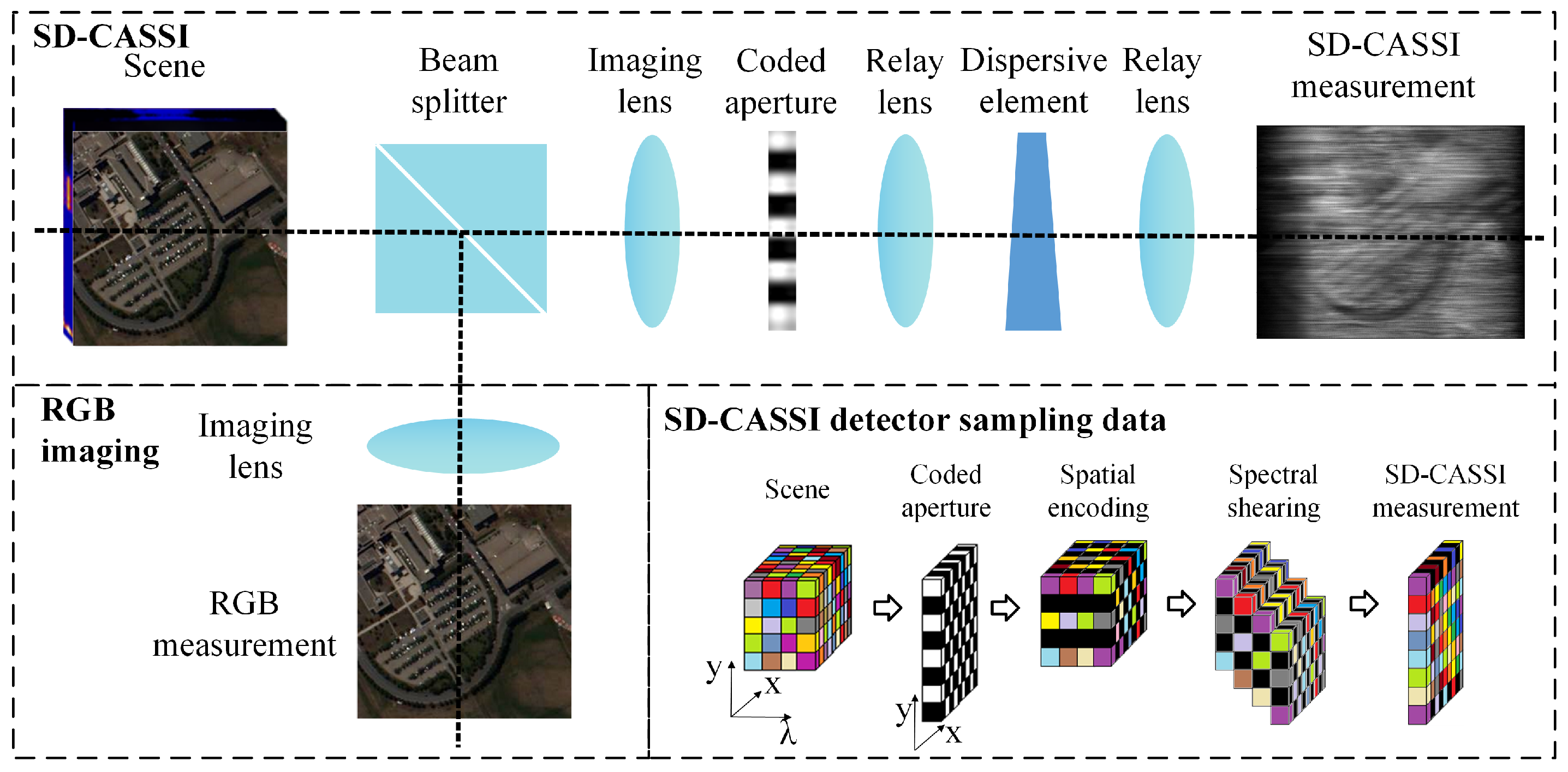
The first hyperspectral compressed sensing system was proposed by Duke University [15]. In this system, incident light passes through spatial modulation and spectral modulation before being compressed onto a two-dimensional (2D) detector. Spatial modulation is achieved using a 2D coded aperture, while spectral modulation is primarily performed using dispersive elements or diffraction gratings. However, improving the quality of reconstructing low-dimensional measurement images into high-dimensional spectral information often requires more stringent constraints. To enhance reconstruction quality, researchers have incorporated an additional unencoded grayscale imaging or RGB imaging channel through dispersive elements to supplement the reconstruction process [16]. As shown in Figure 1, the incident light first encounters a beamsplitter, where one path leads to the snapshot compressed spectral imaging (CSI) system after spatial and spectral modulation; this is superimposed onto the 2D detector, while the other path is captured by the unencoded RGB imaging system.

Figure 1. Structural composition of the DCCHI system and data structure of SD-CASSI detector sampling.

The forward model of SD-CASSI is linear [17], and the spatial resolution of the coded aperture M determines the spatial resolution of the entire imaging system. When a 3D spectral data cube $x^{h\times w\times c}$ with c spectral channels passes through the coded aperture, each band is multiplied by M to obtain the modulation result:

$$x^{\prime }(:,:,\lambda )=x(:,:,\lambda )\odot M$$

(1)

where $x^{\prime }(:,:,\lambda )$ represents the spectral image of the $\lambda$-th band after modulation, ⊙ represents the element-wise tensor multiplication, and $x(:,:,\lambda )$ represents the image of the $\lambda$-th $(1\le \lambda \le c)$ band. Assuming that the dispersion direction is the w direction and the relative displacement of adjacent bands is d, the dispersed spectral data is

$$x^{″}(u,v,{\lambda }_b)=x^{\prime }(h,w+d\times ({\lambda }_b-{\lambda }_c),{\lambda }_b),$$

(2)

where $x^{″}(u,v,{\lambda }_b)$ represents the data translated by $d\times (c-1)$ columns in the w direction, $(u,v)$ represents the coordinate of the sensor plane, ${\lambda }_b$ represents the b-th spectral band, and ${\lambda }_c$ represents the reference fixed band. Finally, the 2D compressed measurement image y is obtained by superimposing the spectral dimension on the sensor plane:

$$y=\sum _{b=1}^c{x}^{″}(u,v,{\lambda }_b).$$

(3)

The RGB imaging detection process can be expressed as follows:

$$y_{rgb}=S_{rgb}\odot x(u,v,{\lambda }_b)$$

(4)

where $y_{rgb}$ represents the RGB image and $S_{rgb}$ denotes the sensing matrix of the RGB imaging pathway.

2.1.2. Existing Reconstruction Algorithms and Their Limitations

Existing CASSI reconstruction algorithms are mainly divided into convex optimization reconstruction algorithms with sparse priors and deep learning-based reconstruction algorithm models [18]. Convex optimization algorithms model the reconstruction process as an optimization problem of the objective function, using methods such as gradient descent and conjugate gradient methods to iteratively find the optimal solution by minimizing the objective function. Common optimization methods include the Two-step Iterative Shrinkage–Thresholding Algorithm (TwIST) [19], the Split Bregman algorithm [20], the ADMM [21], and the Generalized Alternating Projection (GAP) method [22]. To reduce the solution space and improve accuracy, regularization terms are typically introduced in the objective function based on the smoothness, sparsity, and low rank of the spectral image to constrain the characteristics of the reconstructed image. The TV model measures the local smoothness of the image information by minimizing the gradients in the horizontal and vertical directions through total variation regularization; in this way, the reconstruction results can exhibit more smoothing characteristics [23]. However, manually designed regularization terms make it challenging to obtain a solution model that closely approximates the original data distribution. Consequently, the reconstruction quality of traditional convex optimization algorithms is not high and they require multiple iterations, leading to long reconstruction times.

Deep learning algorithms have high learning efficiency [24]. By introducing deep networks into the reconstruction process, these algorithms can fit the prior spectral data distribution through network models, achieving nonlinear mapping from low-dimensional to high-dimensional spaces. This replaces the multiple constraints of traditional algorithms with the model’s loss function, effectively simplifying the issues of high computational complexity and long reconstruction times associated with convex optimization reconstruction algorithms. For example, during the training process of an end-to-end neural network model, measurement images and coding aperture matrices are used as input features, with the true values as the target. The training focuses on the nonlinear mapping relationship between the measurement images and the true values. Deep unfolding networks combine traditional optimization algorithms with neural networks, unfolding iterative algorithms into multiple stages of cascading subnetworks. This approach uses neural networks to replace the constraints of prior terms, allowing each subnetwork to focus on different levels of denoising tasks, thereby enhancing the overall performance of the network. However, the cascading of multistage subnetworks can deepen the network structure, leading to an increase in model parameters and a higher risk of overfitting during the training process. The PnP algorithm [25] employs a pretrained model as a prior in the optimization algorithm, using proximal gradient methods and image denoising networks for iterative reconstruction. Common proximal gradient algorithms include gradient descent [26], half-quadratic splitting [27], and Douglas–Rachford splitting [28]. However, the reconstruction process requires hundreds of iterations, resulting in longer reconstruction times.

An accurate regularization term can accelerate convergence speed and improve reconstruction quality. Chen et al. [29] used RGB images or grayscale images as a supplement during the reconstruction process, establishing a regularization term based on the semantic similarity between the interpolation results of RGB images and the original images. By combining this with convex optimization algorithms, they achieved a final optimization solution with enhanced reconstruction quality; however, this approach is not applicable to the near-infrared portion beyond visible light. Utilizing deep learning methods, a prior model can be trained with RGB images or grayscale images, with the semantic similarity of the prior model’s predictions established as a regularization term. This allows the reconstruction model to achieve more generalized reconstruction performance. However, the structural design of the prior network can easily lead to gradient vanishing issues for deep features, which is detrimental to the refined representation of high-frequency information and may result in the loss of detailed texture information.

2.2. Methods

2.2.1. Overall Architecture

Figure 2 illustrates the framework of the proposed algorithm for the compressed spectral reconstruction method based on global gradient information and local low-rank priors. First, global feature extraction is performed on the RGB image to identify the optimal split points for prior model establishment. Next, the prior model establishment process employs a gradient boosting training strategy, optimizing feature selection using the gradient information from the loss function. This enables the model to better focus on high-frequency data with larger errors, while dimensionality reduction along the channel dimension is achieved through exclusive feature bundling to enhance training efficiency. The sparse sensing reconstruction model is composed of a prior degraded sensing model and a CSI reconstruction model. A local smooth prior representing the coefficients is designed to form a sparse sensing denoising model, improving the local smoothness of the prior model’s predictions. The difference between the denoised result and the reconstruction result establishes a regularization constraint for the reconstruction process, which is optimized using the ADMM algorithm to achieve the final solution.

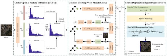
Figure 2. Reconstruction algorithm framework.

2.2.2. Determination of the Global Optimal Split Points

To address the challenge of accurately capturing key features during training with a large volume of pixel data, the input features are discretized into different frequency intervals. By utilizing statistical information for rapid node splitting, this approach significantly enhances the model’s efficiency in utilizing different frequency information while reducing computational complexity. Specifically, for three-channel RGB images, the intensity values of each color channel are uniformly divided into K discrete intervals ranging from 0 to 255; this division converts continuous color intensity values into a series of ordered interval representations, with each interval corresponding to a unique index value ranging from 0 to K. The belongingness interval is determined by traversing each pixel in the three channels, then the color value of the pixel in that channel is replaced with the corresponding interval index. This feature processing method retains the basic distribution characteristics of different frequency information, providing an efficient representation for model training.

When constructing the prior model, a regression tree model is built using discrete intervals as the splitting nodes. By comparing the prediction errors before and after the split of each node, the feature that can minimize the global error to the greatest extent is selected as the current node to initialize the prior model. The calculation formulas for the loss before split ($LBS$) of the current node, local loss of the left split node $L_{R1}$, reduction in local loss ($RLL$), local loss of the right split node $L_{R2}$, and reduction in global loss ($RGL$) can be expressed as follows:

$$LBS={\displaystyle \frac{{\sum }_{i\in R_C}{(y_{(C,i)}-{\widehat{y}}_{(C,i)})}^2}{n}}$$

(5)

$$L_{R_1}={\displaystyle \frac{{\sum }_{i\in R_1(C,m)}{(y_{(C,i)}-{\widehat{y}}_{(C,R_1,i)})}^2}{n_{R_1}}}$$

(6)

$$L_{R_2}={\displaystyle \frac{{\sum }_{i\in R_2(C,m)}{(y_{(C,i)}-{\widehat{y}}_{(C,R_2,i)})}^2}{n_{R_2}}}$$

(7)

$$RLL=\underset{bin\in (0,K)}{max}(LBS-L_{R_1}-L_{R_2})$$

(8)

$$RGL=max\sum _{C\in (R,G,B)}\sum _{bin=0}^{K}RLL$$

(9)

where C represents the three color channels of an RGB image, m denotes the current node, i represents the i-th feature data index at node m in color channel c, $y_{(C,i)}$ and ${\widehat{y}}_{(C,i)}$ respectively represent the original data and the model’s predicted results at channel c and index i before the split at node m, $R_1$ is the data space of the left node after the split and $R_2$ the data space of the right node (where $R=R_1\cup R_2$), ${\widehat{y}}_{(C,R_1,i)}$ and ${\widehat{y}}_{(C,R_2,i)}$ represent the predicted results of the left and right subtree models, respectively, after the split at node m, and $bin$ is the index of the discrete interval corresponding to the current splitting node. When $RLL$ is positive, it indicates that the splitting node helps to reduce the prediction error, when $RLL$ is zero, it indicates that there is no change in the prediction error before and after the split, and when $RLL$ is negative, it indicates that the splitting node increases the prediction error.

2.2.3. Gradient Boosting Prior Model (GBM)

In machine learning algorithms, the loss function reflects the difference between the model’s predicted values and the true values [30]. The training process of the model typically aims to minimize the loss function to achieve a good fit for the training data. Calculating the gradient of the loss function can indicate the training direction of the model parameters, guiding updates to these parameters. To further enhance the efficiency of the prior model in utilizing information from different frequencies, we employed a one-sided gradient boosting sampling algorithm to optimize the data during the training process. Samples are selected based on the magnitude of the loss function gradient, where samples with larger gradients have a more significant impact on adjusting the training of the model parameters. By retaining large gradient samples while randomly sampling from those with smaller gradients and introducing a weighting factor to correct the distribution bias caused by one-sided random sampling, we aim to avoid the issue of the model becoming overly reliant on large gradient samples, which can lead to overfitting.

During the model training process, we take the MSE as the loss function; by calculating the negative gradient of the loss function, we reflect the training direction of the model. The absolute value of the loss function gradient is represented by the symbol $g_t$. In each iteration of the training process, sorting is performed in descending order according to the absolute value of the gradient, with the top $a\times 100\%$ selected as the large-gradient sample data A. We then randomly sample $b\times 100\%$ of the remaining part with a smaller absolute value of the gradient as the small-gradient sample B, establishing a new generation of feature data $A\cup B$. At the same time, to reduce redundant information and simplify the feature representation, we adopt the mutually exclusive feature bundling operation, retain one of the overlapping features, and add the non-overlapping features to form a new composite feature. This reduces the dimension of the features without losing their ability to represent information, and also improves the calculation efficiency of the algorithm. Finally, to discretize the next generation of feature data, the optimal split points for the new model are determined by maximizing the variance gain for each discrete interval. The formula for calculating variance gain can be expressed as follows:

$$H_j\left(m\right)={\displaystyle \frac{1}{n}}[{\displaystyle \frac{{\displaystyle \sum _{t\in A_l}}{g}_t+\frac{1-a}{b}{\displaystyle \sum _{t\in B_l}}{g}_t}{n_l^j\left(m\right)}}+{\displaystyle \frac{{\displaystyle \sum _{t\in A_r}}{g}_t+\frac{1-a}{b}{\displaystyle \sum _{t\in B_r}}{g}_t}{n_r^j\left(m\right)}}]$$

(10)

where j is the feature attribute of the node, t is the variable for the number of features, $g_t$ is the absolute value of the gradient of the loss function, $A_l$ and $B_l$ are the value spaces when the feature value is less than m, $A_r$ and $B_r$ are the value spaces when the feature value is greater than m, ${\displaystyle \frac{1-a}{b}}$ is the normalization coefficient, which normalizes the sum of the gradients of the small-gradient sample B to the size of A, and $n_l$ and $n_r$ respectively represent the number of features less than m and the number of features greater than m.

2.2.4. Degradation-Aware Reconstruction Model

To enhance the local smoothness of the prior model’s prediction results, we first use singular value decomposition to decompose the prediction results into a form that represents the product of a coefficient matrix and basis vectors. The coefficient matrix contains the main structural information of the prediction results and exhibits good local low-rank smoothness, with each element representing the weight of the corresponding basis vector [31]. By utilizing the low-rank smoothness of the first and second derivatives of the coefficient matrix, we establish a sparse denoising model (SDM). To reduce fluctuations in the prediction results within the pixel neighborhood, a soft-thresholding function is introduced to impose local smoothing constraints on the gradient of the coefficient matrix, thereby controlling the issue of large gradients in the neighborhood pixel regions. The definition of the soft thresholding constraint function [32] can be expressed as follows:

$$S\left(x\right)=sign\left({\nabla }_t\left(U\right)\right)•max(\mid {\nabla }_t\left(U\right)\mid -\omega ,0)$$

(11)

$$s.t.\omega ={\displaystyle \frac{max(\mid {\nabla }_t\left(U\right)\mid )}{2}},t=1,2$$

(12)

where U represents the coefficient matrix obtained from the singular value decomposition $x_{gbm}$, ${\nabla }_t\left(U\right)$ represents the gradient of the representative coefficient matrix U, and $\omega$ is the threshold parameter, for which the magnitude is set to 0 for regions with absolute gradient values less than $\omega$ while retaining regions with larger gradients; when $t=1$, it is the first-order derivative, reflecting the change of U between different bands, while when $t=2$ it is the second-order derivative, reflecting the curvature of the change of U between different bands. The process of denoising the coefficient representation can be described as follows:

$$\widehat{U},\widehat{V}=\underset{U,V}{min}\sum _{t=1}^2{\tau }_t \Vert {\nabla }_t{\left(U\right) \Vert }_2+{\Vert V{V}^{\top }-I \Vert }_2$$

(13)

$$s.t.\left\{\begin{array}{c}\hfill x_{gbm}=SVD\left(x_{gbm}\right)+E\hfill \\ \hfill SVD\left(x_{gbm}\right)=U{V}^{\top }\hfill \end{array}\right.$$

where $SVD\left(x_{gbm}\right)$ represents the $SVD$ decomposition of the prior model prediction result $x_{gbm}$, V represents the orthogonal basis vector, E represents the influence of the fluctuation error or noise on the result generated by the prior model prediction result, ${\tau }_t$ represents the weight balance factor, I is the identity matrix, and $\widehat{U}$ and $\widehat{V}$ are the variables to be optimized.

In the SD-CASSI reconstruction process, a regularization term is typically introduced into the objective function to narrow the solution space and improve the stability and accuracy of the solution. The output of the SDM has higher visual similarity to the prior spectral image in terms of semantic aspects such as visual objects, colors, and textures. By establishing a regularization term for the reconstruction process based on the higher semantic similarity between the denoised result and the original image, the reconstruction problem can be more precisely constrained, transforming the reconstruction optimization problem into the problem of minimizing the difference in total variation between the denoised result and the reconstructed spectral data. The objective function for optimization can be expressed as follows:

$$\widehat{x}=\underset{x}{argmin}{\displaystyle \frac{1}{2}}{\Vert y-\mathsf{\Theta }x \Vert }_2^2+\eta •\left\{TV(z-x_{sdm})\right\}$$

(14)

$$s.t.x=z,x_{sdm}=U{V}^{\top }$$

where y is the compressed measurement image, $\mathsf{\Theta }$ is the sensing matrix composed of the coded aperture and the dispersion element, z is the introduced auxiliary variable, and $\eta$ is the regularization penalty factor.

To achieve optimization of the model, the ADMM algorithm is used to separately optimize the SDM and SD-CASSI compressed sensing reconstruction models. The augmented Lagrangian form of the SDM can be expressed as follows:

$$\begin{array}{cc}\hfill & \hfill \mathsf{\Gamma }(U,V)=\underset{U,V}{argmin}\sum _{t=1}^2{\tau }_t{∥S\left({\nabla }_t\left(U\right)\right)∥}_2+{\Vert V{V}^{\top }-I \Vert }_2\hfill \\ \hfill & \hfill +{\displaystyle \frac{{\rho }_1}{2}} {\Vert x_{gbm}-U{V}^{\top }-E \Vert }_2^2+{\lambda }_1(x_{gbm}-U{V}^{\top }-E)\hfill \end{array}$$

(15)

where ${\rho }_1$ and ${\lambda }_1$ represent the introduced penalty factor and Lagrange multiplier, respectively. By establishing a regularization term based on the difference between the denoised result and the reconstructed result to improve the quality of the constraints, the augmented Lagrangian form of the objective function for the SD-CASSI reconstruction process model can be expressed as

$$\begin{array}{c}\hfill \widehat{x}=\underset{x}{argmin}{\displaystyle \frac{1}{2}} {\Vert y-\mathsf{\Theta }x \Vert }_2^2+{\displaystyle \frac{{\rho }_2}{2}}{\Vert x-z \Vert }_2^2+{\lambda }_2(x-z)+\eta •TV[z-x_{sdm}],\end{array}$$

(16)

where z is the introduced auxiliary variable, ${\rho }_2$ is the introduced penalty factor, and ${\lambda }_2$ represents the Lagrange factor. Then, the parameter update process of the ADMM optimization algorithm in the solution process of the degradation-aware reconstruction model can be expressed as follows:

(1). The parameter update process of the sparse-aware denoising model:

$$\begin{array}{c}\hfill U^{k_1+1}=\underset{U}{argmin}\sum _{i=1}^2{\tau }_i \Vert S\left({\nabla }_t\left(U^{k_1}\right)\right) {\Vert }_2+{\displaystyle \frac{{\rho }_1}{2}} {\Vert x_{gbm}-U^{k_1}{\left(V^{\top }\right)}^{k_1}-E+{\lambda }_1^{k_1} \Vert }_2^2\end{array}$$

(17)

$$\begin{array}{c}\hfill V^{k_1+1}=\underset{V}{argmin} \Vert V^{k_1}{\left(V^{\top }\right)}^{k_1}{-I \Vert }_2+{\displaystyle \frac{{\rho }_1}{2}} {\Vert x_{gbm}-U^{k_1+1}{\left(V^{k_1}\right)}^{\top }-E+{\lambda }_1^{k_1} \Vert }_2^2\end{array}$$

(18)

$${\lambda }_1^{k_1+1}={\lambda }_1^{k_1}+{\Vert x_{gbm}-U^{k_1+1}{\left(V^{k_1+1}\right)}^{\top }-E \Vert }_2^2$$

(19)

(2). The parameter update process of the SD-CASSI reconstruction model:

$$\begin{array}{c}\hfill x^{k_2+1}=\underset{x}{argmin}{\displaystyle \frac{1}{2}} \Vert y-\mathsf{\Theta }{x}^{k_2} {\Vert }_2^2+{\lambda }_2^{k_2}(x^{k_2}-z^{k_2})+{\displaystyle \frac{{\rho }_2}{2}}{\Vert x^{k_2}-z^{k_2}+{\lambda }_2^{k_2} \Vert }_2^2\end{array}$$

(20)

$$\begin{array}{c}\hfill z^{k_2+1}=\underset{z^{k_2}}{argmin}{\displaystyle \frac{1}{2}}TV[z^{k_2}-x_{sdm}]+{\displaystyle \frac{{\rho }_2}{2}}{ \Vert x^{k_2+1}-z^{k_2}+{\lambda }_2^{k_2} \Vert }_2^2\end{array}$$

(21)

$${\lambda }_2^{k_2+1}={\lambda }_2^{k_2}+(x^{k_2+1}-z^{k_2+1})$$

(22)

where $k_1$ and $k_2$ represent the number of iterations for the SDM and the compressed sensing reconstruction model solving algorithms, respectively.

3. Experiment and Result Analysis

3.1. Data Preparation and Experimental Setup

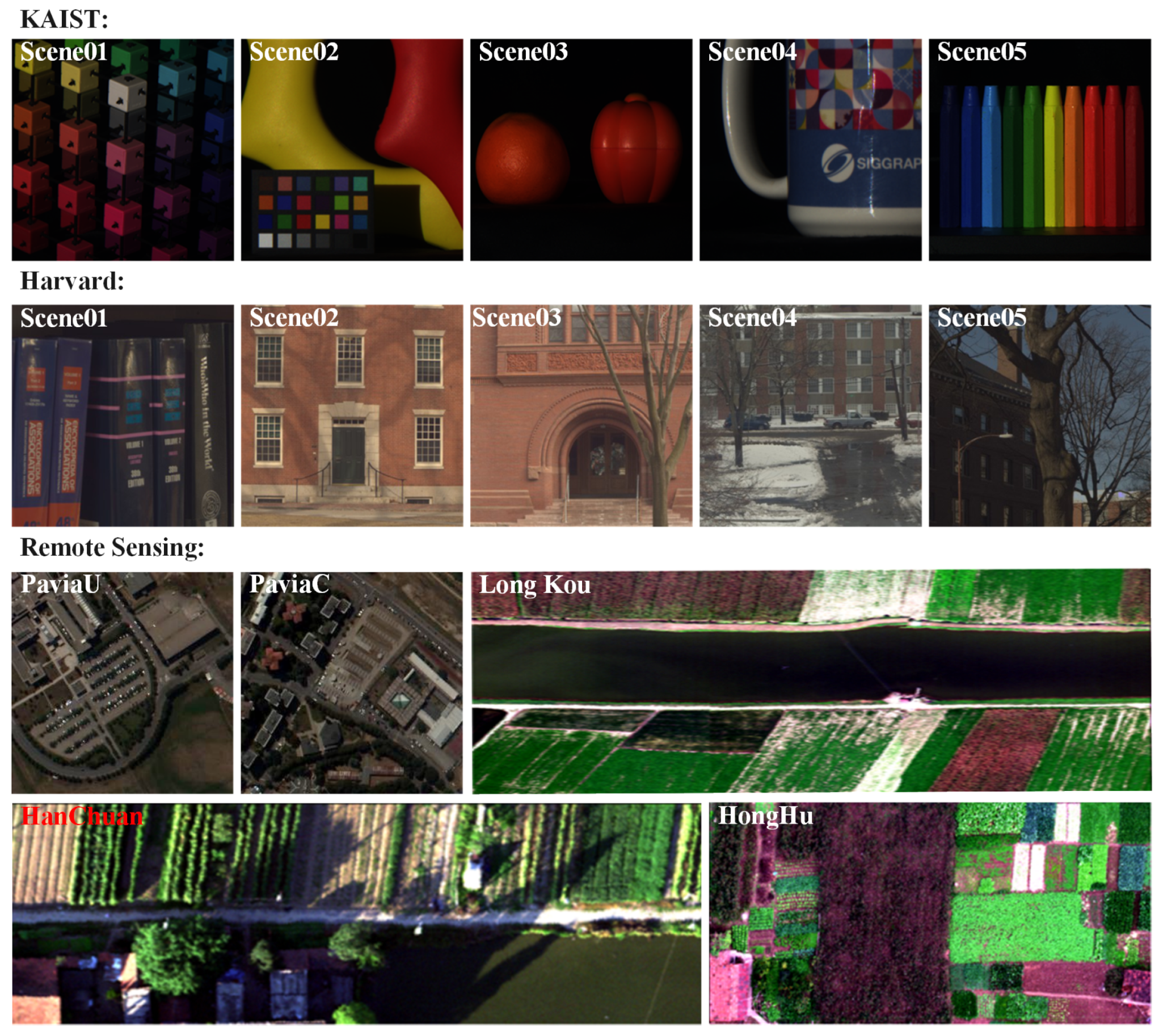
To validate the reconstruction performance of the proposed algorithm, the calibration of the compressed spectral imaging system in reference [33] has been thoroughly studied. Experimental data from the commonly used KAIST [34] and Harvard [35] hyperspectral datasets along with five hyperspectral remote sensing datasets were used for testing. These datasets include Pavia University (PaviaU), Pavia Center (PaviaC), LongKou, HanChuan, and HongHu [36,37]. Specifically, PaviaU and PaviaC contain buildings and roads, LongKou contains remote sensing data including roads, houses, and six types of crops (corn, cotton, sesame, broad-leaf soybean, narrow-leaf soybean, and rice), HanChuan contains various categories of remote sensing data such as buildings, water, and farmland, and HongHu contains remote sensing data from a farmland test area containing crops such as Chinese cabbage, cabbage, and carrots. The five remote sensing datasets were cropped based on mask size, and the specific data specifications are shown in Table 1.

Table 1. Specifications of the datasets used in the experiment.

Testing Scene	Wavelength/nm	Experimental Data	SD-CASSI	RGB
KAIST	450–650	$256\times 256\times 28$	$256\times 310$	$256\times 256\times 3$
Harvard	420–720	$256\times 256\times 31$	$256\times 316$	$256\times 256\times 3$
PaviaU	430–860	$256\times 256\times 34$	$256\times 322$	$256\times 256\times 3$
PaviaC	430–860	$256\times 256\times 34$	$256\times 322$	$256\times 256\times 3$
LongKou	400–700	$256\times 256\times 35$	$256\times 324$	$256\times 256\times 3$
HanChuan	400–700	$256\times 256\times 35$	$256\times 324$	$256\times 256\times 3$
HongHu	400–700	$256\times 256\times 35$	$256\times 324$	$256\times 256\times 3$

In the experimental process, the parameters for the objective function (16), denoted as ${\rho }_2$ and $\eta$, were set to 0.03 and 0.1, respectively. The experimental evaluation metrics included PSNR, SSIM, SAM, correlation coefficient (CC), root mean squared error (RMSE), and relative dimensionless global error in synthesis (ERGAS), which were used to evaluate the reconstruction results. For the KAIST hyperspectral dataset, five common scenes were selected for experimental comparison, with the experimental settings consistent with those inrefs. [17,38]. The Harvard dataset, consisting of 31 channels of real indoor and outdoor hyperspectral data, was used for training, and five common scenes were selected for testing, as shown in Figure 3. To facilitate comparison, the reconstruction experiments were conducted on a computer with the following configuration: Intel Core i9-14900HX CPU 2.2 GHz, 32 GB RAM, Nvidia GeForce RTX 4070 Ti SUPER GPU.

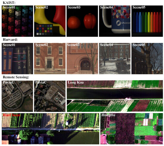
Figure 3. RGB images from the KAIST, Harvard, and hyperspectral remote sensing datasets.

3.2. Analysis of Reconstruction Results

3.2.1. Experiments on KAIST Dataset

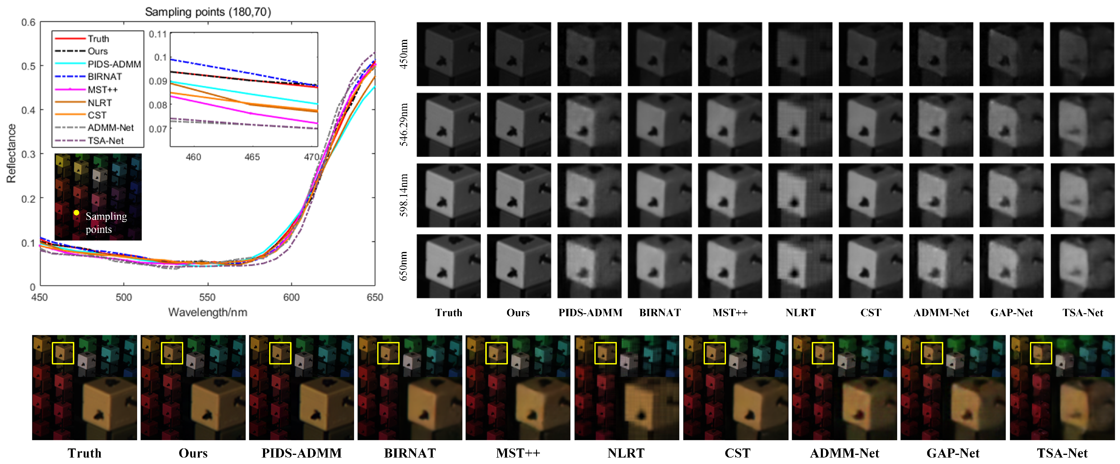
For the KAIST hyperspectral data, the proposed method was compared with algorithms such as BiSRNet [38], ADMM-Net [39], GAP-Net [40], MST++ [41], CST [42], $\lambda$-Net [43], TSA-Net [44], BIRNAT [45], NLRT [46], and PIDS-ADMM [29]. The reconstruction results are shown in Table 2. It can be seen that the quality of the reconstruction results with the method proposed in this paper is significantly improved compared to existing state-of-the-art (SOTA) methods. The PSNR is increased by 2.22 dB, the SSIM is increased by 1.4%, and the SAM is decreased by 0.1%. The evaluation metrics of CC, RMSE, and ERGAS further demonstrate that the proposed method exhibits better generalization across five common scenes, with CC reaching 99.5% and both RMSE and ERGAS showing the best results. Altogether, these results validate the effectiveness of the proposed method.

Table 2. Comparison of reconstruction results with different methods in KAIST scenes.

Testing Scene	Evaluation Method	$\mathit{\lambda }$-Net	BiSRNet	TSA-Net	GAP-Net	ADMM-Net	CST	MST++	BIRNAT	NLRT	PIDS-ADMM	Ours
01	PSNR/dB	27.73	29.17	31.01	31.01	33.56	36.27	40.47	37.69	35.07	40.63	44.96
	SSIM	0.734	0.788	0.857	0.896	0.898	0.947	0.980	0.955	0.955	0.950	0.986
	SAM	0.300	0.271	0.184	0.222	0.223	0.134	0.144	0.145	0.201	0.255	0.143
	CC	0.908	0.935	0.958	0.974	0.977	0.987	0.987	0.991	0.980	0.992	0.998
	RMSE	10.46	8.93	7.14	5.61	5.36	3.83	4.08	3.32	4.85	6.38	3.06
	ERGAS	1.732	1.597	1.435	1.272	1.240	1.066	1.082	0.974	1.170	2.305	0.947
02	PSNR/dB	28.94	28.80	32.20	34.23	35.09	37.09	37.70	40.46	39.57	42.00	43.35
	SSIM	0.831	0.810	0.909	0.925	0.926	0.954	0.968	0.967	0.974	0.969	0.975
	SAM	0.273	0.213	0.136	0.154	0.148	0.095	0.093	0.086	0.046	0.091	0.078
	CC	0.928	0.941	0.969	0.982	0.984	0.989	0.989	0.995	0.989	0.996	0.997
	RMSE	9.18	9.44	6.38	5.1	4.59	3.57	3.57	2.30	3.83	5.36	2.55
	ERGAS	1.512	1.478	1.244	1.071	1.029	0.937	0.946	0.741	0.922	0.913	0.681
03	PSNR/dB	37.77	35.71	39.48	41.00	40.43	41.49	43.88	45.33	46.56	49.61	47.93
	SSIM	0.914	0.902	0.952	0.966	0.964	0.967	0.984	0.983	0.985	0.986	0.987
	SAM	0.229	0.310	0.194	0.217	0.216	0.167	0.183	0.147	0.143	0.160	0.142
	CC	0.867	0.83	0.926	0.947	0.94	0.953	0.964	0.973	0.976	0.988	0.986
	RMSE	3.57	4.59	2.81	2.55	2.55	2.30	1.79	1.53	1.28	2.04	1.28
	ERGAS	3.819	4.255	3.376	3.061	3.239	3.227	2.782	2.585	2.433	2.227	2.148
04	PSNR/dB	26.72	28.13	29.69	31.38	31.91	33.14	37.75	35.48	32.58	40.49	41.47
	SSIM	0.791	0.817	0.879	0.916	0.920	0.949	0.983	0.962	0.916	0.984	0.986
	SAM	0.296	0.205	0.136	0.154	0.153	0.100	0.103	0.089	0.122	0.085	0.086
	CC	0.948	0.963	0.975	0.983	0.986	0.988	0.989	0.993	0.978	0.997	0.998
	RMSE	11.73	9.95	8.42	6.89	6.38	5.61	5.61	4.34	7.40	5.61	4.08
	ERGAS	0.905	0.835	0.763	0.692	0.671	0.628	0.625	0.547	0.731	0.630	0.515
05	PSNR/dB	28.69	29.42	31.52	33.61	33.48	35.21	38.82	39.29	40.67	39.05	43.98
	SSIM	0.789	0.820	0.898	0.912	0.908	0.944	0.980	0.965	0.978	0.958	0.983
	SAM	0.275	0.220	0.151	0.161	0.158	0.123	0.119	0.093	0.099	0.143	0.106
	CC	0.958	0.962	0.978	0.987	0.986	0.99	0.992	0.996	0.992	0.996	0.998
	RMSE	9.44	8.67	6.89	5.36	5.61	4.59	4.08	2.81	3.83	4.59	3.57
	ERGAS	1.403	1.348	1.203	1.054	1.055	0.99	0.926	0.753	0.921	0.964	0.765
Average	PSNR/dB	29.97	30.25	32.78	34.66	34.89	36.64	39.72	39.65	38.89	42.36	44.58
	SSIM	0.912	0.827	0.899	0.923	0.923	0.952	0.979	0.967	0.968	0.969	0.983
	SAM	0.275	0.244	0.160	0.182	0.180	0.124	0.128	0.112	0.122	0.147	0.111
	CC	0.922	0.927	0.962	0.975	0.975	0.982	0.984	0.990	0.983	0.994	0.995
	RMSE	8.93	8.34	6.38	5.10	4.85	4.08	3.83	2.81	4.08	4.85	2.81
	ERGAS	1.874	1.902	1.604	1.430	1.447	1.370	1.272	1.120	1.235	1.408	1.011

Using KAIST Scene 01 from the test set, the reconstruction results of the nine algorithms were visually compared, as shown in Figure 4. Pseudocolor images were generated for the 3rd, 15th, and 25th bands of each method’s prediction results to visually compare the reconstruction outcomes. Additionally, localized magnified comparisons of the reconstruction results for four band images were selected. The comparison reveals that the proposed method achieves high reconstruction quality across different band images, retaining more texture detail information. Among them, the NLRT iterative reconstruction algorithm shows block effect distortions, leading to discontinuous edges in the reconstruction results. The end-to-end reconstruction algorithm can achieve relatively accurate spatial dimension reconstruction, and the fitting degree in the spectral dimension is also improved, although the edges in the reconstruction results appear somewhat blurred. The BIRNAT reconstruction method is closest to the results of our algorithm, with a very small difference in spectral curve fitting between the two; however, the average SAM values for different scenes validate the better spectral curve restoration offered by the proposed method. Visually, the reconstruction results from the proposed method have sharper and clearer edges, retaining more high-frequency detail information. In addition, the surfaces of the solid-color block areas are smoother, further demonstrating the superiority of the proposed method.

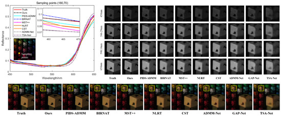
Figure 4. Selected spectral curves of the pixel point with coordinates (180, 70), showing a visual comparison of different methods in the spectral dimension and comparing the pseudocolor images and local spatial detail information under different wavelengths.

3.2.2. Experiments on Harvard Dataset

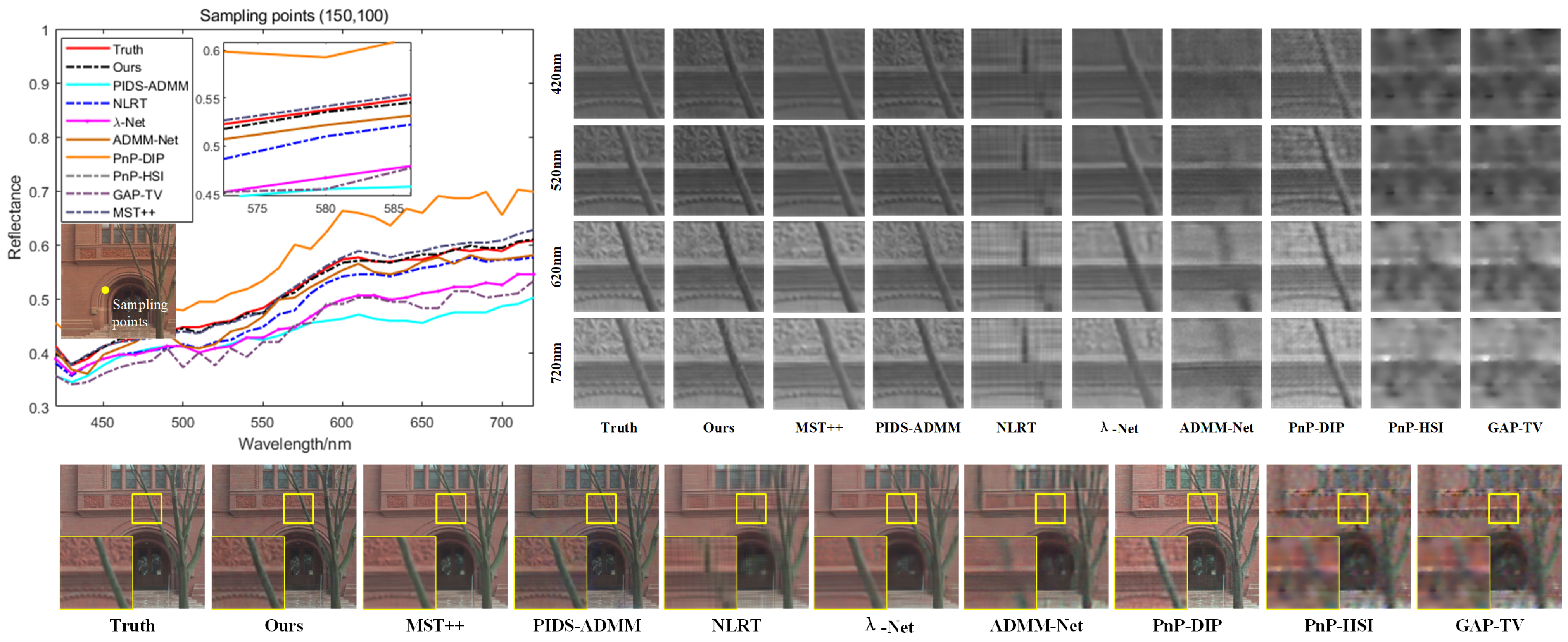
On the Harvard hyperspectral dataset, the proposed method was compared with five iterative reconstruction algorithms: GAP-TV [22], PnP-HSI [47], PnP-DIP [17], NLRT, PIDS-ADMM, as well as five deep reconstruction algorithms: ADMM-Net, BiSRNet, $\lambda$-Net, CST, and MST++. The reconstruction results are shown in Table 3. The comparison reveals that the proposed method significantly improves reconstruction quality, with PSNR increasing by 2.22 dB, SSIM improving by 0.5%, SAM being comparable to SOTA methods, and the CC evaluation metric reaching 99%. Additionally, the proposed method achieves superior results in terms of RMSE and ERGAS, further validating its effectiveness. To clearly compare the detailed information of the reconstruction results, Scene 03 was selected as an example and pseudocolor images of the 5th, 12th, and 25th bands were generated for visual comparison of the detailed information. Additionally, images of four bands were selected for local magnification comparison, as shown in Figure 5.

Table 3. Comparison of reconstruction results from different methods in Harvard scenes.

Testing Scene	Evaluation Method	Gap-TV	PnP-HSI	PnP-DIP	ADMM-Net	BiSRNet	$\mathit{\lambda }$-Net	NLRT	CST	PIDS-ADMM	MST++	Ours
01	PSNR/dB	26.23	27.17	28.13	28.44	28.87	31.69	31.97	34.8	35.39	36.15	37.55
	SSIM	0.648	0.752	0.88	0.781	0.819	0.884	0.892	0.942	0.955	0.957	0.953
	SAM	0.145	0.085	0.061	0.082	0.082	0.051	0.044	0.036	0.054	0.030	0.036
	CC	0.861	0.886	0.978	0.92	0.928	0.959	0.962	0.980	0.982	0.985	0.988
	RMSE	12.46	11.19	10.01	9.72	9.254	6.72	6.49	4.71	7.91	4.04	4.99
	ERGAS	0.651	0.617	0.582	0.576	0.561	0.486	0.478	0.470	0.400	0.517	0.371
02	PSNR/dB	22.53	23.52	31.25	25.29	26.88	28.18	30.55	32.63	36.51	34.68	36.88
	SSIM	0.580	0.581	0.890	0.652	0.754	0.784	0.852	0.867	0.958	0.901	0.962
	SAM	0.072	0.072	0.036	0.051	0.044	0.034	0.027	0.025	0.030	0.023	0.022
	CC	0.757	0.757	0.981	0.876	0.919	0.937	0.964	0.978	0.990	0.987	0.990
	RMSE	19.07	19.08	7.00	13.95	11.62	10.05	7.64	6.00	12.27	4.76	3.97
	ERGAS	0.398	0.398	0.240	0.337	0.310	0.311	0.288	0.250	0.223	0.316	0.199
03	PSNR/dB	25.19	25.27	26.29	27.31	27.61	29.76	29.7	32.46	32.88	34.17	36.31
	SSIM	0.612	0.782	0.803	0.672	0.725	0.790	0.789	0.869	0.941	0.905	0.946
	SAM	0.058	0.048	0.046	0.051	0.049	0.034	0.032	0.026	0.046	0.03	0.026
	CC	0.873	0.874	0.969	0.926	0.928	0.956	0.956	0.976	0.979	0.984	0.989
	RMSE	14.05	14.06	17.77	11.05	10.66	8.32	8.43	6.09	13.14	5.01	4.91
	ERGAS	0.343	0.343	0.382	0.302	0.300	0.315	0.264	0.264	0.226	0.322	0.205
04	PSNR/dB	24.85	26.82	25.51	27.7	28.84	29.37	29.67	32.59	37.07	34.32	40.16
	SSIM	0.623	0.723	0.817	0.711	0.777	0.795	0.793	0.888	0.97	0.921	0.976
	SAM	0.078	0.068	0.048	0.052	0.039	0.037	0.030	0.034	0.031	0.035	0.021
	CC	0.878	0.878	0.975	0.939	0.953	0.958	0.960	0.980	0.993	0.987	0.996
	RMSE	14.61	14.61	21.49	10.52	9.28	8.72	8.47	6.02	9.17	4.93	4.55
	ERGAS	0.468	0.468	0.566	0.397	0.371	0.367	0.360	0.354	0.299	0.370	0.271
05	PSNR/dB	28.52	28.71	26.9	30.17	30.97	32.18	30.84	35.73	34.96	35.48	37.01
	SSIM	0.704	0.764	0.844	0.758	0.800	0.834	0.783	0.916	0.937	0.942	0.946
	SAM	0.094	0.084	0.074	0.084	0.083	0.062	0.062	0.042	0.075	0.041	0.053
	CC	0.834	0.835	0.96	0.889	0.918	0.932	0.908	0.972	0.973	0.981	0.986
	RMSE	9.65	9.65	11.62	7.96	7.30	6.33	7.46	4.23	5.58	4.45	3.51
	ERGAS	0.840	0.840	0.923	0.764	0.729	0.623	0.681	0.734	0.554	0.650	0.501
Average	PSNR/dB	25.46	26.3	27.62	27.78	28.63	30.24	30.55	33.64	35.36	34.96	37.58
	SSIM	0.633	0.72	0.847	0.715	0.775	0.817	0.822	0.896	0.952	0.926	0.957
	SAM	0.089	0.0714	0.053	0.064	0.059	0.044	0.039	0.033	0.047	0.032	0.032
	CC	0.841	0.846	0.973	0.91	0.929	0.948	0.95	0.977	0.983	0.985	0.99
	RMSE	13.97	13.72	13.58	10.64	9.625	8.03	7.70	5.41	9.61	4.64	4.39
	ERGAS	0.539	0.533	0.539	0.475	0.454	0.420	0.414	0.415	0.341	0.435	0.309

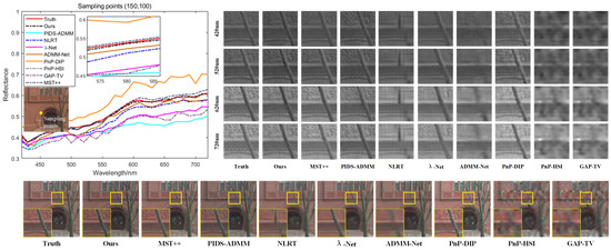
Figure 5. Selected spectral curves of the pixel point with coordinates (150, 100), showing a visual comparison of different methods in the spectral dimension and comparing the pseudocolor images and local spatial detail information of different wavelengths.

This comparison shows that the proposed method achieves clearer texture reconstruction results for images of different bands with better balance between high-frequency and low-frequency areas, resulting in superior reconstruction quality. In terms of spectral consistency, the spectral reconstruction results of the proposed method are closest to the true spectral data, allowing for more accurate recovery of the subtle differences between the original spectral signal channels. This further validates the advantages of the proposed method in long-range spectral correlation.

3.2.3. Experiments on Remote Sensing Datasets

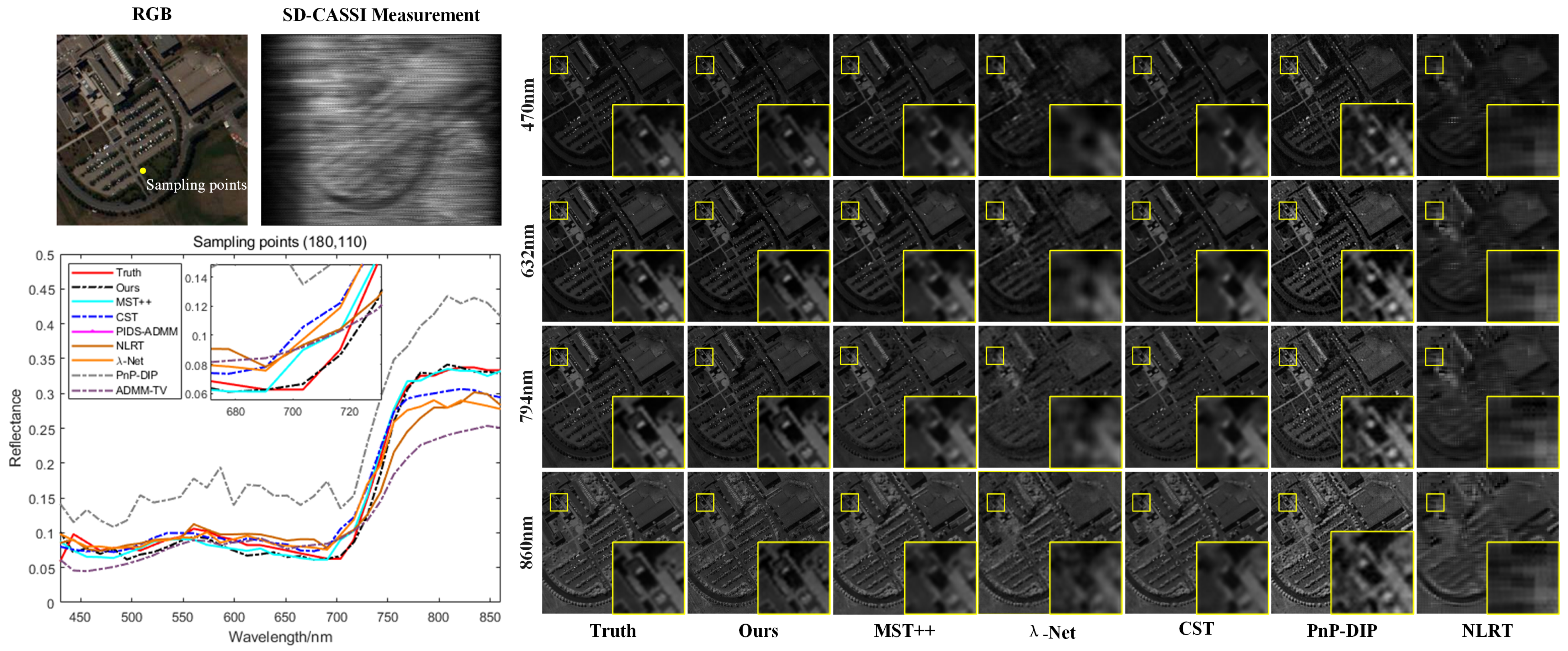
We conducted experimental validation using five remote sensing datasets: PaviaU, PaviaC, LongKou, HanChuan, and HongHu. The PaviaU and PaviaC datasets were collected by the ROSIS sensor over the University of Pavia and the Pavia Center, with spatial resolutions of $610\times 610$ and $1096\times 1096$, respectively. After removing noisy bands, the effective band numbers were 103 and 102. We selected the first 102 bands of PaviaU to match the bands of PaviaC, then selected one image every three bands. The data were cropped to match the mask size. The LongKou, HanChuan, and HongHu datasets were captured by the Headwall Nano-Hyperspec imaging sensor using 400–700 nm wavelength bands with intervals ranging from 6.67 nm to 8.89 nm. To evaluate the reconstruction performance of the proposed method on hyperspectral remote sensing data, we compared it with four iterative methods: ADMM-TV [48], PnP-DIP, NLRT, PIDS-ADMM, as well as three deep reconstruction methods: $\lambda$-Net, CST, and MST++. The reconstruction results are shown in Table 4.

Table 4. Comparison of reconstruction results on hyperspectral remote sensing data.

Testing Scene	Evaluation Method	ADMM-TV	PnP-DIP	$\mathit{\lambda }$-Net	NLRT	PIDS-ADMM	CST	MST++	Ours
PaviaU	PSNR/dB	26.54	25.72	27.83	26.74	24.49	30.03	30.97	32.28
	SSIM	0.638	0.776	0.721	0.647	0.667	0.825	0.859	0.895
	SAM	0.179	0.152	0.165	0.166	0.301	0.118	0.111	0.116
	CC	0.705	0.922	0.825	0.750	0.707	0.900	0.920	0.939
	RMSE	13.82	13.59	10.4	12.24	13.79	8.06	7.24	6.99
	ERGAS	1.197	1.155	1.072	1.144	1.196	0.938	0.888	0.773
PaviaC	PSNR/dB	25.52	27.82	27.08	25.61	24.46	29.8	30.38	31.68
	SSIM	0.57	0.803	0.669	0.66	0.657	0.806	0.834	0.887
	SAM	0.221	0.204	0.214	0.188	0.331	0.146	0.139	0.129
	CC	0.796	0.953	0.884	0.829	0.789	0.940	0.948	0.954
	RMSE	15.59	10.49	11.31	13.66	16	8.27	7.74	6.49
	ERGAS	1.222	1.002	1.073	1.156	1.200	0.909	0.880	0.786
LongKou	PSNR/dB	26.85	23.89	25.16	30.37	24.2	26.32	27.53	29.45
	SSIM	0.758	0.675	0.692	0.791	0.681	0.703	0.711	0.81
	SAM	0.082	0.153	0.129	0.056	0.153	0.119	0.118	0.081
	CC	0.815	0.797	0.901	0.912	0.912	0.918	0.92	0.934
	RMSE	11.93	16.33	43.20	8.14	16.18	23.23	22.87	10.50
	ERGAS	1.492	1.563	1.192	0.811	1.825	0.992	0.851	0.820
HanChuan	PSNR/dB	24.31	26.50	24.93	26.23	23.63	26.32	26.53	27.13
	SSIM	0.665	0.744	0.763	0.732	0.706	0.803	0.811	0.834
	SAM	0.118	0.125	0.122	0.116	0.255	0.119	0.118	0.098
	CC	0.91	0.933	0.904	0.930	0.913	0.918	0.920	0.947
	RMSE	15.91	12.27	33.47	12.83	16.83	23.23	22.87	11.49
	ERGAS	1.879	1.365	1.704	1.498	1.866	1.028	1.044	0.935
HongHu	PSNR/dB	32.79	22.29	27.45	34.40	30.00	28.91	29.77	30.39
	SSIM	0.785	0.663	0.807	0.816	0.663	0.819	0.829	0.892
	SAM	0.1	0.103	0.133	0.092	0.139	0.128	0.127	0.086
	CC	0.1	0.103	0.133	0.092	0.139	0.128	0.127	0.086
	RMSE	5.99	21.28	11.25	5.04	8.159	7.25	6.71	4.58
	ERGAS	0.887	1.157	0.916	0.893	0.986	0.959	0.909	0.824
Average	PSNR/dB	26.75	25.25	26.49	28.59	25.36	28.28	29.04	30.19
	SSIM	0.66	0.733	0.73	0.704	0.675	0.791	0.809	0.867
	SAM	0.14	0.148	0.153	0.130	0.236	0.126	0.123	0.102
	CC	0.820	0.901	0.862	0.866	0.822	0.897	0.919	0.935
	RMSE	12.65	14.8	21.93	10.38	14.19	14.00	14.19	8.01
	ERGAS	1.335	1.248	1.191	1.100	1.415	0.965	0.914	0.828

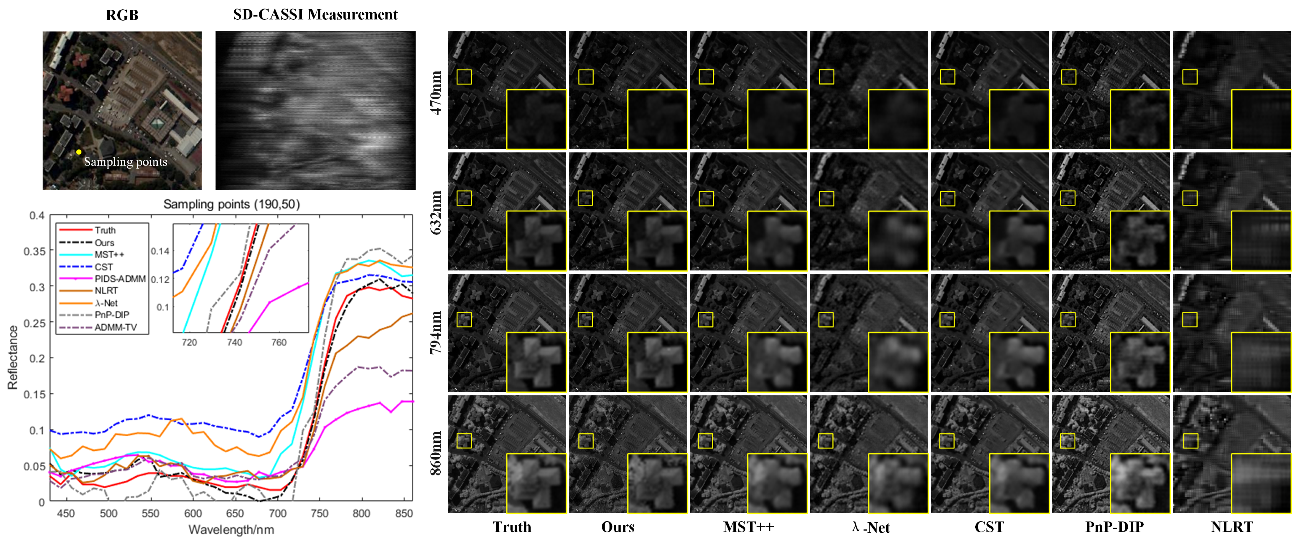
The comparison results show that the method proposed in this paper achieves better reconstruction performance, with higher average PSNR and SSIM, and improved spectral consistency. Compared to the MST++ reconstruction method, PSNR is increased by 1.15 dB, SSIM is improved by 5.8%, SAM is reduced by 2.1%, and CC is increased by 1.6%. The RMSE results show little difference, and the ERGA of the proposed method is the lowest, further demonstrating its superior generalization across different remote sensing datasets. Figure 6 and Figure 7 illustrate the reconstruction results for the PaviaU and PaviaC datasets. By comparing the spatial detail information at different wavelengths, it is evident that the proposed method performs better in reconstructing both high-frequency edge information and low-frequency details, resulting in clearer outcomes. Comparing the spectral curves of the different reconstruction results indicates that the proposed method is able to closely match the amplitude variations of the true spectral curves, achieving better spectral fidelity and further confirming its effectiveness.

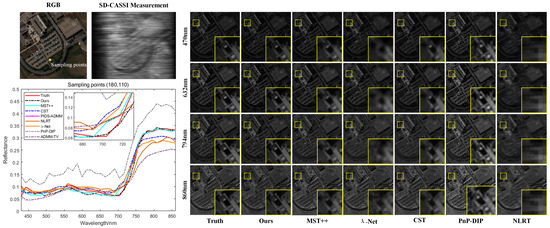
Figure 6. Comparison of the spectral consistency of reconstruction results with different methods on the PaviaU hyperspectral remote sensing datast at sample point coordinates (180, 110), along with a comparison of the spatial detail information of the reconstruction results at different wavelengths.

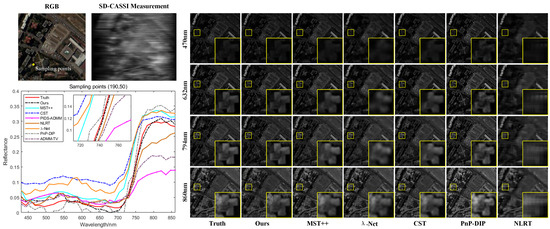
Figure 7. Comparison of the spectral consistency of reconstruction results with different methods on the PaviaC hyperspectral remote sensing dataset at sample point coordinates (190, 50), along with a comparison of the spatial detail information of the reconstruction results at different wavelengths.

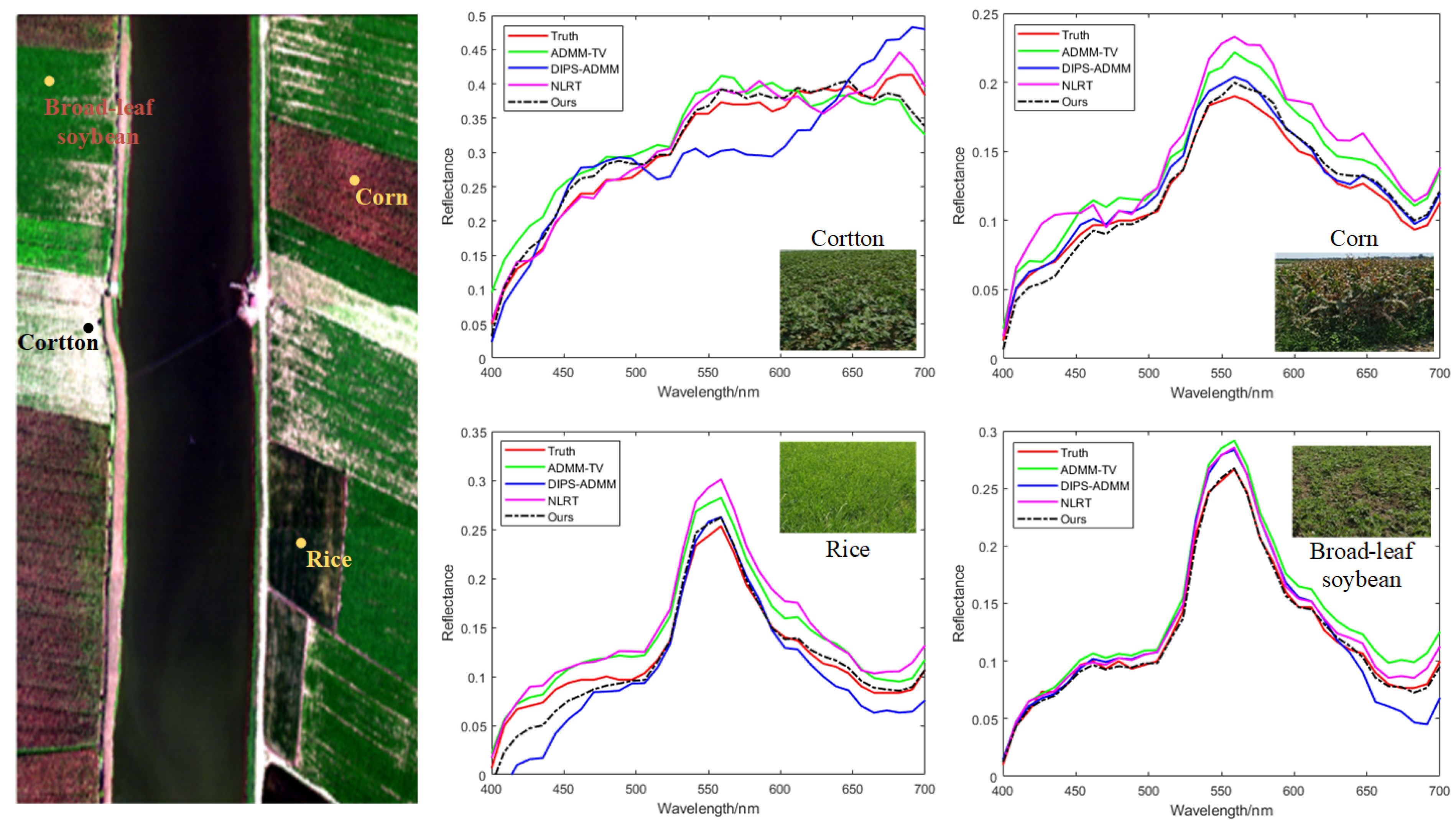
Figure 8 shows a comparison of the reconstruction results of the spectral information for different crop types in the LongKou remote sensing dataset. The reconstruction results for cotton, corn, rice, and broad-leaf soybean were selected for comparison. It can be observed that the proposed method maintains better consistency with the true spectra across different crop types, further validating the effectiveness of our approach.

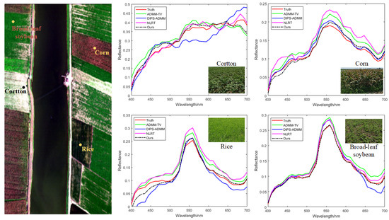
Figure 8. Comparison of spectral reconstruction results for different crops.

4. Discussion

4.1. Ablation Study on the Hyperparameters of the Prior Model

The quality of the prior model’s predictions is a major factor affecting the reconstruction quality. The higher the prediction quality of the prior model, the better the constraint performance of the total variation regularization during the reconstruction process. In the method proposed in this paper, the parameter that influences the prediction quality of the model is primarily determined by the number of regression trees.

To further investigate the impact of the number of regression trees on the predictions of the prior model, we conducted a comparative study using PaviaU and PaviaC remote sensing data at different numbers of regression trees, as shown in Table 5. The comparative results indicate that the prediction quality of the prior model and the reconstruction quality gradually increase with the increasing number of regression trees. Both PaviaU and PaviaC demonstrate the same trend in prediction and reconstruction quality as the number of regression trees increases. When the number of regression trees reaches 90, the proposed method achieves optimal prediction and reconstruction efficiency, yielding superior reconstruction results in a shorter time.

Table 5. Comparison of predictive results from prior models and hyperspectral reconstruction results under different regression tree configurations.

Model	Testing Scene	Evaluation Method	20	30	40	50	60	80	90	100
GBM	PaviaU	PSNR/dB SSIM Time/s	29.32 0.827 0.206	29.75 0.842 0.286	29.98 0.850 0.303	30.08 0.855 0.357	30.18 0.859 0.404	30.35 0.864 0.503	30.38 0.865 0.550	30.40 0.865 0.603
	PaviaC	PSNR/dB SSIM Time/s	28.22 0.819 0.183	28.50 0.834 0.243	28.77 0.844 0.311	28.86 0.850 0.341	28.96 0.854 0.392	29.17 0.861 0.489	29.21 0.862 0.523	29.21 0.862 0.583
SD-CASSI	PaviaU	PSNR/dB SSIM Time/s	31.69 0.887 134.0	31.70 0.887 133.5	31.70 0.887 136.2	31.74 0.888 133.7	31.77 0.885 135.1	31.87 0.890 134.6	32.15 0.895 133.7	32.16 0.895 135.7
	PaviaC	PSNR/dB SSIM Time/s	30.99 0.868 139.4	31.34 0.880 138.1	31.33 0.880 141.6	31.34 0.880 143.2	31.38 0.881 140.6	31.49 0.883 145.8	31.68 0.887 133.2	31.68 0.887 141.3

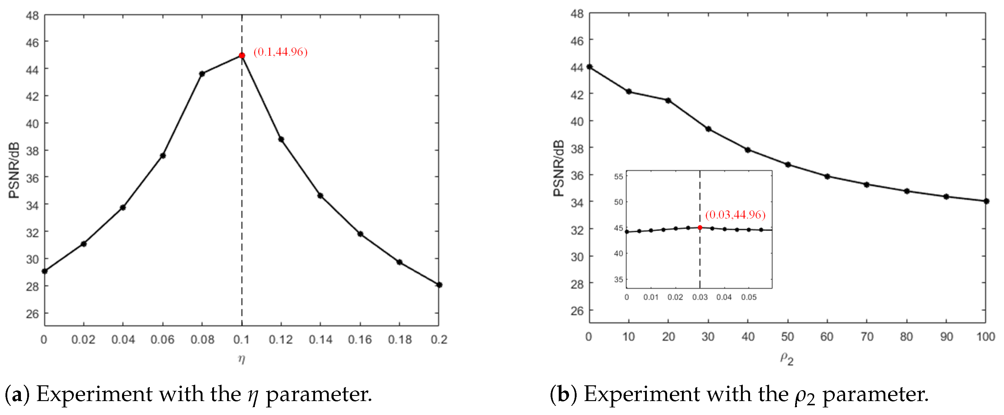
Figure 9 demonstrates the impact of the hyperparameter settings in the objective function (16) on the experiment. The tests were conducted by varying the value of each parameter while keeping the others fixed, using KAIST Scene01 as an example. Specifically, Figure 9a shows how the PSNR changes with the variation of the $\eta$ parameter, while Figure 9b shows the PSNR variation with the change in ${\rho }_2$. From this comparison, it can be observed that the highest reconstruction quality is achieved when $\eta$ is set to 0.1. The PSNR first increases and then decreases as ${\rho }_2$ changes, and the algorithm model achieves the best reconstruction quality when ${\rho }_2$ is set to 0.03.

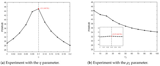
Figure 9. Impact of hyperparameter settings on reconstruction quality.

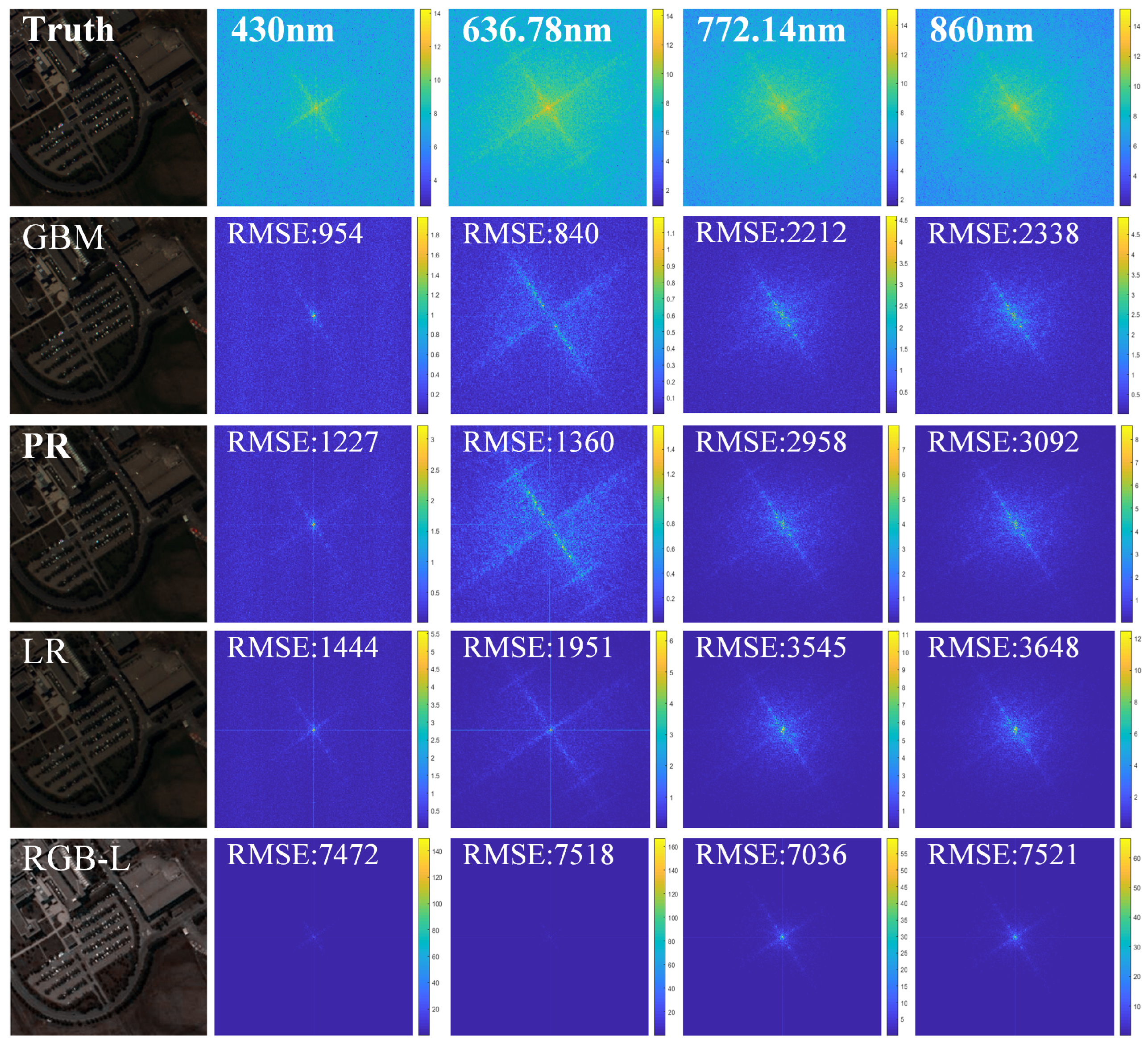
4.2. Analysis of Prior Model Predictive Performance

The distribution of high-frequency and low-frequency data in hyperspectral images varies at different wavelengths. To validate the prediction performance of the proposed method across different frequency distributions at various wavelengths, we used Scene 04 from the Harvard dataset and the PaviaU hyperspectral remote sensing dataset as examples. The proposed method was compared with several other methods, including Convolutional Neural Network (CNN), Linear Regression (LR), Polynomial Regression (PR), RGB Linear Interpolation (RGB-L), and Nearest Neighbor Interpolation (RGB-N). The evaluation metrics included the PSNR, SSIM, and root mean square error (RMSE) of the spectral distribution after Fourier transformation, which were to assess the prediction results at different wavelengths. The results are shown in Table 6.

Table 6. Comparison of prediction results of different prior models.

Method	Evaluation Method	Harvard Scene 04				PaviaU				Average
		420 nm	520 nm	620 nm	720 nm	430 nm	636.78 nm	772.14 nm	860 nm
LR	PSNR/dB SSIM RMSE	28.10 0.941 2315	30.67 0.979 1716	32.06 0.973 1414	28.94 0.944 2073	30.50 0.686 1444	28.56 0.867 1951	22.37 0.423 3545	22.07 0.401 3648	27.91 0.777 2263
PR	PSNR/dB SSIM RMSE	36.92 0.966 686	37.60 0.980 661	38.41 0.976 587	33.97 0.943 920	31.47 0.698 1227	30.64 0.888 1360	23.75 0.545 2958	23.32 0.510 3092	32.01 0.813 1436
RGB-L	PSNR/dB SSIM RMSE	28.54 0.945 2082	38.08 0.987 737	23.85 0.960 4011	18.70 0.873 7251	17.90 0.449 7472	18.36 0.666 7518	16.62 0.360 7036	15.94 0.298 7521	22.25 0.692 5454
RGB-N	PSNR/dB SSIM RMSE	28.54 0.945 2082	38.16 0.980 574	24.24 0.950 3734	18.70 0.873 7251	17.90 0.449 7472	18.23 0.661 7639	16.47 0.354 7172	15.94 0.298 7521	22.27 0.689 5431
CNN	PSNR/dB SSIM RMSE	25.53 0.850 2960	35.22 0.971 829	22.73 0.887 552	21.93 0.918 817	24.25 0.468 3727	20.47 0.768 5850	16.88 0.369 6838	16.16 0.336 8640	22.90 0.696 3777
GBM	PSNR/dB SSIM RMSE	37.99 0.964 608	38.39 0.977 596	38.96 0.974 552	35.10 0.940 817	33.65 0.791 954	34.83 0.932 840	26.29 0.706 2212	25.78 0.678 2338	33.87 0.870 1115

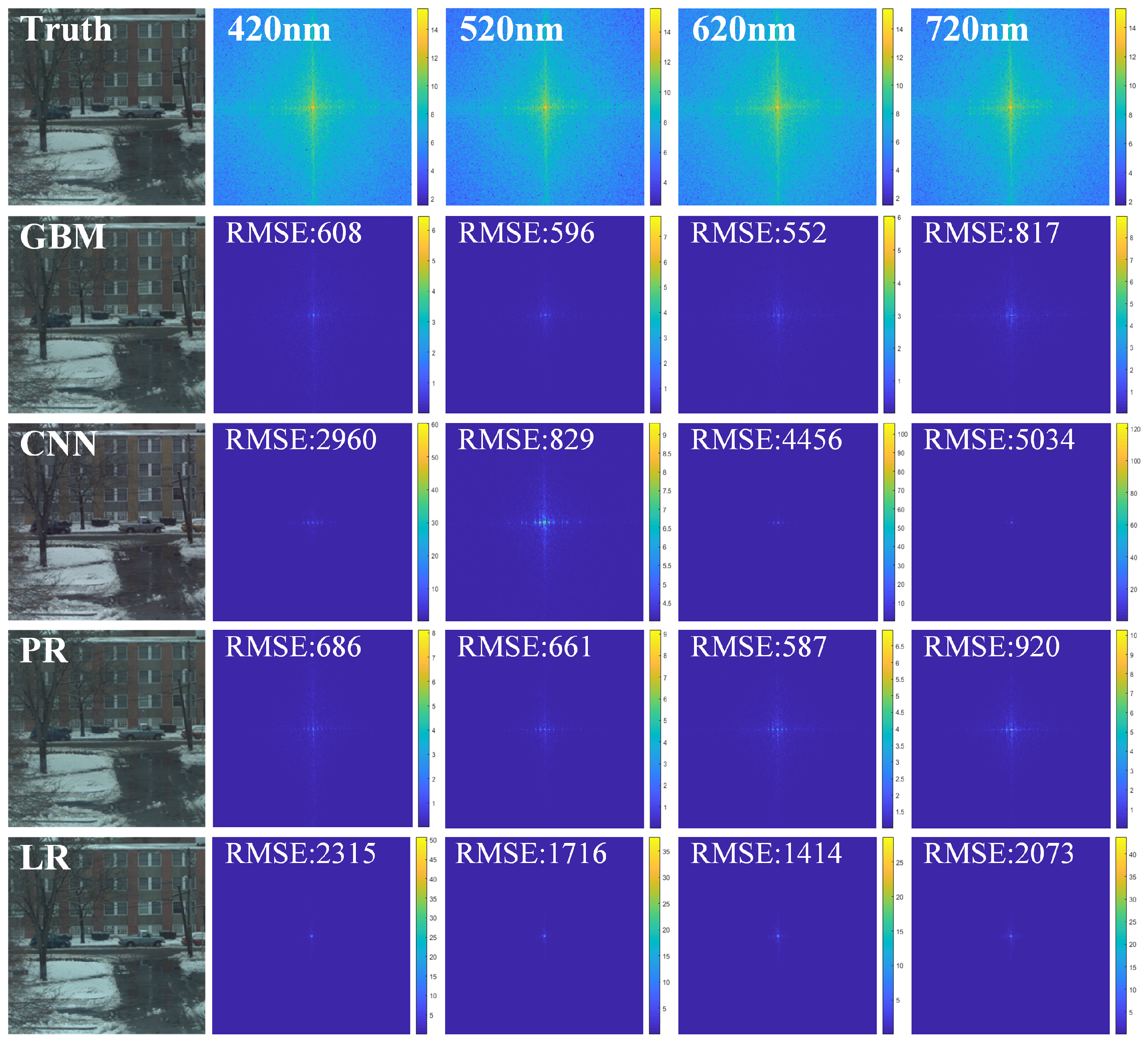
Comparative analysis shows that the proposed method demonstrates better predictive performance for images with different wavelengths and exhibits good generalization ability for hyperspectral data from various scenes. On the Harvard and PaviaU hyperspectral remote sensing datasets, the PSNR increased by 1.86 dB, the SSIM improved by 5.7%, and the RMSE decreased by 321. Pseudocolor images were generated for the 3rd, 13th, and 26th bands of the PaviaU hyperspectral remote sensing dataset, and visual comparisons were made for both the spatial and spectral dimensions, as shown in Figure 10 and Figure 11. To intuitively reflect the prediction performance of the prior models regarding different frequency information, we computed the spectral differences between the predicted results and the prior spectral images using Fourier transformation, presenting these differences in the form of heat maps.

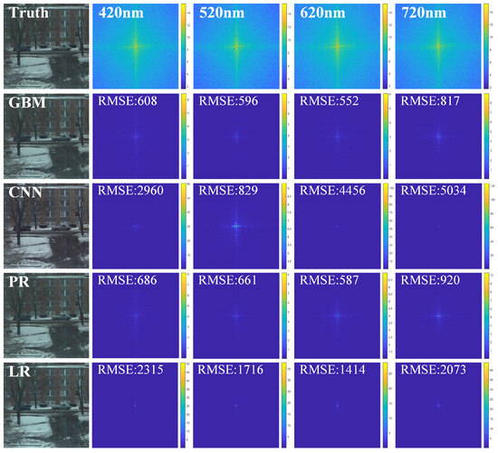
Figure 10. Comparison of pseudocolor images generated from the predictions of different prior models for the Harvard Scene 04 hyperspectral data at the 5th, 12th, and 25th bands, along with the spectral differences of the predictions at different wavelengths.

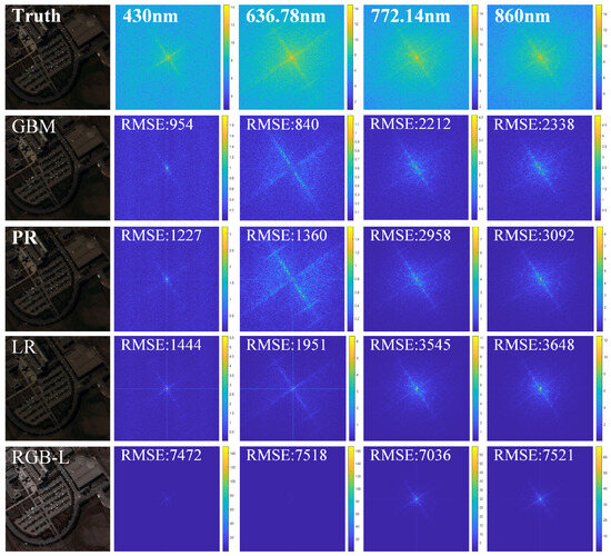
Figure 11. Comparison of pseudocolor images generated from the predictions of different prior models for the PaviaU hyperspectral remote sensing data at the 3rd, 13th, and 26th bands, along with the spectral differences of the predictions at different wavelengths.

By comparing the pseudocolor images, it is evident that the pseudocolor images from the proposed method closely resemble the actual pseudocolor images, demonstrating good spatial structural fidelity and maintaining strong long-range correlation in the spectral dimension. The frequency differences in the predictions at different wavelengths indicate that CNN exhibits good smoothness for low frequencies, but suffers significant information loss in the high-frequency components, while the RGB image interpolation methods exhibit severe information distortion in the spatial and spectral dimensions for wavelengths beyond the visible light range. On the other hand, the proposed method retains more high-frequency detail information, although the results lack a certain degree of smoothness because the predictions were made on a pixelwise basis. This necessitates local smoothing of the predicted results using SDM, thereby establishing more precise regularization constraints for the reconstruction process.

4.3. Ablation Study on the Removal of Algorithm Modules

The effectiveness of the proposed algorithm stems from its joint training of global feature extraction and gradient boosting sampling strategy, local smoothing optimization of the prediction results through SDM, and prior semantic regularization term (PSR). The combination of global feature extraction with a gradient-boosting sampling strategy accelerates model training while enhancing the training weight for high-gradient samples, thereby improving the training efficiency of high-frequency information. The SDM establishes a smoothing constraint based on the coefficient matrix utilizing the local low-rank smooth characteristics of the predicted results, which effectively improves the reconstruction quality of the predictions. To clarify the contributions of each part to the overall reconstruction algorithm, an ablation study was conducted to test the gains of each component using PSNR, SSIM, SAM, and the time required for each part’s operation as the evaluation metrics. The benchmark model employed a traditional regression tree algorithm for feature mapping between RGB images and prior spectral data, allowing us to test the contribution by progressively adding different algorithm modules. Taking KAIST as an example, the average reconstruction results for the five scenes of SD-CASSI are shown in Table 7. Through comparison, it is evident that adding the HA-GBM module to the prior model not only improves the quality of the reconstruction results but also accelerates the model’s prediction speed. PSNR increases by 4.13 dB and SSIM by 0.7%, while SAM decreases by 10.1% and the prediction time is reduced by 6.06 s. Further enhancing the prior model’s prediction quality by adding the SDM module on top of the HA-GBM model results in an additional increase in PSNR by 2.33 dB and SSIM by 0.4%, along with a reduction in SAM of 0.8%. These results confirm that enhancing the local low-rank smoothness of the coefficient matrix is beneficial for improving the quality of the prediction results. The PSR module establishes a regularization term utilizing the semantic similarity between the denoised results and the prior spectral data, thereby transforming the SD-CASSI reconstruction problem into a total variation difference minimization problem. After incorporating the PSR regularization model, the PSNR of SD-CASSI reconstruction for different scenes increases by 2.97 dB, the SSIM improves by 0.8%, and the SAM decreases by 0.3%, further validating the effectiveness of the proposed method.

Table 7. Comparison of the results of the ablation experiments for algorithm module removal.

Baseline Model	HA-GBM	SDM	PSR	PSNR/dB	SSIM	SAM	Time/s
√				35.15	0.964	0.223	7
√	√			39.28	0.971	0.122	0.94
√	√	√		41.61	0.975	0.114	2.95
√	√	√	√	44.58	0.983	0.111	5.6

The symbol “√” indicates whether the corresponding module is selected in the experimental configuration displayed for the respective row.

4.4. Comparison of Computational Complexity and Reconstruction Time

Table 8 compares the computational parameters and reconstruction times of the proposed method and SOTA methods in the KAIST scene reconstruction process. In terms of spatial complexity, the proposed method has a parameter count of 1.76 M, which is relatively small, indicating that the model structure is compact and the spatial resources required for operation are limited. This allows the method to achieve better reconstruction quality under a relatively small parameter count. In terms of time complexity, the reconstruction time for the proposed method is 9.49 s. The reconstruction time is somewhat increased due to the iterative calculations required during the solving process.

Table 8. Comparison of computational complexity and actual reconstruction times for different reconstruction methods.

Method	PSNR (dB)/SSIM	Params/M	Processor Type	Time/s
ADMM-TV	24.36/0.669	-	CPU	459
$\lambda$-Net	28.53/0.841	62.64	CPU	1.6
ADMM-Net	33.12/0.918	4.27	GPU	0.57
CST	36.12/0.957	2.37	GPU	0.73
MST++	35.99/0.951	1.33	GPU	0.73
BIRNAT	37.58/0.960	4.27	GPU	2.12
NLRT	38.89/0.968	-	GPU	2764
PIDS-ADMM	40.36/0.969	-	GPU	74.9
Ours	44.58/0.983	1.76	GPU	9.49

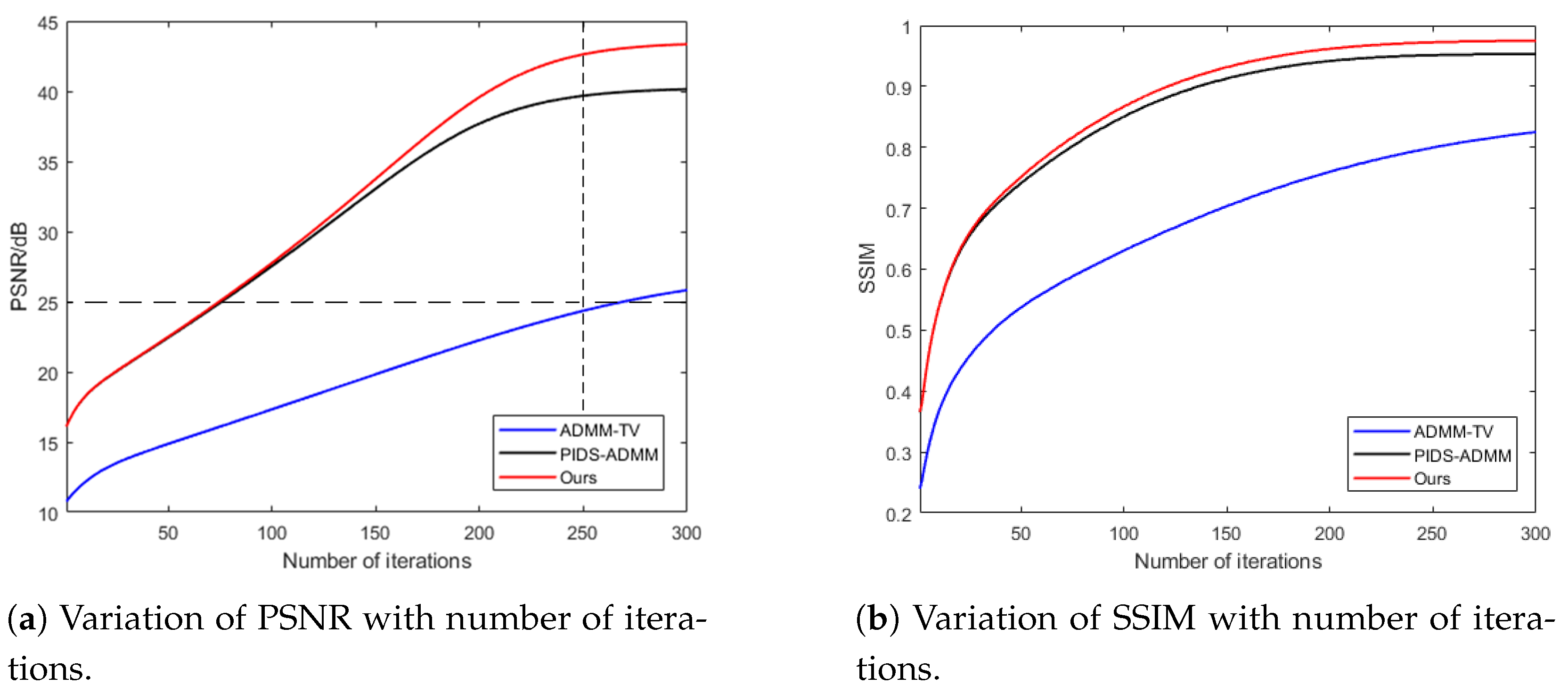
Figure 12 shows the variation in reconstruction quality with increasing iterations for ADMM-TV, PIDS-ADMM, and the proposed method. All three comparison methods use the ADMM optimization algorithm as the solving framework. ADMM-TV is a regularized reconstruction method that adds a total variation smoothing constraint to the reconstruction result, while PIDS-ADMM is a regularized solving algorithm based on total the variation while using RGB interpolation to establish constraints for the reconstruction result. The comparison shows that the proposed method achieves higher reconstruction quality with the same number of iterations and requires fewer iterations for the same reconstruction quality. The proposed method establishes a regularization term for the reconstruction process by considering the difference between the reconstruction result and the denoised result, which effectively strengthens the constraints in the solution space. By introducing more prior information, the proposed algorithm can more accurately locate the approximate range of the optimal solution and accelerate convergence. Therefore, establishing a more accurate regularization term helps to further improve reconstruction quality, reduce time consumption, and enhance computational efficiency by improving computer configurations and enabling parallel processing. Compared to the ADMM-TV algorithm, the proposed method not only improves reconstruction quality by establishing more precise constraints but also helps the algorithm escape local optima and accelerates convergence.

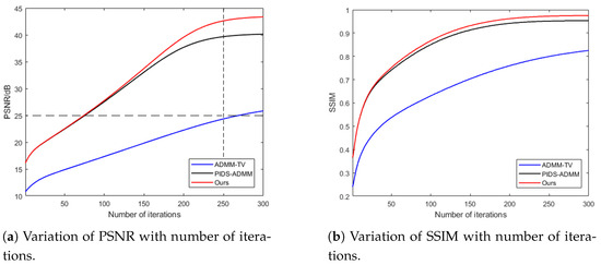
Figure 12. Variation in reconstruction quality with increasing iteration count under the same solving framework for different regularization constraint methods.

5. Conclusions

This paper proposes a compressed spectral reconstruction method based on global gradient information and local low-rank priors. Continuous numerical features are discretized into a finite number of intervals, and a gradient boosting sampling strategy is used to enhance the training weights of high-gradient samples. This effectively improves the prior model’s sensitivity to different frequency information, resulting in good prediction quality for hyperspectral data across various scenarios. On both the Harvard dataset and hyperspectral remote sensing datasets, the PSNR increased by at least 1.86 dB, the SSIM improved by at least 5.7%, and the RMSE decreased by 321, leading to better preservation of high-frequency detail information. Additionally, it was validated that enhancing the local smoothness properties of the representative coefficient matrix benefits the prior model by maintaining global structural information while improving local smoothness in the neighborhood. By establishing a regularization term in the reconstruction process based on the semantic similarity between denoised results and prior spectral data, the constraint performance of the regularization term on the solution space can be further improved. The higher the prediction quality of the prior model, the better the constraints of the total variation regularization during the reconstruction process. The reconstruction results from different scenarios indicate that the proposed method demonstrates better sensitivity to different frequency information compared to SOTA methods, effectively preserving image detail and achieving superior spectral reconstruction quality.

References

- Yang, J.; Du, B.; Wang, D.; Zhang, L. ITER: Image-to-Pixel Representation for Weakly Supervised HSI Classification. IEEE Trans. Image Process. 2024, 33, 257–272. [Google Scholar] [CrossRef] [PubMed]
- Pan, B.; Shi, X. Fusing Ascending and Descending Time-Series SAR Images with Dual-Polarized Pixel Attention UNet for Landslide Recognition. Remote Sens. 2023, 15, 5619. [Google Scholar] [CrossRef]
- Meng, Y.; Yuan, Z.; Yang, J.; Liu, P.; Yan, J.; Zhu, H.; Ma, Z.; Jiang, Z.; Zhang, Z.; Mi, X.; et al. Cross-Domain Land Cover Classification of Remote Sensing Images Based on Full-Level Domain Adaptation. IEEE J. Sel. Top. Appl. Earth Obs. Remote Sens. 2024, 17, 11434–11450. [Google Scholar] [CrossRef]
- Ralls, C.; Polyakov, A.Y.; Shandas, V. Scale-Dependent Effects of Urban Canopy Cover, Canopy Volume, and Impervious Surfaces on Near-Surface Air Temperature in a Mid-Sized City. Remote Sens. 2024, 13, 1741. [Google Scholar] [CrossRef]
- Zhang, Q.; Wang, L.; Wang, H.; Chen, Y.; Tian, C.; Shao, Y.; Liu, T. An Improved Framework of Major Function-Oriented Zoning Based on Carrying Capacity: A Case Study of the Yangtze River Delta Region. Remote Sens. 2024, 13, 1732. [Google Scholar] [CrossRef]
- Huang, L.; Luo, R.; Liu, X.; Hao, X. Spectral imaging with deep learning. Light Sci. Appl. 2023, 6, 2047–7538. [Google Scholar] [CrossRef]
- Liu, Y.; Yuan, X.; Suo, J.; Brady, D.J.; Dai, Q. Rank Minimization for Snapshot Compressive Imaging. IEEE Trans. Pattern Anal. Mach. Intell. 2019, 12, 2990–3006. [Google Scholar] [CrossRef]
- Song, L.; Wang, L.; Kim, M.H.; Huang, H. High-Accuracy Image Formation Model for Coded Aperture Snapshot Spectral Imaging. IEEE Trans. Comput. Imaging 2022, 8, 188–200. [Google Scholar] [CrossRef]
- Chen, Y.; Zhang, H.; Wang, Y.; Ying, A.; Zhao, B. ADMM-DSP: A Deep Spectral Image Prior for Snapshot Spectral Image Demosaicing. IEEE Trans. Ind. Inform. 2024, 20, 4795–4805. [Google Scholar] [CrossRef]
- Li, C.; Zhang, B.; Hong, D.; Zhou, J.; Vivone, G.; Li, S.; Chanussot, J. CasFormer: Cascaded transformers for fusion-aware computational hyperspectral imaging. Inf. Fusion 2024, 108, 1566–2535. [Google Scholar] [CrossRef]
- Gelvez, T.; Arguello, H. Nonlocal Low-Rank Abundance Prior for Compressive Spectral Image Fusion. IEEE Trans. Geosci. Remote Sens. 2021, 59, 415–425. [Google Scholar] [CrossRef]
- Gelvez, T.; Bacca, J.; Arguello, H. Interpretable Deep Image Prior Method Inspired In Linear Mixture Model For Compressed Spectral Image Recovery. In Proceedings of the 2021 IEEE International Conference on Image Processing (ICIP), Anchorage, AK, USA, 19–22 September 2021; pp. 1934–1938. [Google Scholar]
- Jacome, R.; Bacca, J.; Arguello, H. Deep-Fusion: An End-To-End Approach for Compressive Spectral Image Fusion. In Proceedings of the 2021 IEEE International Conference on Image Processing (ICIP), Anchorage, AK, USA, 19–22 September 2021; pp. 2903–2907. [Google Scholar]
- Wang, L.; Wu, Z.; Zhong, Y.; Yuan, X. Snapshot spectral compressive imaging reconstruction using convolution and contextual Transformer. Photon. Res. 2022, 10, 1848. [Google Scholar] [CrossRef]
- Donoho, D.L. Compressed sensing. IEEE Trans. Inf. Theory. 2006, 52, 1289–1306. [Google Scholar] [CrossRef]
- Zhu, J.; Zhao, B. Optimized Coded Aperture Design in Compressive Spectral Imaging Via Coherence Minimization. In Proceedings of the 2023 IEEE International Conference on Image Processing (ICIP), Kuala Lumpur, Malaysia, 8–11 October 2023; pp. 1070–1074. [Google Scholar]
- Meng, Z.; Yu, Z.; Xu, K.; Yuan, X. Self-supervised Neural Networks for Spectral Snapshot Compressive Imaging. In Proceedings of the 2021 IEEE/CVF International Conference on Computer Vision (ICCV), Montreal, QC, Canada, 10–17 October 2021; pp. 2602–2611. [Google Scholar]
- Wang, L.; Zhang, T.; Fu, Y.; Huang, H. HyperReconNet: Joint Coded Aperture Optimization and Image Reconstruction for Compressive Hyperspectral Imaging. IEEE Trans. Image Process. 2019, 28, 2257–2270. [Google Scholar] [CrossRef]
- Bioucas-Dias, J.M.; Figueiredo, M.A.T. A New TwIST: Two-Step Iterative Shrinkage/Thresholding Algorithms for Image Restoration. IEEE Trans. Image Process. 2007, 16, 2992–3004. [Google Scholar] [CrossRef]
- Greer, J.B.; Flake, J.C. Accurate reconstruction of hyperspectral images from compressive sensing measurements. Compress. Sens. II 2013, 8717, 87170E. [Google Scholar]
- Yuan, X. Generalized alternating projection based total variation minimization for compressive sensing. In Proceedings of the IEEE International Conference on Image Processing, Phoenix, AZ, USA, 25–28 September 2016; pp. 2539–2543. [Google Scholar]
- Fu, M.; Jiang, T.; Choi, H.; Zhou, Y.; Shi, Y. Sparse and Low-Rank Optimization for Pliable Index Coding via Alternating Projectio. IEEE Trans. Commun. 2022, 70, 3708–3724. [Google Scholar] [CrossRef]
- Pan, Z.; Liu, Z.; Luo, K.; Zhao, Y.; Xu, X. Compressive Sensing Total-Variation Primal-Dual Algorithms for Image Reconstruction. IEEE Signal Process. Lett. 2024, 31, 1965–1969. [Google Scholar] [CrossRef]
- Chen, Y.; Zhang, H.; Wang, Y.; Yang, Y.; Wu, J. Flex-DLD: Deep Low-Rank Decomposition Model With Flexible Priors for Hyperspectral Image Denoising and Restoration. IEEE Trans. Image Process. 2024, 33, 1211–1226. [Google Scholar] [CrossRef]
- Bacca, J.; Carlsson, M.; Monroy, B.; Arguello, H. Plug-And-Play Algorithm Coupled with Low-Rank Quadratic Envelope Regularization for Compressive Spectral Imaging. In Proceedings of the ICASSP 2024—2024 IEEE International Conference on Acoustics, Speech and Signal Processing (ICASSP), Seoul, Republic of Korea, 14–19 April 2024; pp. 2505–2509. [Google Scholar]
- Wang, P.; Wang, Z.; You, P.; An, M. Algorithm for Designing Waveforms Similar to Linear Frequency Modulation Using Polyphase-Coded Frequency Modulation. Remote Sens. 2024, 16, 3664. [Google Scholar] [CrossRef]
- Yang, Z.; Xia, J.; Liu, T.; Zhi, S.; Liu, Z. Deep Unfolding of the Half-Quadratic Splitting Algorithm for ISAR Image Super-resolution. In Proceedings of the 2021 CIE International Conference on Radar (Radar), Haikou, China, 15–19 December 2021; pp. 2155–2159. [Google Scholar]
- Briceño-Arias, L.M.; Pustelnik, N. Infimal post-composition approach for composite convex optimization applied to image restoration. Signal Process. 2024, 223, 109549. [Google Scholar] [CrossRef]
- Chen, Y.; Wang, Y.; Zhang, H. Prior Image Guided Snapshot Compressive Spectral Imaging. IEEE Trans. Pattern Anal. Mach. Intell. 2023, 45, 11096–11107. [Google Scholar] [CrossRef] [PubMed]
- Mallapragada, P.K.; Jin, R.; Jain, A.K.; Liu, Y. SemiBoost: Boosting for Semi-Supervised Learning. IEEE Trans. Pattern Anal. Mach. Intell. 2024, 31, 2000–2014. [Google Scholar] [CrossRef] [PubMed]
- Dong, Y.; Gao, D.; Li, Y.; Shi, G.; Liu, D. Degradation Estimation Recurrent Neural Network with Local and Non-Local Priors for Compressive Spectral Imaging. IEEE Trans. Geosci. Remote Sens. 2024, 62, 1–15. [Google Scholar] [CrossRef]
- Donoho, D.L. De-noising by soft-thresholding. IEEE Trans. Inf. Theory 1995, 41, 613–627. [Google Scholar] [CrossRef]
- Wang, L.; Xiong, Z.; Gao, D.; Shi, G.; Wu, F. Dual-camera design for coded aperture snapshot spectral imaging. Appl. Opt. 2015, 54, 848–858. [Google Scholar] [CrossRef]
- Choi, I.; Jeon, D.S.; Nam, G.; Gutierrez, D.; Kim, M.H. High-quality hyperspectral reconstruction using a spectral prior. ACM Trans. Graph. 2017, 36, 218. [Google Scholar] [CrossRef]
- Chakrabarti, A.; Zickler, T. Statistics of real-world hyperspectral images. In Proceedings of the CVPR 2011, Colorado Springs, CO, USA, 20–25 June 2011; pp. 193–200. [Google Scholar]
- Zhong, Y.; Hu, X.; Luo, C.; Wang, X.; Zhao, J.; Zhang, L. WHU-Hi: UAV-borne hyperspectral with high spatial resolution (H2) benchmark datasets and classifier for precise crop identification based on deep convolutional neural network with CRF. Remote Sens. Environ. 2020, 250, 112012. [Google Scholar] [CrossRef]
- Zhong, Y.; Wang, X.; Xu, Y.; Wang, S.; Jia, T.; Hu, X.; Zhao, J.; Wei, L.; Zhang, L. Mini-UAV-borne hyperspectral remote sensing: From observation and processing to applications. IEEE Geosci. Remote Sens. Mag. 2018, 6, 46–62. [Google Scholar] [CrossRef]
- Cai, Y.; Zheng, Y.; Lin, J.; Wang, H.; Yuan, X.; Zhang, Y. Binarized Spectral Compressive Imaging. In Proceedings of the 37th International Conference on Neural Information Processing Systems (NIPS’23), New Orleans, LA, USA, 10–16 December 2023; Article 1665; pp. 38335–38346. [Google Scholar]
- Su, H.; Bao, Q.; Chen, Z. ADMM–Net: A Deep Learning Approach for Parameter Estimation of Chirp Signals Under Sub-Nyquist Sampling. IEEE Access. 2020, 8, 75714–75727. [Google Scholar] [CrossRef]
- Meng, Z.; Shirin, J.; Xin, Y. GAP-net for Snapshot Compressive Imaging. arXiv 2012, arXiv:2012.08364. [Google Scholar]
- Cai, Y.; Lin, J.; Lin, Z.; Wang, H.; Zhang, Y.; Pfister, H.; Timofte, R.; Gool, L.V. MST++: Multi-stage Spectral-wise Transformer for Efficient Spectral Reconstruction. In Proceedings of the 2022 IEEE/CVF Conference on Computer Vision and Pattern Recognition Workshops (CVPRW), New Orleans, LA, USA, 19–20 June 2022; pp. 744–754. [Google Scholar]
- Cai, Y.; Lin, J.; Hu, X.; Wang, H.; Yuan, X.; Zhang, Y.; Timofte, R.; Gool, L.V. Coarse-to-Fine Sparse Transformer for Hyperspectral Image Reconstruction. In Computer Vision—ECCV 2022; Avidan, S., Brostow, G., Cissé, M., Farinella, G.M., Hassner, T., Eds.; Lecture Notes in Computer Science; Springer: Berlin/Heidelberg, Germany, 2022; Volume 13677. [Google Scholar]
- Miao, X.; Yuan, X.; Pu, Y.; Athitsos, V. lambda-Net: Reconstruct Hyperspectral Images From a Snapshot Measurement. In Proceedings of the 2019 IEEE/CVF International Conference on Computer Vision (ICCV), Seoul, Republic of Korea, 27 October–2 November 2019; pp. 4058–4068. [Google Scholar]
- Meng, Z.; Ma, J.; Yuan, X. End-to-End Low Cost Compressive Spectral Imaging with Spatial-Spectral Self-Attention. In Proceedings of the Computer Vision—ECCV 2020: 16th European Conference, Glasgow, UK, 23–28 August 2020; Proceedings, Part XXIII. Springer: Berlin/Heidelberg, Germany, 2020; pp. 187–204. [Google Scholar]
- Cheng, Z.; Chen, B.; Lu, R.; Wang, Z.; Zhang, H.; Meng, Z.; Yuan, X. Recurrent Neural Networks for Snapshot Compressive Imaging. IEEE Trans. Pattern Anal. Mach. Intell. 2023, 45, 2264–2281. [Google Scholar] [CrossRef] [PubMed]
- Yin, X.; Su, L.; Chen, X.; Liu, H.; Yan, Q.; Yuan, Y. Hyperspectral Image Reconstruction of SD-CASSI Based on Nonlocal Low-Rank Tensor Prior. IEEE Trans. Geosci. Remote Sens. 2024, 62, 1–15. [Google Scholar] [CrossRef]
- Zheng, S.; Liu, Y.; Meng, Z.; Qiao, M.; Tong, Z.; Yang, X.; Han, S.; Yuan, X. Deep plug-and-play priors for spectral snapshot compressive imaging. Photon. Res. 2021, 9, B18–B29. [Google Scholar] [CrossRef]
- Matin, A.; Dai, B.; Huang, Y.; Wang, X. Ultrafast Imaging with Optical Encoding and Compressive Sensing. J. Light. Technol. 2019, 37, 761–768. [Google Scholar] [CrossRef]
Disclaimer/Publisher’s Note: The statements, opinions and data contained in all publications are solely those of the individual author(s) and contributor(s) and not of MDPI and/or the editor(s). MDPI and/or the editor(s) disclaim responsibility for any injury to people or property resulting from any ideas, methods, instructions or products referred to in the content. |
© 2024 by the authors. Licensee MDPI, Basel, Switzerland. This article is an open access article distributed under the terms and conditions of the Creative Commons Attribution (CC BY) license (https://creativecommons.org/licenses/by/4.0/).