An RD-Domain Virtual Aperture Extension Method for Shipborne HFSWR

Abstract

High-frequency surface wave radar (HFSWR) is widely used for detecting sea surface or low-altitude targets due to its all-weather operation and over-the-horizon detection capability. To further enhance the maneuverability and detection range of HFSWR, shipborne HFSWR has been developed. However, compared to shore-based platforms, shipborne platforms face challenges such as a small array aperture and reduced Direction of Arrival (DOA) estimation performance due to their limited size. The traditional time–domain virtual aperture extension method, based on the principle of space-time equivalence, aims to improve the array aperture but has limitations when used for HFSWR background or multiple targets with different speeds. To address these issues, this paper proposes a range-Doppler domain (RD-domain) virtual aperture extension method for the uniform linear array, based on the uniform motion model. The contributions of this work include (1) a continuous motion model for shipborne HFSWR, (2) a virtual aperture processing flowchart for shipborne HFSWR, and (3) an RD-domain aperture extension method suitable for HFSWR background or multiple targets with varying speeds. Through simulation and experimental data, we validate the proposed method and analyze its performance.

1. Introduction

High-frequency surface wave radar (HFSWR) operates within the frequency range of 3 to 30 MHz, utilizing vertically polarized electromagnetic waves with minimal attenuation that propagate along the sea surface to achieve beyond line-of-sight wide-range all-weather detection of targets. Depending on the radar platform’s location, HFSWR systems can be categorized as either shore-based or shipborne. Compared to shore-based HFSWR, shipborne HFSWR offers superior maneuverability and a larger detection range. However, the limited size of the shipborne platforms constrains the antenna array’s aperture, leading to reduced Direction of Arrival (DOA) estimation performance. To address these limitations, this paper reviews existing research methods focused on DOA estimation and array aperture expansion.

For DOA estimation methods in HFSWR, the most classic array-based DOA algorithm is the conventional beamforming (CBF) method [1], which achieves spatial beam scanning by weighting the phase of the array elements. Due to the limitations of the CBF method in target resolution, the subspace-based DOA estimation method was proposed, which can surpass the Rayleigh limit and achieve super-resolution. In 1986, Schmidt proposed a multiple signal classification (MUSIC) algorithm based on noise subspace [2], utilizing the orthogonality between the array steering vectors and noise subspaces to achieve DOA estimation. However, the performance of MUSIC decreases when the target echoes are correlated. In response to the problem of coherence in target echo, some scholars proposed dimensionality reduction algorithms such as the spatial smoothing algorithm [3,4] and matrix reconstruction algorithm [5,6], which sacrifice array aperture for decoherence processing, thereby improving DOA estimation performance. In particular, for a single-snapshot target signal, Ren proposed a single-snapshot MUSIC algorithm [7] to enhance the target resolution of MUSIC by reconstructing the covariance matrix. However, for HFSWR systems, it is essential to first detect the target effectively before performing DOA estimation. In recent years, Cai et al. proposed a ship detection and direction-finding method based on time-frequency analysis for HFSWR [8]. Subsequently, based on machine learning techniques, Zhang et al. designed a two-stage hierarchical one-class classification network for HFSWR, which can effectively detect ship targets with the presence of clutters [9,10].

For the problems of limited array aperture, some scholars have proposed the concept of virtual aperture. By processing the data received by real array elements to obtain the data of virtual array elements, the array aperture can be extended. The concept of virtual aperture originated from the Synthetic Aperture Radar (SAR) technology. In 1951, Carl Wiley first proposed a method to improve radar angular resolution through frequency analysis [11]. Inspired by the SAR technology of airborne platforms, some scholars in the field of underwater acoustics, based on shipborne platforms, have proposed the concept of passive synthetic aperture (PSA) [12], which utilizes the motion of array elements to convert spatial information into temporal information, thereby achieving the expansion of array aperture. Autrey was the first to propose a passive synthetic aperture method based on a moving single array element [13] and explained that to achieve DOA estimation, the single array element must be effectively maneuvered. Yen proposed a circular passive synthetic array based on a single element [14]. For arrays, the most researched passive synthetic aperture algorithm is the Moving Towed Array (MTA). The proposal of the Extended Towed Array Measurements (ETAM) algorithm [15,16] is of milestone significance. This algorithm expands the array aperture by detecting the phase difference in the received signals of overlapping array elements, also known as the “overlap correlator”. For the shipborne radar system, Xie et al. considered the sea clutter suppression issue of shipborne platforms and analyzed the feasibility of applying super-resolution algorithms to shipborne HFSWR [17,18,19]. Zhang et al. established a six-degree-of-freedom motion model for shipborne HFSWR and analyzed its impact on DOA estimation [20,21,22,23]. Based on the six-degree-of-freedom motion model, Ji et al. provide the motion compensation methods for shipborne HFSWR [24,25,26]. For the DOA estimation problem of shipborne HFSWR, Zhang et al. proposed a virtual aperture extension method based on stationary arrays and moving targets [27], which requires the target to move parallel to the array, presenting certain limitations in practice. Subsequently, Zhang et al. proposed a time–domain virtual aperture extension method based on a stop-move-stop model [28], which achieves aperture expansion and improved DOA resolution of the array.

In this paper, we think that the existing time–domain virtual aperture extension methods have the following limitations in practice. Firstly, the existing methods generally assume that the ship moves in a stop-move-stop manner, transmitting and receiving signals intermittently at discrete positions. In reality, however, the ship’s movement is generally continuous, and signals are continuously transmitted and received during the ship’s movement. Secondly, the existing methods directly perform virtual aperture processing on the time–domain target signals received by the array. However, in the HFSWR background, it is almost impossible to extract the target signal from the time domain due to the presence of clutter and interference. Thirdly, the existing methods mostly assume that the targets are stationary, neglecting the analysis of moving targets. Fourthly, the existing methods require the array to move in an overlapping manner, a process that is difficult to achieve in practice.

To address the above limitations of the traditional time–domain method, we proposed a range-Doppler domain (RD-domain) virtual aperture extension method for shipborne HFSWR. By dividing the array data in the time domain and utilizing RD-domain virtual aperture processing, the proposed method can extend the array aperture in the RD-domain, thereby enhancing the array’s DOA estimation performance. The advantages of the proposed method are as follows:

(1)

The proposed method allows the array to move continuously while transmitting and receiving signals, instead of requiring the stop-move-stop motion, which is more consistent with reality;

(2)

By RD-domain processing, the proposed method can separate the target from clutter, making it suitable for the shipborne HFSWR;

(3)

In the case of a single target, the proposed method does not require the array to move in an overlapping manner, whereas the time–domain method does;

(4)

In multiple targets with varying speeds, the proposed method can perform virtual aperture processing on them, while the time–domain method cannot.

The structure of the paper is as follows. In Section 2, we establish a motion model for the shipborne HFSWR and moving target and present the conventional signal model and methods in HFSWR. To address the above limitations in the time–domain method, Section 3 describes the proposed RD-domain virtual aperture extension method. Specifically, in Section 3.1, we equivalently represent the motion model in Section 2 to obtain a continuous motion model. To make the method applicable to shipborne HFSWR, Section 3.2 provides a novel flowchart of the proposed method based on the conventional HFSWR processing flow. Section 3.3 presents the signal time–domain segmentation model of the proposed method. Then, the proposed RD-domain virtual aperture extension methods are described in Section 3.4 and Section 3.5. In Section 4, we analyze the performance of the proposed method. In Section 5 and Section 6, we verify the proposed methods through simulation experiments and experimental data. Finally, we summarize the paper and present the conclusion in Section 7.

2. Signal Model and Conventional Signal Processing Method

2.1. Motion Model for Shipborne HFSWR and Target

Taking a single target as an example, the motion model for shipborne HFSWR and moving target is shown in Figure 1.

Figure 1. Motion model for shipborne HFSWR and moving target.

In Figure 1, we assume that both the shipborne platform and the target are moving uniformly in a straight line, and the target’s azimuth changes from $\theta$ to ${\theta }^{\prime }$ during the movement. The blue and black lines represent the transmission and reception of signals by the shipborne platform at different times or positions. Given that the target range is much greater than the array aperture, we assume that the target’s azimuth remains approximately unchanged during the processing time, meaning that $\theta ={\theta }^{\prime }$ and the far-field assumption holds.

2.2. Signal Model for Shipborne HFSWR

The signal model used in this paper is a periodic linear frequency-modulated rectangular pulse signal. Within a pulse repetition time ($\mathit{PRT}$), the transmitted signal is represented as

$$\mathrm{s}\left(t\right)=\mathrm{rect}\left({\displaystyle \frac{t}{{\tau }_{\mathrm{p}}}}\right)\exp \left(\mathrm{j}\mathsf{\pi }\mu t^2\right)\exp \left(\mathrm{j}2\mathsf{\pi }{f}_{\mathrm{c}}t\right)$$

(1)

where $\mathrm{rect}$ is a rectangular window function defined as (2), ${\tau }_{\mathrm{p}}$ is the pulse width, $\mu =B/{\tau }_{\mathrm{p}}$ is the frequency modulation slope, $B$ is the frequency modulation bandwidth, $f_{\mathrm{c}}$ is the carrier frequency, and $t$ is the fast time variable.

$$\mathrm{rect}\left({\displaystyle \frac{t}{{\tau }_{\mathrm{p}}}}\right)=\left\{\begin{array}{l}1,\left|t\right|\le {\displaystyle \frac{{\tau }_{\mathrm{p}}}{2}}\\ 0,\left|t\right|>{\displaystyle \frac{{\tau }_{\mathrm{p}}}{2}}\end{array}\right.$$

(2)

Assuming that the array adopts a one-transmitter multiple-receiver mode, one element (set as element 1) transmits a signal, which is reflected by the target and then received by $M$ elements with interval d. For a single target with range $R$ (R corresponds to the delay of the first target echo), the received signal of element 1 is represented as

$$s_{\mathrm{r}}\left(t,t_{\mathrm{slow}}\right)=s\left[t-{\displaystyle \frac{2R\left(t_{\mathrm{slow}}\right)}{\mathrm{c}}}\right]$$

(3)

where $R\left(t_{\mathrm{slow}}\right)$ is the target range that varies with slow time, as shown in (4). $t_{\mathrm{slow}}$ represents the slow time variable, which denotes the time interval between received pulses. Due to the relatively small target velocity, $t_{\mathrm{slow}}$ can be expressed as shown in (5).

$$R\left(t_{\mathrm{slow}}\right)=R-(v_{\mathrm{ship}}\cdot \sin \theta +v_{\mathrm{target} })\cdot t_{\mathrm{slow}}$$

(4)

$$t_{\mathrm{slow}}=\mathit{prtIndex}\cdot \mathit{PRT}$$

(5)

Here, $\mathit{prtIndex}$ (with values of 0, 1, 2, …) represents the index of the pulse repetition time (PRT). (Due to the relatively short pulse width compared to PRT, we assume that the target’s range remains constant within a single pulse width).

Under the narrowband and far-field conditions, the received data $\mathbf{X}$ of the array are represented as (6)

$$\begin{array}{c}\mathbf{X}=\mathbf{A}·\mathbf{S}+\mathbf{N}\\ \left[\begin{array}{l}{x}_{\mathrm{r}1}\left(t\right)\\ x_{\mathrm{r}2}\left(t\right)\\ ⋮\\ x_{\mathrm{r}M}\left(t\right)\end{array}\right]=\left[{\mathit{a}}_1,{\mathit{a}}_2,\cdots {\mathit{a}}_N\right]\cdot \left[\begin{array}{l}{s}_{\mathrm{r}1}\left(t\right)\\ s_{\mathrm{r}2}\left(t\right)\\ ⋮\\ s_{\mathrm{r}N}\left(t\right)\end{array}\right]+\left[\begin{array}{l}{n}_1\left(t\right)\\ n_2\left(t\right)\\ ⋮\\ n_M\left(t\right)\end{array}\right]\end{array}$$

(6)

where $x_{\mathrm{r}m}\left(t\right)$ represents the received data of element $m$ $(\mathrm{where} m=1, 2, ..., M)$, ${\mathrm{s}}_{\mathrm{r}i}\left(t\right)$ represents the echo signal of target $i$ (where $i=1, 2, ..., N$) received by the reference element, $n_m\left(t\right)$ represents the receiver noise of element $m$, and ${\mathit{a}}_i$, given in (7), represents the steering vector of target $i$ with element 1 as the reference element.

$${\mathit{a}}_i=\left[\begin{array}{c}{\mathrm{e}}^{\mathrm{j}2\mathsf{\pi }{f}_{\mathrm{c}}{\displaystyle \frac{0·d\sin {\theta }_i}{\mathrm{c}}}}\\ {\mathrm{e}}^{\mathrm{j}2\mathsf{\pi }{f}_{\mathrm{c}}{\displaystyle \frac{1·d\sin {\theta }_i}{\mathrm{c}}}}\\ ⋮\\ {\mathrm{e}}^{\mathrm{j}2\mathsf{\pi }{f}_{\mathrm{c}}{\displaystyle \frac{\left(M-1\right)·d\sin {\theta }_i}{\mathrm{c}}}}\end{array}\right]$$

(7)

Therefore, the received data of element $m$ are represented as

$$x_{\mathrm{r}m}(t)=x_{\mathrm{r}m}\left(t,t_{\mathrm{slow}}\right)={\displaystyle \sum _{i=1}^N}{s}_{\mathrm{r}i}\left(t,t_{\mathrm{slow}}\right)\cdot \exp \left[\mathrm{j}2\mathsf{\pi }{f}_{\mathrm{c}}{\displaystyle \frac{\left(m-1\right)d\sin {\theta }_i}{\mathrm{c}}}\right]+n_m(t)$$

(8)

2.3. Range-Doppler Processing

By down converting (also called demodulating) the echo signal described in (3), the baseband echo signal is obtained and expressed as

$$\begin{array}{ll}{\tilde{s}}_{\mathrm{r}}\left(t,t_{\mathrm{slow}}\right)& =s_{\mathrm{r}}\left(t,t_{\mathrm{slow}}\right)\cdot \mathrm{e}\mathrm{x}\mathrm{p}\left(-\mathrm{j}2\mathsf{\pi }{f}_{\mathrm{c}}t\right)\\ & =\mathrm{r}\mathrm{e}\mathrm{c}\mathrm{t}\left[{\displaystyle \frac{t-\frac{2R\left(t_{\mathrm{slow}}\right)}{\mathrm{c}}}{{\tau }_{\mathrm{p}}}}\right]\cdot \mathrm{e}\mathrm{x}\mathrm{p}\left\{\mathrm{j}\mathsf{\pi }\mu {\left[t-{\displaystyle \frac{2R\left(t_{\mathrm{slow}}\right)}{\mathrm{c}}}\right]}^2\right\}\cdot \mathrm{e}\mathrm{x}\mathrm{p}\left[-\mathrm{j}4\mathsf{\pi }{f}_{\mathrm{c}}{\displaystyle \frac{R\left(t_{\mathrm{slow}}\right)}{\mathrm{c}}}\right]\end{array}$$

(9)

Range processing refers to matching filtering (9) to obtain the target’s range information. As shown in (10), we use ${\tilde{s}}_{\mathrm{r}\text{-}\mathrm{MF}}\left(t,t_{\mathrm{slow}}\right)$ to represent the matched filtering output of the baseband echo signal, where $\ast$ represents the convolution operation and $h\left(t\right)$ is the impulse response function of the matched filter.

$${\tilde{s}}_{\mathrm{r}\text{-}\mathrm{MF}}\left(t,t_{\mathrm{slow}}\right)={\tilde{s}}_{\mathrm{r}}\left(t,t_{\mathrm{slow}}\right)\ast h\left(t\right)$$

(10)

From (10), we derive an approximate representation of the matched filtering output for the baseband echo signal, expressed as

$$\begin{array}{ll}{\tilde{s}}_{\mathrm{r}\text{-}\mathrm{MF}}\left(t,t_{\mathrm{slow}}\right)& ={\tau }_{\mathrm{p}}\sin \mathrm{c}\left\{B\left[t-{\displaystyle \frac{2R\left(t_{\mathrm{slow}}\right)}{\mathrm{c}}}\right]\right\}\cdot \mathrm{e}\mathrm{x}\mathrm{p}\left[-\mathrm{j}2\mathsf{\pi }{f}_{\mathrm{c}}{\displaystyle \frac{2R\left(t_{\mathrm{slow}}\right)}{\mathrm{c}}}\right]\\ & ={\tau }_{\mathrm{p}}\sin \mathrm{c}\left\{B\left[t-{\displaystyle \frac{2R\left(t_{\mathrm{slow}}\right)}{\mathrm{c}}}\right]\right\}\cdot \mathrm{e}\mathrm{x}\mathrm{p}\left(-\mathrm{j}2\mathsf{\pi }{f}_{\mathrm{c}}{\displaystyle \frac{2R}{\mathrm{c}}}\right)\cdot \mathrm{e}\mathrm{x}\mathrm{p}\left[\mathrm{j}2\mathsf{\pi }{f}_{\mathrm{c}}{\displaystyle \frac{2\left(v_{\mathrm{ship}}\sin \theta +v_{\mathrm{target} }\right)}{\mathrm{c}}}{t}_{\mathrm{slow}}\right]\end{array}$$

(11)

where $\sin \mathrm{c}\left(x\right)=\sin \left(\mathsf{\pi }x\right)/\mathsf{\pi }x$.

Doppler processing, as described in (12), refers to performing a discrete Fourier transform (DFT) on the slow time parameter $t_{\mathrm{slow}}$ in (11) to obtain the radial velocity $\left(v_{\mathrm{ship}}\sin \theta +v_{\mathrm{target} }\right)$ between ship and target.

$${\mathrm{RD}[{\tilde{s}}_{\mathrm{r}}\left(t,t_{\mathrm{slow}}\right)]=\mathrm{DFT}}_{t_{\mathrm{slow}}}\left[{\tilde{s}}_{\mathrm{r}\text{-}\mathrm{MF}}\left(t,t_{\mathrm{slow}}\right)\right]$$

(12)

Here, we use $\mathrm{RD}[{\tilde{s}}_{\mathrm{r}}\left(t,t_{\mathrm{slow}}\right)]$ to represent the range-Doppler processing output of the target’s baseband echo.

2.4. DOA Estimation Method

In this paper, we use the conventional beamforming (CBF) method for DOA estimation. The CBF method is expressed as

$${\widehat{\theta }}_{\mathrm{CBF}}=\underset{{\theta }_{\mathrm{s}}}{\arg \max }{\mathit{a}}^{\mathrm{H}}\left({\theta }_{\mathrm{s}}\right){\mathbf{R}}_{\mathrm{X}}\mathit{a}\left({\theta }_{\mathrm{s}}\right)$$

(13)

where ${\mathbf{R}}_{\mathrm{X}}=\mathrm{E}\{\mathbf{X}{\mathbf{X}}^{\mathrm{H}}\}$ represents the covariance matrix of the array received data and $\mathit{a}\left({\theta }_{\mathrm{s}}\right)$ represents the steering vector of the searched direction. By weighting the phase of the array elements, this method achieves spatial beam scanning, thereby identifying the target azimuth.

3. Proposed Method

In this section, we provide a detailed description of the proposed RD-domain virtual aperture extension method.

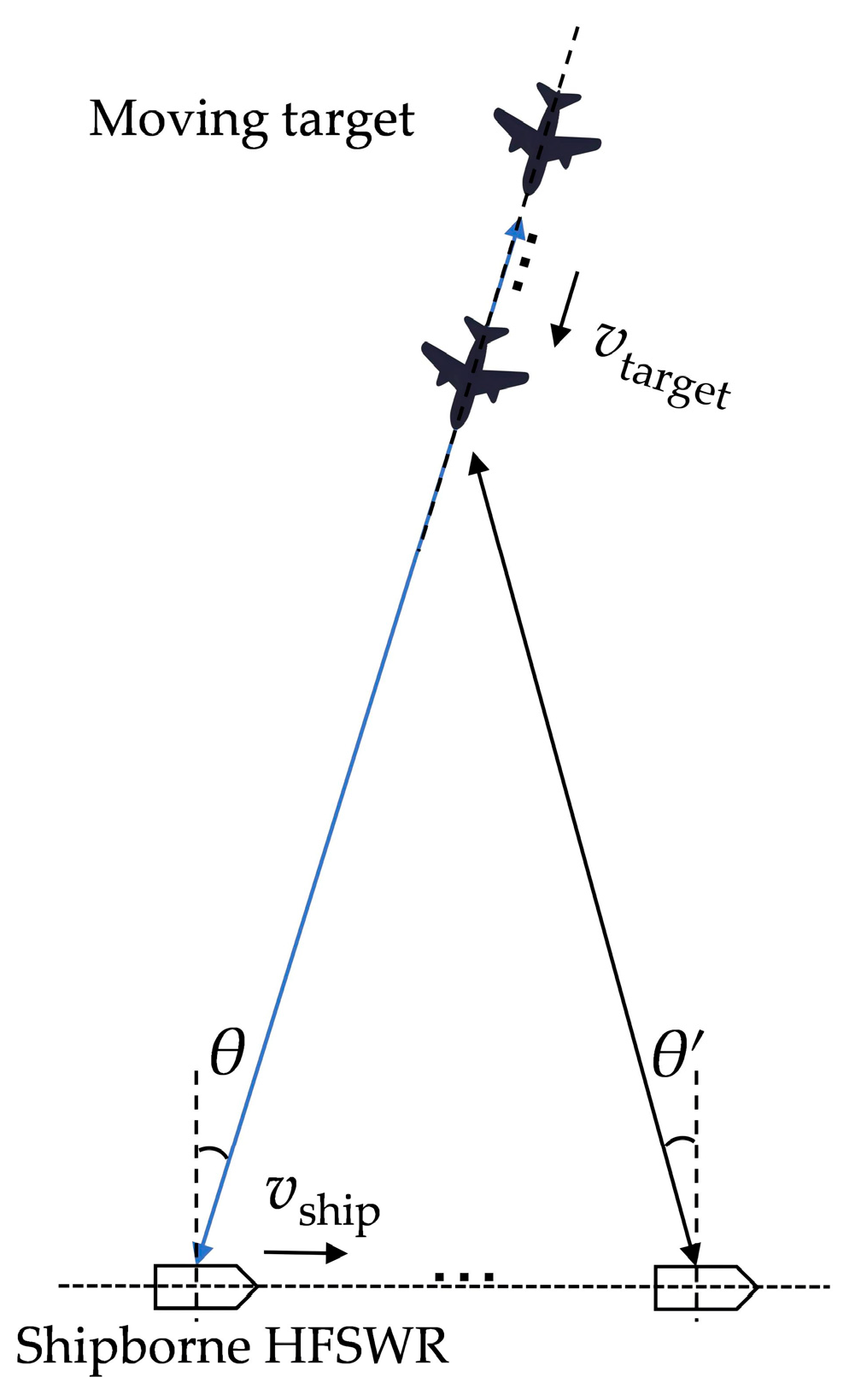
3.1. Far-Field Equivalent Motion Model

For the convenience of analyzing the proposed method, based on the far-field assumption in Section 2.1, we represent the motion model shown in Figure 1 equivalently to obtain the far-field equivalent motion model, as shown in Figure 2.

Figure 2. Far-field equivalent motion model for the shipborne HFSWR and moving target.

In Figure 2, the positions of the shipborne platform and target from time $t_0$ to ${(t}_0+\mathit{KT})$ are marked. Due to the far-field assumption, the target echo can be approximated as a plane wave. Therefore, for simplicity in analysis, we use the blue solid lines to represent the different positions of the far-field target. During the virtual aperture processing time $\mathit{KT}$, for each array element, we segment the received data by intervals $T$ to obtain $K$ time segments.

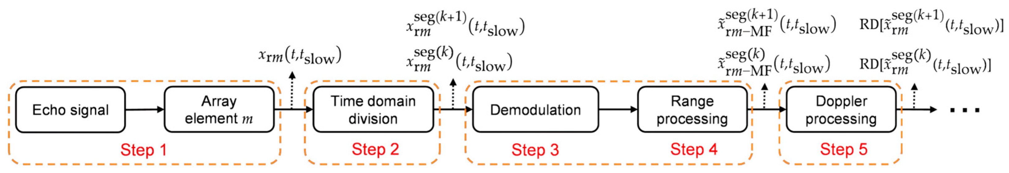
3.2. Flowchart of the Proposed Method

On the basis of conventional HFSWR processing flow, the flowchart of the proposed method (indicated by black dashed rectangular boxes) is shown in Figure 3.

Figure 3. Flowchart of the RD-domain virtual aperture extension method for shipborne HFSWR.

In conjunction with Figure 2, a brief explanation of the proposed flowchart is provided below. During the virtual aperture processing time KT, if the demodulated target echo signals from each array element are divided into $K$ time segments with a time interval $T$ (the order of demodulation and time–domain division can be interchanged), $M$ array elements will have a total of $M\cdot K$ time segments. For each time segment, we perform RD processing and target detection to obtain target’s $M$ snapshots of the real array (assume that targets are within a single RD unit). Then, we perform virtual aperture processing on $M\cdot K$ snapshots to obtain the target’s $M_{\mathrm{extend}}$ $(M_{\mathrm{extend}}>M)$ snapshots of the extended array. Finally, we use $M_{\mathrm{extend}}$ snapshots for DOA estimation to obtain target azimuth.

3.3. Signal Time–Domain Segmentation Model

This section provides the time–domain segmented representation of the array received data in the proposed method. For clarity, we provide the correspondence between the proposed flowchart and formula parameters in Figure 4 (the order of Step 2 and Step 3 can be exchanged). The explanation for Figure 4 is as follows.

Figure 4. The correspondence between the proposed flowchart and formula parameters.

Taking $N$ targets as an example and ignoring noise terms, the received data of element $m$ are represented as (8) (Step 1). Performing time domain division (Step 2) and the target echo received by element $m$ in time segment $k (k=1, 2, ..., K)$ and $(k+1)$ are represented as $x_{\mathrm{r}m}^{\mathrm{seg}(k)}\left(t,t_{\mathrm{slow}}\right)$ and $x_{\mathrm{r}m}^{\mathrm{seg}(k+1)}\left(t,t_{\mathrm{slow}}\right)$, respectively, as shown in (14) and (15).

$$\begin{array}{ll}{x}_{\mathrm{r}m}^{\mathrm{seg}(k)}\left(t,t_{\mathrm{slow}}\right)& ={\displaystyle \sum _{i=1}^N}{s}_{\mathrm{r}i}^{\mathrm{seg}(k)}\left(t,t_{\mathrm{slow}}\right)\cdot \exp \left[\mathrm{j}2\mathsf{\pi }{f}_{\mathrm{c}}{\displaystyle \frac{\left(m-1\right)d\sin {\theta }_i}{\mathrm{c}}}\right]\\ & ={\displaystyle \sum _{i=1}^N}s\left[t-{\displaystyle \frac{2R_i^{\mathrm{seg}(k)}\left(t_{\mathrm{slow}}\right)}{\mathrm{c}}}\right]\cdot \exp \left[\mathrm{j}2\mathsf{\pi }{f}_{\mathrm{c}}{\displaystyle \frac{\left(m-1\right)d\sin {\theta }_i}{\mathrm{c}}}\right]\end{array}$$

(14)

$$\begin{array}{ll}{x}_{\mathrm{r}m}^{\mathrm{seg}\left(k+1\right)}\left(t,t_{\mathrm{slow}}\right)& ={\displaystyle \sum _{i=1}^N}{s}_{\mathrm{r}i}^{\mathrm{seg}(k+1)}\left(t,t_{\mathrm{slow}}\right)\cdot \exp \left[\mathrm{j}2\mathsf{\pi }{f}_{\mathrm{c}}{\displaystyle \frac{\left(m-1\right)d\sin {\theta }_i}{\mathrm{c}}}\right]\\ & ={\displaystyle \sum _{i=1}^N}s\left[t-{\displaystyle \frac{2R_i^{\mathrm{seg}(k+1)}\left(t_{\mathrm{slow}}\right)}{\mathrm{c}}}\right]\cdot \exp \left[\mathrm{j}2\mathsf{\pi }{f}_{\mathrm{c}}{\displaystyle \frac{\left(m-1\right)d\sin {\theta }_i}{\mathrm{c}}}\right]\\ & ={\displaystyle \sum _{i=1}^N}s\left[t-{\displaystyle \frac{2R_i^{\mathrm{seg}(k)}\left(t_{\mathrm{slow}}\right)}{\mathrm{c}}}+{\displaystyle \frac{2\left(v_{\mathrm{ship}}\sin {\theta }_i+v_{\mathrm{target}i}\right)·T}{\mathrm{c}}}\right]\cdot \exp \left[\mathrm{j}2\mathsf{\pi }{f}_{\mathrm{c}}{\displaystyle \frac{\left(m-1\right)d\sin {\theta }_i}{\mathrm{c}}}\right]\end{array}$$

(15)

Here, $R_i^{\mathrm{seg}(k)}\left(t_{\mathrm{slow}}\right)$ and $R_i^{\mathrm{seg}(k+1)}\left(t_{\mathrm{slow}}\right)$, given by (16), respectively, represent the relative range of target $i$ that varies with $t_{\mathrm{slow}}$ during time segments $k$ and $(k+1)$. $s_{\mathrm{r}i}^{\mathrm{seg}(k)}\left(t,t_{\mathrm{slow}}\right)$ and $s_{\mathrm{r}i}^{\mathrm{seg}(k+1)}\left(t,t_{\mathrm{slow}}\right)$ represent the echo signal of target $i$ during time segments $k$ and $(k+1)$. $t_{\mathrm{slow}}$ is given by (5), where $\mathit{prtIndex}=0, 1, 2, \dots ,T/\mathit{PRT} (\mathrm{where} T/\mathit{PRT}\in \mathbb{N})$. The other parameters are the same as those in (8).

$$\begin{array}{l}\left\{\begin{array}{l}{R}_i^{\mathrm{seg}(k)}\left(t_{\mathrm{slow}}\right)=R_i-\left(v_{\mathrm{ship}}\sin {\theta }_i+v_{\mathrm{target}i}\right)\cdot \left(k-1\right)T-\left(v_{\mathrm{ship}}\sin {\theta }_i+v_{\mathrm{target}i}\right)\cdot t_{\mathrm{slow}}\\ R_i^{\mathrm{seg}(k+1)}\left(t_{\mathrm{slow}}\right)=R_i^{\mathrm{seg}(k)}\left(t_{\mathrm{slow}}\right)-\left(v_{\mathrm{ship}}\sin {\theta }_i+v_{\mathrm{target}i}\right)\cdot T\end{array}\right.\end{array}$$

(16)

According to Equation (11), demodulation and range processing (Step 3 and Step 4) are performed on (14) and (15), respectively, to obtain (17) and (18), as follows:

$$\begin{array}{ll}{\tilde{x}}_{\mathrm{r}m\text{-}\mathrm{MF}}^{\mathrm{seg}(k)}\left(t,t_{\mathrm{slow}}\right)=& {\displaystyle \sum _{i=1}^N}{\tilde{s}}_{\mathrm{r}i\text{-}\mathrm{MF}}^{\mathrm{seg}(k)}\left(t,t_{\mathrm{slow}}\right)\cdot \exp \left[\mathrm{j}2\mathsf{\pi }{f}_{\mathrm{c}}{\displaystyle \frac{\left(m-1\right)d\sin {\theta }_i}{\mathrm{c}}}\right]\\ & ={\displaystyle \sum _{i=1}^N}{\tau }_{\mathrm{p}}\sin \mathrm{c}\left\{B\left[t-{\displaystyle \frac{2R_i^{\mathrm{seg}(k)}\left(t_{\mathrm{slow}}\right)}{\mathrm{c}}}\right]\right\}\cdot \exp \left[-\mathrm{j}2\mathsf{\pi }{f}_{\mathrm{c}}{\displaystyle \frac{2R_i^{\mathrm{seg}(k)}\left(t_{\mathrm{slow}}\right)}{\mathrm{c}}}\right]\cdot \exp \left[\mathrm{j}2\mathsf{\pi }{f}_{\mathrm{c}}{\displaystyle \frac{\left(m-1\right)d\sin {\theta }_i}{\mathrm{c}}}\right]\end{array}$$

(17)

$$\begin{array}{ll}{\tilde{x}}_{\mathrm{r}m\text{-}\mathrm{MF}}^{\mathrm{seg}\left(k+1\right)}\left(t,t_{\mathrm{slow}}\right)& ={\displaystyle \sum _{i=1}^N}{\tilde{s}}_{\mathrm{r}i\text{-}\mathrm{MF}}^{\mathrm{seg}\left(k+1\right)}\left(t,t_{\mathrm{slow}}\right)\cdot \exp \left[\mathrm{j}2\mathsf{\pi }{f}_{\mathrm{c}}{\displaystyle \frac{\left(m-1\right)d\sin {\theta }_i}{\mathrm{c}}}\right]\\ & ={\displaystyle \sum _{i=1}^N}{\tau }_{\mathrm{p}}\sin \mathrm{c}\left\{B\left[t-{\displaystyle \frac{2R_i^{\mathrm{seg}(k+1)}\left(t_{\mathrm{slow}}\right)}{\mathrm{c}}}\right]\right\}\cdot \exp \left[-\mathrm{j}2\mathsf{\pi }{f}_{\mathrm{c}}{\displaystyle \frac{2R_i^{\mathrm{seg}(k+1)}\left(t_{\mathrm{slow}}\right)}{\mathrm{c}}}\right]\cdot \exp \left[\mathrm{j}2\mathsf{\pi }{f}_{\mathrm{c}}{\displaystyle \frac{\left(m-1\right)d\sin {\theta }_i}{\mathrm{c}}}\right]\\ & ={\displaystyle \sum _{i=1}^N}{\tau }_{\mathrm{p}}\sin \mathrm{c}\left\{B\left[t-{\displaystyle \frac{2R_i^{\mathrm{seg}(k)}\left(t_{\mathrm{slow}}\right)}{\mathrm{c}}}+\mathsf{\Delta }{\tau }_{\mathrm{ship}i}+\mathsf{\Delta }{\tau }_{\mathrm{target}i}\right]\right\}\cdot \exp \left[-\mathrm{j}2\mathsf{\pi }{f}_{\mathrm{c}}{\displaystyle \frac{2R_i^{\mathrm{seg}(k)}\left(t_{\mathrm{slow}}\right)}{\mathrm{c}}}\right]·\\ & \mathrm{e}\mathrm{x}\mathrm{p}\left[\mathrm{j}2\mathsf{\pi }{f}_{\mathrm{c}}{\displaystyle \frac{\left(m-1\right)d\sin {\theta }_i}{\mathrm{c}}}\right]\cdot \mathrm{e}\mathrm{x}\mathrm{p}\left(\mathrm{j}2\mathsf{\pi }{f}_{\mathrm{c}}\mathsf{\Delta }{\tau }_{\mathrm{ship}i}\right)\cdot \mathrm{e}\mathrm{x}\mathrm{p}\left(\mathrm{j}2\mathsf{\pi }{f}_{\mathrm{c}}\mathsf{\Delta }{\tau }_{\mathrm{target}i}\right)\end{array}$$

(18)

where $\mathsf{\Delta }{\tau }_{\mathrm{ship}i}$ and $\mathsf{\Delta }{\tau }_{\mathrm{target}i}$ represent the changes in echo delay of target $i$ caused by the motion of ship and target $i$ during time $T$, respectively, as shown in (19).

$$\left\{\begin{array}{l}\mathsf{\Delta }{\tau }_{\mathrm{ship}i}=2v_{\mathrm{ship}}\sin {\theta }_i\cdot T/\mathrm{c}\\ \mathsf{\Delta }{\tau }_{\mathrm{target}i}={2v}_{\mathrm{target}i}\cdot T/\mathrm{c}\end{array}\right.$$

(19)

Step 5 represents for the Doppler processing and its output in time segment $k$ and $(k+1)$ are represented as $\mathrm{RD}[{\tilde{x}}_{\mathrm{r}m}^{\mathrm{seg}(k)}(t,t_{\mathrm{slow}}\left)\right]$ and $\mathrm{RD}[{\tilde{x}}_{\mathrm{r}m}^{\mathrm{seg}(k+1)}(t,t_{\mathrm{slow}}\left)\right]$.

3.4. Proposed Method for a Single Target

This section derives the proposed RD-domain virtual aperture extension method for a single target. Before introducing the method, we first provide an RD-domain representation of the array received data. By applying the RD processing to (6) and utilizing the linear properties of the RD transformation, we obtain

$$\mathrm{R}{\mathrm{D}}_{\mathit{ij}}[x_{\mathrm{r}m}(t\left)\right]={\displaystyle \sum _{i=1}^N}\mathrm{R}{\mathrm{D}}_{\mathit{ij}}[s_{\mathrm{r}i}\left(t\right)]\cdot \exp \left[\mathrm{j}2\mathsf{\pi }{f}_{\mathrm{c}}{\displaystyle \frac{\left(m-1\right)d\sin {\theta }_i}{\mathrm{c}}}\right]+\mathrm{R}{\mathrm{D}}_{\mathit{ij}}[n_m(t\left)\right]$$

(20)

Then, the RD-domain representation of array data can be obtained, as shown in (21), as follows:

$$\left[\begin{array}{c}\mathrm{R}{\mathrm{D}}_{\mathit{ij}}\left[x_{\mathrm{r}1}\right(t\left)\right]\\ \mathrm{R}{\mathrm{D}}_{\mathit{ij}}\left[x_{\mathrm{r}2}\right(t\left)\right]\\ ⋮\\ \mathrm{R}{\mathrm{D}}_{\mathit{ij}}\left[x_{\mathrm{r}M}\right(t\left)\right]\end{array}\right]=\mathbf{A}·\left[\begin{array}{c}\mathrm{R}{\mathrm{D}}_{\mathit{ij}}\left[s_{\mathrm{r}1}\right(t\left)\right]\\ \mathrm{R}{\mathrm{D}}_{\mathit{ij}}\left[s_{\mathrm{r}2}\right(t\left)\right]\\ ⋮\\ \mathrm{R}{\mathrm{D}}_{\mathit{ij}}\left[s_{\mathrm{r}N}\right(t\left)\right]\end{array}\right]+\left[\begin{array}{c}\mathrm{R}{\mathrm{D}}_{\mathit{ij}}\left[n_1\right(t\left)\right]\\ \mathrm{R}{\mathrm{D}}_{\mathit{ij}}\left[n_2\right(t\left)\right]\\ ⋮\\ \mathrm{R}{\mathrm{D}}_{\mathit{ij}}\left[n_M\right(t\left)\right]\end{array}\right]$$

(21)

where $\mathrm{R}{\mathrm{D}}_{\mathit{ij}}\left[x_{\mathrm{r}m}\right(t\left)\right]$ represents the single snapshot value of range index $i$ and the velocity index $j$ is extracted from the RD-processed data of element $m$.

Based on the flowchart shown in Figure 3, the proposed method is explained as follows.

Firstly, for the received data of each array element, we perform demodulation and time–domain division (as described in Section 3.3) to obtain the baseband data of array element m in time segment k, denoted as ${\tilde{x}}_{\mathrm{r}m}^{\mathrm{seg}(k)}(t)$.

Secondly, RD processing is performed on ${\tilde{x}}_{\mathrm{r}m}^{\mathrm{seg}(k)}(t)$. According to (21), for a single target, the RD-domain form of the array data in time segment $k$ is expressed as

$$\left[\begin{array}{c}\mathrm{R}\mathrm{D}[{\tilde{x}}_{\mathrm{r}1}^{\mathrm{seg}(k)}(t)]\\ \mathrm{R}\mathrm{D}[{\tilde{x}}_{\mathrm{r}2}^{\mathrm{seg}(k)}(t)]\\ ⋮\\ \mathrm{R}\mathrm{D}[{\tilde{x}}_{\mathrm{r}M}^{\mathrm{seg}(k)}(t)]\end{array}\right]={\mathit{a}}_1·\mathrm{RD}[{\tilde{s}}_{\mathrm{r}1}^{\mathrm{seg}(k)}(t)]+\left[\begin{array}{c}\mathrm{R}\mathrm{D}[n_1^{\mathrm{seg}(k)}(t)]\\ \mathrm{R}\mathrm{D}[n_2^{\mathrm{seg}(k)}(t)]\\ ⋮\\ \mathrm{R}\mathrm{D}[n_M^{\mathrm{seg}(k)}(t)]\end{array}\right]$$

(22)

where ${\tilde{s}}_{\mathrm{r}1}^{\mathrm{seg}(k)}(t)$ represents the baseband target signal in time segment k.

Thirdly, through target detection, we obtain the targets’ range and velocity indices $\mathit{ij}$ of the RD spectrum and extract the targets’ single-snapshot value at indices $\mathit{ij}$. Similar to (21), the value of indices ij are denoted as $\mathrm{R}{\mathrm{D}}_{\mathit{ij}}\left[{\tilde{x}}_{\mathrm{r}m}^{\mathrm{seg}(k)}\left(t\right)\right]$, $\mathrm{R}{\mathrm{D}}_{\mathit{ij}}\left[{\tilde{s}}_{\mathrm{r}1}^{\mathrm{seg}(k)}\left(t\right)\right]$, and $\mathrm{R}{\mathrm{D}}_{\mathit{ij}}\left[n_m^{\mathrm{seg}(k)}\left(t\right)\right]$. For the convenience of formula derivation, we represent them as $x_{\mathrm{r}m}^{\mathrm{seg}(k)}$, $s_{\mathrm{r}1}^{\mathrm{seg}(k)}$, and $n_m^{\mathrm{seg}(k)}$, respectively. Substituting (7) into (22) yields (23).

$$\left[\begin{array}{c}{x}_{\mathrm{r}1}^{\mathrm{seg}(k)}\\ x_{\mathrm{r}2}^{\mathrm{seg}(k)}\\ ⋮\\ x_{\mathrm{r}M}^{\mathrm{seg}(k)}\end{array}\right]=\left[\begin{array}{c}{\mathrm{e}}^{\mathrm{j}2\mathsf{\pi }{f}_{\mathrm{c}}{\displaystyle \frac{0·d\sin {\theta }_1}{\mathrm{c}}}}\\ {\mathrm{e}}^{\mathrm{j}2\mathsf{\pi }{f}_{\mathrm{c}}{\displaystyle \frac{1·d\sin {\theta }_1}{\mathrm{c}}}}\\ ⋮\\ {\mathrm{e}}^{\mathrm{j}2\mathsf{\pi }{f}_{\mathrm{c}}{\displaystyle \frac{\left(M-1\right)·d\sin {\theta }_1}{\mathrm{c}}}}\end{array}\right]\cdot s_{\mathrm{r}1}^{\mathrm{seg}(k)}+\left[\begin{array}{c}{n}_1^{\mathrm{seg}(k)}\\ n_2^{\mathrm{seg}(k)}\\ ⋮\\ n_M^{\mathrm{seg}(k)}\end{array}\right]$$

(23)

Similarly, the RD-domain representation of the array data for time segment $(k+1)$ is given by (24).

$$\left[\begin{array}{c}{x}_{\mathrm{r}1}^{\mathrm{seg}(k+1)}\\ x_{\mathrm{r}2}^{\mathrm{seg}(k+1)}\\ ⋮\\ x_{\mathrm{r}M}^{\mathrm{seg}(k+1)}\end{array}\right]=\left[\begin{array}{c}{\mathrm{e}}^{\mathrm{j}2\mathsf{\pi }{f}_{\mathrm{c}}{\displaystyle \frac{0·d\sin {\theta }_1}{\mathrm{c}}}}\\ {\mathrm{e}}^{\mathrm{j}2\mathsf{\pi }{f}_{\mathrm{c}}{\displaystyle \frac{1·d\sin {\theta }_1}{\mathrm{c}}}}\\ ⋮\\ {\mathrm{e}}^{\mathrm{j}2\mathsf{\pi }{f}_{\mathrm{c}}{\displaystyle \frac{\left(M-1\right)·d\sin {\theta }_1}{\mathrm{c}}}}\end{array}\right]\cdot s_{\mathrm{r}1}^{\mathrm{seg}(k+1)}+\left[\begin{array}{c}{n}_1^{\mathrm{seg}(k+1)}\\ n_2^{\mathrm{seg}(k+1)}\\ ⋮\\ n_M^{\mathrm{seg}(k+1)}\end{array}\right]$$

(24)

Fourthly, based on the real-array elements’ M snapshots of each time segments, we perform virtual aperture processing to obtain the extended-array elements’ $M_{\mathrm{extend}}$ snapshots. If the SNR is high enough after RD processing, the noise terms in (23) and (24) can be neglected, and dividing Equation (24) by Equation (23) results in

$${\mathsf{\Delta }\phi }_m=\begin{array}{l}{\displaystyle \frac{x_{\mathrm{r}m}^{\mathrm{seg}(k+1)}}{x_{\mathrm{r}{m}^{\prime }}^{\mathrm{seg}(k)}}}={\displaystyle \frac{\exp \left(\mathrm{j}2\mathsf{\pi }{f}_{\mathrm{c}}\frac{\left(m-1\right)\cdot d\sin {\theta }_1}{\mathrm{c}}\right)\cdot s_{\mathrm{r}1}^{\mathrm{seg}(k+1)}}{\exp \left(\mathrm{j}2\mathsf{\pi }{f}_{\mathrm{c}}\frac{\left(m^{\prime }-1\right)\cdot d\sin {\theta }_1}{\mathrm{c}}\right)\cdot s_{\mathrm{r}1}^{\mathrm{seg}(k)}}}={\displaystyle \frac{x_{\mathrm{r}(m+1)}^{\mathrm{seg}(k+1)}}{x_{\mathrm{r}(m^{\prime }+1)}^{\mathrm{seg}(k)}}}\end{array}$$

(25)

Here, $m^{\prime }$ and $m$ represent the element indices in time segment $k$ and $\left(k+1\right),$ respectively, which satisfy $1\le m<m^{\prime }\le M$. $x_{\mathrm{r}{m}^{\prime }}^{\mathrm{seg}(k)}$ represents the extracted target single snapshot of element $m^{\prime }$ in time segment $k$, $x_{\mathrm{r}m}^{\mathrm{seg}(k+1)}$ represents the extracted target single snapshot of element $m$ in time segment $(k+1)$, and ${\mathsf{\Delta }\phi }_m$ represents the compensation value between the two single snapshots.

If the index difference $\mathsf{\Delta }m$ is denoted as $\mathsf{\Delta }m=m^{\prime }-m$ and satisfies $1\le \mathsf{\Delta }m\le M-1$, then (25) can also be expressed as

$$\begin{array}{l}{\mathsf{\Delta }\phi }_m={\displaystyle \frac{x_{\mathrm{r}m}^{\mathrm{seg}(k+1)}}{x_{\mathrm{r}(m+\mathsf{\Delta }m)}^{\mathrm{seg}(k)}}}={\displaystyle \frac{\exp \left(\mathrm{j}2\mathsf{\pi }{f}_{\mathrm{c}}\frac{\left(m-1\right)·d\sin {\theta }_1}{\mathrm{c}}\right)\cdot s_{\mathrm{r}1}^{\mathrm{seg}(k+1)}}{\exp \left(\mathrm{j}2\mathsf{\pi }{f}_{\mathrm{c}}\frac{\left(m+\mathsf{\Delta }m-1\right)·d\sin {\theta }_1}{\mathrm{c}}\right)\cdot s_{\mathrm{r}1}^{\mathrm{seg}(k)}}}={\displaystyle \frac{x_{\mathrm{r}(m+1)}^{\mathrm{seg}(k+1)}}{x_{\mathrm{r}(m+\mathsf{\Delta }m+1)}^{\mathrm{seg}(k)}}}{=\mathsf{\Delta }\phi }_{(m+1)}\end{array}$$

(26)

Due to the potential data errors in a single array element, we take the average of ${\mathsf{\Delta }\phi }_m$ to obtain $\overline{{\mathsf{\Delta }\phi }_m}$ in (27), which represents the average compensation value between time segment $k$ and $(k+1)$.

$$\overline{{\mathsf{\Delta }\phi }_m}=\mathrm{E}\left({\mathsf{\Delta }\phi }_m\right)={\displaystyle \frac{1}{(M-\mathsf{\Delta }m)}}{\displaystyle \sum _{m=1}^{M-\mathsf{\Delta }m}}{\displaystyle \frac{x_{\mathrm{r}m}^{\mathrm{seg}(k+1)}}{x_{\mathrm{r}(m+\mathsf{\Delta }m)}^{\mathrm{seg}(k)}}}$$

(27)

Then, the virtual elements’ single-snapshot data $x_{\mathrm{r}\left(M+1\right)}^{\mathrm{seg}(k)}$ to $x_{\mathrm{r}(M+\mathsf{\Delta }m)}^{\mathrm{seg}(k)}$ can be calculated from

$${\displaystyle \frac{x_{\mathrm{r}\left(M+1-\mathsf{\Delta }m\right)}^{\mathrm{seg}(k+1)}}{x_{\mathrm{r}\left(M+1\right)}^{\mathrm{seg}(k)}}}=\cdots ={\displaystyle \frac{x_{\mathrm{r}M}^{\mathrm{seg}(k+1)}}{x_{\mathrm{r}(M+\mathsf{\Delta }m)}^{\mathrm{seg}(k)}}}=\overline{{\mathsf{\Delta }\phi }_m}$$

(28)

By traversing the values of $k$ from 1 to $K$, $\mathsf{\Delta }m\cdot (K-1)$ extended elements’ single-snapshot data can be obtained in time segment 1, that is, the number of the extended array elements is $M_{\mathrm{extend}}$, which satisfies the condition $M_{\mathrm{extend}}=M+\mathsf{\Delta }m\cdot (K-1)$.

Finally, based on the target’s $M_{\mathrm{extend}}$ snapshots of the extended array, we perform DOA estimation to obtain the target azimuth.

The virtual aperture processing method and aperture expansion effect of the proposed method are shown in Figure 5.

Figure 5. Virtual aperture processing method and aperture expansion effect of the proposed method for a single target. (a) Virtual aperture processing method. (b) Aperture expansion effect when $\mathsf{\Delta }m=1$. (c) Aperture expansion effect when $\mathsf{\Delta }m=M-1$.

Figure 5a shows the virtual aperture processing manners of the proposed method. The dashed arrows correspond to different $\mathsf{\Delta }m$ ($1\le \mathsf{\Delta }m\le M-1$), where the blue dashed arrow represents $\mathsf{\Delta }m=1$, the red dashed arrow represents $\mathsf{\Delta }m=2$, and the green dashed arrow represents $\mathsf{\Delta }m=M-1$. Figure 5b shows the aperture expansion effect when $\mathsf{\Delta }m=1$. In this case, only one virtual element’s single-snapshot data can be obtained after a single virtual aperture processing, representing the minimum aperture case. Figure 5c shows the aperture expansion effect when $\mathsf{\Delta }m=M-1$. In this case, $(M-1)$ virtual elements’ single-snapshot data can be obtained after a single virtual aperture processing, which represents the maximum aperture case. However, this does not imply that a larger $\mathsf{\Delta }m$ is always better. For example, when $\mathsf{\Delta }m=M-1$, according to (27), $\overline{{\mathsf{\Delta }\phi }_m}$ is calculated from only a pair of elements’ data $x_{\mathrm{r}1}^{\mathrm{seg}(k+1)}$ and $x_{\mathrm{r}M}^{\mathrm{seg}(k)}$, which means that the value of $\overline{{\mathsf{\Delta }\phi }_m}$ is more susceptible to noise and may have potential errors.

Additionally, it should be noted that the derivation of the proposed method is based on a uniform linear array. For the case of non-uniform linear arrays, ${\mathsf{\Delta }\phi }_m{=\mathsf{\Delta }\phi }_{(m+1)}$ in equation (26) cannot be derived and the proposed method is no longer applicable.

3.5. Proposed Method for Multiple Targets

This section derives the proposed RD-domain virtual aperture extension method for multiple targets.

When multiple targets are present, two cases are considered: the first case is when all targets are situated in different RD units and the second case is when at least two targets are situated in the same RD unit.

For case 1, we can apply the RD-domain virtual aperture extension method described in Section 3.4 to each individual target of different RD units, to achieve the virtual aperture extension.

For case 2, the processing flow of the method is consistent with that in Section 3.4; however, two constraints are present: the first is that the array needs to move in an overlapping manner, which means it satisfies the condition $v_{\mathrm{ship}}T=\mathit{ld}$ (where $\mathit{l}=1, 2, \dots , M-1$), and the second is that $\mathsf{\Delta }m$ must meet the requirement $\mathsf{\Delta }m=2\mathit{l}$.

The explanation of the two constraints in case 2 is as follows. According to (18), when the target speed is low or the virtual aperture processing time is short, the impact of $\mathsf{\Delta }{\tau }_{\mathrm{ship}i}$ and $\mathsf{\Delta }{\tau }_{\mathrm{target}i}$ on the envelope of the $\sin \mathrm{c}$ function can be ignored, resulting in (29), with the parameters specified in (16) and (19).

$$\begin{array}{ll}{\tilde{x}}_{\mathrm{r}m\text{-}\mathrm{MF}}^{\mathrm{seg}\left(k+1\right)}\left(t,t_{\mathrm{slow}}\right)& ={\displaystyle \sum _{i=1}^N}{\tau }_{\mathrm{p}}\sin \mathrm{c}[B(t-{\displaystyle \frac{2R_i^{\mathrm{seg}(k)}\left(t_{\mathrm{slow}}\right)}{\mathrm{c}}}\left)\right]\cdot \exp \left[-\mathrm{j}2\mathsf{\pi }{f}_{\mathrm{c}}{\displaystyle \frac{2R_i^{\mathrm{seg}(k+1)}\left(t_{\mathrm{slow}}\right)}{\mathrm{c}}}\right]\cdot \exp \left[\mathrm{j}2\mathsf{\pi }{f}_{\mathrm{c}}{\displaystyle \frac{\left(m-1\right)d\sin {\theta }_i}{\mathrm{c}}}\right]\\ & ={\displaystyle \sum _{i=1}^N}{\tau }_{\mathrm{p}}\sin \mathrm{c}[B(t-{\displaystyle \frac{2R_i^{\mathrm{seg}(k)}\left(t_{\mathrm{slow}}\right)}{\mathrm{c}}}\left)\right]\cdot \exp \left[-\mathrm{j}2\mathsf{\pi }{f}_{\mathrm{c}}{\displaystyle \frac{2R_i^{\mathrm{seg}(k)}\left(t_{\mathrm{slow}}\right)}{\mathrm{c}}}\right]\cdot \mathrm{e}\mathrm{x}\mathrm{p}\left[\mathrm{j}2\mathsf{\pi }{f}_{\mathrm{c}}{\displaystyle \frac{\left(m-1\right)d\sin {\theta }_i}{\mathrm{c}}}\right]\cdot \\ & \mathrm{e}\mathrm{x}\mathrm{p}\left(\mathrm{j}2\mathsf{\pi }{f}_{\mathrm{c}}\mathsf{\Delta }{\tau }_{\mathrm{ship}i}\right)\cdot \mathrm{e}\mathrm{x}\mathrm{p}\left(\mathrm{j}2\mathsf{\pi }{f}_{\mathrm{c}}\mathsf{\Delta }{\tau }_{\mathrm{target}i}\right)\end{array}$$

(29)

Given that targets are in the same RD unit, we assume that their range and velocity parameters are exactly the same. We assume that the array moves in an overlapping manner, which means that constraint 1 holds. Taking $l$ = 1 as an example, substituting $v_{\mathrm{target}i}=v_{\mathrm{target}}$, $R_i=R$ and $v_{\mathrm{ship}}T=d$ into (29) yields

$$\begin{array}{ll}{\tilde{x}}_{\mathrm{r}m\text{-}\mathrm{MF}}^{\mathrm{seg}\left(k+1\right)}\left(t,t_{\mathrm{slow}}\right)& ={\displaystyle \sum _{i=1}^N}{\tau }_{\mathrm{p}}\sin \mathrm{c}[B(t-{\displaystyle \frac{2R_i^{\mathrm{seg}(k)}\left(t_{\mathrm{slow}}\right)}{\mathrm{c}}}\left)\right]\cdot \exp \left[-\mathrm{j}2\mathsf{\pi }{f}_{\mathrm{c}}{\displaystyle \frac{2R_i^{\mathrm{seg}(k)}\left(t_{\mathrm{slow}}\right)}{\mathrm{c}}}\right]·\\ & \mathrm{e}\mathrm{x}\mathrm{p}\left[\mathrm{j}2\mathsf{\pi }{f}_{\mathrm{c}}{\displaystyle \frac{\left(m+1\right)d\sin {\theta }_i}{\mathrm{c}}}\right]\cdot \mathrm{e}\mathrm{x}\mathrm{p}(\mathrm{j}2\mathsf{\pi }{f}_{\mathrm{c}}\mathsf{\Delta }{\tau }_{\mathrm{target}})\\ & ={\tilde{x}}_{\mathrm{r}(m+2)\text{-}\mathrm{MF}}^{\mathrm{seg}(k)}\left(t,t_{\mathrm{slow}}\right)\cdot \mathrm{e}\mathrm{x}\mathrm{p}\left(\mathrm{j}2\mathsf{\pi }{f}_{\mathrm{c}}\mathsf{\Delta }{\tau }_{\mathrm{target}}\right)\end{array}$$

(30)

where $R_i^{\mathrm{seg}(k)}\left(t_{\mathrm{slow}}\right)=R-\left(v_{\mathrm{ship}}\sin {\theta }_i+v_{\mathrm{target}}\right)\cdot \left(k-1\right)T-\left(v_{\mathrm{ship}}\sin {\theta }_i+v_{\mathrm{target}}\right)\cdot t_{\mathrm{slow}}$ and $\mathsf{\Delta }{\tau }_{\mathrm{target}}={2v}_{\mathrm{target} }\cdot T/\mathrm{c}$.

Simultaneously perform DFT on both sides of the Equation (30) with respect to $t_{\mathrm{slow}}$, resulting in

$$\begin{array}{ll}\mathrm{R}\mathrm{D}\left[{\tilde{x}}_{\mathrm{r}m}^{\mathrm{seg}\left(k+1\right)}\left(t,t_{\mathrm{slow}}\right)\right]& ={\mathrm{DFT}}_{t_{\mathrm{slow}}}\left[{\tilde{x}}_{\mathrm{r}m\text{-}\mathrm{MF}}^{\mathrm{seg}\left(k+1\right)}\left(t,t_{\mathrm{slow}}\right)\right]\\ & ={\mathrm{DFT}}_{t_{\mathrm{slow}}}\left[{\tilde{x}}_{\mathrm{r}(m+2)\text{-}\mathrm{MF}}^{\mathrm{seg}(k)}\left(t,t_{\mathrm{slow}}\right)\right]\cdot \exp \left(\mathrm{j}2\mathsf{\pi }{f}_{\mathrm{c}}\mathsf{\Delta }{\tau }_{\mathrm{target}}\right)\\ & =\mathrm{R}\mathrm{D}\left[{\tilde{x}}_{\mathrm{r}(m+2)}^{\mathrm{seg}(k)}\left(t,t_{\mathrm{slow}}\right)\right]\cdot \exp \left(\mathrm{j}2\mathsf{\pi }{f}_{\mathrm{c}}\mathsf{\Delta }{\tau }_{\mathrm{target}}\right)\end{array}$$

(31)

Similar to Section 3.4, extract the single-snapshot value at indices $\mathit{ij}$ from (31) to obtain ${\mathrm{RD}}_{\mathit{ij}}\left[{\tilde{x}}_{\mathrm{r}m}^{\mathrm{seg}\left(k+1\right)}\left(t,t_{\mathrm{slow}}\right)\right]$ and ${\mathrm{RD}}_{\mathit{ij}}\left[{\tilde{x}}_{\mathrm{r}(m+2)}^{\mathrm{seg}(k)}\left(t,t_{\mathrm{slow}}\right)\right]$ and denote them as $x_{\mathrm{r}m}^{\mathrm{seg}\left(k+1\right)}$ and $x_{\mathrm{r}(m+2)}^{\mathrm{seg}(k)}$, respectively, resulting in

$$\begin{array}{l}{\mathsf{\Delta }\phi }_m={\displaystyle \frac{x_{\mathrm{r}m}^{\mathrm{seg}\left(k+1\right)}}{{\mathrm{x}}_{\mathrm{r}(m+2)}^{\mathrm{seg}(k)}}}=\exp \left(\mathrm{j}2\mathsf{\pi }{f}_{\mathrm{c}}\mathsf{\Delta }{\tau }_{\mathrm{target}}\right)\end{array}={\mathsf{\Delta }\phi }_{(m+1)}$$

(32)

Compared to (26), it can be seen that $\mathsf{\Delta }m$ can only take 2 for multiple targets, which means that constraint 2 holds.

The same as for Equations (27) and (28), the virtual array elements’ data $x_{\mathrm{r}(M+1)}^{\mathrm{seg}(k)}$ and $x_{\mathrm{r}(M+2)}^{\mathrm{seg}(k)}$ can be calculated by (33). The elements number of the extended array is $M_{\mathrm{extend}}=M+2(K-1)$.

$$\overline{{\mathsf{\Delta }\phi }_m}=\mathrm{E}\left({\mathsf{\Delta }\phi }_m\right)={\displaystyle \frac{1}{(M-2)}}{\displaystyle \sum _{m=1}^{M-2}}{\displaystyle \frac{x_{\mathrm{r}m}^{\mathrm{seg}\left(k+1\right)}}{x_{\mathrm{r}(m+2)}^{\mathrm{seg}(k)}}}={\displaystyle \frac{x_{\mathrm{r}(M-1)}^{\mathrm{seg}\left(k+1\right)}}{x_{\mathrm{r}(M+1)}^{\mathrm{seg}(k)}}}={\displaystyle \frac{x_{\mathrm{r}M}^{\mathrm{seg}\left(k+1\right)}}{x_{\mathrm{r}(M+2)}^{\mathrm{seg}(k)}}}$$

(33)

Therefore, only when both constraints are satisfied can the phase compensation value between two elements across two time segments be expressed as the constant $\exp \left(\mathrm{j}2\mathsf{\pi }{f}_{\mathrm{c}}\mathsf{\Delta }{\tau }_{\mathrm{target}}\right)$. Then, the condition ${\mathsf{\Delta }\phi }_m={\mathsf{\Delta }\phi }_{(m+1)}$ is satisfied and the proposed method for multiple targets in case 2 becomes effective.

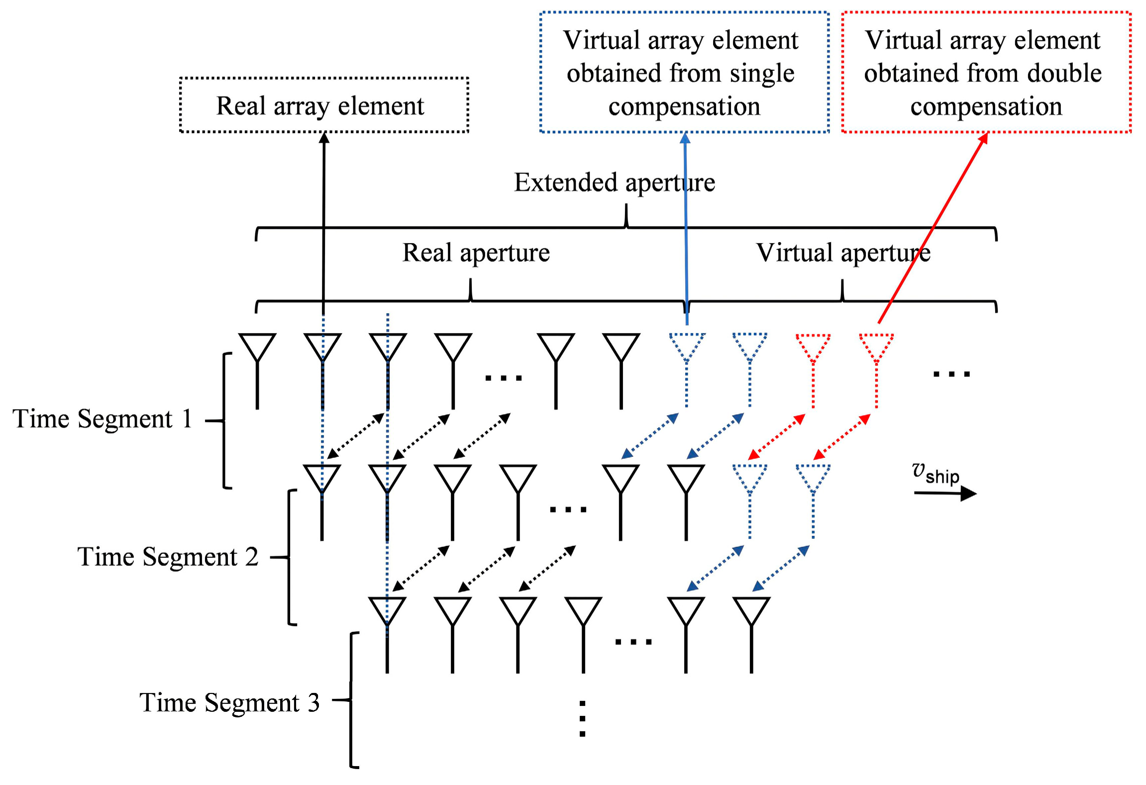
The virtual aperture processing method and aperture expansion effect of the proposed method for multiple targets when l = 1 is shown in Figure 6.

Figure 6. Virtual aperture processing method and aperture expansion effect of the proposed method for multiple targets when l = 1.

Here, the black solid-line element represents the element of the real array, the blue dashed-line element represents for the virtual array element obtained from a single virtual aperture processing, and the red dashed-line element represents for the virtual array element obtained from double virtual aperture processing.

It can be seen that the array element $m$ in time segment $\left(k+1\right)$ corresponds to the array element $(m+2)$ in time segment $k$. That is, two virtual elements’ data can be obtained from each virtual aperture processing of time $T$, indicating that the aperture extension performance is limited compared to the proposed method for a single target.

4. Performance Discussion

4.1. Aperture Extension Performance Based on a Far-Field Assumption

In this section, we analyze the factors influencing the far-field assumption to explain the limitations in the aperture extension performance of the proposed method.

According to Section 3.4, the elements number of the extended array is $M_{\mathrm{extend}}=M+\mathsf{\Delta }m\cdot (K-1)$. Under ideal conditions, if the far-field assumption mentioned in Section 2.1 is always satisfied, the virtual aperture can be infinitely large as the virtual aperture processing time $\mathit{KT}$ increases. However, in practice, due to various factors, the far-field assumption holds only within a certain range of parameters; therefore, the extension of the array aperture is limited.

To illustrate the factors that may influence the far-field assumption, we conduct simulations from two perspectives: the first is azimuth variation ($\mathsf{\Delta }\theta$) within the virtual aperture processing time and the second is elements’ maximum phase variation ($\mathsf{\Delta }{\varphi }_{\max }$), which represents the phase change in element M caused by $\mathsf{\Delta }\theta$ when element 1 is used as the reference element.

$$\mathsf{\Delta }\theta =\left|\theta -{\theta }^{\prime }\right|$$

(34)

$$\mathsf{\Delta }{\varphi }_{\max }={\displaystyle \frac{2\mathsf{\pi }}{\lambda }}\left(M-1\right)d\left[\sin \left({\theta }^{\prime }\right)-\sin \theta \right]$$

(35)

The parameter settings are as follows: $v_{\mathrm{ship}}$ is about 20 knots, $v_{\mathrm{target} }$ is about 1 Mach, the target range is from 30 km to 150 km, and the target azimuth $\theta \in \{0°,15°,30°\}$. For simplicity in analysis, we assume that the target moves toward the radar. Figure 7 illustrates the changes in $\mathsf{\Delta }\theta$ and $\mathsf{\Delta }{\varphi }_{\max }$ with respect to the target range, under the different target azimuths and virtual aperture processing times.

Figure 7. Analysis of the far-field assumption. (a) $\mathsf{\Delta }\theta$. (b) $\mathsf{\Delta }{\varphi }_{\max }$.

In Figure 7, the circle dotted lines represent a virtual aperture processing time of 5 s, and the upper triangular dotted lines represent a virtual aperture processing time of 10 s. The green, red, and blue lines represent the target azimuths of $0°, 15° \mathrm{and} 30°$, respectively.

It can be seen that within the given parameter range, the values of $\mathsf{\Delta }\theta$ and $\mathsf{\Delta }{\varphi }_{\max }$ are relatively small, which has little impact on DOA estimation, indicating that the far-field assumption is valid. However, as the virtual aperture processing time increases, $\mathsf{\Delta }\theta$ and $\mathsf{\Delta }{\varphi }_{\max }$ gradually increase. Additionally, as the target range or target azimuth decreases, $\mathsf{\Delta }\theta$ and $\mathsf{\Delta }{\varphi }_{\max }$ also increase. When $\mathsf{\Delta }\theta$ and $\mathsf{\Delta }{\varphi }_{\max }$ are relatively large, the far-field assumption no longer holds, and the proposed method may have significant errors or even fail. Therefore, the aperture extension performance of the proposed method is limited in practice.

4.2. Analysis of Error Impact

This section analyzes the potential errors of the proposed RD-domain virtual aperture extension method and their impact on the method.

To evaluate the impact of errors on the proposed virtual aperture processing method, we define the parameter $\mathrm{Var}(\widehat{{\mathsf{\Delta }\phi }_m})$, as shown in (36).

$$\mathrm{Var}\left(\widehat{{\mathsf{\Delta }\phi }_m}\right)={\displaystyle \frac{1}{(M-\mathsf{\Delta }m)}}{\displaystyle \sum _{m=1}^{M-\mathsf{\Delta }m}}{\left|\widehat{{\mathsf{\Delta }\phi }_m}-\mathrm{E}\left(\widehat{{\mathsf{\Delta }\phi }_m}\right)\right|}^2$$

(36)

where ${\mathsf{\Delta }\phi }_m$ is defined in (26) or (32) and $\widehat{{\mathsf{\Delta }\phi }_m}$ represents the estimated value of ${\mathsf{\Delta }\phi }_m$. E($\widehat{{\mathsf{\Delta }\phi }_m}$) and Var($\widehat{{\mathsf{\Delta }\phi }_m}$) represent the mean value and variance of $\widehat{{\mathsf{\Delta }\phi }_m}$, respectively.

The explanation of the parameter $\mathrm{Var}(\widehat{{\mathsf{\Delta }\phi }_m})$ is as follows. As shown in (27) and (33), the proposed method calculates the virtual elements’ data through $\overline{{\mathsf{\Delta }\phi }_m}$. In the absence of error, ${\mathsf{\Delta }\phi }_m$ does not vary with $m$, indicating that $\mathrm{Var}\left({\mathsf{\Delta }\phi }_m\right)=0$ and the performance of virtual aperture processing is the best. However, in reality, due to the presence of error, $\widehat{{\mathsf{\Delta }\phi }_m}$ (the estimated value of ${\mathsf{\Delta }\phi }_m$) will vary with $m$, resulting in the condition $\mathrm{Var}(\widehat{{\mathsf{\Delta }\phi }_m})=0$ no longer being satisfied. Additionally, a greater variation in $\widehat{{\mathsf{\Delta }\phi }_m}$ with $m$ results in a larger $\mathrm{Var}(\widehat{{\mathsf{\Delta }\phi }_m})$, which would increase the error of the calculated virtual elements’ data and decrease the performance of the proposed virtual aperture processing method.

Therefore, in this paper, we use $\mathrm{Var}(\widehat{{\mathsf{\Delta }\phi }_m})$ to evaluate the impact of errors on the proposed virtual aperture processing method.

4.2.1. Target Azimuth Variation Error

The proposed method assumes that the moving target satisfies the far-field condition, that is, the target azimuth remains unchanged within the virtual aperture time. However, as analyzed in Section 4.1, the far-field conditions may not always be satisfied. Therefore, the error caused by changes in the target’s azimuth cannot be ignored.

Taking a single target as an example, we assume that from time segment $k$ to $(k+1)$, the target azimuth changes from ${\theta }_1$ to ${{\theta }_1}^{\prime }$. According to (26), ${\mathsf{\Delta }\phi }_m$ is represented as (37), as follows:

$$\begin{array}{ll}{\mathsf{\Delta }\phi }_m={\displaystyle \frac{x_{\mathrm{r}m}^{\mathrm{seg}(k+1)}}{x_{\mathrm{r}(m+\mathsf{\Delta }m)}^{\mathrm{seg}(k)}}}& ={\displaystyle \frac{\exp \left(\mathrm{j}2\mathsf{\pi }{f}_{\mathrm{c}}\frac{\left(m-1\right)\cdot d\sin {{\theta }_1}^{\prime }}{\mathrm{c}}\right)\cdot s_{\mathrm{r}1}^{\mathrm{seg}(k+1)}}{\exp \left(\mathrm{j}2\mathsf{\pi }{f}_{\mathrm{c}}\frac{\left(m+\mathsf{\Delta }m-1\right)\cdot d\sin {\theta }_1}{\mathrm{c}}\right)\cdot s_{\mathrm{r}1}^{\mathrm{seg}(k)}}}\\ & \ne {\displaystyle \frac{\exp \left(\mathrm{j}2\mathsf{\pi }{f}_{\mathrm{c}}\frac{m\cdot d\sin {{\theta }_1}^{\prime }}{\mathrm{c}}\right)\cdot s_{\mathrm{r}1}^{\mathrm{seg}(k+1)}}{\exp \left(\mathrm{j}2\mathsf{\pi }{f}_{\mathrm{c}}\frac{\left(m+\mathsf{\Delta }m\right)\cdot d\sin {\theta }_1}{\mathrm{c}}\right)\cdot s_{\mathrm{r}1}^{\mathrm{seg}(k)}}}={\displaystyle \frac{x_{\mathrm{r}(m+1)}^{\mathrm{seg}(k+1)}}{x_{\mathrm{r}(m+\mathsf{\Delta }m+1)}^{\mathrm{seg}(k)}}}{=\mathsf{\Delta }\phi }_{(m+1)}\end{array}$$

(37)

which no longer satisfies the condition $\mathsf{\Delta }{\phi }_m=\mathsf{\Delta }{\phi }_{(m+1)}$ in (26). That is, an error occurs in $\overline{{\mathsf{\Delta }\phi }_m}$, leading to a decrease in the effect of virtual aperture processing. For the case of multiple targets, it can also be inferred that Equation (32) no longer holds and the effect of virtual aperture processing decreases.

To simulate the error impact, the parameters are set as follows: target azimuth ${\theta }_1=20°$, $\mathsf{\Delta }m=2$, and the change in target’s azimuth $\mathsf{\Delta }\theta =\left|{\theta }_1-{{\theta }_1}^{\prime }\right|\in \{0°, 0.05°, 0.1°, 0.2°\}$. Figure 8 shows the variation in $\widehat{{\mathsf{\Delta }\phi }_m}$ with $m$ for different $\mathsf{\Delta }\theta$. For the convenience of analysis, we apply zero-mean processing to $\widehat{{\mathsf{\Delta }\phi }_m}$ and take the absolute value to obtain $\left|\widehat{{\mathsf{\Delta }\phi }_m}-\mathrm{E}\left(\widehat{{\mathsf{\Delta }\phi }_m}\right)\right|$.

Figure 8. Impact of azimuth variation error on the virtual aperture processing.

It can be seen that when $\mathsf{\Delta }\theta =0$ (no azimuth error), $\widehat{{\mathsf{\Delta }\phi }_m}$ hardly changes with $m$, that is, $\mathrm{Var}(\widehat{{\mathsf{\Delta }\phi }_m})\approx 0$ and the virtual aperture processing is not affected. But with the increase in $\mathsf{\Delta }\theta$, $\left|\widehat{{\mathsf{\Delta }\phi }_m}-\mathrm{E}\left(\widehat{{\mathsf{\Delta }\phi }_m}\right)\right|$ increases, and $\mathrm{Var}(\widehat{{\mathsf{\Delta }\phi }_m})$ increases, resulting in a decrease in the virtual aperture processing performance.

4.2.2. Target Range or Velocity Variation Error

In the discussion of Section 3.5, the proposed method assumes that the range and velocity parameters of multiple targets within the same RD unit are exactly the same. However, in practice, due to the certain size of range and velocity cells, the parameters may not be the same. Two targets are taken as an example, as shown in Figure 9.

Figure 9. Target range or velocity variation error within the same RD cell.

The range and velocity parameters of the two targets within the same RD cell should satisfy the Equation (38).

$$\left\{\begin{array}{l}\left|R_1-R_2\right|<\mathsf{\Delta }R={\displaystyle \frac{\mathrm{c}}{2f_{\mathrm{s}}}}\\ \left|v_{\mathrm{target}1}-v_{\mathrm{target}2}\right|<\mathsf{\Delta }v={\displaystyle \frac{\mathsf{\lambda }}{2T}}\end{array}\right.$$

(38)

where $\mathsf{\Delta }R$ and $\mathsf{\Delta }v$ represent the sizes of the range and velocity cells, respectively, and $f_{\mathrm{s}}$ denotes the sampling rate. Taking $l$ = 1 as an example (i.e., $v_{\mathrm{ship}}T=d$), we consider the range and velocity variation errors.

When there is only range variation error, i.e., multiple targets have the same velocity but different ranges, substituting $v_{\mathrm{target}i}=v_{\mathrm{target}}$ into (29) yields (39), as follows:

$$\begin{array}{ll}{\tilde{x}}_{\mathrm{r}m\text{-}\mathrm{MF}}^{\mathrm{seg}\left(k+1\right)}\left(t,t_{\mathrm{slow}}\right)& ={\displaystyle \sum _{i=1}^N}{\tau }_{\mathrm{p}}\sin \mathrm{c}[B(t-{\displaystyle \frac{2R_i}{\mathrm{c}}}\left)\right]\cdot \exp \left[-\mathrm{j}2\mathsf{\pi }{f}_{\mathrm{c}}{\displaystyle \frac{2R_i^{\mathrm{seg}(k)}\left(t_{\mathrm{slow}}\right)}{\mathrm{c}}}\right]·\\ & \mathrm{e}x\mathrm{p}\left[\mathrm{j}2\mathsf{\pi }{f}_{\mathrm{c}}{\displaystyle \frac{\left(m+1\right)d\sin {\theta }_i}{\mathrm{c}}}\right]\cdot \mathrm{e}\mathrm{x}\mathrm{p}\left(\mathrm{j}2\mathsf{\pi }{f}_{\mathrm{c}}\mathsf{\Delta }{\tau }_{\mathrm{target}}\right)\\ & ={\tilde{x}}_{\mathrm{r}(m+2)\text{-}\mathrm{MF}}^{\mathrm{seg}(k)}\left(t,t_{\mathrm{slow}}\right)\cdot \mathrm{e}\mathrm{x}\mathrm{p}\left(\mathrm{j}2\mathsf{\pi }{f}_{\mathrm{c}}\mathsf{\Delta }{\tau }_{\mathrm{target}}\right)\end{array}$$

(39)

where $\exp (\mathrm{j}2\mathsf{\pi }{f}_{\mathrm{c}}\mathsf{\Delta }{\tau }_{\mathrm{target}})$ is a constant when $v_{\mathrm{target}}$ and T are fixed. In this case, (33) still holds, meaning that the proposed virtual aperture extension method is not affected.

When there is only velocity variation error, i.e., multiple targets have the same range but different velocities, substituting $R_i=R$ into (29) yields (40), as follows:

$$\begin{array}{ll}{\tilde{x}}_{\mathrm{r}m\text{-}\mathrm{MF}}^{\mathrm{seg}\left(k+1\right)}\left(t,t_{\mathrm{slow}}\right)& ={\displaystyle \sum _{i=1}^N}{\tau }_{\mathrm{p}}\sin \mathrm{c}[B(t-{\displaystyle \frac{2R}{\mathrm{c}}}\left)\right]\cdot \exp \left[-\mathrm{j}2\mathsf{\pi }{f}_{\mathrm{c}}{\displaystyle \frac{2R_i^{\mathrm{seg}(k)}\left(t_{\mathrm{slow}}\right)}{\mathrm{c}}}\right]\cdot \\ & \mathrm{e}\mathrm{x}\mathrm{p}\left[\mathrm{j}2\mathsf{\pi }{f}_{\mathrm{c}}{\displaystyle \frac{\left(m+1\right)d\sin {\theta }_i}{\mathrm{c}}}\right]\cdot \mathrm{e}\mathrm{x}\mathrm{p}\left(\mathrm{j}2\mathsf{\pi }{f}_{\mathrm{c}}\mathsf{\Delta }{\tau }_{\mathrm{target}i}\right)\end{array}$$

(40)

where $\exp (\mathrm{j}2\mathsf{\pi }{f}_{\mathrm{c}}\mathsf{\Delta }{\tau }_{\mathrm{target}i})$ varies with $v_{\mathrm{target}i}$ and cannot be factored out of the summation like (39). In this case, (33) cannot be derived, leading to a decrease in the performance of virtual aperture processing.

To simulate the error impact, the parameters are set as follows. When there is only range error between the two targets (assuming the range error is less than the range resolution $\mathrm{c}/2B$), we set the range errors of the two targets to 1 km, 2 km, and 4 km. When there is only velocity error between the two targets (assuming that the velocity error is less than the velocity resolution $\mathsf{\lambda }/2T$), we set the velocity errors of the two targets to 1 m/s, 2 m/s, and 3 m/s. The simulation results are shown in Figure 10.

Figure 10. Impact of target range or velocity variation error on the virtual aperture processing.

Here, the blue line represents “noError”, which indicates that two targets’ range and velocity parameters are exactly the same, red lines indicate that two targets have the same velocity but different range (i.e., there is only range error), and green lines indicate that two targets have the same range but different velocity (i.e., there is only velocity error).

It can be seen that when “noError” or when only range errors are present, $\widehat{{\mathsf{\Delta }\phi }_m}$ hardly changes with $m$, that is, $\mathrm{Var}(\widehat{{\mathsf{\Delta }\phi }_m})\approx 0$ and the virtual aperture processing is not affected. When there is velocity error, as the velocity error increases from 1 m/s to 3 m/s, $\left|\widehat{{\mathsf{\Delta }\phi }_m}-\mathrm{E}\left(\widehat{{\mathsf{\Delta }\phi }_m}\right)\right|$ increases, and $\mathrm{Var}(\widehat{{\mathsf{\Delta }\phi }_m})$ increases, resulting in a decrease in the virtual aperture processing performance.

4.2.3. Array Non-Overlapping Motion Error

In the discussion of Section 3.5, it is required that the ship should move in an overlapping manner, that is, satisfying the condition $v_{\mathrm{ship}}T=\mathit{ld}$, where $l=1, 2, \dots , M-1$. In actual signal processing, the value of $T$ is generally an integer multiple of PRT, but there may be errors in $v_{\mathrm{ship}}$, which makes the equation $v_{\mathrm{ship}}T=\mathit{ld}$ not strictly hold, as shown in Figure 11.

Figure 11. Non-overlapping motion error of the array.

To analyze the impact, we take $l=1$ as an example. Assume $v_{\mathrm{ship}}T=d+\mathsf{\Delta }d$ and substitute it into (29) to obtain (41). It can be seen that due to the existence of $\mathsf{\Delta }d$, (33) no longer holds, resulting in a decrease in the performance of virtual aperture processing.

$$\begin{array}{ll}{\tilde{x}}_{\mathrm{r}m\text{-}\mathrm{MF}}^{\mathrm{seg}\left(k+1\right)}\left(t,t_{\mathrm{slow}}\right)& ={\displaystyle \sum _{i=1}^N}{\tau }_{\mathrm{p}}\sin \mathrm{c}\left[B\left(t-{\displaystyle \frac{2R}{\mathrm{c}}}\right)\right]\cdot \exp \left[-\mathrm{j}2\mathsf{\pi }{f}_{\mathrm{c}}{\displaystyle \frac{2R_i^{\mathrm{seg}(k)}\left(t_{\mathrm{slow}}\right)}{\mathrm{c}}}\right]·\mathrm{e}\mathrm{x}\mathrm{p}\left[\mathrm{j}2\mathsf{\pi }{f}_{\mathrm{c}}{\displaystyle \frac{\left(m+1\right)d\sin {\theta }_i}{\mathrm{c}}}\right]·\\ & \cdot \mathrm{e}\mathrm{x}\mathrm{p}(\mathrm{j}2\mathsf{\pi }{f}_{\mathrm{c}}{\displaystyle \frac{2\mathsf{\Delta }d\sin {\theta }_i}{\mathrm{c}}})\cdot \exp \left(\mathrm{j}2\mathsf{\pi }{f}_{\mathrm{c}}\mathsf{\Delta }{\tau }_{\mathrm{target}}\right)\end{array}$$

(41)

To simulate the error impact, we assume errors of 1%, 5%, and 10% in the ship’s velocity, causing the array to move in a non-overlapping manner, as shown in Figure 12.

Figure 12. Impact of array non-overlapping motion error on the virtual aperture processing.

Here, the yellow dotted line indicates that there is no error in the ship’s velocity, i.e., the array moves in an overlapping manner, and the other lines indicate that there are errors in ship speed. Figure 12 shows that when there is no error in ship’s velocity, $\widehat{{\mathsf{\Delta }\phi }_m}$ hardly changes with $m$, that is, $\mathrm{Var}(\widehat{{\mathsf{\Delta }\phi }_m})\approx 0$, and the virtual aperture processing is not affected. However, as the error in ship’s velocity increases from 1% to 10%, $\left|\widehat{{\mathsf{\Delta }\phi }_m}-\mathrm{E}\left(\widehat{{\mathsf{\Delta }\phi }_m}\right)\right|$ increases, and $\mathrm{Var}(\widehat{{\mathsf{\Delta }\phi }_m})$ increases, resulting in a decrease in the virtual aperture processing performance.

5. Simulation Results and Discussion

In this section, we verify the proposed RD-domain virtual aperture extension method through DOA estimation simulation experiments.

We analyze the DOA estimation performance of the extended array from two perspectives: DOA resolution performance and DOA estimation accuracy. For the former, we evaluate the DOA resolution performance based on the spatial spectrum distribution. The greater the number of elements in the extended array, the more concentrated the spatial spectrum distribution becomes, representing a better target resolution ability. For the latter, we evaluate the DOA estimation accuracy based on RMSE. A smaller RMSE indicates a higher DOA estimation accuracy. The definition of RMSE is given by (42), as follows:

$$\mathrm{RMSE}=\sqrt{{\displaystyle \frac{1}{\mathit{CN}}}{\displaystyle \sum _{\mathrm{c}=1}^{\mathrm{C}}}{\displaystyle \sum _{i=1}^N}{\left({\widehat{\theta }}_{i,\mathrm{c}}-{\theta }_i\right)}^2}$$

(42)

where $C$ represents the number of Monte Carlo iterations and ${\widehat{\theta }}_{i,c}$ represents the estimated azimuth of the target $i$ in the $c$-th Monte Carlo experiment.

The simulation parameters are set as follows: $\mathrm{SNR}=15$, $M=8$,$d=\lambda /2$, $T=500\cdot \mathit{PRT}$, and $v_{\mathrm{ship}}=d/T$. The parameter values of the signal model are shown in Table 1.

Table 1. Parameter values of the signal model.

Symbol	Value
$f_{\mathrm{s}}$	60 kHz
$f_{\mathrm{c}}$	10 MHz
$B$	30 kHz
${\tau }_{\mathrm{p}}$	$4\times {10}^{-4} \mathrm{s}$
$\mathit{PRT}$	$4\times {10}^{-3} \mathrm{s}$

5.1. Simulation of the Proposed Method for a Single Target

For a single target, according to the analysis in Section 3.4, the number of elements in the extended array obtained from the proposed method is $M_{\mathrm{extend}}=M+\mathsf{\Delta }m\cdot (K-1)$, which means that the DOA estimation effect is affected by $\mathsf{\Delta }m$ and $K$. By setting the single target parameters $\left(R_i, v_{\mathrm{target}i}, {\theta }_i\right)=(51, 200, 30)$, where $(R_i, v_{\mathrm{target}i},{ \theta }_i)$ represents the range (km), velocity (m/s), and azimuth (°) of the target, the simulation results are presented as follows.

Firstly, we simulate the impact of $\mathrm{K}$ on the proposed virtual aperture extension method by setting the parameters as follows: $\mathsf{\Delta }\mathrm{m}=2$, $\mathrm{K}\in \{4,8,12\}$.

To evaluate the DOA resolution ability based on the proposed method, we present the DOA estimation results of the CBF method with different $\mathrm{K}$ in Figure 13.

Figure 13. Single target DOA estimation results based on the CBF method with different $K$.

In Figure 13, the green solid line represents the DOA estimation result based on the CBF method of the real array, the black dashed line represents the target real azimuth, and the other lines represent for the DOA estimation results based on CBF method of the extended array.

It can be seen that the spatial spectrum distribution of the extended array is more concentrated than the real array, which means that the proposed method for a single target can effectively extend the array aperture and enhance the target resolution ability of the DOA estimation method. Figure 13 shows that when $\mathsf{\Delta }\mathrm{m}$ remains constant, the larger the $\mathrm{K}$, the larger the ${\mathrm{M}}_{\mathrm{extend}}$, and the more concentrated the spatial spectrum distribution is, thereby resulting in a better target resolution ability.

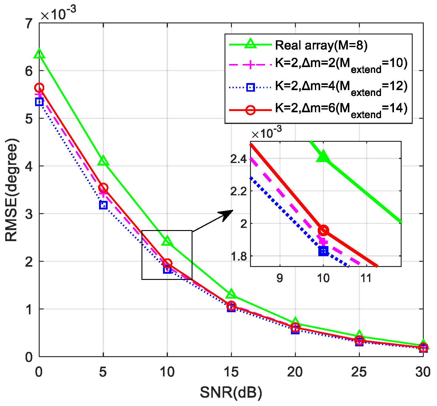
To evaluate the DOA estimation accuracy based on the proposed RD-domain virtual aperture extension, we take $\mathrm{C}=500$ and present the RMSE result in Figure 14.

Figure 14. Single target RMSE results based on the CBF method with different $K$.

In Figure 14, the green dotted line represents the RMSE result based on the CBF method of the real array and the other lines represent the RMSE results based on the CBF method of the extended array.

It shows that the RMSE of the proposed method is lower than that of the real array, indicating that the proposed method can effectively improve the DOA estimation accuracy. Moreover, when $\mathsf{\Delta }\mathrm{m}$ is constant, as $\mathrm{K}$ increases, ${\mathrm{M}}_{\mathrm{extend}}$ increases, and RMSE decreases, resulting in a higher DOA estimation accuracy. Therefore, by increasing $\mathrm{K}$ (i.e., the virtual aperture processing time $\mathrm{KT}$), the DOA estimation performance for a single target can be improved effectively.

Secondly, we simulate the impact of $\mathsf{\Delta }m$ on the proposed virtual aperture extension method by setting the parameters as follows: $\mathsf{\Delta }m\in \{2,4,6\}$, $K=2$.

To evaluate the DOA resolution ability based on the proposed method, we present the DOA estimation results of the CBF method with different $\mathsf{\Delta }m$ in Figure 15.

Figure 15. Single target DOA estimation results based on the CBF method with different $\mathsf{\Delta }m$.

It can be seen that the spatial spectrum distribution of the extended array is more concentrated than that of the real array, which means that the proposed method for a single target can effectively extend the array aperture and enhance the target resolution ability of the DOA estimation method. Figure 15 shows that when $K$ remains constant, the larger the $\mathsf{\Delta }m$, the larger the $M_{\mathrm{extend}}$, the more concentrated the spatial spectrum distribution is, thereby resulting in a better target resolution ability.

To evaluate the DOA estimation accuracy based on the proposed RD-domain virtual aperture extension, we take $C=500$ and present the RMSE result in Figure 16.

Figure 16. Single target RMSE results based on the CBF method with different $\mathsf{\Delta }m$.

It shows that the RMSE result of the extended array is lower than that of the real array, indicating that the proposed method can effectively improve the DOA estimation accuracy. Moreover, when $K$ is constant, as $\mathsf{\Delta }m$ increases from 2 to 4, $M_{\mathrm{extend}}$ increases, and RMSE decreases, resulting in a higher DOA estimation accuracy. However, when $\mathsf{\Delta }m=6$, although $M_{\mathrm{extend}}$ increases, according to the analysis in Section 3.4, the number of element pairs that can be used to estimate $\overline{{\mathsf{\Delta }\phi }_m}$ decreases to $\left(M-\mathsf{\Delta }m\right)=2$, which makes the calculated virtual element’s data more susceptible to noise and results in a decrease in RMSE.

Thirdly, we verified that the proposed method for a single target in Section 3.4 is suitable for both overlapping and non-overlapping array motion manners and is less affected by the motion manner. We take $\mathsf{\Delta }\mathrm{m}=2$, $\mathrm{K}\in \{4,8\}$, and adjust the ship speed ${\mathrm{v}}_{\mathrm{ship}}$ to achieve the ship’s non-overlapping motion. The RMSE result with $\mathrm{C}=500$ is shown in Figure 17.

Figure 17. Single target RMSE results based on the CBF method with different $v_{\mathrm{ship}}$.

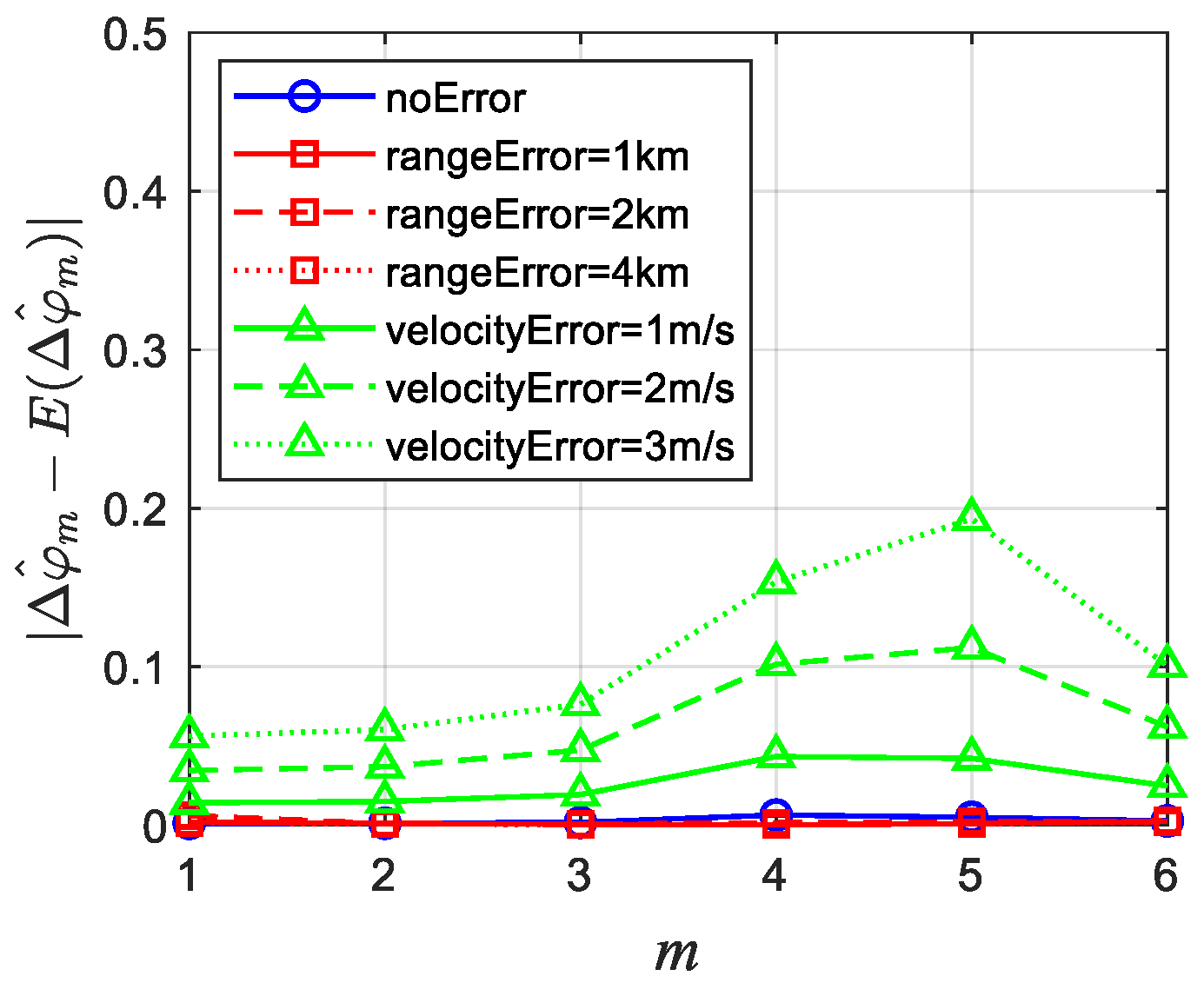
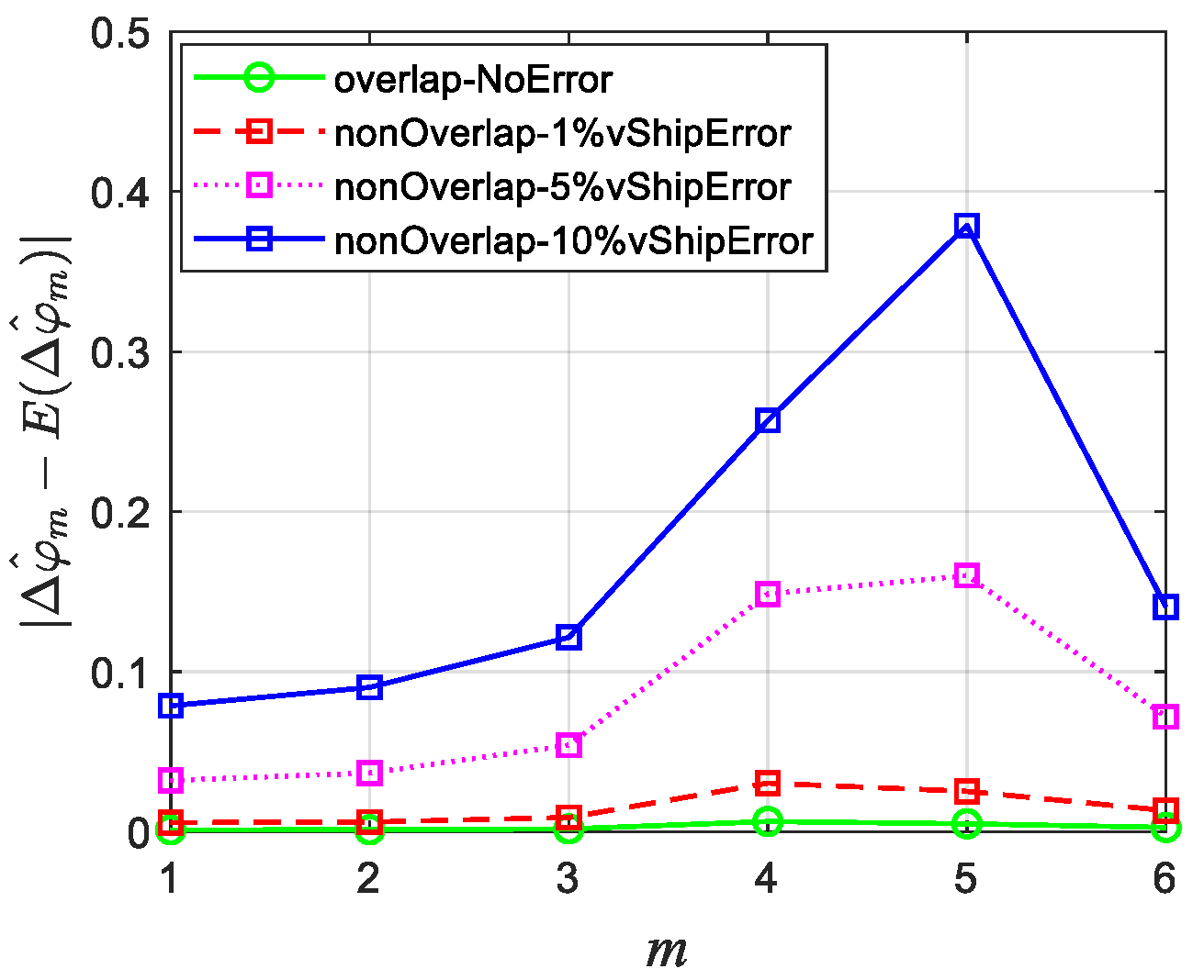
In Figure 17, red lines represent the RMSE results based on the CBF method of the extended array when $\mathrm{K}=4$ and $\mathsf{\Delta }\mathrm{m}=2$ and the blue lines represent the RMSE results based on CBF method of the extended array when $\mathrm{K}=8$ and $\mathsf{\Delta }\mathrm{m}=2$. The solid lines indicate that ${\mathrm{v}}_{\mathrm{ship}}\mathrm{T}=\mathrm{d}$ (i.e., the ship moves in an overlapping manner), the dashed and dotted lines, respectively, indicate that ${\mathrm{v}}_{\mathrm{ship}}\mathrm{T}=0.8 \mathrm{d}$ and ${\mathrm{v}}_{\mathrm{ship}}\mathrm{T}=1.6 \mathrm{d}$ (i.e., the ship moves in a non-overlapping manner), respectively.

It shows that when $\mathsf{\Delta }\mathrm{m}$ and $\mathrm{K}$ are constant (i.e., ${\mathrm{M}}_{\mathrm{extend}}$ is constant), RMSE almost only changes with SNR instead of ${\mathrm{v}}_{\mathrm{ship}}$, which implies that the array of non-overlapping motion has almost no impact on the DOA estimation accuracy. That is, the proposed method for a single target is suitable for both overlapping and non-overlapping array motion manners.

5.2. Simulation of the Proposed Method for Multiple Targets

For multiple targets, according to the analysis in Section 3.5, the number of extended array elements is $M_{\mathrm{extend}}=M+2(K-1)$, which means that $\mathsf{\Delta }m$ is fixed at 2 and the size of the extended aperture is only affected by $K$. By setting the parameters of the two targets $\left(R_i, v_{\mathrm{target}i}, {\theta }_i\right)=\left(51, 100, 20\right)$ and $(51, 100, 30)$, we simulate the impact of $K$ on the proposed virtual aperture extension method.

To evaluate the DOA resolution ability based on the proposed method, we set $K\in \{4,12\}$ and present the DOA estimation results of the CBF method in Figure 18.

Figure 18. Two targets of DOA estimation results based on the CBF method with different $K$.

In Figure 18, the green solid line represents the DOA estimation result based on the CBF method of the real array, the black dashed line represents the target real azimuth, and the other lines represents the DOA estimation results based on the CBF method of the extended array.

It can be seen that when $\mathsf{\Delta }\mathrm{m}$ is constant, as $\mathrm{K}$ increases from 4 to 12, ${\mathrm{M}}_{\mathrm{extend}}$ increases, the spatial spectrum of the two targets can be distinguished more easily, and the two targets’ spectral peaks are closer to the true azimuth. Therefore, the proposed method for multiple targets can effectively extend the array aperture and enhance the target resolution ability of the DOA estimation. Additionally, the larger the $\mathrm{K}$, the better the target resolution ability is.

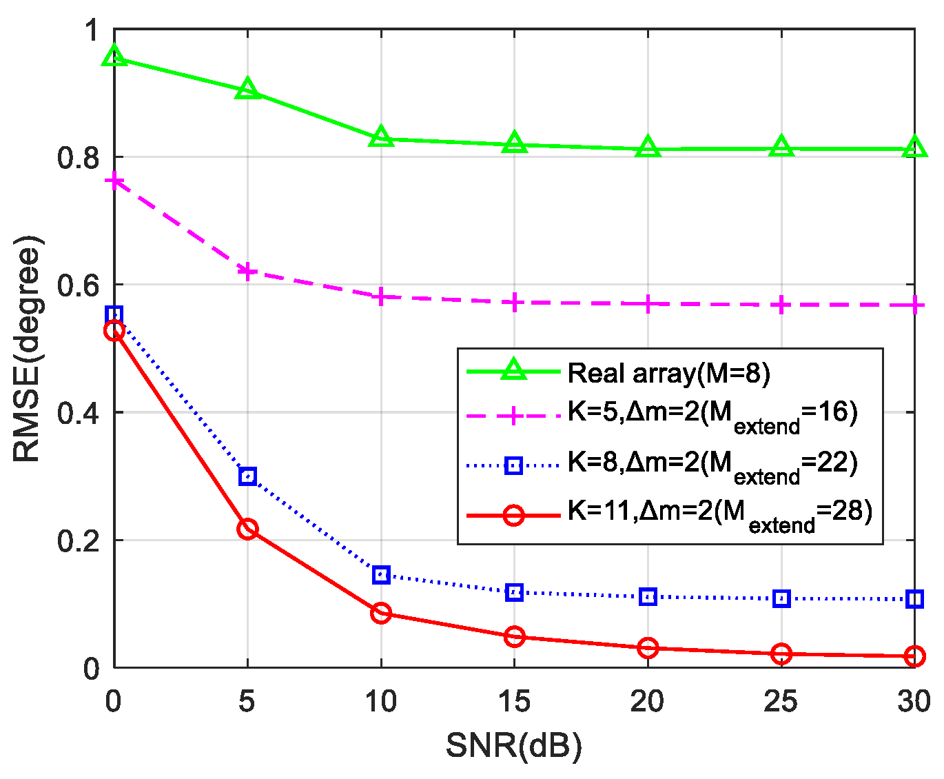
To evaluate the DOA estimation accuracy based on the proposed RD-domain virtual aperture extension, we set $K\in \{5,8,11\}$, $C=500,$ and present the RMSE result in Figure 19.

Figure 19. Two target RMSE results based on the CBF method with different $K$.

In Figure 19, the green dotted line represents the RMSE result based on the CBF method of the real array, and the other lines represent for the RMSE results based on CBF method of the extended array.

It shows that the RMSE result of the extended array is lower than that of the real array, indicating that the proposed method can effectively improve the DOA estimation accuracy. Moreover, when $K$ increases, $M_{\mathrm{extend}}$ increases, and RMSE decreases, resulting in a higher DOA estimation accuracy. Therefore, by increasing $K$, the DOA estimation performance for multiple targets can be improved effectively.

In general, as the ship moves and the virtual aperture processing time (i.e., K) increases, more virtual elements’ data can be estimated through the proposed method. Consequently, the aperture size of the extended array expands, leading to an improvement in the array’s DOA estimation performance.

6. Experimental Results and Discussion

In this section, we use experimental data to further verify the proposed RD-domain virtual aperture extension method. Due to the limitations of the current experimental conditions, we do not yet have real target echoes that meet the required conditions to validate the proposed method. Therefore, we add simulated target echoes to the experimental data to validate the proposed method.

The parameter settings are as follows: the working frequency of the radar system is about 4.7 MHz, the array is configured as an 8-element uniform linear array with an element spacing of 15 m, and the ship speed for the simulated target signals is about 7.5 m/s. Under the following two conditions, we add simulated target signals to the experimental data from various time segments.

For case 1, we add simulated targets with significant differences in range or velocity parameters from clutter to the experimental data. The RD spectrum of the array element 1 in time segment 1 is shown in Figure 20.

Figure 20. RD spectrum of the array element 1 for case 1.

Here, the horizontal axis X in Figure 20 represents the Doppler cells, while the vertical axis Y represents the range cells. The power of each RD cell is depicted using different colors according to its magnitude. We set three simulated targets in two RD cells. In a range-Doppler cell (45, 135), we set a single target with an azimuth angle of 30 degrees. In a range-Doppler cell (851, 340), we set two targets with identical range and velocity parameters, and an azimuth angles of 20 degrees and 30 degrees, respectively.

Then, using the CBF method, we perform DOA estimation on the RD cells where the simulated targets are located, as shown in Figure 21.

Figure 21. DOA estimation results based on the CBF method. (a) Single target in an RD cell (45, 135). (b) Two targets in an RD cell (851, 340).

Here, the red solid line represents the CBF method DOA estimation result of the real array, the blue and green dashed lines represent the results of extended array, and the black dotted lines represent the targets’ real azimuth. In Figure 21a, it can be seen that the spatial spectrum distribution of the extended array is more concentrated than that of the real array, which means the proposed method for a single target is effective. Figure 21b shows that the two targets’ spatial spectrum of the extended array can be distinguished more easily than that of the real array, which means the proposed method for multiple targets is effective.

Table 2 presents the numerical results of DOA estimation error for case 1; it can be seen that the DOA estimation error of the extended array is smaller than that of the real array, representing a higher DOA estimation accuracy. Moreover, as the number of virtual array elements increases, the DOA estimation accuracy improves accordingly.

Table 2. Numerical results of the DOA estimation error for case 1.

		Real Array	Extended Array Based on Proposed Method
Number of Array Elements		M = 8	$M_{\mathrm{extend}}$= 12 $(K=3, \mathsf{\Delta }m$ = 2)	$M_{\mathrm{extend}}$ = 14 $(K=4, \mathsf{\Delta }m$ = 2)	$M_{\mathrm{extend}}$ = 16 $(K=5, \mathsf{\Delta }m$ = 2)	$M_{\mathrm{extend}}$ = 20 $(K=5, \mathsf{\Delta }m$ = 3)
DOA Estimation Error (°)	Single Target	0.0265	0.0189	0.0126	0.0083	0.0044
	Two Targets	2.2643	1.8544	1.1632	0.6752	-

For case 2, we add simulated targets with range and velocity parameters close to the clutter into the experimental data. The RD spectrum of the array element 1 in time segment 1 is shown in Figure 22.

Figure 22. RD spectrum of the array element 1 for case 2.

In this case, we also set three simulated targets in two RD cells. In a range-Doppler cell (45, 950), we set a single target with an azimuth angle of 30 degrees. In a range-Doppler cell (851, 120), we set two targets with identical range and velocity parameters, and azimuth angles of 20 degrees and 30 degrees, respectively.

Then, using the CBF method, we perform DOA estimation on the RD cells where the simulated targets are located, as shown in Figure 23. It can be seen that the targets’ spatial spectrum of the extended array is more concentrated and easier to distinguish than that of the real array, which means the proposed method is effective. However, due to the effect of clutter, the target data extracted from the RD unit may be inaccurate, resulting in a decrease in DOA estimation performance in case 2 compared to case 1. In this case, clutter suppression may improve the performance of DOA estimation, which may be analyzed in our future research.

Figure 23. DOA estimation results based on CBF method. (a) Single target in RD cell (45, 950). (b) Two targets in RD cell (851, 120).

Table 3 presents the numerical results of DOA estimation error for case 2. Compared to case 1, the DOA estimation accuracy in case 2 may decrease due to the effect of clutter. However, it can be seen that the DOA estimation performance of the extended array remains superior to that of the real array and continues to improve as the number of virtual array elements increases.

Table 3. Numerical results of DOA estimation error for case 2.

		Real Array	Extended Array Based on Proposed Method
Number of Array Elements		M = 8	$M_{\mathrm{extend}}$ = 12 $(K=3, \mathsf{\Delta }m$ = 2)	$M_{\mathrm{extend}}$ = 14 $(K=4, \mathsf{\Delta }m$ = 2)	$M_{\mathrm{extend}}$ = 16 $(K=5, \mathsf{\Delta }m$ = 2)	$M_{\mathrm{extend}}$ = 20 $(K=5, \mathsf{\Delta }m$ = 3)
DOA Estimation Error (°)	Single Target	4.2156	2.6748	1.6456	0.7798	0.1321
	Two Targets	5.9785	3.4785	1.7147	0.9720	-

7. Conclusions

This paper proposes an RD-domain virtual aperture extension method to address the problem of small aperture and poor DOA estimation performance for shipborne HFSWR. Through this method, we effectively extend the array aperture and improve the DOA estimation performance of shipborne HFSWR. The summary of this paper is as follows. Firstly, we establish a continuous motion model based on the validity of far-field assumption and provide a novel flowchart for the proposed method. Secondly, based on the signal time–domain segmentation model, we derive the proposed RD-domain virtual aperture extension method for a single target and multiple targets. Thirdly, we analyze the performance of the proposed method through simulations. Finally, we verify the proposed method through simulation experiments and experimental data.

In general, this work has the following implications. (1) By extending the traditional time–domain virtual aperture extension method to the RD domain, targets in strong clutter backgrounds can be distinguished, and therefore, the target resolution capability can be improved through virtual aperture extension. (2) Based on the RD-domain processing, targets with different ranges or velocities can be separated, thereby allowing the application of the virtual aperture extension method to them. (3) In the case of a single target, it does not require the array to move in an overlapping manner.