Article

A New Multimodal Map Building Method Using Multiple Object Tracking and Gaussian Process Regression

Division of Electronic Engineering, Jeonbuk National University, Jeonju 54896, Republic of Korea
*
Author to whom correspondence should be addressed.
Remote Sens. 2024, 16(14), 2622; https://doi.org/10.3390/rs16142622
Submission received: 5 June 2024 / Revised: 12 July 2024 / Accepted: 16 July 2024 / Published: 18 July 2024
(This article belongs to the Special Issue Deep Learning for Remote Sensing and Geodata)

Abstract

:
Recent advancements in simultaneous localization and mapping (SLAM) have significantly improved the handling of dynamic objects. Traditionally, SLAM systems mitigate the impact of dynamic objects by extracting, matching, and tracking features. However, in real-world scenarios, dynamic object information critically influences decision-making processes in autonomous navigation. To address this, we present a novel approach for incorporating dynamic object information into map representations, providing valuable insights for understanding movement context and estimating collision risks. Our method leverages on-site mobile robots and multiple object tracking (MOT) to gather activation levels. We propose a multimodal map framework that integrates occupancy maps obtained through SLAM with Gaussian process (GP) modeling to quantify the activation levels of dynamic objects. The Gaussian process method utilizes a map-based grid cell algorithm that distinguishes regions with varying activation levels while providing confidence measures. To validate the practical effectiveness of our approach, we also propose a method to calculate additional costs from the generated maps for global path planning. This results in path generation through less congested areas, enabling more informative navigation compared to traditional methods. Our approach is validated using a diverse dataset collected from crowded environments such as a library and public square and is demonstrated to be intuitive and to accurately provide activation levels.

Graphical Abstract

1. Introduction

In the field of autonomous driving, maps are a crucial element for mobility platforms to perceive their surroundings and plan their paths. Maps provide information about the environment to the vehicles or robots and can be constructed through simultaneous localization and mapping (SLAM) technology [1,2,3,4]. SLAM performs localization and mapping tasks for intelligent mobile platform navigation, such as for autonomous vehicles or robots. It is a key part of the robotics field and requires accurate and efficient representation of the environment and current location estimation for navigating in unknown environments. Accurate and reliable location recognition performance and proper map building are the core goals of SLAM technology.
The form of the map varies depending on how the environment is represented. A commonly used type of map is the geometric map. Geometric maps represent the environment with geometric information such as points, lines, planes, grids, etc. They have the advantage of intuitively representing the real world, as they contain the appearance of the environment. Existing studies on creating geometric maps tend to remove dynamic objects [5,6,7,8]. This is for two main reasons. First, dynamic objects are considered temporary features that exist only at the time of map creation and are deemed unnecessary for long-term map use. Second, the rapid movement of dynamic objects is considered noise in the map creation process, and their removal is aimed at improving the accuracy of the map. For these reasons, information about dynamic objects is typically removed during the map-making process and is used in real-time for path planning after the map is created. However, the information from dynamic objects can provide essential insights into understanding their behavior in that particular space. For example, in complex environments such as libraries, department stores, and squares, dynamic objects can help determine which areas are active. This information simultaneously becomes information about inactive areas. Understanding the dynamic characteristics of these objects plays a crucial role in the information-based operation of robots or vehicles and for more efficient path planning.
The main objective of this study is to include the trajectory information of such dynamic objects in the geometric map to provide information about potentially moving objects. For this purpose, our proposed method first performs model-free multiple object tracking (MOT) using LiDAR sensors [9]. Tracking is performed without prior information about moving objects, allowing it to include information about all moving objects. MOT estimates the IDs, positions, and velocities of multiple targets. After capturing the trajectories of all estimated targets, non-dynamic noise such as walls and pillars is filtered out, and Gaussian process regression (GPR) is applied. GPR interpolates the data by reflecting the correlation of each point in the sparse trajectories of targets and effectively models their uncertainty. Finally, the level of target activity, which represents the spatial frequency values of dynamic objects obtained through GPR, is overlaid on the OG map. The occupancy state values of the OG map (free, occupied, or unknown) are combined with the level of target activity to form an expanded multimodal map that provides additional information. This map has been named the target activity (TA) map in our research.
To the best of our knowledge, our proposed method is the first study to include LiDAR-based tracking information of dynamic objects in SLAM-based map construction. The contributions of this paper can be summarized as follows:
  • A robot-based map building framework is proposed that utilizes model-free multiple object tracking (MOT) integrated with dynamic object information along with 2D occupancy maps derived from SLAM.
  • We propose a multimodal map, called the TA map, that represents the level of target activity on the OG map. This map can help with path planning for autonomous navigation.
  • A registration of multiple target trajectories is developed to create a generalized map. Thus, sensor data obtained under various dataset acquisition conditions, such as different times, routes, and starting points, can be integrated into a single multimodal map.
This framework enables effective operation in environments ranging from expansive to intricate, showcasing its adaptability to various environments. It also facilitates the addition and removal of datasets, enabling the creation of a more generalized map.
This paper is organized as follows: Section 2 discusses related research. Section 3 presents the problem statement, outlines the fundamentals of SLAM and MOT, and defines the specific problem this research addresses, along with the basic approach for its resolution. Section 4 proposes a method for creating a multimodal map using MOT and GPR. Section 5 presents the results based on our custom dataset in indoor and outdoor scenarios, including the use of the TA map for path planning. Section 6 addresses the limitations of the proposed method. Finally, Section 7 discusses the expected effects of this research and directions for future research.

2. Related Work

Accurately identifying both dynamic objects and the static environment is necessary for representing environments. Multiple object tracking (MOT) has emerged as a significant research area for determining dynamic objects, while concurrently, research on map creation is essential for understanding the static environment. Although traditional map building methods use continuous sensor data to construct maps using static elements, recent studies have been actively focusing on creating maps that include not only static structures but also a variety of other information. In this process, the use of the Gaussian process in map building plays a crucial role in reducing data uncertainty and enhancing the accuracy of predictions.

2.1. Multiple Object Tracking (MOT)

MOT is one of the methods for real-time understanding of the surrounding environment. It involves the detection [10,11,12] and tracking of multiple objects through LiDAR or cameras. Choi et al. [9] use LiDAR to recognize dynamic objects through normal distribution transform (NDT) inference. This research has become the base of our MOT framework. There are MOT studies using cameras, such as [13,14,15]. Generally, MOT is linked to real-time local path planning [16,17,18,19]. In our research, this information has been represented on the map. Thus, robots can perform global path planning based on information about dynamic objects while utilizing geometric information.

2.2. Maps Containing Dynamic Object Information

Research on mapping the motion information of dynamic objects includes the following: Rudenko et al. [20] created an occupancy map that includes areas where human motion is expected using only a semantic map and CNN. Almonfrey et al. [21] used the tracking results of humans with four cameras to create a cumulative occupancy map showing the most visited places. Kuncer et al. [22] presented a new approach to model movement patterns using partial observations of human motion direction and speed. Wang et al. [23] proposed a method that segments the environment into structured areas and semantically classifies [24] the motion information of dynamic objects in each area. Vintr et al. [25] clustered the spatio–temporal vector space to represent the movements of dynamic objects as periodic temporal patterns. Nevertheless, these studies create maps of various forms rather than geometric maps, making them not easy for robots to use directly. Additionally, there is a limitation in that the sensors used to collect the motion information of dynamic objects are fixed.

2.3. Map Building with Gaussian Process

The Gaussian process (GP) [26,27,28] is widely used in complex data analysis and map making due to its effective performance in data estimation and prediction. It provides strong results, especially in data environments with uncertainty. Guo et al. [29] combined a GP with an object detection and tracking framework to enable path planning. In this process, the GP was utilized to create a risk map based on the framework’s results, which was then applied in the path planning process. West et al. [30] used GP to represent the detection level of radioactive elements on an OG map. In human motion modeling works, O’Callaghan et al. [31] proposed a method of creating a navigation map for robots using GPR, focusing on analyzing movement patterns in terms of the deviation angles of human trajectories. Stuede et al. [32] presented a novel method using GPR for spatio–temporal modeling of human activity based on human motion observation in specific environments. However, the tracking dataset used in this paper was limited to the single-fixed-LiDAR-based Office dataset [33] and the fixed 3D range sensors used in the ATC dataset [34]. When using fixed sensors, sufficient data can be acquired for a specific space, but adaptability to various environments is lacking. In this case, using a single sensor only enables the collection of information within a limited range. On the other hand, using multiple sensors leads to higher costs and complexity.
Our method easily collects tracking data for complex and large-scale environments using a robot-based framework. Also, the proposed method creates a new map that contains not only static structural information from SLAM but also dynamic object information from MOT. To incorporate both sets of information, we employ the GPR and developed a new TA map building algorithm. Furthermore, a registration method for multiple target trajectories is developed to include data acquired at multiple time points into a single map.

3. Problem Statement

In this section, the preliminary fundamentals, including a brief introduction to conventional SLAM and MOT, are presented. Furthermore, this part defines the problem it aims to solve and explains the basic idea for solving it.

3.1. Problem Definition

Assume that a sensor is navigating in an unknown environment and captures 3D pointcloud inputs P t at time step t. Using sensor information, the goal of the SLAM algorithm is to estimate the 6-DOF sensor pose x s e n s o r , t and registered pointcloud m t for each time step t.
On the other hand, MOT estimates the states x t a r g e t , t = { x t 1 , , x t N t } of multiple targets through sensor input, where N t is the number of target objects at time t. As a result of MOT, the i-th target at time t is represented as x t i = [ i , p x , t i , p y , t i , v x , t i , v y , t i ] T . Each element indicates a target ID, two-dimensional position, and velocity, respectively. A previous work that uses NDT for tracking [9] estimates the displacements of dynamic objects from t 1 to t using a mixture of normal distribution matching. Thus, each target is represented as a mean and covariance of a mixture of multivariate normal distributions.
At each time step, we can obtain the state vector for multiple targets and the state of ego-motion X t = { x s e n s o r , t , x t a r g e t , t } through MOT and SLAM concurrently. Additionally, the trajectories of the sensor and targets for all steps are represented as follows:
X = { X t } t = 1 T
Using this information, the goal is to build a multimodal map.
M = arg max p ( M | X )
Meanwhile, our multimodal map M takes the following form:
M = [ m 1 , , m N g ] m i = [ i , o i ] T , i = 1 , , N g
where N g denotes the number of grid cells, and i , o i indicate the level of target activity and the occupancy value of each grid cell, respectively.

3.2. Basic Idea

Mainly, SLAM struggles with the capability to distinguish between static and dynamic objects, resulting in the inclusion of traces from moving objects within the map, as illustrated in Figure 1. This deficiency can become a source of unexpected errors in path planning for autonomous driving.
To address this issue, this paper employs model-free MOT [9] to gather information about moving objects and integrate it into a single map. This approach can aid with path planning by additionally generating information about spaces where traces of moving objects frequently appear during SLAM.
First, the trajectories of multiple targets obtained from MOT are converted into global coordinates. Subsequently, by using the proposed filtering algorithm, only the robust targets will be retained. Then, we calculate the number of moving targets that exist in a specific grid cell, which is a discontinuous space.
To incorporate the track information of discontinuous objects found during robot navigation into continuous areas, regression is needed. This regression estimates the track information at arbitrary positions based on the obtained track data. We represent information about moving objects on the map using GPR. It can predict the continuous values at test map positions. Here, the continuous value can be considered to be the degree of moving targets. In other words, a level of target activity is represented by a function f ( x ) as follows:
f ( x ) GP ( μ ( x ) , k ( x , x ) )
This equation represents the function f ( x ) as a GP with a mean function μ ( x ) and a covariance function k ( x , x ) , where the mean is a constant and the covariance is given by the radial basis function (RBF) kernel. Detailed information is provided in Section 4.3.

4. Proposed Method

4.1. Overview

As discussed in Section 1 and Section 2, existing research on creating geometric maps for robots tends to remove information about dynamic objects, resulting in the loss of essential dynamic information. Conversely, studies that include information about dynamic objects create various forms of maps, but these are not suitable for direct use by robots, and data collection from fixed sensors limits scalability and flexibility. To address these issues, our study proposes a novel ego-robot-based framework that uses SLAM to generate geometric maps and integrates dynamic object information from MOT.
Our proposed method utilizes a LiDAR sensor mounted on a mobile robot. As can be seen in Figure 2, the MOT and SLAM [4] modules operate simultaneously. This framework allows us to generate multiple target trajectories in a global coordinate system. Since these trajectories can include trajectories from not only dynamic objects but also non-dynamic objects, we use a filtering process to remove outliers and generate refined trajectories that only consist of dynamic targets. Subsequently, we divide the entire map into specific-sized grid cells. At each point of the dynamic target trajectory x t i , we calculate the level of target activity, which is defined as the number of targets present within each grid cell. Even for areas where the target does not appear, the activity level is estimated through GRP. This estimated level of target activity is integrated with an OG map to effectively represent the spatial distribution of dynamic targets within the environment as a TA map.
When the robot is running at a new point in time, the generated maps and trajectories become individual datasets based on the time and initial location of the robot’s sensor data collection. Therefore, we can optionally apply a registration method that estimates the correlation between maps and integrates the trajectories of each dataset onto a single reference map.

4.2. Multiple Target Trajectories and Filtering

The trajectories for multiple targets are based on the LiDAR coordinates and are only plotted within a predefined tracking range of ± r ( m ) . Therefore, they need to be transformed into world coordinates.
Since the MOT algorithm may generate wrong results, outliers that are predicted to be dynamic objects are sometimes created for static structures such as building columns and trees. This section introduces a method to filter out such outliers.

4.2.1. LiDAR Coordinates to World Coordinates

The trajectories for multiple targets are recognized within a radius of ± r ( m ) based on LiDAR coordinates, so they should be converted to world coordinates using the robot’s pose.
x ^ t a r g e t , t = x t a r g e t , t x s e n s o r , t
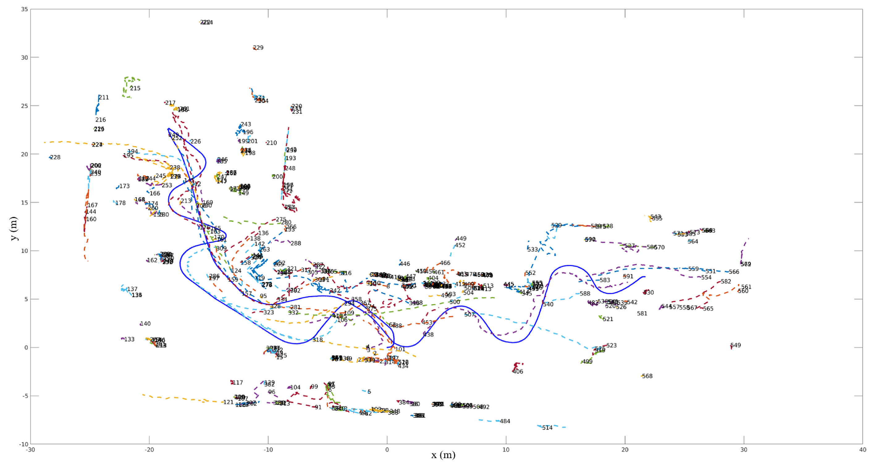
where x s e n s o r , t represents the robot’s pose obtained from LiDAR SLAM. Also, the operator ⊕ denotes the pose composition operator [35]. The transformed trajectory of the targets and the robot’s trajectory are depicted in Figure 3, where the targets are represented with dotted lines and the robot is shown with a solid blue line. The numbers attached to each dotted line represent the ID of the target. As can be seen in Figure 3, the total number of targets is quite large, and unnecessary dummy targets remain.

4.2.2. Dummy Target Filtering

As seen in Figure 3, the multiple target trajectories include noise originating from pillars or walls. To filter out these non-dynamic targets, Algorithm 1 is executed.
Algorithm 1: Dummy target filtering
  1:
Initialize: total target number N, Filtered_Array = [ ]
  2:
for  i = 1 to N do
  3:
     S = s i z e o f ( x t i )
  4:
     ( p x , t 0 i , p y , t 0 i ) start position of i-th target in world coordinate
  5:
     ( p x , t S i , p y , t S i ) end position of i-th target in world coordinate
  6:
     d i s t = ( p x , t S i p x , t 0 i ) 2 + ( p y , t S i p y , t 0 i ) 2
  7:
     v x , a v g i , v y , a v g i = 1 S j = 0 S v x , t j i , 1 S j = 0 S v y , t j i
  8:
     v = v x , a v g i 2 + v y , a v g i 2
  9:
    if  ( S α ) ( d i s t β ) ( v γ )  then
10:
        Filtered_Array.append( ( i , { ( p x , t j i , p y , t j i ) } j = 1 S ) )
11:
    end if
12:
end for
    Algorithm 1 is based on the following characteristics of non-dynamic targets:
  • Minimal pose variation: non-dynamic objects exhibit minimal changes in their poses over time.
  • Low velocity: they have a low or negligible velocity since they remain stationary.
  • Compactness: non-dynamic objects tend to have compact spatial distributions, resulting in small-sized vectors.
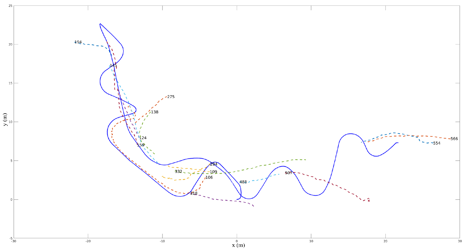
In the dummy target filtering process, for each target, the trajectory size, the Euclidean distance between the first and last pose, and the average speed are calculated (lines 6–8). A target is only retained if it exceeds the heuristically set threshold α , β , γ for each value (line 9). Targets that do not meet this criterion are excluded from the filtering process (line 10). The targets that pass are considered filtered results, and these results can be verified in Figure 4. Such filtering methods effectively remove dummy data, contributing to the accuracy of MOT.

4.3. TA Map Generation with GPR

Since the TA map is represented as m i = [ i , o i ] T , i = 1 , , N g and the level of activity and occupancy terms are independent of each other, i.e., i o i , therefore, the posterior of the SLAM problem can be derived as follows:
p ( x 1 : t , m | z 1 : t , u 1 : t ) = p ( x 1 : t | z 1 : t , u 1 : t ) p ( m | x 1 : t , z 1 : t ) = p ( x 1 : t | z 1 : t , u 1 : t ) p ( m o | x 1 : t , z 1 : t o ) p ( m | x 1 : t , z 1 : t ) p ( x 1 : t | z 1 : t , u 1 : t ) i = 1 N p ( m o , i | x 1 : t , z 1 : t o ) p ( m , i | x 1 : t , z 1 : t )
where m = i i = 1 , , N g , and m o = o i i = 1 , , N g .
To estimate the second term of the posterior above, we estimate the occupancy value of the corresponding cell given S points of dataset observations. For the estimation of a single cell o i , the maximum likelihood estimate (MLE) of the mean and variance are given by
μ o , i = 1 S n = 1 S p z n σ o , i 2 = 1 S n = 1 S p z n μ n p z n μ n T
where p z n is the probability of end point location of the scan data. Applying Equation (7) to each grid cell, occupancy map m o is represented by μ o = μ o , 1 μ o , 2 μ o , N g T . This matrix μ o can be considered as the mean of the multivariate Gaussian distribution. Under the assumption that every cell is independent of the others, the corresponding covariance matrix is given by
Σ o = σ o , 1 2 0 0 0 0 0 0 σ o , N g 2
Unlike the occupancy map, for the level of the target activity map m , after the filtering process in Section 4.2, we define the training dataset for GPR in the form of D = { ( p i , i ) } i = 1 N . Here, the input p i represents the world coordinate base position information of the filtered i-th target and is defined as follows: p i = { ( p x , t j i , p y , t j i ) } j = 0 S , where p i F . Here, F represents the coordinate pairs obtained from the filtered array. F = { p ^ x , p ^ y | ( p ^ x , p ^ y ) F i t e r e d a r r a y } . The set that includes ( p ^ x , p ^ y ) is the result of the coordinate transformation through Equation (5).
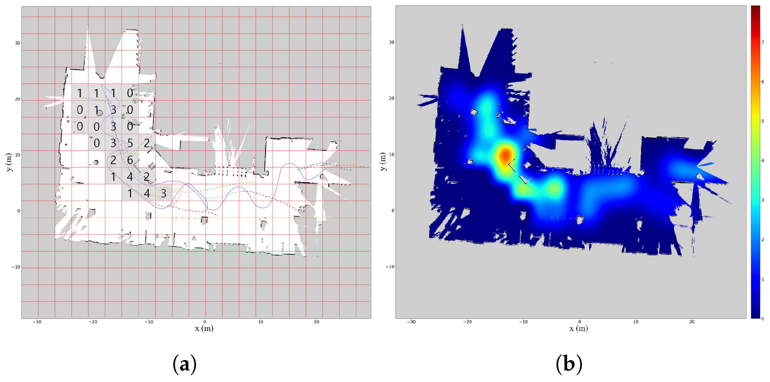
The level of target activity at this position is denoted as i = { t j i } j = 0 S , which can be obtained through Algorithm 2. This represents the total number of targets observed within a specific grid cell, which becomes an important indicator for understanding the distribution and density of dynamic objects on the map. The OG map is divided by a predefined grid size k to set up a dimension composed of grid cells (lines 3–6). Based on this, we traverse the entire grid cell and calculate for each cell (lines 7–13). Then, we find the grid for all positions of the filtered dynamic target and assign to the position (lines 14–18). The results of Algorithm 2 are visualized in Figure 5a.
Algorithm 2: Grid cell algorithm
  1:
Input: Filtered_Array from Algorithm 1, 2D occupancy grid map
  2:
Output: Level of target activity
  3:
Parameter: grid size k
  4:
g r i d _ x # of x grids
  5:
g r i d _ y # of y grids
  6:
g r i d _ a r r a y array [ g r i d _ x ] [ g r i d _ y ]
  7:
for  r o w = 1 to g r i d _ x  do
  8:
    for  c o l = 1 to g r i d _ y  do
  9:
         g r i d _ c e l l [ r o w , c o l ] Region of occupancy grid map divided by grid size k
10:
         Total number of dynamic target trajectories in g r i d _ c e l l [ r o w , c o l ]
11:
         g r i d _ a r r a y [ r o w , c o l ] =
12:
    end for
13:
end for
14:
for i = 1 to size ( F i l t e r e d _ A r r a y )  do
15:
     r o w , c o l Index of Filtered_Array [ i ]
16:
     = Value of g r i d _ a r r a y [ r o w , c o l ]
17:
     F i l t e r e d _ A r r a y [ i ] . a p p e n d ( )
18:
end for
Gaussian process regression generalizes multivariate Gaussian distributions to an infinite-dimensional space, serving as a non-parametric method to model the distribution of functions based on observational data [28]. GPR is defined by a mean function m ( x ) and a covariance function k ( p , p ) . The mean function is often assumed to be zero across the entire input space (i.e., m ( x ) = 0), and the covariance function is used to characterize the relationship between inputs.
f ( x ) GP ( 0 , k ( p , p ) )
In our research, the covariance function utilized is the widely used radial basis function (RBF), which includes a hyperparameter σ 2 , l to model points in space.
k ( p , p ) = σ 2 exp ( p p 2 2 l 2 )
Based on the dataset D = { ( p i , i ) } i = 1 N , GPR was employed to carry out a posterior process for the map point p * . By calculating the mean of the posterior distribution and mapping it, we can get the level of target activity across continuous regions on the OG map. The TA map is created by simultaneously representing and o. For the convenience of visualization, the level of target activity is represented in color only for grid cells where the occupancy value indicates free space. Areas of high activity level are denoted in red, while regions with lower levels of activity are indicated in blue, as illustrated in Figure 5b.
GPR is effective for modeling sparse dynamic object trajectories in multiple dimensions, and it is used to estimate the locations and activity levels of targets as arbitrary continuous functions in Euclidean space. This contributes to building the TA map.

4.4. Registration of Multiple Target Trajectories

Understanding the overall activation characteristics of dynamic objects using only a single dataset is a challenging task. As a consequence, the robot may not perfectly build a map covering all areas of the environment, or the dynamic objects may exhibit different movements at various times. This results in inconsistent Gaussian process outcomes from the collected dataset. Moreover, the outcomes of maps obtained from the same environment can differ depending on the robot’s initial position or orientation. To overcome these issues, a new algorithm is needed that effectively aligns and integrates map and dynamic object trajectory information collected from various directions, positions, and times to generalize the movement of dynamic objects.
First, features are extracted from each OG map and converted from pixel-based to actual metric units. This conversion involves transforming each feature point u , v to real-world coordinates x W , y W , defined by Equation (11).
x W = u · Δ r e s + x o r i g i n y W = ( H m a p v 1 ) · Δ r e s + y o r i g i n
Here, Δ r e s represents the resolution of the OG map, x o r i g i n , y o r i g i n is the origin of the map, and H m a p is the height of the map image. This conversion includes adjustments for the inverted y-axis relationship of the OG map’s pixel coordinates.
Subsequently, for the registration process, a reference map is chosen, and feature matching is conducted between the reference and the other source maps. We used Umeyama’s method [36] to estimate the transformation between metric-scale feature vectors based on these relationships. As a result, we obtained a rotation matrix R k and translation t k that transform the respective dynamic target trajectories from the source dataset to align with the location on the reference map, as defined in Equation (12). This process is shown in Figure 6.
p i , k = p i , k R k + t k , k { 1 , . . , n } p i , t o t a l = p i , r e f + k = 1 n p i , k
where n is the total number of the source dataset, and p i , k refers to the points of the dynamic target trajectory obtained from the k-th source dataset. Additionally, p i , r e f are points from the reference target trajectory that are used directly without transformation. The p i , t o t a l calculated through Equation (12) are the registered points on the reference map.
Through this transformation process, trajectories collected at different times, locations, and orientations can be registered into one. Subsequently, p i , t o t a l and the reference map are used to perform Algorithm 2 to calculate i , t o t a l , and after normalization, we form the dataset D = { ( p i , t o t a l , i , t o t a l n + 1 ) } i = 1 N t o t a l for regression. Following this, GPR is conducted to effectively represent the movements of dynamic objects in a complex environment on a single TA map.

5. Experiments

Datasets for this study were collected in two common environments: an indoor library and an outdoor square at Jeonbuk National University, South Korea. In the library, data acquisition primarily took place near the entrance, with the robot oriented in various directions to capture diverse data. Conversely, in the outdoor square, data collection involved positioning the robot at different cardinal points around the square, with each position facing towards its respective entrance.
Following the data acquisition in these varied environments, experiments were conducted with the following parameters: σ 2 = 1 and grid size = 3 × 3 m. The value of l in GPR for the TA map was set to 2 for the Library case and 2.5 for the Square case. These parameters were heuristically determined to better represent the TA map. We implemented our method using the MATLAB and Python-based Gaussian process framework, GPy [37]. Given the O ( n 3 ) complexity of the Gaussian process, a downsampling process was employed when dealing with a large number of data points.

5.1. Platform

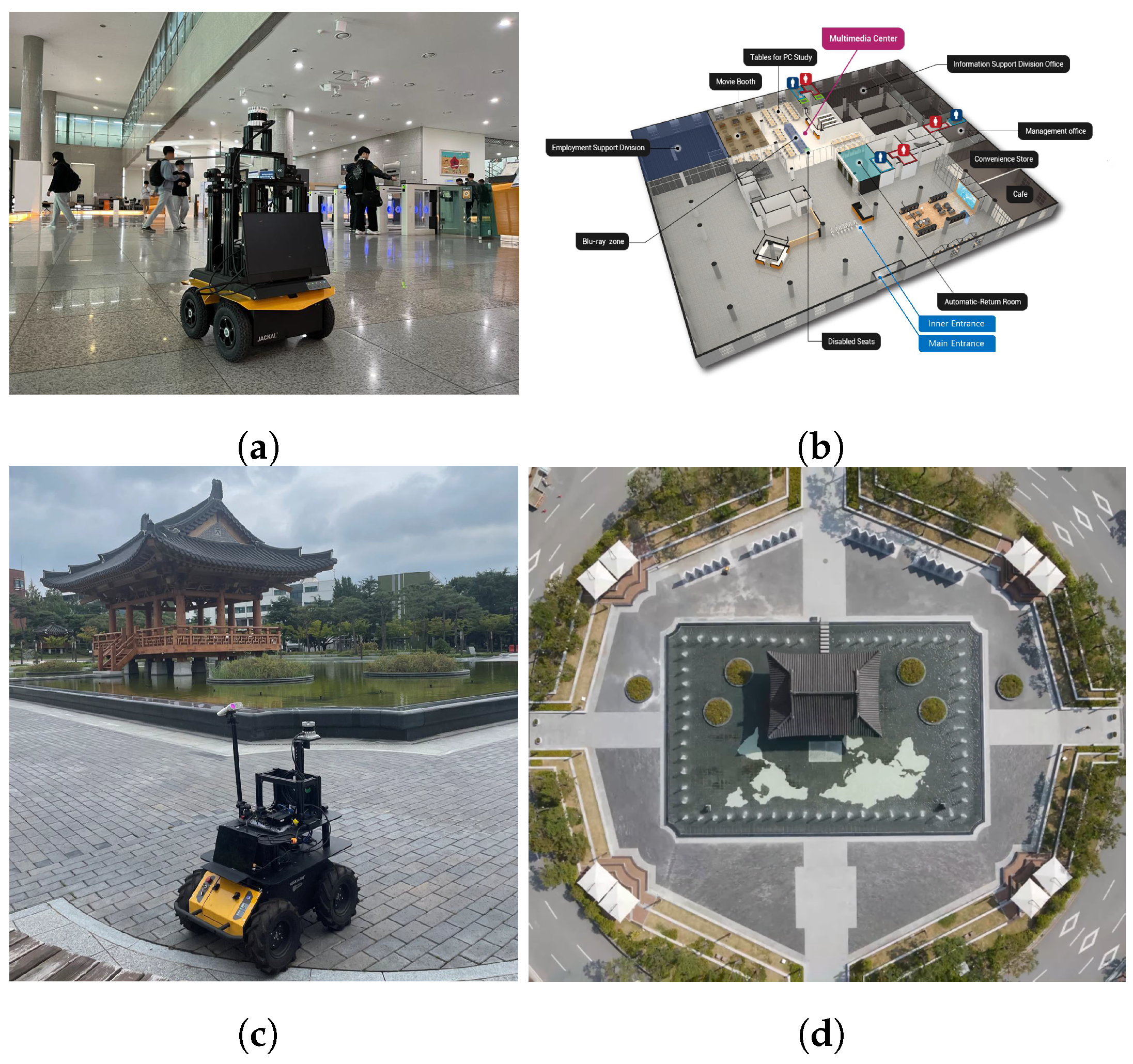
The unmanned ground vehicles (UGVs) used were the Clearpath Jackal and Husky. Figure 7a illustrates the Jackal in the library environment. Figure 7b is a floor guide that offers context for understanding the indoor environment. The Jackal was equipped with an Ouster OS0-32 3D LiDAR. Figure 7c shows the Husky in the outdoor square environment, while Figure 7d shows an aerial view of the area to provide perspective on the outdoor dataset collection. The Husky was utilized with an Ouster OS1-32 3D LiDAR. Within the MOT framework, the detection range for the Jackal was set to ±10 m, which was tailored for the Library dataset. Conversely, the detection range for the Husky was extended to ±20 m to accommodate the larger, open environment of the Square dataset. Table 1 provides detailed information about the Library and Square datasets, including the number of unfiltered and filtered targets, map sizes in pixels and metrics, robot trajectory lengths, and data acquisition times.

5.2. Results for Single Datasets

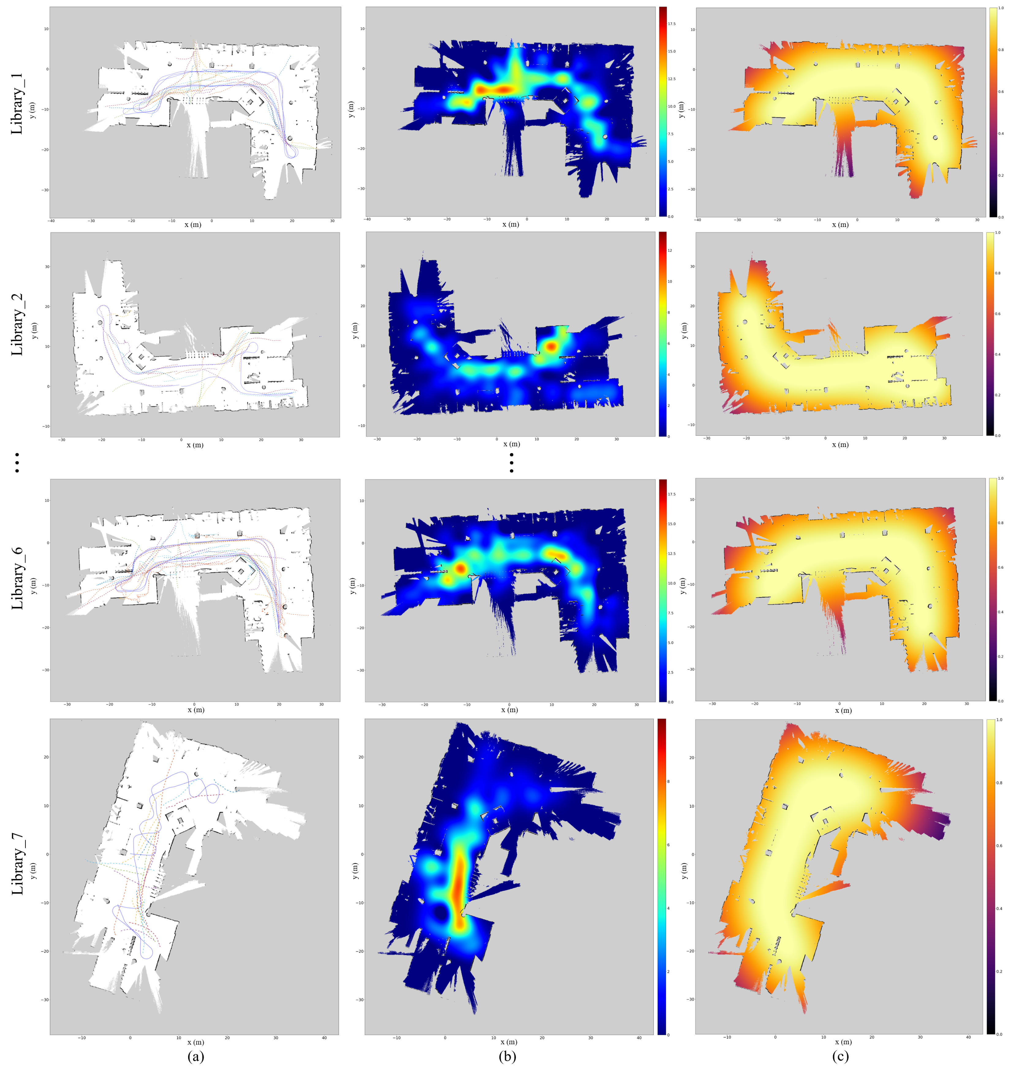
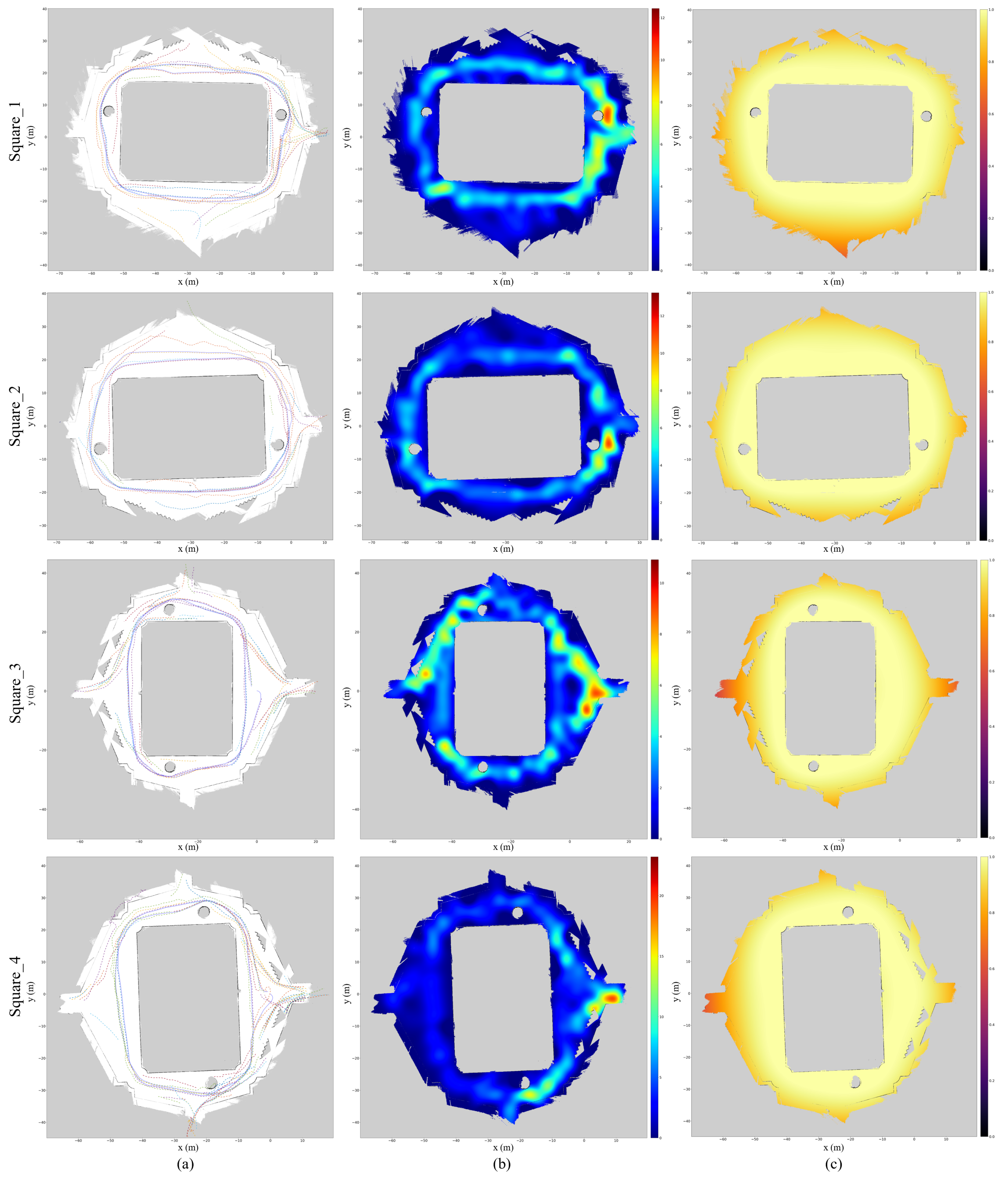
Experiments were conducted with seven Library datasets and four Square datasets. In Figure 8a and Figure 9a, the trajectories of filtered dynamic targets and the robot’s trajectory are overlaid on the OG map obtained through SLAM, allowing observation of how the surrounding targets moved while the robot was acquiring data. For both datasets, Figure 8a and Figure 9a were divided into 3 × 3 m grid cells to calculate the level of target activity. After forming a dataset D = { ( p i , i ) } i = 1 N comprising pairs of dynamic target positions p i and their corresponding levels of target activity i , we created a TA map using GPR, as illustrated in Figure 8b and Figure 9b.
To ensure the reliability of the TA map, a confidence map was created using GPR. This map can be seen in Figure 8c and Figure 9c. The confidence map is crucial for assessing the local-level reliability of target activities on the TA map and distinguishing between areas of low and high reliability. This means that even within the same activity level, the significance of the values can vary depending on their reliability. The confidence map was generated using only the robot’s trajectory, without applying a grid cell algorithm. The GPR kernel used was the RBF kernel, and the lengthscale l was set according to the target tracking range in the MOT framework (10 m and 20 m, respectively).
As evidenced by the analysis in Figure 8 and Figure 9, the TA maps of single datasets vary based on the starting point, direction, and time of the robot’s data collection as well as the movements of the collected dynamic objects. These results indicate that each dataset provides detailed information for specific situations. Furthermore, it implies the necessity to integrate datasets obtained under various conditions.

5.3. Results for Registered Datasets

As shown in the results of Section 5.2, it is challenging to discern the overall activation characteristics of dynamic objects in a complex environment using only a single dataset. To overcome this, we applied the registration method introduced in Section 4.4. For the Library dataset, ‘Library_2’ was used as the reference map, and for the Square dataset, ‘Square_4’ was utilized. The trajectories of the single datasets were registered as shown in Figure 10a,c. Subsequently, both datasets were divided into 3 × 3 m grid cells to calculate the level of target activity i , t o t a l . A dataset D = { ( p i , t o t a l , i , t o t a l n + 1 ) } i = 1 N t o t a l was formed with the total filtered dynamic targets p i , t o t a l , and a TA map was created using GPR, as depicted in Figure 10b,d. The analysis of the produced TA map revealed that for the Library dataset, the highest activity was observed in the area between the main entrance and the internal entrance of the library (approximately x: 0 to 5 m, y: 2 to 5 m). In the Square dataset, the highest activity was found near the southern entrance, based on the reference map (approximately x: −20 to −10 m, y: −35 to −25 m).

5.4. Path Planning on the TA Map

The TA map can also be utilized for global path planning tasks. Since the TA map is based on the spatial location information of the target, it should be noted that path planning is an information-based approach that utilizes spatial information rather than being optimal at all times. We have developed a new method for designing paths that avoids high-activity areas based on the A* algorithm [40]. The original A* algorithm selects the path that minimizes the following cost function:
f ( n ) = g ( n ) + h ( n )
where g ( n ) represents the distance from the start node to the current node n, while h ( n ) is the distance from the current node to the destination node. In our implementation, both the g ( n ) and h ( n ) measurements use Euclidean distance. We also refined h ( n ) to incorporate a cost that reflects the level of target activity.
n max = arg max n n h ( n ) = h ( n ) 1 + n n max if n > θ h ( n ) otherwise
In cases where the activity level exceeds the threshold θ (set to 5.5), the level of target activity at the current grid node n ( 0 n n max ) is divided by the maximum value on the map; then 1 + n n max is a normalized value between 1 and 2. Consequently, this normalized value is then multiplied by the existing h ( n ) to adjust the cost. If the activity level does not exceed the threshold, the original h ( n ) is maintained. This approach allows for effective path planning that avoids areas of high activity even if the destination itself is in a high-activity area.
We conducted experiments on path planning according to each map in the library environment. The TA map of Section 5.3 was used, and two types of OG maps were utilized for comparison. One was the OG map [4] in Figure 10c, which was used to create the TA map. This map does not include the footprint, which refers to the occupied area due to the influence of dynamic objects during the map-building process rather than the trajectory of the MOT. The other OG map [41], as depicted in Figure 11, has the footprints of dynamic objects in some areas. Maps with residual footprints, such as OG map [41], can be retrieved from suboptimal mapping algorithms or significant influences from dynamic objects. Although we can obtain maps like OG map [4] in our environment, maps such as OG map [41] are commonly found in various real-world environments and conditions and have been included in experiments to better understand and compare path planning outcomes. Path planning in the OG maps was implemented using the conventional A* algorithm.
We conducted experiments for two cases that best represent the utility of the TA map: (1) planning a path from an arbitrary starting point to a destination with a high activity area between them and (2) planning a path from an arbitrary starting point to the highest activity node n max , which can only be identified on the TA map. For this second case, the same endpoint n max was also set in the OG maps to ensure consistent experimental conditions.
In case 1, as seen in Figure 12a, the TA-map-based path (red) successfully avoids all high-activity areas. In contrast, the OG-map-based path (black) [4] passes through the area with the highest activity level, despite it being the shortest path. The OG-map-based path (purple) [41] is unnecessarily lengthened due to dynamic object footprints, and it also traverses the highest activity area. In case 2, as shown in Figure 12b, the TA-map-based path successfully navigates toward the area with the highest activity while avoiding other high-activity zones. This capability arises because the Euclidean distance has a greater impact than the activity level when it approaches the destination. Conversely, using the OG maps leads to crossing high-activity areas. The OG-map-based path [41] also experiences an increase in length due to dynamic object footprints.
Table 2 presents metrics for the mean, variance, and maximum activity levels as well as the lengths of paths based on three different maps used in cases 1 and 2. The activity level metrics were calculated for each point along the paths based on the level of target activity . In case 1, the TA-map-based path showed the lowest mean, variance, and maximum activity levels compared to those generated using the OG maps. In case 2, the use of the TA map also produced the lowest mean and variance of activity levels. This suggests that the TA-map-based path is less affected by dynamic objects and provides a more information-reflective path. Here, the max activity level was the same across all maps because it was set to the highest activity level node. Compared to the OG map [4], which has the shortest path, it is inevitable that the length of the path increases in the TA map due to the consideration of dynamic object activity levels.
Using the TA map allows for identifying the activity levels on the map, which can be utilized either as a destination setting in path planning or to avoid high-activity areas in the global path planning step.

6. Limitations

The limitations of this paper are as follows. First, due to the use of GPR with a time complexity of O ( n 3 ) and preprocessing steps, there are difficulties with updating the maps in real time. Second, the TA map contains only the location information of dynamic objects, which can limit the abundance of information such as speed and direction. Considering these limitations, we have described future work in Section 7.

7. Conclusions

In this paper, we propose a multimodal map that represents the activation of dynamic objects on an OG map. We obtained movement information of multiple objects in vast and complex environments through an on-site robot and MOT. The acquired data, after undergoing a filtering process, was used to calculate the level of target activity using the grid cell algorithm, and a TA map was obtained through GPR. Furthermore, a confidence map was provided by conducting GPR with the robot trajectory.
Utilizing custom real-world datasets (from data gathered at a library and a square), we were able to intuitively identify areas on the map where dynamic objects were primarily located. Moreover, by generalizing each of the results using the registration method, we created a single TA map that best represents complex environments. This map can be used in the intelligence systems of robots and vehicles. It provides a comprehensive understanding of the activities of dynamic objects and can be used for path planning that takes these activities into account.
Future research will focus on developing real-time map updates through lightweight GPR and online processes. Additionally, research will continue on multimodal maps that provide richer information by including time, direction, and speed data. We will also enhance the robustness of environmental and sensor data by integrating MOT information from cameras and conducting experiments across diverse environments.

Author Contributions

Conceptualization, E.J.; methodology, E.J.; software, E.J.; validation, E.J.; data curation, E.J. and S.J.L.; writing—original draft preparation, E.J.; writing—review and editing, E.J. and H.J.; funding acquisition, H.J. All authors have read and agreed to the published version of the manuscript.

Funding

This work was supported in part by the Materials/Parts Technology Development Program (20023305, Development of intelligent delivery robot with Cloud–Edge AI for last mile delivery between nearby multi-story buildings), funded by the Ministry of Trade, Industry & Energy (MOTIE, Korea); in part by a National Research Foundation of Korea (NRF) grant funded by the Korean government (MSIT) (RS-2024-00346415); and in part by research funds for newly appointed professors of Jeonbuk National University in 2021.

Data Availability Statement

The data presented in this study are available on request from the corresponding author. The data are not publicly available due to privacy.

Conflicts of Interest

The authors declare no conflicts of interest.

References

  1. Jo, H.; Cho, H.M.; Jo, S.; Kim, E. Efficient grid-based Rao–Blackwellized particle filter SLAM with interparticle map sharing. IEEE/ASME Trans. Mechatron. 2018, 23, 714–724. [Google Scholar] [CrossRef]
  2. Mur-Artal, R.; Montiel, J.M.M.; Tardos, J.D. ORB-SLAM: A versatile and accurate monocular SLAM system. IEEE Trans. Robot. 2015, 31, 1147–1163. [Google Scholar] [CrossRef]
  3. Bai, C.; Xiao, T.; Chen, Y.; Wang, H.; Zhang, F.; Gao, X. Faster-LIO: Lightweight tightly coupled LiDAR-inertial odometry using parallel sparse incremental voxels. IEEE Robot. Autom. Lett. 2022, 7, 4861–4868. [Google Scholar] [CrossRef]
  4. Hess, W.; Kohler, D.; Rapp, H.; Andor, D. Real-time loop closure in 2D LIDAR SLAM. In Proceedings of the 2016 IEEE International Conference on Robotics and Automation (ICRA), Stockholm, Sweden, 16–21 May 2016; IEEE: Piscataway, NJ, USA, 2016; pp. 1271–1278. [Google Scholar]
  5. Ambruş, R.; Bore, N.; Folkesson, J.; Jensfelt, P. Meta-rooms: Building and maintaining long term spatial models in a dynamic world. In Proceedings of the 2014 IEEE/RSJ International Conference on Intelligent Robots and Systems, Chicago, IL, USA, 14–18 September 2014; IEEE: Piscataway, NJ, USA, 2014; pp. 1854–1861. [Google Scholar]
  6. Lim, H.; Hwang, S.; Myung, H. ERASOR: Egocentric ratio of pseudo occupancy-based dynamic object removal for static 3D point cloud map building. IEEE Robot. Autom. Lett. 2021, 6, 2272–2279. [Google Scholar] [CrossRef]
  7. Ruchti, P.; Burgard, W. Mapping with dynamic-object probabilities calculated from single 3d range scans. In Proceedings of the 2018 IEEE International Conference on Robotics and Automation (ICRA), Brisbane, Australia, 21–25 May 2018; IEEE: Piscataway, NJ, USA, 2018; pp. 6331–6336. [Google Scholar]
  8. Kim, G.; Kim, A. Remove, then revert: Static point cloud map construction using multiresolution range images. In Proceedings of the 2020 IEEE/RSJ International Conference on Intelligent Robots and Systems (IROS), Las Vegas, NV, USA, 25–29 October 2020; IEEE: Piscataway, NJ, USA, 2020; pp. 10758–10765. [Google Scholar]
  9. Choi, B.; Jo, H.; Kim, E. Normal Distribution Mixture Matching based Model Free Object Tracking Using 2D LIDAR. In Proceedings of the 2019 IEEE/RSJ International Conference on Intelligent Robots and Systems (IROS), Venetian Macao, Macau, 3–8 November 2019; IEEE: Piscataway, NJ, USA, 2019; pp. 455–461. [Google Scholar]
  10. Merugu, S.; Jain, K.; Mittal, A.; Raman, B. Sub-scene target detection and recognition using deep learning convolution neural networks. In ICDSMLA 2019: Proceedings of the 1st International Conference on Data Science, Machine Learning and Applications; Springer: Berlin/Heidelberg, Germany, 2020; pp. 1082–1101. [Google Scholar]
  11. Haq, M.A.; Rahim Khan, M.A. DNNBoT: Deep neural network-based botnet detection and classification. Comput. Mater. Contin. 2022, 71, 1729–1750. [Google Scholar]
  12. Zhang, R.; Cao, Z.; Yang, S.; Si, L.; Sun, H.; Xu, L.; Sun, F. Cognition-Driven Structural Prior for Instance-Dependent Label Transition Matrix Estimation. IEEE Trans. Neural Netw. Learn. Syst. 2024. [Google Scholar] [CrossRef] [PubMed]
  13. Pomerleau, F.; Krüsi, P.; Colas, F.; Furgale, P.; Siegwart, R. Long-term 3D map maintenance in dynamic environments. In Proceedings of the 2014 IEEE International Conference on Robotics and Automation (ICRA), Hong Kong, China, 31 May–7 June 2014; IEEE: Piscataway, NJ, USA, 2014; pp. 3712–3719. [Google Scholar]
  14. Linder, T.; Breuers, S.; Leibe, B.; Arras, K.O. On multi-modal people tracking from mobile platforms in very crowded and dynamic environments. In Proceedings of the 2016 IEEE International Conference on Robotics and Automation (ICRA), Stockholm, Sweden, 16–21 May 2016; IEEE: Piscataway, NJ, USA, 2016; pp. 5512–5519. [Google Scholar]
  15. Cheng, S.; Yao, M.; Xiao, X. DC-MOT: Motion deblurring and compensation for multi-object tracking in UAV videos. In Proceedings of the 2023 IEEE International Conference on Robotics and Automation (ICRA), London, UK, 29 May–2 June 2023; IEEE: Piscataway, NJ, USA, 2023; pp. 789–795. [Google Scholar]
  16. Jafari, O.H.; Mitzel, D.; Leibe, B. Real-time RGB-D based people detection and tracking for mobile robots and head-worn cameras. In Proceedings of the 2014 IEEE International Conference on Robotics and Automation (ICRA), Hong Kong, China, 31 May–7 June 2014; IEEE: Piscataway, NJ, USA, 2014; pp. 5636–5643. [Google Scholar]
  17. Samal, K.; Kumawat, H.; Saha, P.; Wolf, M.; Mukhopadhyay, S. Task-driven rgb-lidar fusion for object tracking in resource-efficient autonomous system. IEEE Trans. Intell. Veh. 2021, 7, 102–112. [Google Scholar] [CrossRef]
  18. Shen, L.; Guo, H.; Bai, Y.; Qin, L.; Ang, M.; Rus, D. Group Multi-Object Tracking for Dynamic Risk Map and Safe Path Planning. In Proceedings of the 2021 IEEE/RSJ International Conference on Intelligent Robots and Systems (IROS), Prague, Czech Republic, 27 September–1 October 2021; IEEE: Piscataway, NJ, USA, 2021; pp. 6292–6298. [Google Scholar]
  19. Gong, H.; Sim, J.; Likhachev, M.; Shi, J. Multi-hypothesis motion planning for visual object tracking. In Proceedings of the 2011 International Conference on Computer Vision, Barcelona, Spain, 6–13 November 2011; IEEE: Piscataway, NJ, USA, 2011; pp. 619–626. [Google Scholar]
  20. Rudenko, A.; Palmieri, L.; Doellinger, J.; Lilienthal, A.J.; Arras, K.O. Learning occupancy priors of human motion from semantic maps of urban environments. IEEE Robot. Autom. Lett. 2021, 6, 3248–3255. [Google Scholar] [CrossRef]
  21. Almonfrey, D.; do Carmo, A.P.; de Queiroz, F.M.; Picoreti, R.; Vassallo, R.F.; Salles, E.O.T. A flexible human detection service suitable for Intelligent Spaces based on a multi-camera network. Int. J. Distrib. Sens. Netw. 2018, 14, 1550147718763550. [Google Scholar] [CrossRef]
  22. Kucner, T.P.; Magnusson, M.; Schaffernicht, E.; Bennetts, V.H.; Lilienthal, A.J. Enabling flow awareness for mobile robots in partially observable environments. IEEE Robot. Autom. Lett. 2017, 2, 1093–1100. [Google Scholar] [CrossRef]
  23. Wang, Z.; Jensfelt, P.; Folkesson, J. Building a human behavior map from local observations. In Proceedings of the 2016 25th IEEE International Symposium on Robot and Human Interactive Communication (RO-MAN), New York, NY, USA, 26–31 August 2016; IEEE: Piscataway, NJ, USA, 2016; pp. 64–70. [Google Scholar]
  24. Zhang, R.; Tan, J.; Cao, Z.; Xu, L.; Liu, Y.; Si, L.; Sun, F. Part-Aware Correlation Networks for Few-shot Learning. IEEE Trans. Multimed. 2024. [Google Scholar] [CrossRef]
  25. Vintr, T.; Yan, Z.; Duckett, T.; Krajník, T. Spatio-temporal representation for long-term anticipation of human presence in service robotics. In Proceedings of the 2019 International Conference on Robotics and Automation (ICRA), Montreal, QC, Canada, 20–24 May 2019; IEEE: Piscataway, NJ, USA, 2019; pp. 2620–2626. [Google Scholar]
  26. MacKay, D.J. Introduction to Gaussian processes. NATO ASI Ser. F Comput. Syst. Sci. 1998, 168, 133–166. [Google Scholar]
  27. Ebden, M. Gaussian processes: A quick introduction. arXiv 2015, arXiv:1505.02965. [Google Scholar]
  28. Wang, J. An intuitive tutorial to Gaussian processes regression. arXiv 2020, arXiv:2009.10862. [Google Scholar]
  29. Guo, H.; Meng, Z.; Huang, Z.; Kang, L.W.; Chen, Z.; Meghjani, M.; Ang, M.; Rus, D. Safe path planning with gaussian process regulated risk map. In Proceedings of the 2019 IEEE/RSJ International Conference on Intelligent Robots and Systems (IROS), Venetian Macao, Macau, 3–8 November 2019; IEEE: Piscataway, NJ, USA, 2019; pp. 2044–2051. [Google Scholar]
  30. West, A.; Tsitsimpelis, I.; Licata, M.; Jazbec, A.; Snoj, L.; Joyce, M.J.; Lennox, B. Use of Gaussian process regression for radiation mapping of a nuclear reactor with a mobile robot. Sci. Rep. 2021, 11, 13975. [Google Scholar] [CrossRef] [PubMed]
  31. O’Callaghan, S.T.; Singh, S.P.; Alempijevic, A.; Ramos, F.T. Learning navigational maps by observing human motion patterns. In Proceedings of the 2011 IEEE International Conference on Robotics and Automation, Shanghai, China, 9–13 May 2011; IEEE: Piscataway, NJ, USA, 2011; pp. 4333–4340. [Google Scholar]
  32. Stuede, M.; Schappler, M. Non-parametric Modeling of Spatio-Temporal Human Activity Based on Mobile Robot Observations. In Proceedings of the 2022 IEEE/RSJ International Conference on Intelligent Robots and Systems (IROS), Kyoto, Japan, 23–27 October 2022; IEEE: Piscataway, NJ, USA, 2022; pp. 126–133. [Google Scholar]
  33. Molina, S.; Cielniak, G.; Duckett, T. Robotic exploration for learning human motion patterns. IEEE Trans. Robot. 2021, 38, 1304–1318. [Google Scholar] [CrossRef]
  34. Brščić, D.; Kanda, T.; Ikeda, T.; Miyashita, T. Person tracking in large public spaces using 3-D range sensors. IEEE Trans. Hum.-Mach. Syst. 2013, 43, 522–534. [Google Scholar] [CrossRef]
  35. Cheeseman, P.; Smith, R.; Self, M. A stochastic map for uncertain spatial relationships. In Proceedings of the 4th International Symposium on Robotic Research, Santa Clara, CA, USA, 9–14 August 1897; MIT Press Cambridge: Cambridge, MA, USA, 1987; pp. 467–474. [Google Scholar]
  36. Umeyama, S. Least-squares estimation of transformation parameters between two point patterns. IEEE Trans. Pattern Anal. Mach. Intell. 1991, 13, 376–380. [Google Scholar] [CrossRef]
  37. GPy. GPy: A Gaussian Process Framework in Python. 2012. Available online: http://github.com/SheffieldML/GPy (accessed on 17 July 2024).
  38. Jeonbuk National University. Floor Guide of Central Library. Available online: https://dl.jbnu.ac.kr/webcontent/info/79 (accessed on 3 June 2024).
  39. Jeonbuk University Promotional Video (Campus). Available online: https://www.youtube.com/watch?v=QEoti0R8uT4 (accessed on 3 June 2024).
  40. Hart, P.E.; Nilsson, N.J.; Raphael, B. A formal basis for the heuristic determination of minimum cost paths. IEEE Trans. Syst. Sci. Cybern. 1968, 4, 100–107. [Google Scholar] [CrossRef]
  41. Grisetti, G.; Stachniss, C.; Burgard, W. Improved techniques for grid mapping with rao-blackwellized particle filters. IEEE Trans. Robot. 2007, 23, 34–46. [Google Scholar] [CrossRef]
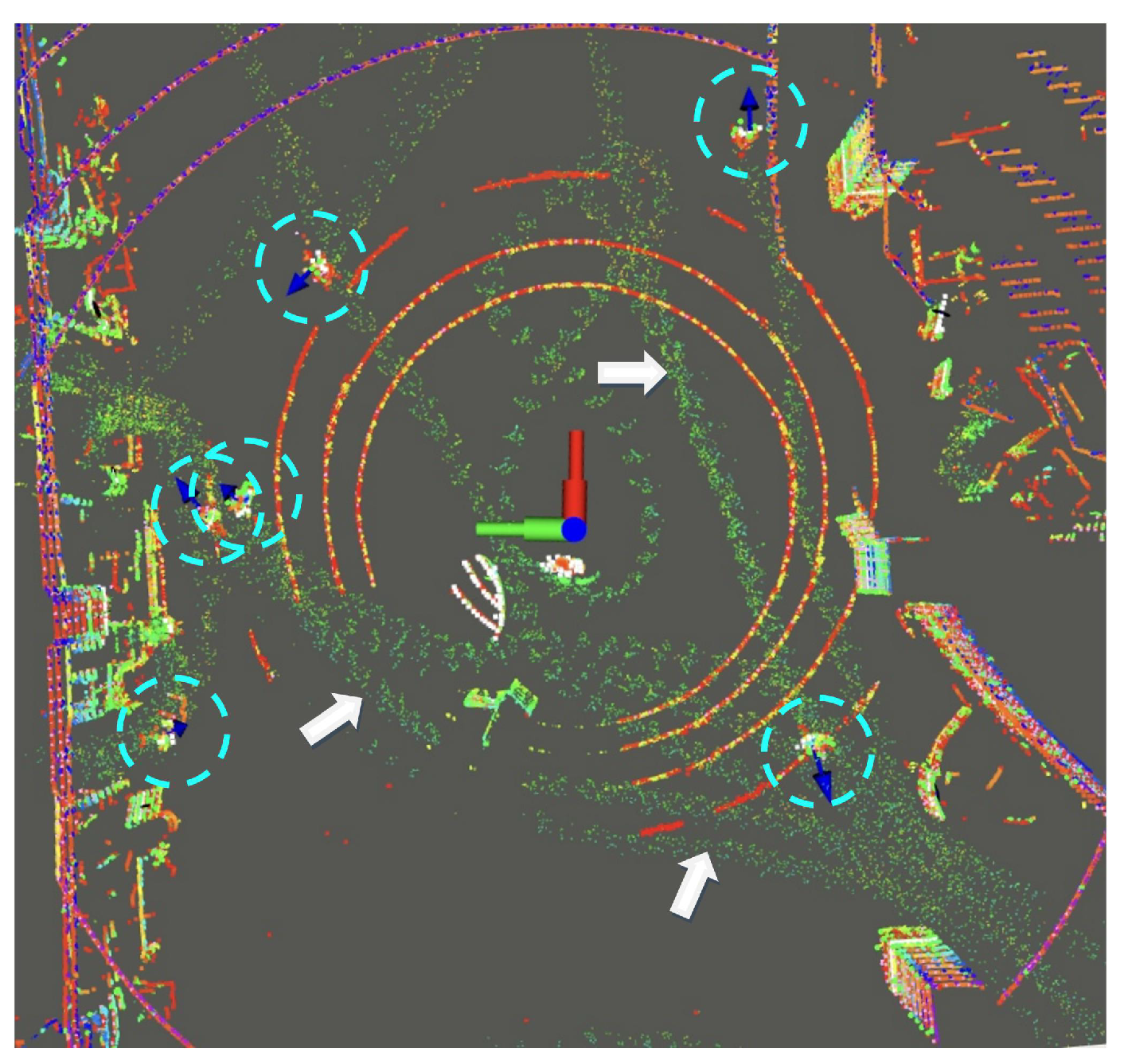
Figure 1. Multiple object tracking. The cyan circles highlight the positions and velocities of the targets. The white arrows indicate the traces of the targets in conventional SLAM.
Remotesensing 16 02622 g001
Figure 2. Overview of the proposed robot-based framework for the target activation map.
Remotesensing 16 02622 g002
Figure 3. Robot trajectory (blue solid line) and multiple target trajectories (dotted lines), with the latter including noise from static objects like walls and pillars. Each target trajectory is labeled with a number corresponding to a target ID and is colored sequentially to distinguish it.
Remotesensing 16 02622 g003
Figure 4. Robot trajectory (blue solid line) and dynamic target trajectories (dotted lines). Each target trajectory is labeled with a number corresponding to a target ID.
Remotesensing 16 02622 g004
Figure 5. (a) Result of grid cell algorithm. (b) Target activation map.
Remotesensing 16 02622 g005
Figure 6. Feature matching and Umeyama method result. The left part of (a) is the reference map, and the right part of (a) is the source map. The points matched in (a) are transformed to the metric scale and are represented as blue circle points and red triangle points, respectively, in (b). The source points transformed by the results of the Umeyama method, R and t , are depicted as yellow star points, indicating a proper transformation.
Remotesensing 16 02622 g006
Figure 7. Acquisition platform and environment. (a) Clearpath Jackal UGV in the indoor library [38]. (b) Floor guide of the library (c) Clearpath Husky UGV in the outdoor square. (d) Drone-captured image of the square [39].
Remotesensing 16 02622 g007
Figure 8. Experiment results for Library datasets. (a) Dynamic targets and robot trajectory. (b) Target activation map, where the grid cell size is 3 × 3 m and the lengthscale l = 2 for GPR. (c) Confidence map.
Remotesensing 16 02622 g008
Figure 9. Experiment results for Square datasets. (a) Dynamic targets and robot trajectory. (b) Target activation map, where the grid cell size is 3 × 3 m and the lengthscale l = 2.5 for GPR. (c) Confidence map.
Remotesensing 16 02622 g009
Figure 10. (a,c) The registered trajectories on reference maps for the Library and Square datasets, respectively. (b,d) The target activation maps, where (b) has a lengthscale l = 2 and (d) has a lengthscale l = 2.5 , both with a grid cell size of 3 × 3 m.
Remotesensing 16 02622 g010
Figure 11. OG map [41]. This map includes footprints of dynamic objects. The rectangles on the map highlight parts of these footprints.
Remotesensing 16 02622 g011
Figure 12. Paths according to each map: (a) Case 1: A path from the starting point to the endpoint that passes through all high-activity areas. (b) Case 2: A path to the highest activity level area.
Remotesensing 16 02622 g012
Table 1. Dataset summary: * indicates datasets that used a reference map.
DatasetDummy Target FilteringMapLength of Robot Trajectory (m)Time
Initial IDCountDynamic ID CountIn PixelsIn MetricResolution
Library_11412491368 × 105168.4 × 52.550.05347.39510 m 51 s
Library_2 *751181408 × 116672.45 × 51.35146.644 m 12 s
Library_3393101454 × 117772.7 × 58.8593.6413 m 48 s
Library_4591151250 × 111662.5 × 55.8115.2774 m 29 s
Library_5599181410 × 106070.55 × 53.3114.79516 m 10 s
Library_62024601450 × 105072.5 × 52.5359.21114 m 13 s
Library_7790231191 × 130459.55 × 65.2125.3165 m 23 s
Total6500203---1302.27549 m 11 s
Square_11147341783 × 163989.15 × 81.950.05346.73515 m 18 s
Square_21102281705 × 149385.25 × 74.65350.73615 m 37 s
Square_31496671946 × 189397.3 × 94.65345.12916 m 47 s
Square_4 *1323781800 × 175489.55 × 87.7353.52216 m 10 s
Total5068207---1396.12263 m 52 s
Table 2. Evaluation of activity levels and path lengths for paths generated using the A* algorithm across the TA map and OG maps for case 1 and case 2.
MetricOG Map [4]OG Map [41]TA Map
Case 1Activity
Level
Mean2.2992.1712.146
Variance3.7853.2622.984
Max7.8367.8465.500
Length of path (m)52.74755.18954.674
Case 2Activity
Level
Mean2.1312.1242.074
Variance4.1314.2293.701
Max7.8377.8477.847
Length of path (m)26.31726.40026.990
Disclaimer/Publisher’s Note: The statements, opinions and data contained in all publications are solely those of the individual author(s) and contributor(s) and not of MDPI and/or the editor(s). MDPI and/or the editor(s) disclaim responsibility for any injury to people or property resulting from any ideas, methods, instructions or products referred to in the content.