Article

Assessing Land Cover Classification Accuracy: Variations in Dataset Combinations and Deep Learning Models

1
Department of Forest Management, Division of Forest Sciences, College of Forest and Environmental Sciences, Kangwon National University, Chuncheon 24341, Republic of Korea
2
Forest ICT Research Center, National Institute of Forest Science, Seoul 02455, Republic of Korea
*
Author to whom correspondence should be addressed.
Remote Sens. 2024, 16(14), 2623; https://doi.org/10.3390/rs16142623
Submission received: 21 May 2024 / Revised: 30 June 2024 / Accepted: 15 July 2024 / Published: 18 July 2024

Abstract

:
This study evaluates land cover classification accuracy through adjustments to the deep learning model (DLM) training process, including variations in loss function, the learning rate scheduler, and the optimizer, along with diverse input dataset compositions. DLM datasets were created by integrating surface reflectance (SR) spectral data from satellite imagery with textural information derived from the gray-level co-occurrence matrix, yielding four distinct datasets. The U-Net model served as the baseline, with models A and B configured by adjusting the training parameters. Eight land cover classifications were generated from four datasets and two deep learning training conditions. Model B, utilizing a dataset comprising spectral, textural, and terrain information, achieved the highest overall accuracy of 90.3% and a kappa coefficient of 0.78. Comparing different dataset compositions, incorporating textural and terrain data alongside SR from satellite imagery significantly enhanced classification accuracy. Furthermore, using a combination of multiple loss functions or dynamically adjusting the learning rate effectively mitigated overfitting issues, enhancing land cover classification accuracy compared to using a single loss function.

1. Introduction

In 2016, the World Economic Forum brought attention to a new area of interest known as the Fourth Industrial Revolution. This has led to the global expectation of changes in the structure of industries as a result of the convergence of digital, biological, and physical technologies [1]. Following this, with the emergence of AlphaGo, discussions on elements of Fourth Industrial Revolution technology are ongoing worldwide.
In response to global trends, the Korea Forest Service created a strategic plan called the K-Forest Initiative. The goal of this initiative is to combine Fourth Industrial Revolution technologies with forestry research and development. The first step of this plan involves the implementation of digital and contactless technologies in the forestry sector [2]. Remote sensing is useful for implementing digital contactless technologies. This technology is beneficial for monitoring regions that are difficult to access, as well as large areas. It is expected to play a crucial role in understanding changes in land use, land cover, and forestry management activities [3,4]. The use of Fourth Industrial Revolution technologies and remote sensing can help improve the accuracy of the statistics on forests, as suggested by the Intergovernmental Panel on Climate Change (IPCC). The application of spatial approaches at the Tier 3 level is particularly effective for enhancing the accuracy of statistical information on greenhouse gases for climate change adaptation [5,6]. The IPCC proposed two approaches for developing national greenhouse gas statistics at the Tier 3 level: the sampling and wall-to-wall methods. The wall-to-wall method is particularly effective for accurately estimating spatial changes in land cover, making it suitable for advanced forest inventory estimations. The semantic segmentation-based deep learning model (DLM) was aligned with the wall-to-wall method [6].
DLMs based on semantic segmentation, including popular architectures such as U-Net, DeepLab, FCN, SegNet, and PSPNet, have been reported to exhibit high performance in land cover classification [7,8,9]. In studies on land cover classification using DLMs, researchers have sought to improve the model performance by adjusting the hyperparameters, input size, and input layers [10,11,12]. Remote-sensing data have certain limitations in distinguishing between land cover and land use, which can cause issues in accurately classifying similar land use categories. Some studies have compared different DLMs or investigated how the accuracy changes with variations in input information. Yuan et al. (2022) investigated the performance of various DLMs, including VGG, ResNet, Inception, and DenseNet, for land cover classification [13]. They emphasized the importance of selecting a model that is appropriate for the specific task of monitoring land cover changes. Despite the successful application of these DLMs, the efficiency and accuracy of deep learning-based land cover classification depend heavily on high-quality training data [14]. Lee and Lee (2022) reported that a lack of training data and data imbalance could degrade model performance [15]. Researchers have emphasized the importance of optimizing dataset composition and training conditions, including the application of data augmentation techniques and improvement of loss functions, for effective model development [16,17].
Therefore, this study aimed to assess the impact of deep learning model (DLM) training conditions and dataset compositions on the accuracy of land cover classification from satellite imagery. Unlike previous studies that often focus on either model architecture or dataset preparation, our research uniquely combines these aspects to provide a comprehensive analysis. We emphasize the significance of optimizing both learning conditions and dataset configurations over the architectural performance of DLMs in enhancing classification accuracy. This novel approach allows for the examination of optimization strategies for constructing reliable deep learning training models and improving classification accuracy across diverse land cover types. By systematically exploring the interplay between dataset composition, loss functions, and learning rate schedules, we aim to provide new insights into the development of more robust and accurate land cover classification models.

2. Materials and Methods

2.1. Study Area

The chosen study area is Chuncheon, the second-most populous city in the Gangwon Province, South Korea. Chuncheon is located within the longitude range of 127°30′22.12″E to 128°01′48.39″E and the latitude range of 37°40′28.28″N to 38°05′06.17″N (Figure 1). Chuncheon’s administrative division consists of one eup (town), nine myeons (townships), and 15 dongs (neighborhoods), covering an area of approximately 1120 km2 [18]. According to the statistics released by the Ministry of Land, Infrastructure, and Transport in 2023, the land use distribution in Chuncheon City is as follows: forests cover approximately 75%, making it the most extensive category. Wetlands and croplands accounted for 9.2 and 8.9%, respectively. Some changes in land use have occurred since 2013. Grasslands and wetlands have remained relatively stable, forests have decreased by 0.6%, and croplands decreased by 0.5%. However, artificial facilities such as residential areas have increased by 1.1% [19].

2.2. Research Method

In this study, a DLM was constructed for land cover classification by creating four datasets from satellite images using surface reflectance (SR) spectral and textural information (gray-level co-occurrence matrix, GLCM). U-Net architecture was used as the base model, and the learning conditions of the DLM were set by adjusting the loss function, learning rate scheduler, and optimizer. The main objective was to determine the optimal approach for land cover classification based on the learning conditions and dataset configurations of the DLM (Figure 2).

2.2.1. Construction of Datasets for Land-Use Categories Using Spectral and Textural Information

To apply a semantic segmentation-based DLM, it is essential to construct a dataset consisting of input images and corresponding label images, wherein the label images contain the true values for each pixel in the input images [20]. The input images comprised five SR images obtained from the RapidEye satellite imagery acquired on 21 May 2018, three textural features derived from SR information, and slope information derived from a digital elevation model (DEM). The label images used for training were provided by the Ministry of Environment and included detailed land cover classifications [21]. The RapidEye imagery, sourced from Planet Labs, Inc. (San Francisco, CA, USA), has a spatial resolution of 5 m and is composed of five spectral bands: red, green, blue, red edge, and near-infrared (NIR). Additionally, a GLCM was constructed using the NIR band information from RapidEye imagery. A GLCM is a statistical method used to analyze the texture of an image. It measures the relationship between pixels at specific distances and angles within an image. Several textural metrics can be derived from this analysis, including contrast, homogeneity, energy, entropy, and correlation. The textural features obtained from the GLCM can vary depending on the window size, quantization levels of input data, and distance and angle between pixels [22,23]. In this study, three textural features representing homogeneity, entropy, and correlation were utilized. Topographic information was obtained from the National Geographic Information Institute, and a DEM was constructed based on a 1:5000 topographic map. Subsequently, slope information was derived from DEM data. The label images used to represent the ground truth for the input images were created using the subdivision land cover map provided by the Ministry of the Environment. These data were further classified based on six land use categories defined by IPCC, including forest, cropland, grassland, wetland, settlement, and other land. Additionally, a Forest Management Activity Database obtained from the Korea Forest Service was used to create a spatial database of forestry-managed land. Article 3.4 of the Kyoto Protocol allows for the inclusion of greenhouse gas emissions or sequestration resulting from forest management activities in the calculation of national emissions. Consequently, spatial information from reforested and clear-cut areas in the Forest Management Activity Database was utilized as forestry-managed land information. Seven classification categories were used for the labeled images in the DLM (Figure 3) [24,25].
H o m o g e n e i t y = i = 0 N 1 i = 0 N 1 P i , j 1 + i j 2
E n t r o p y = i = 0 N 1 i = 0 N 1 P ( i , j ) l o g ( P ( i , j ) )
C o r r e l a t i o n = i = 0 N 1 i = 0 N 1 ( i μ x ) ( j μ x ) P ( i , j ) σ x σ x y
The input data consist of four datasets, all corresponding to the same location. These datasets are composed based on a combination of spectral, texture, and terrain information. Dataset A comprised five pieces of spectral information from RapidEye imagery. Dataset B was composed of spectral information combined with three pieces of textural information. Dataset C used both spectral and terrain information, specifically slope. Dataset D incorporated spectral, textural, and slope information (Table 1). These datasets were classified into training data for the learning process of the DLM, validation data for improving the accuracy of the model during training, and testing data for applying the trained DLM. The image size of the dataset was set to 256 × 256 pixels. The input and label images were divided into tile-shaped images of this size. Tiled images representing approximately 10% of each study area were selected using random sampling. These images were then utilized in a 7:3 ratio as training and validation data. To address the issue of decreased classification accuracy at the outer edges of images in the deep learning model (DLM), the test data, consisting of entire tile images of the study area, were constructed with a 50% overlap rate.

2.2.2. Building and Configuring Deep Learning Models for Land Cover Classification

We chose the U-Net model as the foundational architecture for land cover classification. The U-Net model incorporates an encoder and decoder structure, with the encoder featuring U-Net blocks consisting of two convolutional layers for extracting feature information from images. The model follows a simple design with four repeated down-sampling operations, making it effective for semantic segmentation tasks. In the decoder, up-sampling was performed four times through repeated operations to restore the reduced-size images from the down-sampling to their original resolution. In addition, after each up-sampling operation, skip connections were utilized to prevent issues related to information loss and gradient vanishing by incorporating the feature information from each layer of the encoder (Figure 4). While the U-Net model was developed in 2015, its efficient architecture has led to the utilization of numerous derivative models, such as ResU-Net, U-Net++, Attention U-Net, and TransU-Net [26,27,28,29,30].
The training of a DLM commences by initializing all weights with small random values. The output was generated as training data that passed through each layer of the model. The loss function computed the difference between the predicted and actual values. The goal was to minimize the loss, which was achieved by calculating the gradient of the loss with respect to each weight and updating the weights accordingly. The DLM repeats the training process for a defined number of epochs and adjusts the weights based on training and validation data to minimize the loss between the predicted and actual values [31,32]. The learning rate of the DLM can be set using a fixed learning rate through a learning rate scheduler or by gradually decreasing or increasing. The optimizer updates the weights accordingly. In this study, we focused on improving the accuracy of a DLM by adjusting key parameters such as the loss function, learning rate scheduler, and optimizer. Training Model A used the cross-entropy loss function and Adam optimizer for semantic segmentation. The learning rate scheduler started at 0.01 and decreased progressively with each epoch. Training model B uses the hybrid loss function and AdamW optimizer, with the learning rate managed dynamically using the OneCycleLR technique. The hybrid loss function is a combination of three loss functions, including multiscale structural similarity, focal loss, and dice loss. the OneCycleLR technique is widely known for its effectiveness in addressing issues related to dataset imbalance and overfitting [33,34]. The DLM was trained for a maximum of 1000 epochs. To evaluate the model’s performance, the training was repeated ten times under the same conditions to assess consistency.

2.2.3. Evaluation of Consistency for Deep Learning-Based Land Cover Maps

A trained DLM was used to create a land cover map. The accuracy of the deep learning-based classification of land cover was evaluated by comparing the maps with label images. To evaluate the accuracy of the deep learning-based classification of land cover, a confusion matrix was created and used to calculate the overall accuracy and kappa coefficient (Table 2) [35,36]. Precision and recall were calculated for each land cover category, and the F1-score was used to assess the classification accuracy for different categories of land cover. To calculate OA, Kappa, and F1-Score, the metrics True Positive (TP), True Negative (TN), False Positive (FP), and False Negative (FN) are utilized. TP refers to the instances correctly identified as positive, TN indicates instances correctly identified as negative, FP represents instances incorrectly identified as positive, and FN denotes instances incorrectly labeled as negative, serving as fundamental components in evaluating the performance of classification models by distinguishing between accurately and inaccurately classified instances.
O v e r a l l   A c c u r a c y = T P + T N T P + T N + F P + F N
K a p p a = O A p e 1 p e
p e = T P + F N T P + F N + F P + T N × T P + F P T P + F N + F P + T N + F P + T N T P + F N + F P + T N × F N + T N T P + F N + F P + T N
P r e c i s i o n = T P T P + F P
R e c a l l = T P T P + F N
F 1 s c o r e = 2 × P r e c i s i o n × R e c a l l P r e c i s i o n + R e c a l l

3. Results and Discussion

3.1. Distribution Patterns of Area Ratios, Surface Reflectance, and GLCM across Land Cover Categories in Deep Learning Training Data

The deep learning dataset was constructed with a window size of 256 × 256 pixels, comprising 113 training and 47 validation images. The land cover distribution in the training dataset showed that forests accounted for 64.5% of the total area, followed by wetlands, grasslands, croplands, settlements, and forestry-managed lands. Forestry-managed lands and other land accounted for <2% of the total area of the training dataset.
When comparing the SR distribution across categories in the training dataset, the SR values in the red band were the highest for other lands, settlements, and croplands. However, in the NIR band, the SR values were the highest in forests, grasslands, and forestry-managed lands. The distribution characteristics of forests and wetlands were distinctly different from those of other categories. However, the distribution patterns of croplands, settlements, and other land types were similar. The distribution characteristics of other lands encompassed a wide range, including croplands and settlements. Croplands, especially those included in the detailed category of facility cultivation (greenhouse cultivation areas), showed a high degree of overlap with settlements.
When comparing the distribution characteristics of the GLCM across categories, the entropy of GLCM showed similarity across all categories, while the homogeneity values of the GLCM in wetlands were 1.7 times higher than those in other categories. Additionally, the correlation of GLCM showed mostly negative values across categories, whereas other lands and forestry-managed lands showed positive values. Moreover, the correlation of the GLCM displayed varied distributions based on land cover categories, indicating that it is considered the most suitable information within the GLCM for land cover classification. When comparing the distribution characteristics of slopes across categories, forests and forestry-managed lands were distributed across regions with high slopes. By contrast, wetlands and croplands were relatively distributed in areas with low slopes (Table 3).

3.2. Comparison of Training and Validation Accuracy in Deep Learning Model for Land Cover Classification

The training and validation accuracy of the DLM were assessed based on 10 repeated training sessions at 1000 epochs. Table 4 shows the average values obtained from 10 repeated training sessions. For Model A, training exhibited a high accuracy of >90%. However, the validation accuracy was approximately 10% lower than that of training, indicating signs of overfitting. By contrast, for Model B, both the training and validation accuracies showed a minimal difference of approximately 1%, and the validation accuracy was distributed at 3–5% higher than that of Model A. A comparison of the results of the two models showed that employing a combination of multiple loss functions and dynamically adjusting the learning rate was advantageous for preventing overfitting as opposed to using a single loss function and a fixed learning rate. In particular, the dataset used in this study showed an imbalanced distribution, with forests having the widest coverage, while the remaining categories were smaller. While the loss distribution of Model B was higher than that of Model A, both training and validation accuracies remained relatively stable compared to Model A. Similar to the results of previous studies, it was deemed effective to apply hybrid loss functions that combine three loss functions for imbalanced datasets [37,38,39,40]. When comparing the differences in training and validation accuracy across datasets, Model A achieved the highest training and validation accuracies when utilizing only the spectral information from Dataset A. However, when textural and slope information were added, the accuracy decreased. For Model B, adding textural information to the spectral information in Dataset B decreased the training and validation accuracies. However, when slope information was added to Dataset C, and textural and slope information were included in Dataset D, the accuracies were the highest. The highest accuracy observed in Model A when solely utilizing spectral information may be attributed to variations in training methodologies. Model B improved its generalization capability through a hybrid loss strategy that concurrently considers multiple types of losses and an enhanced AdamW that reduces weight decay and restrains overfitting. Consequently, Model B, which is equipped with a sophisticated algorithm designed to process more complicated and diverse information, achieves the highest accuracy when it utilizes a combination of spectral, textural, and slope data. Model A, by contrast, shows the opposite results. The training time for deep learning models varied by dataset, with Dataset A requiring the shortest average training time of approximately 127 min. When textural or slope information was incorporated into the input images, an additional training time of approximately 4–5 min was necessary.

3.3. Evaluation of Land Cover Classification Accuracy for Each Deep Learning Model

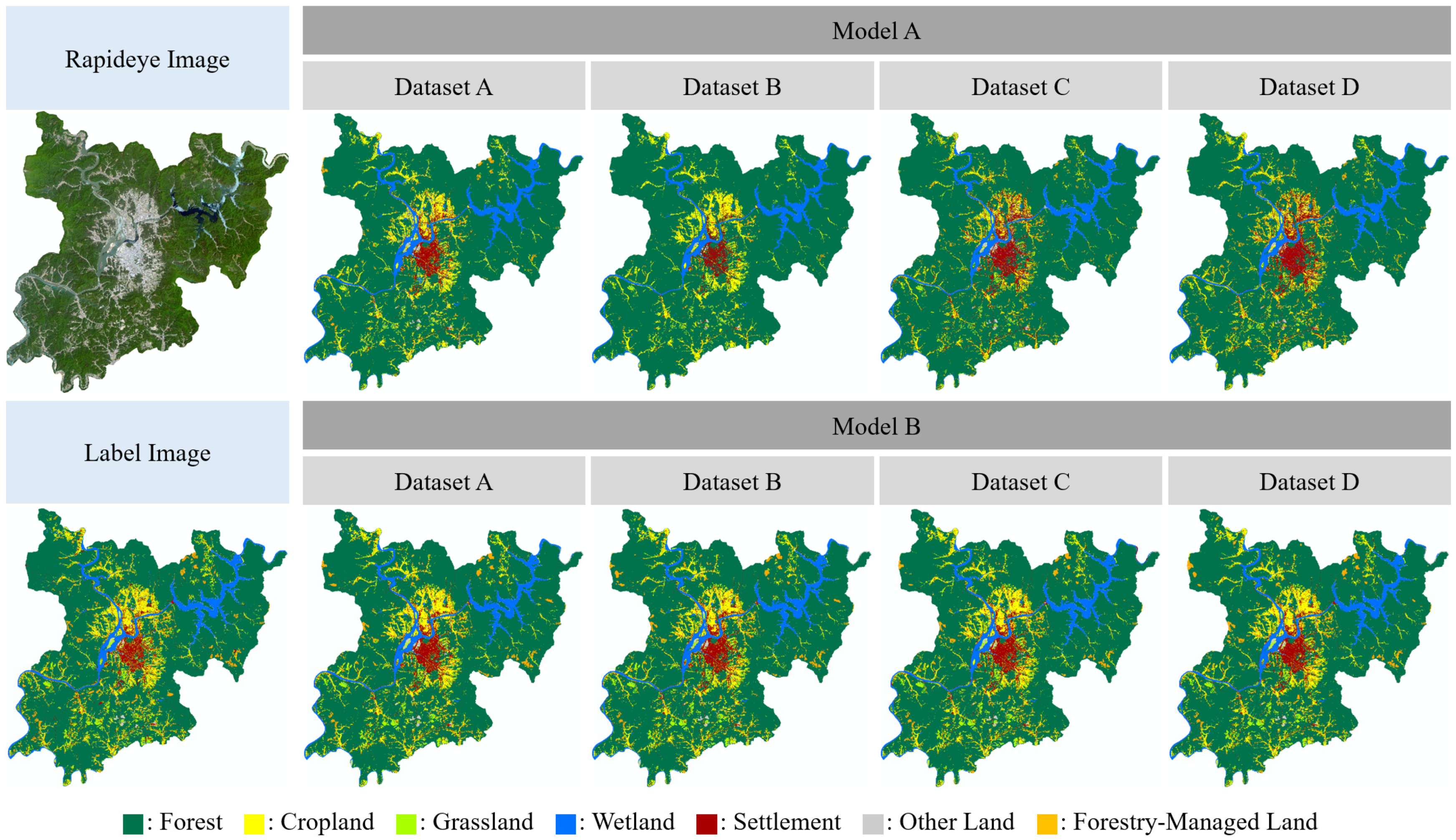
Figure 5 shows the results of land cover mapping based on the trained DLM. A comparison between the label image and the land cover map generated by the DLMs showed that for Model A, the use of Dataset A resulted in the highest accuracy with an average kappa value of 0.71. Conversely, for Model B, the use of Dataset D yielded the highest accuracy, with an average kappa value of 0.77. The incorporation of textural and slope information alongside spectral data yielded contrasting results in Models A and B. In Model A, this addition led to a decrease in both Overall Accuracy (OA) and Kappa coefficients. Conversely, Model B demonstrated a slight enhancement in both OA and Kappa values upon the inclusion of textural and slope information (Table 5). Previous studies have reported that the use of a combination of spectral, terrain, and GLCM information is effective in improving the accuracy of image classification [41,42,43]. In reviewing research on land cover classification using the U-Net model, Giang et al. (2020) [44] achieved a maximum Overall Accuracy (OA) of approximately 84.8% in their study on land cover classification using the U-Net model based on UAV imagery. Similarly, Kim et al. (2021) [45] reported a maximum OA of approximately 84.6% in their research on land cover classification utilizing the U-Net model with Sentinel-2 satellite imagery. By contrast, the DLM trained in this study attained a maximum OA of approximately 90.4%, demonstrating higher accuracy than previous studies. This improvement in accuracy is attributed to the additional use of the GLCM and slope information, as well as optimization of the training process through the use of a hybrid loss function [44,46].
Applying hybrid loss and dynamic learning rate methods improved the accuracy of the kappa coefficient by approximately 0.06 compared to the application of a single loss function and a fixed learning rate. Nanni et al. (2021) [47] and Huang et al. (2020) [40] reported improvements in accuracy by combining multiple loss functions compared with using a single loss function, which is consistent with the results of this study. Llugsi et al. (2021) reported a decrease in the mean-squared error when using AdamW as the optimizer instead of Adam [48]. Considering these results collectively, it can be concluded that, while the composition of the dataset influences accuracy improvement, the configuration of deep learning training conditions, including loss functions, optimizers, and learning rate schedules, has a more significant impact on accuracy.

3.4. Comparison of Land Cover Accuracy between Deep Learning Model and Label Images by Categories

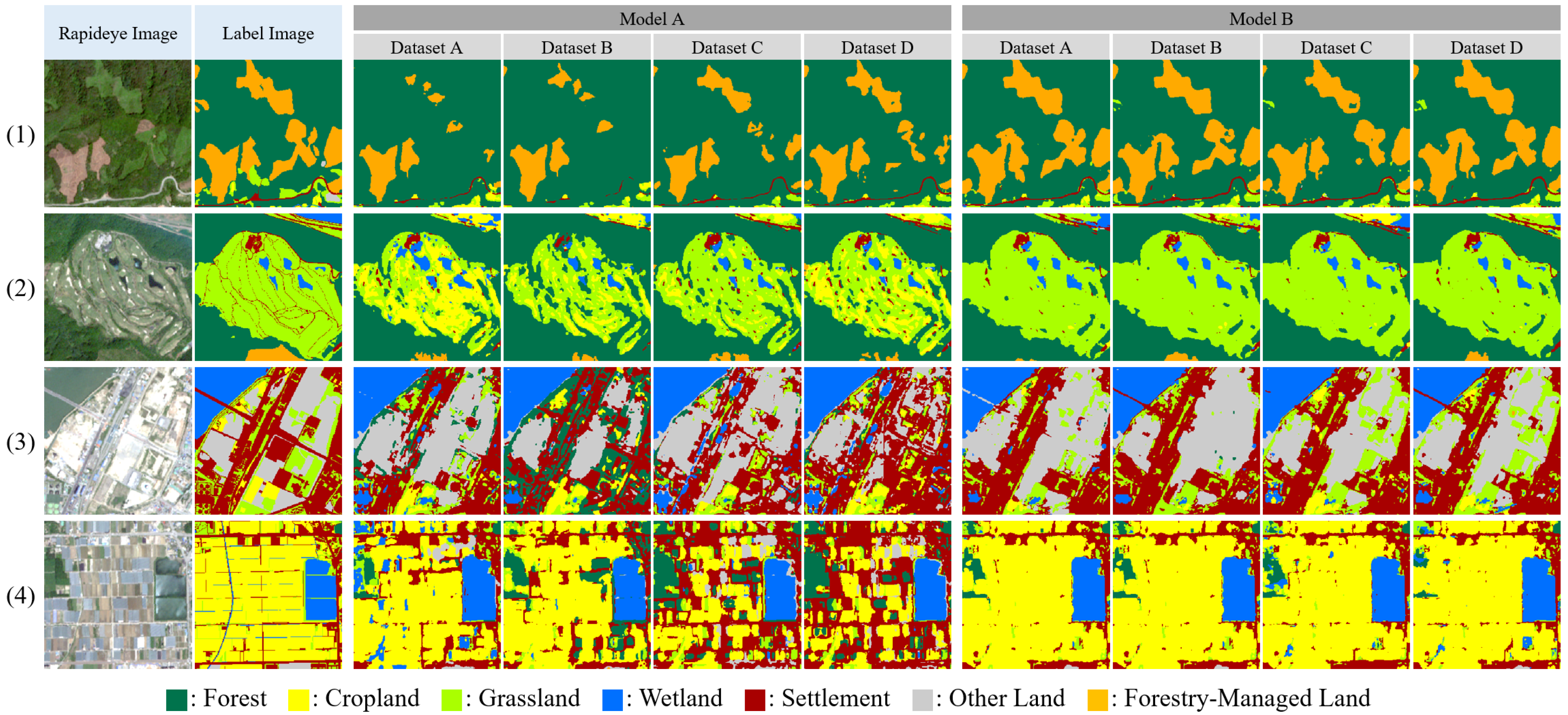
When comparing the land cover maps generated by the DLM labeled images, we found that in Model A, forests were overestimated by an average of 6.3%, grasslands were underestimated by 3.2%, and forestry-managed lands were underestimated by 1.2%. By contrast, Model B showed area distribution rates for all categories within a 1% similarity to the label image. When comparing the accuracy of land cover classification by category, regardless of the dataset composition, both Models A and B showed a high accuracy of approximately 87% or higher for forests and wetlands, showing a trend similar to those of previous research [49,50]. Similar to previous studies, grassland and other land categories showed lower accuracies than those of the other categories [15,51]. When comparing the accuracy of land cover categories based on each DLM, Models A and B showed similar F1-score distributions for the forest and wetland categories. However, when using Model B, the accuracy of categories such as forestry-managed land, grassland, other land, and cropland showed significant improvements (Figure 6).
The F1-score showed the most significant improvement in the forestry-managed land, reaching an average of 21.2%. In Model A, numerous cases of misclassification of forestry-managed lands as forests were observed (Figure 7(1)). Grassland areas are primarily distributed within golf courses and urban parks. While Model A exhibited numerous cases of misclassification of grasslands as forests and croplands, Model B showed a distribution more similar to that of the label image (Figure 7(2)). Other land categories within the study area corresponded to quarries, developing land, and bare land, exhibiting spectral characteristics similar to those of the settlements. Therefore, numerous cases of misclassification between settlements and other land categories were observed (Figure 7(3)). Croplands include cultivated areas, such as rice paddies, fields, and orchards. In Model A, numerous misclassifications in regions with spectral characteristics similar to those of the settlements, such as greenhouse cultivation and glass greenhouses, were observed. On the other hand, Model B exhibited a distribution similar to the label image but misclassified areas such as orchards as forests (Figure 7(4)). Misclassification instances were predominantly distributed among categories with similar spectral characteristics, such as forest ↔ forestry-managed lands, cropland ↔ grassland, and cropland (facility cultivation areas) ↔ settlements. The improved learning conditions of Model B led to a decrease in misclassification cases. However, detecting small-sized roads and objects remained a challenge.
To solve these issues, several solutions can be considered, including the application of augmentation techniques, improvement in model architecture, and implementation of post-processing methods. Zhang et al. (2021) reported that augmentation techniques such as scaling, movement, and rotation can enhance the generalization performance of models and suggested ObjectAug, an object-level augmentation technique [52]. Furthermore, misclassification rates could be improved if the structure of models using multi-scale filters or self-attention mechanisms such as Transformers is applied to deep learning models, which can facilitate the extraction of diverse feature information [53,54]. The application of post-processing techniques such as Conditional Random Fields (CRFs) or Graph Cut can refine classification results. Wang et al. (2022) demonstrated that applying CRF to deep learning models reduces isolated small patches and improves classification accuracy [55]. To improve accuracy and reduce misclassification in land cover maps, these methods should be explored.

3.5. Utilization of Land Cover Maps Based on Deep Learning Models

Information on land cover changes is essential for resource management, urban planning, and disaster assessment. Land cover classification and change detection are crucial tasks in the field of remote sensing, so they have been extensively studied over the past few decades [56]. In particular, the IPCC requires all parties to report the changes in land use by category over the past 20 years to compile greenhouse gas absorption and emission statistics for the Land Use, Land-Use Change and Forestry (LULUCF) sector [25]. Applying deep learning techniques to time-series imagery allows for the construction of time-series land cover maps, which can be an effective means of annually estimating large-scale land use changes. In South Korea, the land cover map developed by the Ministry of Environment was designated as a nationally approved statistic, and it provides annual land cover statistics [57]. The methods used in this study are considered beneficial for training deep learning models with large datasets and can serve as fundamental data for calculating time-series land cover changes.
Additionally, deep learning-based land cover maps play a significant role in urban planning, landscaping, and the development of environmental scenarios. Mahmoudzadeh et al. (2022) predicted urban growth rates and proposed an ecological development framework based on historical land use and land cover data [58]. Similarly, Mehra and Swain (2024) forecasted future land cover conditions using past land cover information and suggested management strategies for addressing socio-ecological and environmental issues [59]. In this way, land cover maps are utilized in various applications, such as analyzing current land use statuses, designating redevelopment and conservation areas, managing and designing green spaces, and preparing for natural disasters. This multifaceted application enables the formulation of effective planning strategies.

4. Conclusions

This study explored the best land cover classification methods using DLMs. It examined the effects of loss functions, learning rate schedulers, optimizers, and dataset compositions on the training process. The DLM for land cover classification is more effective when the dataset includes both SR information from satellite imagery and textural information or terrain features. Utilizing multiple loss functions or dynamically adjusting the learning rate is considered effective, particularly in scenarios where training data are unevenly distributed, ultimately enhancing both training and validation accuracy. The forests in the land cover maps generated by the DLMs in this study exhibited excellent classification accuracy, exceeding 97%. These models hold significant value in constructing land-use change matrices for greenhouse gas inventories. However, grasslands and other land types consistently exhibited accuracies below 50% across all models due to insufficient training data, limitations in distinguishing between land cover and land use, and errors introduced by the diversity of subcategories within land-use categories. The integration of spatial information is necessary to address these limitations and further improve model accuracy.
Our study makes several novel contributions to the field of land cover classification using deep learning. Firstly, we demonstrate that the combination of multiple loss functions and dynamic learning rate adjustments significantly enhances classification accuracy, particularly for imbalanced datasets. This finding addresses a common challenge in remote sensing applications where certain land cover types are underrepresented. Secondly, our comprehensive analysis of various dataset compositions reveals that integrating spectral, textural, and terrain information yields the best classification results, providing a new benchmark for dataset preparation in land cover studies. Lastly, our approach of systematically evaluating both model training conditions and input data characteristics offers a novel framework for optimizing deep learning models in remote sensing applications. These insights not only advance the theoretical understanding of deep learning in land cover classification but also provide practical guidelines for improving the accuracy and reliability of large-scale land use change assessments, crucial for environmental monitoring and urban planning.

Author Contributions

Conceptualization, W.-D.S. and J.-S.L.; Methodology, W.-D.S. and J.-S.L.; Software, W.-D.S.; Validation, W.-D.S. and J.-S.L.; Formal Analysis, W.-D.S.; Investigation, W.-D.S.; Resources, W.-D.S.; Data Curation, W.-D.S. and J.-S.Y.; Writing—Original Draft Preparation, W.-D.S.; Writing—Review and Editing, J.-S.Y. and J.-S.L.; Visualization, W.-D.S.; Supervision, J.-S.Y. and J.-S.L.; Project Administration, J.-S.L.; Funding Acquisition, J.-S.L. All authors have read and agreed to the published version of the manuscript.

Funding

This research was funded by the Korea National Institute of Forest Science under project FM 0103-2021-04-2024.

Data Availability Statement

The original contributions presented in the study are included in the article, further inquiries can be directed to the corresponding author.

Conflicts of Interest

The authors declare no conflicts of interest.

References

  1. Schwab, K. The Fourth Industrial Revolution; Currency: New York, NY, USA, 2017; Available online: https://play.google.com/store/books/details?id=ST_FDAAAQBAJ (accessed on 2 February 2024).
  2. KFS (Korea Forest Service). K-Forest. Available online: https://www.forest.go.kr/kfsweb/kfi/kfs/cms/cmsView.do?mn=NKFS_02_13_04&cmsId=FC_003420 (accessed on 2 February 2024).
  3. Kim, E.S.; Won, M.; Kim, K.; Park, J.; Lee, J.S. Forest management research using optical sensors and remote sensing technologies. Korean J. Remote Sens. 2019, 35, 1031–1035. [Google Scholar] [CrossRef]
  4. Woo, H.; Cho, S.; Jung, G.; Park, J. Precision forestry using remote sensing techniques: Opportunities and limitations of remote sensing application in forestry. Korean J. Remote Sens. 2019, 35, 1067–1082. [Google Scholar] [CrossRef]
  5. Lee, W.K.; Kim, M.; Song, C.; Lee, S.G.; Cha, S.; Kim, G. Application of Remote Sensing and Geographic Information System in Forest Sector. J. Cadastre Land InformatiX 2016, 46, 27–42. [Google Scholar] [CrossRef]
  6. Park, E.B.; Song, C.H.; Ham, B.Y.; Kim, J.W.; Lee, J.Y.; Choi, S.E.; Lee, W.K. Comparison of sampling and wall-to-wall methodologies for reporting the GHG inventory of the LULUCF sector in Korea. J. Climate Chang. Res. 2018, 9, 385–398. [Google Scholar] [CrossRef]
  7. Cho, K.; Van Merriënboer, B.; Gulcehre, C.; Bahdanau, D.; Bougares, F.; Schwenk, H.; Bengio, Y. Learning phrase representations using RNN encoder-decoder for statistical machine translation. arXiv 2014. [Google Scholar] [CrossRef]
  8. Solórzano, J.V.; Mas, J.F.; Gao, Y.; Gallardo-Cruz, J.A. Land use land cover classification with U-net: Advantages of combining sentinel-1 and sentinel-2 imagery. Remote Sens. 2021, 13, 3600. [Google Scholar] [CrossRef]
  9. Son, S.; Lee, S.H.; Bae, J.; Ryu, M.; Lee, D.; Park, S.R.; Seo, D.; Kim, J. Land-cover-change detection with aerial orthoimagery using segnet-based semantic segmentation in Namyangju City, South Korea. Sustainability 2022, 14, 12321. [Google Scholar] [CrossRef]
  10. Lee, Y.; Sim, W.; Park, J.; Lee, J. Evaluation of hyperparameter combinations of the U-net model for land cover classification. Forests 2022, 13, 1813. [Google Scholar] [CrossRef]
  11. Yaloveha, V.; Podorozhniak, A.; Kuchuk, H. Convolutional neural network hyperparameter optimization applied to land cover classification. Radioelectron. Comput. Syst. 2022, 23, 115–128. [Google Scholar] [CrossRef]
  12. Azedou, A.; Amine, A.; Kisekka, I.; Lahssini, S.; Bouziani, Y.; Moukrim, S. Enhancing land cover/land use (LCLU) classification through a comparative analysis of hyperparameters optimization approaches for deep neural network (DNN). Ecol. Inf. 2023, 78, 102333. [Google Scholar] [CrossRef]
  13. Yuan, J.; Ru, L.; Wang, S.; Wu, C. WH-MAVS: A novel dataset and deep learning benchmark for multiple land use and land cover applications. IEEE J. Sel. Top. Appl. Earth Obs. Remote Sens. 2022, 15, 1575–1590. [Google Scholar] [CrossRef]
  14. Zhang, X.; Han, L.; Han, L.; Zhu, L. How well do deep learning-based methods for land cover classification and object detection perform on high resolution remote sensing imagery? Remote Sens. 2020, 12, 417. [Google Scholar] [CrossRef]
  15. Lee, S.H.; Lee, M.J. A study on deep learning optimization by land cover classification item using satellite imagery. Korean J. Remote Sens. 2020, 36, 1591–1604. [Google Scholar] [CrossRef]
  16. Jeong, M.; Choi, H.; Choi, J. Analysis of change detection results by UNet++ models according to the characteristics of loss function. Korean J. Remote Sens. 2020, 36, 929–937. [Google Scholar] [CrossRef]
  17. Baek, W.K.; Lee, M.J.; Jung, H.S. The performance improvement of U-Net model for landcover semantic segmentation through data augmentation. Korean J. Remote Sens. 2022, 38, 1663–1676. [Google Scholar] [CrossRef]
  18. Chuncheon-si. Introduce Chuncheon. Available online: https://www.chuncheon.go.kr/cityhall/about-chuncheon/introduction/general/ (accessed on 2 February 2024).
  19. Ministry of Land, Infrastructure and Transport. Cadastral Statistics. Available online: https://stat.molit.go.kr/portal/cate/statMetaView.do?hRsId=24 (accessed on 2 February 2024).
  20. Géron, A. Hands-on Machine Learning with Scikit-Learn, Keras, and TensorFlow; O’Reilly Media, Inc.: Sebastopol, CA, USA, 2022; Available online: https://dl.acm.org/doi/abs/10.5555/3378999 (accessed on 2 February 2024).
  21. Ministry of Environment. Land Cover Map. Available online: https://egis.me.go.kr/intro/land.do (accessed on 2 February 2024).
  22. Haralick, R.M.; Shanmugam, K.; Dinstein, I.H. Textural features for image classification. IEEE Trans. Syst. Man Cybern. 1973, 6, 610–621. [Google Scholar] [CrossRef]
  23. Clausi, D.A. An analysis of co-occurrence texture statistics as a function of grey level quantization. Can. J. Remote Sens. 2002, 28, 45–62. [Google Scholar] [CrossRef]
  24. Kyoto Protocol. Kyoto Protocol. UNFCCC Website. Available online: http://unfccc.int/kyoto_protocol/items/2830.php (accessed on 2 February 2024).
  25. Intergovernmental Panel on Climate Change. 2006 IPCC Guidelines for National Greenhouse Gas Inventories; Institute for Global Environmental Strategies: Hayama, Kanagawa, Japan, 2006; Available online: http://www.ipcc-nggip.iges.or.jp/ (accessed on 2 February 2024).
  26. Ronneberger, O.; Fischer, P.; Brox, T. U-net: Convolutional networks for biomedical image segmentation. In Medical Image Computing and Computer-Assisted Intervention–MICCAI 2015: 18th International Conference, Munich, Germany, October 5–9, 2015, Proceedings, Part III 18; Springer International Publishing: Berlin/Heidelberg, Germany, 2015; pp. 234–241. [Google Scholar] [CrossRef]
  27. Oktay, O.; Schlemper, J.; Folgoc, L.L.; Lee, M.; Heinrich, M.; Misawa, K.; Mori, K.; McDonagh, S.; Hammerla, N.Y.; Kainz, B.; et al. Attention u-net: Learning where to look for the pancreas. arXiv 2018. [Google Scholar] [CrossRef]
  28. Zhang, Z.; Liu, Q.; Wang, Y. Road extraction by deep residual u-net. IEEE Geosci. Remote Sens. Lett. 2018, 15, 749–753. [Google Scholar] [CrossRef]
  29. Zhou, Z.; Rahman Siddiquee, M.M.; Tajbakhsh, N.; Liang, J. Unet++: A nested u-net architecture for medical image segmentation. In Deep Learning in Medical Image Analysis and Multimodal Learning for Clinical Decision Support: 4th International Workshop, DLMIA 2018, and 8th International Workshop, ML-CDS 2018, Held in Conjunction with MICCAI 2018, Granada, Spain, September 20, 2018, Proceedings 4; Springer International Publishing: Berlin/Heidelberg, Germany, 2018; pp. 3–11. [Google Scholar] [CrossRef]
  30. Chen, J.; Lu, Y.; Yu, Q.; Luo, X.; Adeli, E.; Wang, Y.; Lu, L.; Yuille, A.L.; Zhou, Y. Transunet: Transformers make strong encoders for medical image segmentation. arXiv 2021. [Google Scholar] [CrossRef]
  31. Rumelhart, D.E.; Hinton, G.E.; Williams, R.J. Learning representations by back-propagating errors. Nature 1986, 323, 533–536. [Google Scholar] [CrossRef]
  32. Kingma, D.P.; Ba, J. Adam: A method for stochastic optimization. arXiv 2014. [Google Scholar] [CrossRef]
  33. Loshchilov, I.; Hutter, F. Fixing Weight Decay Regularization in Adam. Available online: https://openreview.net/forum?id=rk6qdGgCZ (accessed on 2 February 2024).
  34. Smith, L.N.; Topin, N. Super-convergence: Very fast training of neural networks using large learning rates. In Artificial Intelligence and Machine Learning for Multi-Domain Operations Applications; SPIE: New York, NY, USA, 2019; Volume 11006, pp. 369–386. [Google Scholar] [CrossRef]
  35. Rouhi, R.; Jafari, M.; Kasaei, S.; Keshavarzian, P. Benign and malignant breast tumors classification based on region growing and CNN segmentation. Expert Syst. Appl. 2015, 42, 990–1002. [Google Scholar] [CrossRef]
  36. Huang, M.H.; Rust, R.T. Artificial intelligence in service. J. Serv. Res. 2018, 21, 155–172. [Google Scholar] [CrossRef]
  37. Wang, Z.; Simoncelli, E.P.; Bovik, A.C. Multiscale structural similarity for image quality assessment. In Proceedings of the Thirty-Seventh Asilomar Conference on Signals, Systems & Computers, Pacific Grove, CA, USA, 9–12 November 2003; IEEE: Piscataway, NJ, USA, 2003; Volume 2, pp. 1398–1402. [Google Scholar] [CrossRef]
  38. Milletari, F.; Navab, N.; Ahmadi, S.A. V-net: Fully convolutional neural networks for volumetric medical image segmentation. In Proceedings of the 2016 Fourth International Conference on 3D Vision (3DV), Stanford, CA, USA, 25–28 October 2016; IEEE: Piscataway, NJ, USA, 2016; pp. 565–571. [Google Scholar] [CrossRef]
  39. Lin, T.Y.; Goyal, P.; Girshick, R.; He, K.; Dollár, P. Focal loss for dense object detection. In Proceedings of the IEEE International Conference on Computer Vision, Venice, Italy, 22–29 October 2017; IEEE: Piscataway, NJ, USA, 2017; pp. 2980–2988. Available online: https://openaccess.thecvf.com/content_iccv_2017/html/Lin_Focal_Loss_for_ICCV_2017_paper.html (accessed on 2 February 2024).
  40. Huang, H.; Lin, L.; Tong, R.; Hu, H.; Zhang, Q.; Iwamoto, Y.; Han, X.; Chen, Y.W.; Wu, J. Unet 3+: A full-scale connected unet for medical image segmentation. In Proceedings of the ICASSP 2020—2020 IEEE International Conference on Acoustics, Speech and Signal Processing (ICASSP), Virtual, 4–9 May 2020; IEEE: Piscataway, NJ, USA, 2020; pp. 1055–1059. [Google Scholar] [CrossRef]
  41. Yu, L.; Su, J.; Li, C.; Wang, L.; Luo, Z.; Yan, B. Improvement of moderate resolution land use and land cover classification by introducing adjacent region features. Remote Sens. 2018, 10, 414. [Google Scholar] [CrossRef]
  42. Zheng, X.; Han, L.; He, G.; Wang, N.; Wang, G.; Feng, L. Semantic segmentation model for wide-area coseismic landslide extraction based on embedded multichannel spectral–topographic feature fusion: A case study of the Jiu-zhaigou Ms7.0 earthquake in Sichuan, China. Remote Sens. 2023, 15, 1084. [Google Scholar] [CrossRef]
  43. Li, W.; Li, Y.; Gong, J.; Feng, Q.; Zhou, J.; Sun, J.; Shi, C.; Hu, W. Urban water extraction with UAV high-resolution remote sensing data based on an improved U-Net model. Remote Sens. 2021, 13, 3165. [Google Scholar] [CrossRef]
  44. Giang, T.L.; Dang, K.B.; Le, Q.T.; Nguyen, V.G.; Tong, S.S.; Pham, V.M. U-Net convolutional networks for mining land cover classification based on high-resolution UAV imagery. IEEE Access 2020, 8, 186257–186273. [Google Scholar] [CrossRef]
  45. Kim, J.; Lim, C.H.; Jo, H.W.; Lee, W.K. Phenological classification using deep learning and the sentinel-2 satellite to identify priority afforestation sites in North Korea. Remote Sens. 2021, 13, 2946. [Google Scholar] [CrossRef]
  46. Ulmas, P.; Liiv, I. Segmentation of satellite imagery using u-net models for land cover classification. arXiv 2020. [Google Scholar] [CrossRef]
  47. Nanni, L.; Cuza, D.; Lumini, A.; Loreggia, A.; Brahnam, S. Deep ensembles in bioimage segmentation. arXiv 2021. [Google Scholar] [CrossRef]
  48. Llugsi, R.; El Yacoubi, S.; Fontaine, A.; Lupera, P. Comparison between Adam, AdaMax and Adam W optimizers to implement a weather forecast based on neural networks for the Andean city of Quito. In Proceedings of the 2021 IEEE Fifth Ecuador Technical Chapters Meeting (ETCM), Cuenca, Spain, 12–15 October 2021; IEEE: Piscataway, NJ, USA, 2021; pp. 1–6. [Google Scholar] [CrossRef]
  49. Zhang, P.; Ke, Y.; Zhang, Z.; Wang, M.; Li, P.; Zhang, S. Urban land use and land cover classification using novel deep learning models based on high spatial resolution satellite imagery. Sensors 2018, 18, 3717. [Google Scholar] [CrossRef] [PubMed]
  50. Han, Z.; Dian, Y.; Xia, H.; Zhou, J.; Jian, Y.; Yao, C.; Wang, X.; Li, Y. Comparing fully deep convolutional neural networks for land cover classification with high-spatial-resolution Gaofen-2 images. ISPRS Int. J. Geo-Inf. 2020, 9, 478. [Google Scholar] [CrossRef]
  51. Stoian, A.; Poulain, V.; Inglada, J.; Poughon, V.; Derksen, D. Land cover maps production with high resolution satellite image time series and convolutional neural networks: Adaptations and limits for operational systems. Remote Sens. 2019, 11, 1986. [Google Scholar] [CrossRef]
  52. Zhang, J.; Zhang, Y.; Xu, X. ObjectAug: Object-Level Data Augmentation for Semantic Image Segmentation. In Proceedings of the 2021 International Joint Conference on Neural Networks (IJCNN), Virtual, 18–22 July 2021; IEEE: Piscataway, NJ, USA, 2021; pp. 1–8. [Google Scholar] [CrossRef]
  53. Huang, L.; Yuan, Y.; Guo, J.; Zhang, C.; Chen, X.; Wang, J. Interlaced Sparse Self-Attention for Semantic Segmentation. arXiv 2019. [Google Scholar] [CrossRef]
  54. Wu, Y.H.; Zhang, S.C.; Liu, Y.; Zhang, L.; Zhan, X.; Zhou, D.; Zhen, L. Low-Resolution Self-Attention for Semantic Seg-mentation. arXiv 2023. [Google Scholar] [CrossRef]
  55. Wang, Z.; Fan, B.; Tu, Z.; Li, H.; Chen, D. Cloud and Snow Identification Based on DeepLab V3+ and CRF Combined Model for GF-1 WFV Images. Remote Sens. 2022, 14, 4880. [Google Scholar] [CrossRef]
  56. Sefrin, O.; Riese, F.M.; Keller, S. Deep learning for land cover change detection. Remote Sens. 2020, 13, 78. [Google Scholar] [CrossRef]
  57. Ministry of Environment, Land Cover Map, Approved as National Statistics. Available online: https://www.me.go.kr/home/web/board/read.do?menuId=10525&boardMasterId=1&boardCategoryId=39&boardId=1671630 (accessed on 14 June 2024).
  58. Mahmoudzadeh, H.; Abedini, A.; Aram, F. Urban Growth Modeling and Land-Use/Land-Cover Change Analysis in a Metropolitan Area (Case Study: Tabriz). Land 2022, 11, 2162. [Google Scholar] [CrossRef]
  59. Mehra, N.; Swain, J.B. Assessment of Land Use Land Cover Change and Its Effects Using Artificial Neural Network-Based Cellular Automation. J. Eng. Appl. Sci. 2024, 71, 70. [Google Scholar] [CrossRef]
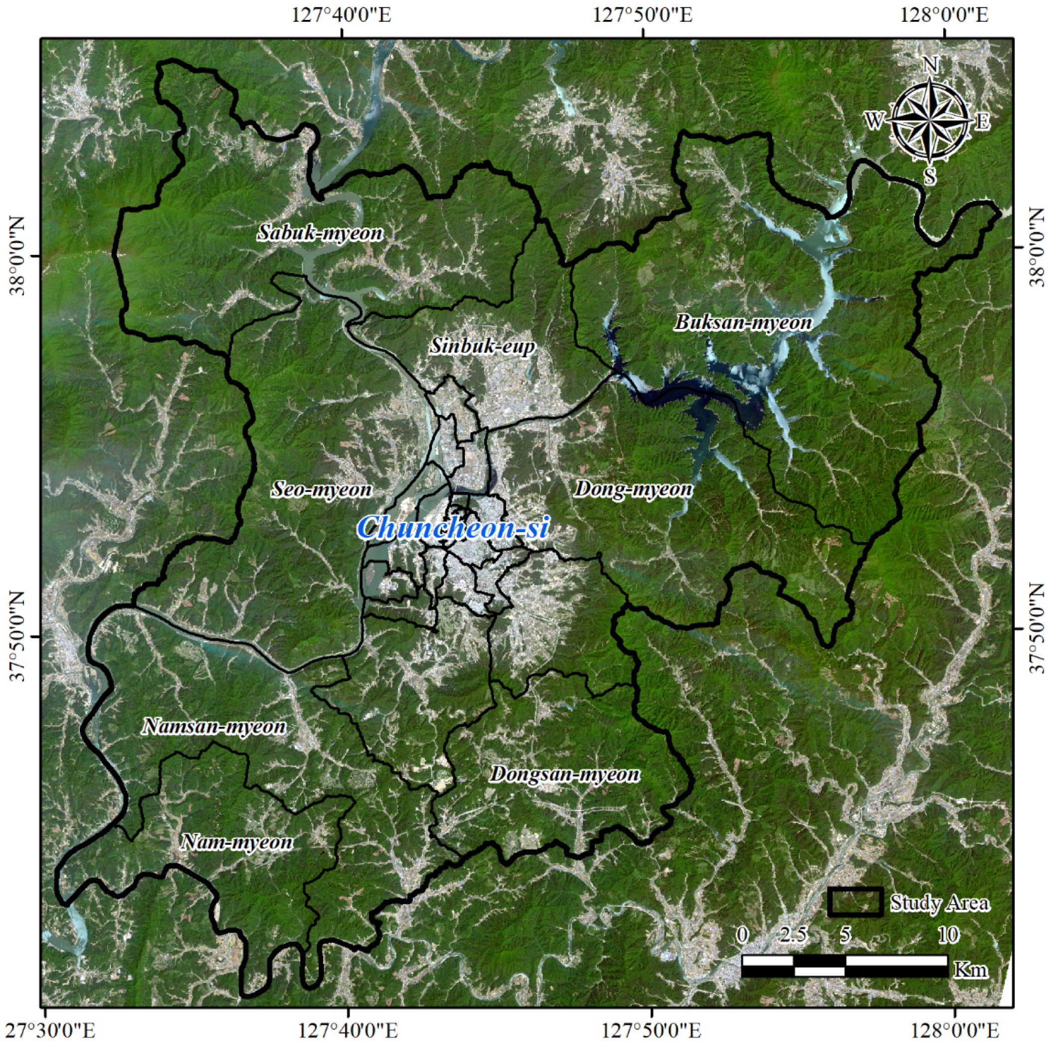
Figure 1. Study Area.
Remotesensing 16 02623 g001
Figure 2. Research method for land cover classification.
Remotesensing 16 02623 g002
Figure 3. Training dataset according to land cover categories.
Remotesensing 16 02623 g003
Figure 4. Architecture of the baseline deep learning model. The diagram illustrates the U-Net structure with encoder (left) and decoder (right) paths. Blue arrows indicate convolutional operations, grey arrows represent copy and crop operations, red arrows show max pooling, and green arrows indicate up-convolutions [26].
Remotesensing 16 02623 g004
Figure 5. Land cover maps produced according to datasets and deep learning models.
Remotesensing 16 02623 g005
Figure 6. Accuracy distribution of deep learning-based land cover map by categories.
Remotesensing 16 02623 g006
Figure 7. Examples of accuracy improvement in deep learning models for land cover classification: (1) Forestry-managed land, (2) Grassland, (3) Other land, and (4) Cropland.
Remotesensing 16 02623 g007
Table 1. Datasets for land cover classification using deep learning models (Unit: Count).
Training DataValidation DataTest DataDeep Learning Dataset
113476162Dataset A: R, G, B, RE, NIR
Dataset B: R, G, B, RE, NIR, GLCM
Dataset C: R, G, B, RE, NIR, Slope
Dataset D: R, G, B, RE, NIR, GLCM, Slope
Table 2. Confusion matrix of deep learning-based land cover classification.
CategoryModel ClassificationTotal
PositiveNegative
Label image
(True value)
PositiveTP (true positive)FN (false negative)TP + FN
NegativeFP (false positive)TN (true negative)FP + TN
TotalTP + FPFN + TNTP + FN + FP + TN
Table 3. Spectral characteristics of training data for land cover classification.
CategorySurface ReflectanceGLCMSlope
RedNIRCorrelationEntropyHomogeneity
Forest260 ± 1273337 ± 659−0.05 ± 0.317.83 ± 0.050.04 ± 0.0227.2 ± 10.9
Cropland1101 ± 5072547 ± 748−0.03 ± 0.347.80 ± 0.090.05 ± 0.034.8 ± 5.0
Grassland690 ± 4353186 ± 761−0.07 ± 0.347.82 ± 0.070.04 ± 0.0211.9 ± 10.1
Wetland459 ± 288821 ± 921−0.01 ± 0.307.53 ± 0.590.08 ± 0.091.3 ± 5.3
Settlement1369 ± 6642632 ± 651−0.06 ± 0.317.81 ± 0.080.04 ± 0.027.4 ± 8.3
Other land1690 ± 9352747 ± 9100.02 ± 0.377.77 ± 0.180.05 ± 0.0417.0 ± 16.2
Forestry-managed land640 ± 3663083 ± 8230.01 ± 0.357.82 ± 0.060.04 ± 0.0225.6 ± 10.0
Table 4. Results of training and validation of the deep learning model.
Deep Learning ModelDatasetTraining ResultsValidation ResultsTraining Time (min)
AccuracyLossAccuracyLoss
Model AA92.6 ± 0.70.231 ± 0.03082.5 ± 0.50.539 ± 0.019124.3 ± 4.0
B91.9 ± 1.40.250 ± 0.04381.7 ± 0.90.522 ± 0.023135.5 ± 2.6
C91.3 ± 1.10.302 ± 0.05480.9 ± 1.20.545 ± 0.022129.7 ± 3.5
D91.2 ± 0.80.270 ± 0.02580.9 ± 0.60.552 ± 0.011139.2 ± 3.9
Model BA85.7 ± 0.40.821 ± 0.00585.4 ± 0.30.829 ± 0.004124.3 ± 0.7
B85.6 ± 0.30.822 ± 0.00485.3 ± 0.30.830 ± 0.004135.3 ± 0.8
C86.2 ± 0.30.815 ± 0.00486.0 ± 0.30.823 ± 0.003129.0 ± 4.0
D86.2 ± 0.20.814 ± 0.00386.1 ± 0.30.821 ± 0.003139.8 ± 3.7
The average values of models trained with 10 repetitions at 1000 epochs.
Table 5. Evaluation of land cover map accuracy according to datasets and deep learning models.
DatasetModel AModel B
Overall Accuracy (%)KappaOverall Accuracy (%)Kappa
Dataset A88.1 ± 0.30.71 ± 0.0189.8 ± 0.30.77 ± 0.01
Dataset B86.5 ± 3.30.65 ± 0.0589.7 ± 0.30.76 ± 0.01
Dataset C87.3 ± 3.30.68 ± 0.0590.1 ± 0.40.77 ± 0.01
Dataset D88.0 ± 0.60.71 ± 0.0190.0 ± 0.40.77 ± 0.01
The average values of models trained with 10 repetitions at 1000 epochs.
Disclaimer/Publisher’s Note: The statements, opinions and data contained in all publications are solely those of the individual author(s) and contributor(s) and not of MDPI and/or the editor(s). MDPI and/or the editor(s) disclaim responsibility for any injury to people or property resulting from any ideas, methods, instructions or products referred to in the content.