Abstract
Sea ice plays a critical role in the Earth’s climate system, and its variations affect ecosystem stability. This study introduces a novel method for detecting sea ice in the Arctic Ocean using bidirectional radar reflections from the Global Navigation Satellite System (GNSS). Utilizing delay-Doppler maps (DDM) from the UK TechDemoSat-1 (TDS-1) satellite mission and surface data from the U.S. National Oceanic and Atmospheric Administration (NOAA), we employ the local linear embedding (LLE) algorithm for feature extraction. This approach notably reduces training costs and enhances real-time performance, while maintaining a high accuracy and robust noise immunity level. Focusing on the region above 70° north latitude throughout 2018, we aimed to distinguish between sea ice and seawater. The extracted DDM features via LLE are input into a support vector machine (SVM) for classification. The results indicate that our method achieves an accuracy of over 99% for selected low-noise data and a monthly average accuracy of 92.74% for data containing noise, while the CNN method has a monthly average accuracy of only 77.31% for noisy data. A comparative analysis between the LLE-SVM approach and the convolutional neural network (CNN) method demonstrated the superior anti-interference capabilities of the former. Additionally, the impact of the sea ice melting period on detection accuracy was analyzed.
1. Introduction
Sea ice is an important foundation of Earth’s ecology. Ninety percent of the world’s total ice and snow are in the polar circle, which is the world’s largest freshwater resource, with 78% of Earth’s freshwater reserves. In addition to being the largest freshwater reservoir, ice and snow in the polar region play important roles in regulating global temperature, global heat balance, and water balance [1]. The existence of sea ice and its variable physical states influence human activities [2]. Due to climate change, the lowlands, islands, and coastal areas of the world are at risk of being submerged. Coastlines have been affected and receding has been indicated. The ecological environment in coastal areas will be destroyed and coastal species will become extinct. Human activities may be restricted, for example, due to hindered economic development and restricted offshore fishing. The sea ice conditions each year are different, which means that sea ice test reports of previous years do not represent the true conditions of the current year. Obtaining information on global climate change, enabling human activities in the ocean, and adjusting coastal economic policies over time are important [3]. Sea ice detection can respond to these requirements, which reflects its practical significance. Because of the limitations of time and technology, field surveys are a common method for sea ice detection during its initial stages. With technological innovations, field surveys have been replaced by other technologies, such as passive microwave sensors [3], scatterometers [4,5,6], radar altimeters [7,8], and synthetic aperture radar (SAR) [9,10]. However, these technologies cannot meet all current needs. Passive microwave sensors can only be used in experiments with small areas and over short periods. Scatterometers rely on the stability of the signal and are easily affected by noise and other signals. Radar altimeter data take a long time to collect and cannot reflect sea ice conditions in real time. SAR relies on the hardware performance of satellites, and its data cannot be used in forecasting.
Global Navigation Satellite System-Reflectometry (GNSS-R) can solve some of these limitations: it is suitable for large-scale areas, has stable signals, and can collect large amounts of freely available real-time data. Hall and Cordey first proposed the concept of GNSS-R technology in 1988 [11]. GNSS-R technology uses GNSS signals to remotely sense the ocean’s surface, relying mainly on multipath interference effects [12,13]. At present, the specific applications of GNSS-R technology are related to the determination of the water level of the ocean [14], oil spill detection [15], the measurement of wind speed [16,17,18], sea ice thickness retrieval [19,20], soil moisture retrieval [21,22], snow depth detection [23], target detection [24,25], disaster warning [26], and surface water fraction retrieval [27]. With the development of sea ice detection applications, the main scientific research results have been related to sea ice concentration, classification, boundary detection, and thickness.
Many studies are based on delay-Doppler map (DDM) data for GNSS-R spaceborne sea ice detection. Traditional methods have made significant contributions to this field. In 2016, Yan and Huang [28] pioneered a novel approach for sea ice detection utilizing the TDS-1 dataset, introducing a suite of DDM observation metrics. This innovative method leveraged metrics such as pixel number (PN), power summation (PS), geometric center (GC) distance, center-of-mass (CM) distance, and CM taxicab distance to enhance the detection process. Zhu et al. [29] employed the image difference method on adjacent DDMs from TDS-1 to classify sea ice into four transition types: sea ice–sea water, sea ice–sea ice, sea water–sea water, and sea water–sea ice, achieving an accuracy rate of 96%. However, this approach depends on the stability of the output data, which limits its effectiveness for real-time processing. Rodriguez-Alvarez et al. [30] introduced the CART algorithm in 2019 for the multistep classification of sea ice types using DDM observables as inputs, with accuracies of 94% for multi-year ice, 54.5% for first-year ice, and 69.7% for young ice. Zhu et al. [31] proposed a sea ice detection method using a Doppler propagation analysis of spatial GNSS-R data to classify sea ice and seawater, which achieved an accuracy of 98.22% in the northern hemisphere and 96.65% in the southern hemisphere. In recent years, machine learning techniques have emerged as powerful tools for analyzing DDM data. Yan et al. [32] were the first to introduce machine learning algorithms to process DDMs from TDS-1, utilizing a neural network (NN) for sea ice and seawater classification as well as sea ice concentration estimations, with an accuracy of 93%. Following this, Yan and Huang [33] employed a convolutional neural network (CNN) for both sea ice detection and sea ice concentration retrieval, achieving a higher accuracy of 96%. These advancements highlight the potential of machine learning methods to improve classification accuracy and processing efficiency. Additionally, Hu et al. [34] applied the LDA method for sea ice detection, addressing issues related to the sea ice melting period and classifying DDMs based on the signal-to-noise ratio. They found that as the SNR decreases, the noise’s effects become more significant, leading to a notable decrease in detection accuracy. Despite these advancements, current machine learning methods still face challenges, including the need for large datasets and complex algorithms. This study aims to build on the strengths of existing methods and address their limitations to further enhance sea ice detection accuracy and real-time performance.
Although the CNN method has demonstrated a high accuracy in sea ice detection, it inevitably requires extensive preprocessing and faces the drawback of dimensionality, both of which significantly reduce its real-time performance. Specifically, the dimensionality of the DDM inputs used for training increases, leading to high training costs that limit its real-time detection capabilities. Moreover, without preprocessing steps such as noise floor adjustment or normalization [35], the accuracy of sea ice detection can be severely compromised. Sea ice and seawater DDMs are particularly susceptible to noise interference, resulting in less distinct features.
Dimension reduction can alleviate dimensionality and other undesirable properties of high-dimensional spaces as well as significantly reduce model complexity and training costs. In this paper, we propose to process DDMs from TDS-1 for sea ice detection with a local linear embedding (LLE) algorithm. A key advantage of LLE is its ability to preserve local geometric information about the data. This means that it can capture the local structural properties of the data, not just the global distributional properties. Unlike traditional linear dimensionality reduction methods (e.g., PCA), LLE can deal with non-linear relationships in data. When data present a nonlinear distribution in a high-dimensional space, LLE is better able to maintain the essential information of these nonlinear structures. LLE reduces the effect of noise by linear embedding in the local range, which makes LLE robust to noise and outliers in the data compared to other methods.
We propose to extract DDM features using the LLE dimensionality reduction algorithm and classify sea ice and seawater with an SVM. Our study focuses on the region above 70°N, where large areas of sea ice and seawater were present throughout 2018, providing diverse types of DDMs for detection. We use the National Oceanic and Atmospheric Administration’s (NOAA) sea ice type products as the ground truth and compare them to the sea ice detection results from the TDS-1 radar reflection data. Evaluating the performance of the LLE-SVM model with a selected dataset, we find that the LLE method is fast to train and achieves a high accuracy, enhancing real-time sea ice detection. Additionally, tests conducted with an unselected dataset demonstrate that LLE can tolerate noisy data, showing a better anti-interference performance. Finally, the effect of the sea ice’s melting period on sea ice detection is analyzed concerning the problem of the decrease in accuracy during its melting period.
2. Datasets and Methods
2.1. Adopted Datasets
The TDS-1 is a satellite platform designed as an in-orbit facility, carrying eight payloads, with the Space GNSS Receiver-Remote Sensing Instrument (SGR-ReSI) being the primary one. The main objective of TDS-1 is to demonstrate the technology and science required for GNSS reflectometry through the operation and collection of data over the ocean. The TDS-1 data used in this study are freely available on the Measurement of Earth Reflected Radio Navigation Signals by Satellite (MERRByS) website (http://merrbys.co.uk (accessed on 5 January 2023)), where the link to the mission data FTP site is accessible under data access/downloads (ftp://ftp.merrbys.co.uk (accessed on 5 January 2023)) after user registration.
Sea ice is primarily concentrated in high-latitude areas, so DDM data from regions above 70°N latitude were selected for the experiment. As shown in Table 1, the experimental data are divided into two parts: selected DDM and unselected DDM. The selected DDM has a high signal-to-noise ratio, and the sea ice and seawater features are clear. The unselected DDM contains noise and other interfering factors, and the features are blurred. In addition to the 7000 DDMs selected from February used as the training dataset, 16,537 DDMs were used to test the LLE-SVM-based model, and 563,034 DDMs were used to test the robustness of the LLE-SVM. The main reason for choosing the February data as the training set is that the feature performance of DDMs in February is usually clearer and more stable. By rigorously selecting the samples with the most distinctive features in that month, we can ensure that the training set has high data quality and consistency, thus providing a good starting point for model learning. The characteristics of sea ice and seawater change over seasons and months. Therefore, to assess the ability of the model to generalize across different months and conditions, we chose data spanning multiple months as a test set.

Table 1.
DDM count for each month in 2018.
The National Oceanic and Atmospheric Administration (NOAA) database provides a wealth of monthly meteorological and surface type data, including monthly temperature, precipitation, and snowfall records, as well as information covering a wide range of surface types, such as land, coastline, rivers, lakes, sea ice, and seawater. These data are acquired based on a variety of advanced observation and measurement techniques, including satellite remote sensing, buoy monitoring, survey station records, and in situ observations from aircraft and ships, and are subjected to rigorous quality control and quality assurance processes to ensure the accuracy and reliability of the data. NOAA not only excels in data collection and processing but also collaborates closely with international organizations and scientific research institutes worldwide to share data and observations, ensuring global data consistency and accuracy. Consequently, NOAA data are considered highly reliable and accurate on a global scale. Using these data, we merged and matched the latitude and longitude information from the DDM dataset with NOAA’s land surface type data. Through this method, we were able to accurately identify the land–sea distribution in the DDM data, thereby eliminating data from land, rivers, and lakes and retaining only the DDM data associated with sea ice and seawater. This step is essential for ensuring the accuracy and effectiveness of sea ice detection. The NOAA data used in this study are available online at the NOAA website (https://noaadata.apps.nsidc.org/NOAA/, accessed on 5 January 2023).
2.2. Theory of GNSS-R Spaceborne Remote Sensing
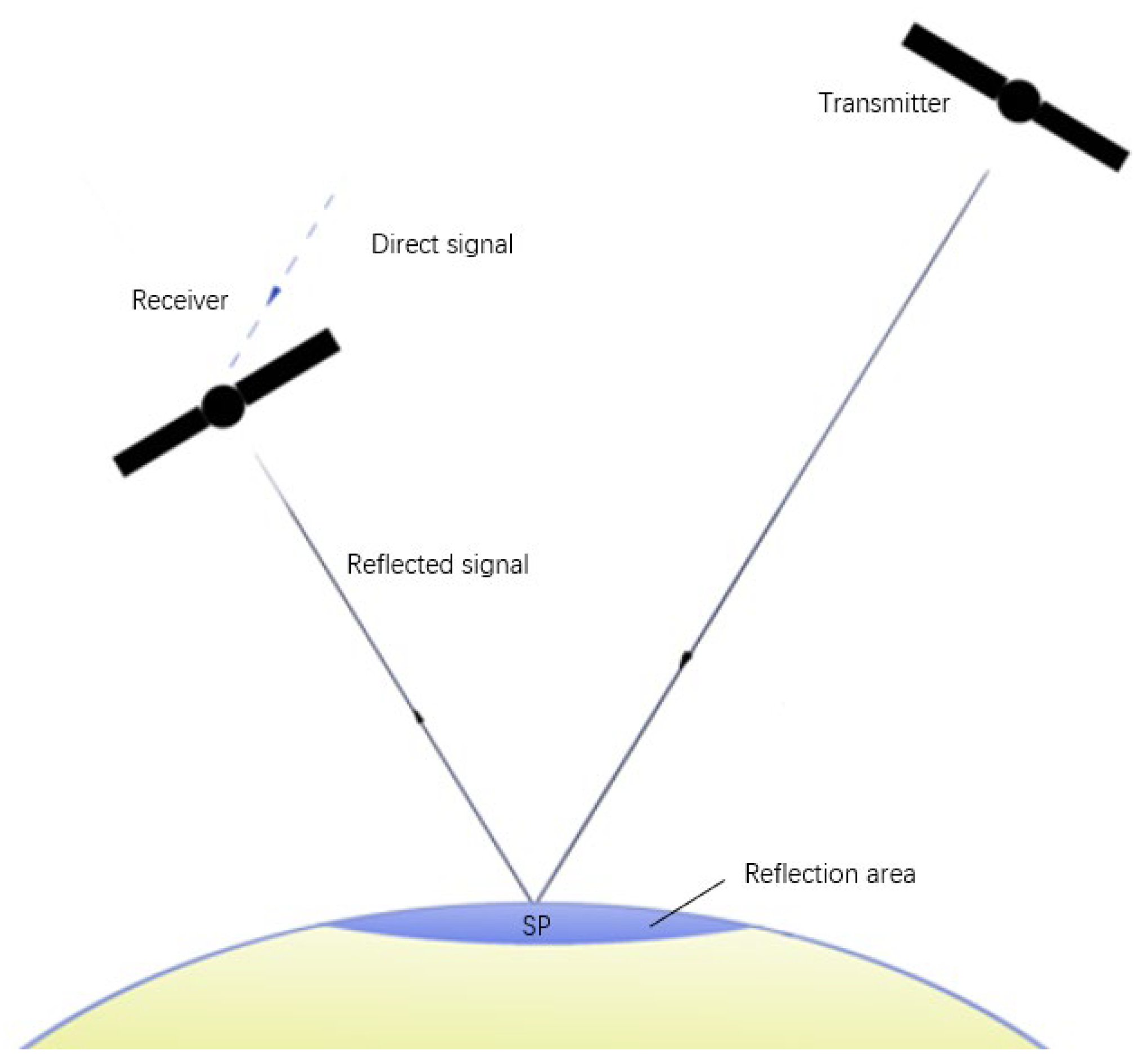
GNSS-R uses the reflected signal of the GNSS to sense the surface of the Earth, including features such as sea ice and seawater. The scattering reference model of the GNSS-R used for sea ice contains transmitters, receivers, and special points [36]. Signals emitted by the transmitters are reflected by the Earth’s surface and collected by the receivers. However, during transmission, the signals can be affected by factors such as radio frequency interference or instrument failure, leading to signal distortion. Therefore, the influence of interfering factors must be weakened in sea ice detection.
Figure 1 illustrates the GNSS-R remote sensing model. The solid line represents the reflected signal, which is reflected from the area around the specular point (SP) and is received by the receiver. The dashed line represents the direct signal received by the receiver. The blue area indicates the region where the signal from the transmitter is reflected, and SP is the center of reflection in the reflective zone. Since the transmitter is much higher than the receiver, the direct signal not reflected by the surface is parallel to the signal reflected by the surface. This delay can be described by the following equation:
where and are the coordinates of the transmitter and receiver in the global coordinate system. is the coordinate of a special point in the global coordinate system. is the speed of light, whose unit is .
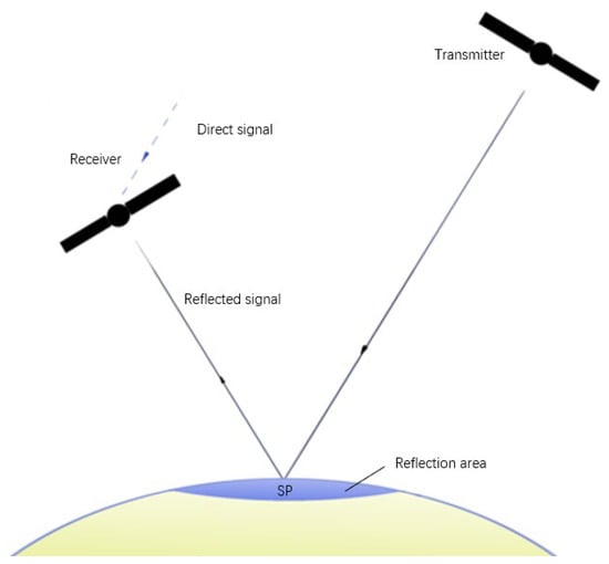
Figure 1.
Illustration of spaceborne remote sensing.
2.3. DDMs and IDWs
DDMs describe the power distribution in the reflective region at the delay time and Doppler frequency. As pointed out by Marchan-Hernandez et al. [37], in the L-band, the semitransparent layer of sea ice is used to describe the ice-covered sea surface, which is bound by seawater under sea ice. When the thickness of the sea ice is lower than the penetration depth (in the L-band, the penetration depth in saline ice can be up to 2 m, but it is greater for freshwater ice [38]), the lowermost seawater will be used to dominate the scattering. The ice–water interface can be treated as a smooth surface, as indicated by Helm [14]. As a result, only the incoming signals spread around the SP can be reflected and received by the receiver, which can be denoted as the DDM. The power distribution of the reflected signal over 2D space of code delay offsets and Doppler shift [39] can be expressed as follows:
where and are the delay and Doppler bin size, is the coherent integration time, is the antenna radiation pattern, where is the surface pixels of the scattering area, is the distance from the transmitter to the scattering point, is the distance from the scattering point to the receiver, is known as Woodward’s ambiguity function (WAF) [40], and is the sea surface scattering coefficient. is used to select specific values of time delay and Doppler shift. Therefore, Equation (2) can be rewritten as follows:
where is a scattering power function related to the scattering surface, observation geometry, the transmitter and receiver antenna pattern, and the propagation factors [41].
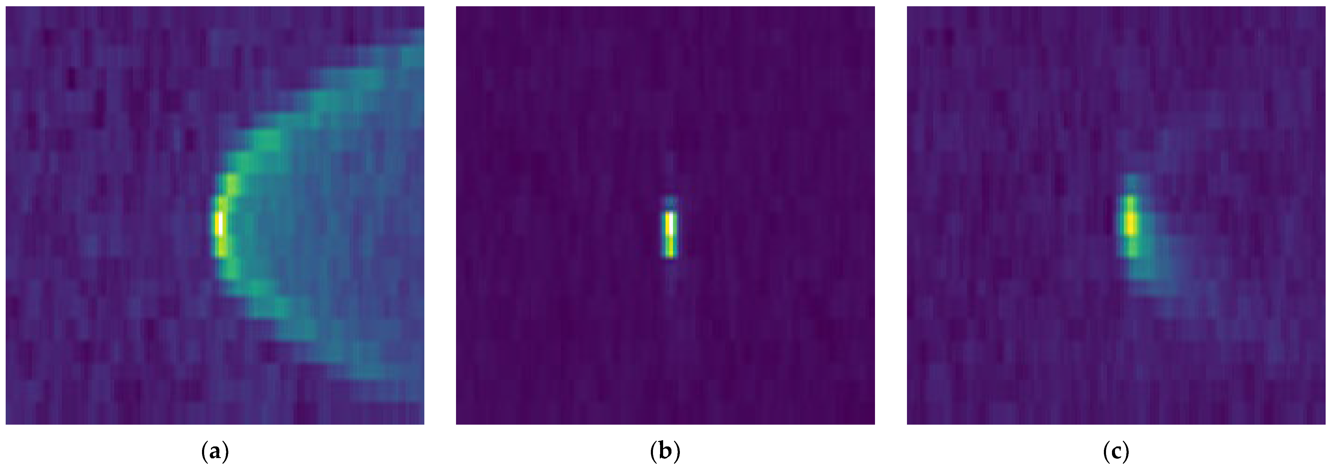
Typical DDMs are shown in Figure 2, where (a) is the DDM of sea ice, (b) is the DDM of seawater, and (c) is the DDM of ice–water mixture. The power of the sea ice DDM is concentrated in the center region, and that of the seawater DDM is in the shape of a horseshoe. However, the numerous features in the DDMs interact with each other. Therefore, sea ice detection cannot achieve the desired results without sufficient preprocessing. Sea ice detection is limited by the high-dimensional nature of the DDM; therefore, dimensionality reduction can weaken the influence of high dimensions.
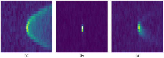
Figure 2.
DDMs collected by TDS-1: (a) Seawater DDM; (b) Sea ice DDM; (c) Ice–water mixture DDM.
The Doppler integral is a recent method used to process DDMs for sea ice detection. The output of the Doppler integral is the integral delay waveform (IDW), which describes the power of scattered signals as a function of the time delay. IDW was proposed by [31] and is written as follows:
where is the time delay value, is the Doppler shift frequency, and is the vector from the specular reflection point to the scattering point.
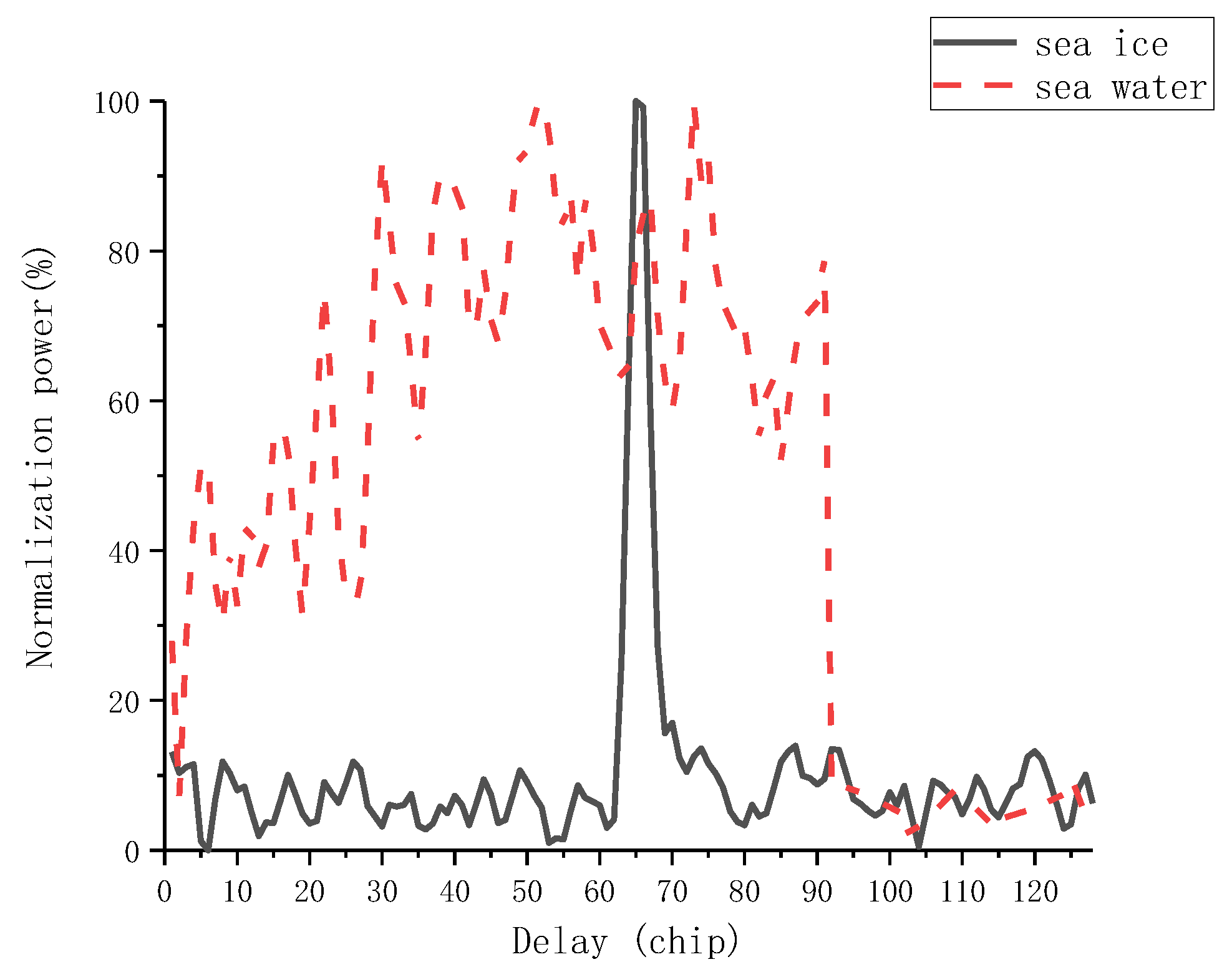
In Figure 3, the red line indicates the IDW of seawater, the black line indicates the IDW of sea ice, the horizontal axis indicates the coherent integration time, and the vertical axis indicates the power after Doppler integration. The figure clearly shows the difference between the IDWs of sea ice and seawater, in which the IDW of sea ice has only one peak, while the IDW of seawater has multiple peaks.
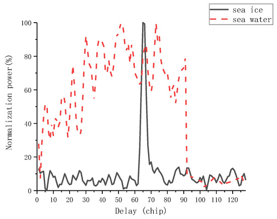
Figure 3.
IDWs of typical DDMs.
2.4. Locally Linear Embedding Algorithm
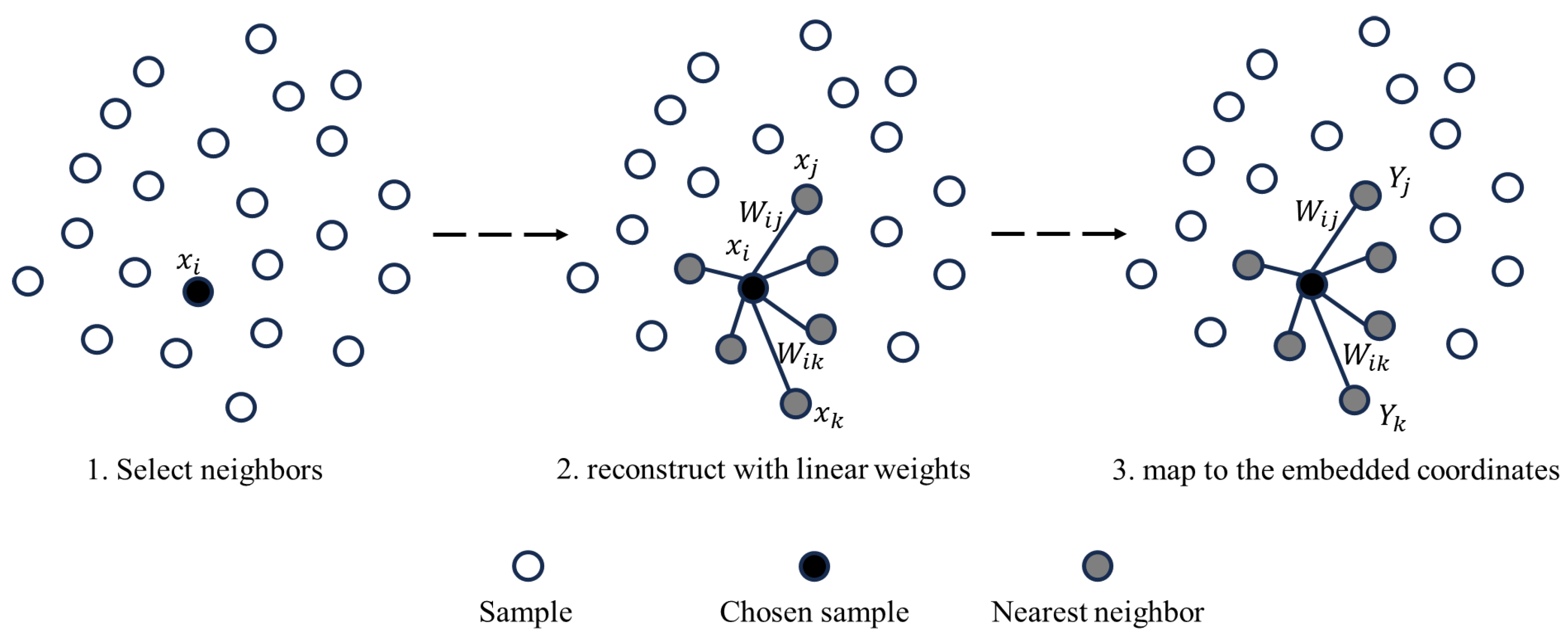
The LLE algorithm is a dimensionality reduction method [42]. The LLE attempts to preserve only the local structural graphical representation of the data points, which weakens the impact of too many features in the DDM. In LLE, the local properties of the data manifold are constructed by expressing high-dimensional data points as linear combinations of their immediate neighbors. This approach reduces the amount of data and extracts relevant features of sea ice and seawater, preserving the reconstruction weights in the IDW and ensuring the effectiveness of the extracted features for sea ice detection. Owing to the dimensionality reduction effect of LLE, the amount of data is reduced, which improves the efficiency of LLE-based sea ice detection and reduces the training cost. Overall, LLE can improve the anti-interference and real-time performance of sea ice detection while obtaining accurate sea ice detection results. As shown in Figure 4, the design of the LLE algorithm is divided into three steps.
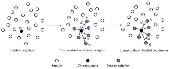
Figure 4.
Steps of LLE.
Step 1: Select neighbors. To determine the chosen neighbors, the number of chosen nearest neighbors is determined as seven, which is determined by a comparative experiment.
Step 2: Reconstruct linear weights. After the number of the chosen nearest neighbors is determined, the linear weights between the sample and its k-nearest neighbors should be constructed, whose dimensionality is 1 × 128. The main characteristic of the LLE is that the processed low-dimensional data can maintain the original topological relationship. The above relationship was determined using the k-nearest neighbor (KNN) method [43]. Specifically, it calculates the weight coefficient in the linear relationship between a sample and its k-nearest neighbor. The above question is a regression question; therefore, the mean square error can be used as the loss function. The loss function can be expressed as follows:
where and are the -th n-dimensional sample and the -th n-dimensional nearest neighbor. is the number of the sample. is the weight coefficient, which represents the linear relationship between and its -th nearest neighbor samples. satisfies the following functions:
where , is a one-dimensional matrix consisting of ones, and can be combined using Lagrangian multiplication [44], which is one optimization goal. can be described as follows:
where is the correlation coefficient of Lagrangian multiplication. The of high-dimensional data could be obtained by taking the derivative of in Function (7).
Step 3: Map to the embedded coordinates. After the linear weights are constructed, they are used to reduce the dimensionality of the IDW. Linear weights are used as the input, and low-dimensional data are used as the output.
While reducing the high-dimensional data by LLE, of high-dimensional data in Function (7) should remain unchanged. The n-dimensional data are . are low-dimensional data and represent the extracted features of IDW, whose dimensionality is . When the variance loss function, , is the smallest, the linear relationship is not changed. can be expressed as follows:
where and are the -th d-dimensional data and its -th d-dimensional nearest neighbor. and is the trace function. The restrictions of can be expressed as follows:
Function (11) can be combined into using Lagrangian multiplication, which is one optimization goal. can be described by the following:
where is a matrix composed of eigenvectors corresponding to the 2nd to th smallest eigenvalues of the matrix . After taking the derivative of , the smallest d-dimensional dataset can be obtained.
2.5. Support Vector Machine (SVM)
Support vector machine (SVM) is a two-class mode [45] used to learn extracted IDW features for sea ice detection. SVMs can solve nonlinear classification problems [46] and perform well in classification tasks. The task of the SVM is to achieve a hyperplane for classifying the types of IDWs based on their extracted features. The hyperplane can be expressed as follows:
where is normal vector determining the direction of the hyperplane. The number of eigenvalues is described as d. is the sample for training the SVM and provides the true data. is the displacement term determining the distance between the hyperplane and the origin data.
The settings for the SVM were as follows. A Gaussian kernel was chosen as the kernel of the SVM. The maximum number of iterations is set as −1, which means that the iteration is unlimited. The penalty slack variable is set to 1. After the establishment of the SVM-based model, the processed data from the IDW by LLE are input into the SVM and categorized into sea ice or seawater.
2.6. Process of GNSS-R Sea Ice Detection
The sea ice detection algorithm process includes three steps: data processing, model training, and model testing. The specific steps are as follows.
- Pre-process the DDM data collected by TDS-1:
Signal box screening. To filter out valid DDMs and reduce the effects of various factors, data are screened with a signal box. According to the TDS-1 manual, the data in NoiseBoxRow show how to distinguish the DDMs from the whole signal. When the parameter at that time is not zero, the DDM of that time has an entire signal.
Doppler integral. The Doppler integral of DDMs is used in the processing steps to reduce the amount of data processed in the experiment and the interference of DDMs’ features. The results of the Doppler integral were IDWs. IDWs can be obtained using Equation (4).
Normalize. To strengthen the characteristics of IDWs, they were normalized. The IDWs are normalized with respect to their real-time power as a percentage of the peak power. The percentage is determined as follows:
where is the real-time power in IDWs, and and are the minimum and the maximum in the IDWs.
- 2.
- Use the LLE algorithm for feature extraction, then take the extracted features as the input of SVM and the sea ice detection results as the output.
- 3.
- Determine the optimal parameters of the model and select the best model for sea ice detection.
3. Results and Analysis
LLE-based sea ice detection was tested in two different environments: an ideal environment (where the data are fully preprocessed and retain DDMs with high SNR values) and a noisy environment (where the data contain interfering factors such as noise). In the ideal environment, we evaluated the LLE-based sea ice detection model and examined the superiority of LLE in terms of its accuracy and real-time performance by comparing the performance of the LLE and CNN methods. In the noisy environment, we verified the anti-interference performance of the target method by comparing the accuracy of the LLE and CNN methods. In this study, we also analyzed the effect of temperature on sea ice detection.
3.1. Sea Ice Detection with Selected DDMs
In this paper, we first evaluate the performance of LLE-based sea ice detection in an ideal environment. The data of 7000 DDMs in 2018 are selected as the training set, and the data from March to December are tested as the test set. Table 2 gives the LLE-SVM method’s sea ice detection results for March–December 2018 in the ideal environment, and it can be seen that the accuracy of all of the test datasets is higher than 99%. A total of 16,537 IDW data points were tested, of which 16,492 DDMs were correctly classified with an accuracy of 99.725%.

Table 2.
Results of LLE-based sea ice detection with selected DDMs.
To demonstrate the superiority of LLE-based sea ice detection in terms of accuracy and real-time performance, we compared it with a CNN-based sea ice detection model. Due to the high training cost and long testing time for large datasets, a small dataset of 1000–5000 DDMs is selected for the experiments. Both methods were tested using the same dataset. The comparison mainly focuses on three aspects: accuracy, data volume, and processing time. The configuration of the experimental environment is presented in Table 3.

Table 3.
Experimental environment configuration.
Table 4 presents the sea ice detection results for datasets of different sizes. As can be seen from the increase in the number of DDMs, the accuracy of the CNN first increased and then decreased, with an average accuracy of 86.2608%. This is due to the limited random-access memory (RAM) storage space, and the model is not able to make full use of all the available data as it is not able to load all the data into the system’s memory for training at the same time. CNNs require larger-scale data to fine-tune the model’s weights, but an excessive amount of data can cause the training time to grow exponentially. In contrast, the LLE-based model for sea ice detection avoids these issues and achieves an accuracy of 97.3079%, which is 11.047% higher than the average accuracy of the CNN-based model.

Table 4.
Comparison of CNN and LLE in terms of accuracy, data size, and real-time performance.
This study compared the sizes of the DDM data processed by the LLE and CNN methods. The data size for the CNN method reached the GB level, while the LLE method produced data sizes at the KB level. This significant difference in data size directly influenced the feasibility of conducting experiments in the study’s environment. Specifically, the CNN method’s data size was 50,103 times larger than that of the LLE method, contributing to the high training cost and poor real-time performance of the CNN.
To highlight the superiority of LLE in real time, the CNN and LLE methods were compared at the time level. The time includes the training and processing times. The training time of the CNN was 3500 s, and that of method was 51 s, making the CNN’s training time 841 times longer than that of the LLE-SVM. For processing 1000 DDMs, the CNN’s processing time was 13.82 times that of LLE. As the number of DDMs increased, the processing time disparity grew: for 2000 DDMs, the CNN took 17.44 times longer; for 3000 DDMs, it took 27.92 times longer; for 4000 DDMs, it took 29.86 times longer; and for 5000 DDMs, it took 33.79 times longer than LLE. This increasing gap highlights the LLE method’s superior real-time performance and feasibility compared to the CNN.
3.2. Sea Ice Detection with Unselected DDMs
To test the anti-interference performance of LLE-based sea ice detection, we used the noise-containing DDM collected by TDS-1, analyzed the anti-noise performance of LLE-SVM, and compared it with the accuracy of the CNN method; the experimental details are listed in Table 5.

Table 5.
Sea ice detection results with unselected DDMs.
Table 5 shows the results of sea ice detection with noisy data. The data were selected from February to December 2018, with a total of 563,034 IDWs. The results of sea ice detection show that the average accuracy of the LLE-SVM method is 92.74%, the average accuracy of the SVM is 79.69, and the average accuracy of the CNN is 77.31%. The accuracy trend of the SVM is similar to that of LLE-SVM, but the accuracy and stability of LLE-SVM are better than those of the SVM. The results show that the downscaled features with LLE are favorable for SVM-based sea ice detection. As shown in Figure 5, the accuracy of the CNN decreases substantially from June to September, while LLE-SVM is still stable but also shows a decreasing trend. For the unselected DMM, the sea ice and seawater DDM features are blurred due to noise and other disturbing factors, which affect the accuracy of the CNN. The LLE extraction of IDW features seems to weaken this effect. As can be seen from the table, the accuracy of the sea ice detection method decreases severely from June to September. This is because the sea ice melts during these months due to high temperatures, and the ice–water mixture during the melting period interferes with the sea ice detection. The effect of sea ice melting periods on sea ice detection is detailed in Section 3.3.
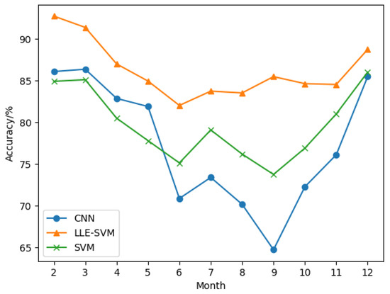
Figure 5.
The accuracy of sea ice detection with unselected DDMs.
Since DDM data from sea ice and seawater are often interfered with by various noise sources in practical applications, we purposely chose datasets without strict quality control for our experiments. Such a design helps reveal the model’s more general performance in real environments but leads to a decrease in sea ice detection accuracy.
To visually analyze the results of the LLE-SVM method for sea ice detection, NOAA data were used in this study to plot the real surface data and the predicted results for comparison, as shown in Figure 6. The predictions in Figure 6a–c show that the predictions for sea ice and seawater are correct when compared to the NOAA data. The boundaries of sea ice and seawater were consistent with those provided by the NOAA. These plots show that the LLE-SVM method also has a good classification performance for noisy DDMs. Figure 6d,e show the results of the sea ice soundings for the entire month. These plots show that the LLE-based sea ice detection method is robust and can correctly classify noisy data.
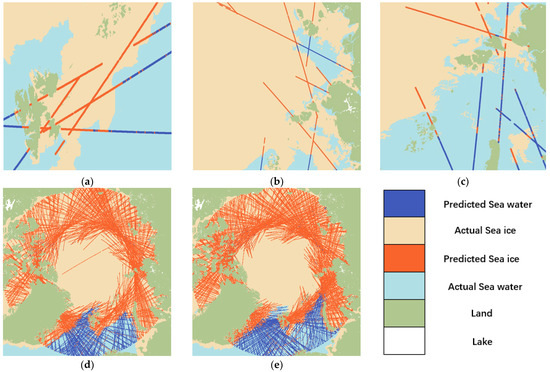
Figure 6.
The sea ice detection results of some days or months: (a) the results of sea ice detection on 18 February 2018, (b) the results of sea ice detection on 1 July 2018, (c) the results of sea ice detection in 2 August 2018, (d) the results of sea ice detection in February 2018, and (e) the results of sea ice detection in April 2018.
3.3. Analysis of Sea Ice Detection during Sea Ice Melting
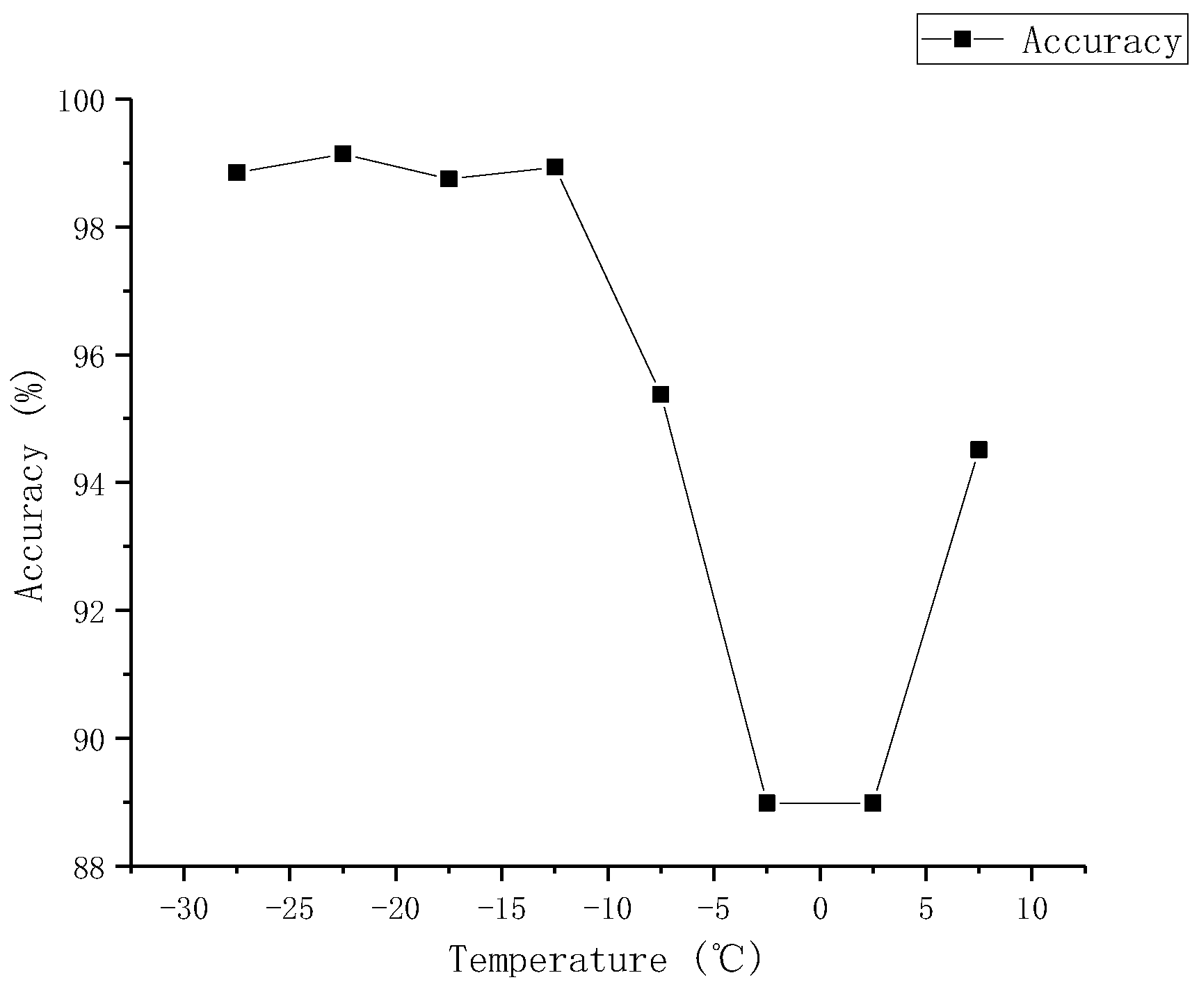
As there was a significant downward trend in the accuracy of sea ice detection in May, June, and July, we analyzed the relationship between the temperature and sea ice detection results. The temperatures, obtained from the monthly temperature range in 2018, were divided into 5 °C intervals. In February, temperatures were below −20 °C, and they gradually increased over time, with temperatures above 0 °C indicating the melting of sea ice. Figure 7 shows that at temperatures below −10 °C, the sea ice detection results are excellent, with an accuracy of over 95%, and very stable. However, as temperatures approach 0 °C, the accuracy of sea ice detection decreases, with an average accuracy of 88.98%. The presence of an ice–water mixture affects the characteristics of LLE at temperatures near 0 °C. As shown in Figure 2c, the DDM of the ice–water mixture is similar to that of sea ice and seawater, and the blurring of the characteristics leads to misclassifications. This result indicates that temperature is an important parameter affecting sea ice detection, and the presence of ice–water mixtures limits the accuracy of sea ice detection.

Figure 7.
The effect of temperature on sea ice detection.
Based on the LLE sea ice detection model, this paper analyses sea ice melting and compares the sea ice detection results collected at the beginning, middle, and end of each month, as shown in Figure 8. Figure 8a presents the melting conditions of the sea ice in June 2018. The area focused on in the black box is used to observe sea ice melting. Figure 8b1,b2 were adopted to show the sea ice extent in 2 June and 29 June in the chosen area. There was significant sea ice melting when comparing these two figures. To further illustrate the sea ice melting conditions, the sea ice melting statuses of 4, 18 and 29 June are shown in Figure 8c1–c3. The sea ice melting area was larger than that at the beginning of June 2018. Figure 8d1–d3 display the LLE-based sea ice detection results for the selected region, in which the transition from orange to blue dots represents the sea ice melting progression. This observation demonstrates that the LLE-based sea ice detection method effectively reflects the sea ice melting process.
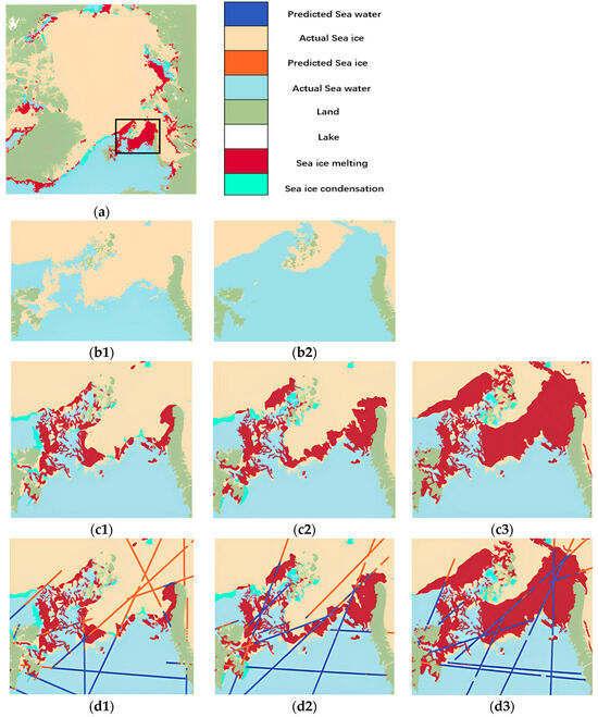
Figure 8.
Sea ice melt extent and LLE-SVM sea ice detections at the beginning, middle, and end of June 2018: (a) Sea ice melt in June 2018; (b1,b2) Sea ice extent on 2 June and 29 June; (c1–c3) Sea ice melt extent on 4, 18, and 29 June; (d1–d3) LLE-SVM sea ice detection on 4, 18, and 29 June.
Although the method proposed in this paper has made some progress in sea ice detection, it still has some limitations. The method performs poorly in terms of accuracy during the sea ice melting period. In addition, this method is highly dependent on a single data source and fails to take full advantage of other data sources that may enhance the performance of the model. To overcome these limitations, future research could consider introducing additional data sources, such as high-resolution satellite images, meteorological data, or oceanographic observations, to improve the generalization ability and robustness of the model. In addition, to address the impact of the ablation period on sea ice detection results, subsequent research will focus on DDMs of ice–water mixtures to further improve the sea ice detection accuracy during the ablation period. The ultimate goal is to find a sea ice detection method that can solve the problem of accuracy degradation during the ablation period and also meet the real-time requirements.
4. Conclusions
The experiment first examines the accuracy, stability, and real-time performance of the LLE model. The results show that the accuracy of the LLE-based sea ice detection method reaches 99.5149%, with a low training cost and real-time performance. For the unselected DDM data, the accuracy of the LLE-based model is 92.74%, and the comparison between the LLE method and the CNN method highlights the superiority of the LLE-based sea ice detection method in terms of anti-interference performance. In addition, the effect of temperature on the sea ice detection results is also analyzed in this study. The accuracy of sea ice detection decreases when an ice–water mixture occurs at a temperature of about 0 °C. In the future, the generalization ability and robustness of the model can be enhanced by introducing more data sources, such as high-resolution satellite images, meteorological data, or ocean observation data. In addition, to address the impact of the melting period on the sea ice detection results, subsequent research on DDMs of ice–water mixtures will be conducted to improve the accuracy of sea ice detection during melting periods.
Author Contributions
Conceptualization, X.H. and Z.J.; Methodology, X.H., Z.J. and Y.H.; Funding acquisition, Y.H. and W.L.; Projection administration, W.L., J.W. and Y.H.; Writing—original draft, X.H.; Writing—review and editing, Y.H., W.L., J.W., Q.Y., and X.H. All authors have read and agreed to the published version of the manuscript.
Funding
The research was funded by the National Natural Science Foundation of China under Grant 52071199.
Data Availability Statement
Spaceborne GNSS-R DDM data were collected from TechDemoSat-1. A large number of datasets from all regions of the world are available online (http://www.merrbys.co.uk (accessed on 5 January 2023)). The surface type data from the NOAA are available on the NOAA website (https://noaadata.apps.nsidc.org/NOAA/ (accessed on 5 January 2023)).
Acknowledgments
The authors additionally acknowledge the TDS-1 team for making the GNSS-R DDM data available, as well as the NOAA for providing the ground truth data for our comparative analysis.
Conflicts of Interest
The authors declare no conflicts of interest.
References
- Soukissian, T.; Karathanasi, F.; Axaopoulos, P.; Voukouvalas, E.; Kotroni, V. Offshore Wind Climate Analysis and Variabil-ity in the Mediterranean Sea. Int. J. Climatol. 2018, 38, 384–402. [Google Scholar] [CrossRef]
- Min, S.; Zhang, X.; Zwiers, F.W.; Agnew, T. Human Influence on Arctic Sea Ice Detectable from Early 1990s Onwards. Geophys. Res. Lett. 2008, 35, 2008GL035725. [Google Scholar] [CrossRef]
- Meier, W.N.; Stewart, J.S. Assessing Uncertainties in Sea Ice Extent Climate Indicators. Environ. Res. Lett. 2019, 14, 035005. [Google Scholar] [CrossRef]
- Belmonte Rivas, M.; Otosaka, I.; Stoffelen, A.; Verhoef, A. A Scatterometer Record of Sea Ice Extents and Backscatter: 1992–2016. Cryosphere 2018, 12, 2941–2953. [Google Scholar] [CrossRef]
- Zhang, Z.; Yu, Y.; Li, X.; Hui, F.; Cheng, X.; Chen, Z. Arctic Sea Ice Classification Using Microwave Scatterometer and Radiometer Data during 2002–2017. IEEE Trans. Geosci. Remote Sens. 2019, 57, 5319–5328. [Google Scholar] [CrossRef]
- Otosaka, I.; Belmonte Rivas, M.; Stoffelen, A. Bayesian Sea Ice Detection with the ERS Scatterometer and Sea Ice Backscatter Model at C-Band. IEEE Trans. Geosci. Remote Sens. 2018, 56, 2248–2254. [Google Scholar] [CrossRef]
- Laxon, S.; Peacock, N.; Smith, D. High Interannual Variability of Sea Ice Thickness in the Arctic Region. Nature 2003, 425, 947–950. [Google Scholar] [CrossRef] [PubMed]
- Rose, S.K.; Andersen, O.B.; Passaro, M.; Ludwigsen, C.A.; Schwatke, C. Arctic Ocean Sea Level Record from the Complete Radar Altimetry Era: 1991–2018. Remote Sens. 2019, 11, 1672. [Google Scholar] [CrossRef]
- Landy, J.C.; Tsamados, M.; Scharien, R.K. A Facet-Based Numerical Model for Simulating SAR Altimeter Echoes from Heterogeneous Sea Ice Surfaces. IEEE Trans. Geosci. Remote Sens. 2019, 57, 4164–4180. [Google Scholar] [CrossRef]
- Liu, H.; Guo, H.; Li, X.-M.; Zhang, L. An Approach to Discrimination of Sea Ice from Open Water Using SAR Data. In Proceedings of the 2016 IEEE International Geoscience and Remote Sensing Symposium (IGARSS), Beijing, China, 10–15 July 2016; IEEE: Piscataway, NJ, USA, 2016; pp. 4865–4867. [Google Scholar]
- Bishop, T.N.; Bube, K.P.; Cutler, R.T.; Langan, R.T.; Love, P.L.; Resnick, J.R.; Shuey, R.T.; Spindler, D.A.; Wyld, H.W. Tomo-graphic Determination of Velocity and Depth in Laterally Varying Media. Geophysics 1985, 50, 903–923. [Google Scholar] [CrossRef]
- Zavorotny, V.U.; Voronovich, A.G. Scattering of GPS Signals from the Ocean with Wind Remote Sensing Application. IEEE Trans. Geosci. Remote Sens. 2000, 38, 951–964. [Google Scholar] [CrossRef]
- Garrison, J.L.; Katzberg, S.J. Detection of Ocean Reflected GPS Signals: Theory and Experiment. In Proceedings of the Proceedings IEEE SOUTHEASTCON’97.’Engineering the New Century’, Blacksburg, VA, USA, 12–14 April 1997; pp. 290–294. [Google Scholar]
- Helm, A. Ground-Based GPS Altimetry with the L1 OpenGPS Receiver Using Carrier Phase Delay Observations of Reflected GPS Signals. Ph.D. Thesis, GeoForschungsZentrum, Potsdam, Germany, 2008. Scientific Technical Report. [Google Scholar]
- Valencia, E.; Camps, A.; Rodriguez-Alvarez, N.; Park, H.; Ramos-Perez, I. Using GNSS-R Imaging of the Ocean Surface for Oil Slick Detection. IEEE J. Sel. Top. Appl. Earth Obs. Remote Sens. 2013, 6, 217–223. [Google Scholar] [CrossRef]
- Zhao, D.; Heidler, K.; Asgarimehr, M.; Arnold, C.; Xiao, T.; Wickert, J.; Zhu, X.X.; Mou, L. DDM-Former: Transformer Net-works for GNSS Reflectometry Global Ocean Wind Speed Estimation. Remote Sens. Environ. 2023, 294, 113629. [Google Scholar] [CrossRef]
- Guo, W.; Du, H.; Guo, C.; Southwell, B.J.; Cheong, J.W.; Dempster, A.G. Information Fusion for GNSS-R Wind Speed Retrieval Using Statistically Modified Convolutional Neural Network. Remote Sens. Environ. 2022, 272, 112934. [Google Scholar] [CrossRef]
- Asgarimehr, M.; Arnold, C.; Weigel, T.; Ruf, C.; Wickert, J. GNSS Reflectometry Global Ocean Wind Speed Using Deep Learning: Development and Assessment of CyGNSSnet. Remote Sens. Environ. 2022, 269, 112801. [Google Scholar] [CrossRef]
- Xie, Y.; Yan, Q. Stand-Alone Retrieval of Sea Ice Thickness from FY-3E GNOS-R Data. IEEE Geosci. Remote Sens. Lett. 2024, 21, 2000305. [Google Scholar] [CrossRef]
- Yan, Q.; Huang, W. Sea Ice Thickness Measurement Using Spaceborne GNSS-R: First Results with TechDemoSat-1 Data. IEEE J. Sel. Top. Appl. Earth Observ. Remote Sens. 2020, 13, 577–587. [Google Scholar] [CrossRef]
- Yan, Q.; Gong, S.; Jin, S.; Huang, W.; Zhang, C. Near Real-Time Soil Moisture in China Retrieved From CyGNSS Reflectivity. IEEE Geosci. Remote Sens. Lett. 2022, 19, 8004205. [Google Scholar] [CrossRef]
- Yan, Q.; Huang, W.; Jin, S.; Jia, Y. Pan-Tropical Soil Moisture Mapping Based on a Three-Layer Model from CYGNSS GNSS-R Data. Remote Sens. Environ. 2020, 247, 111944. [Google Scholar] [CrossRef]
- Yu, K.; Wang, S.; Li, Y.; Chang, X.; Li, J. Snow Depth Estimation with GNSS-R Dual Receiver Observation. Remote Sens. 2019, 11, 2056. [Google Scholar] [CrossRef]
- Southwell, B.J.; Cheong, J.W.; Dempster, A.G. A Matched Filter for Spaceborne GNSS-R Based Sea-Target Detection. IEEE Trans. Geosci. Remote Sens. 2020, 58, 5922–5931. [Google Scholar] [CrossRef]
- Di Simone, A.; Park, H.; Riccio, D.; Camps, A. Sea Target Detection Using Spaceborne GNSS-R Delay-Doppler Maps: Theo-ry and Experimental Proof of Concept Using TDS-1 Data. IEEE J. Sel. Top. Appl. Earth Obs. Remote Sens. 2017, 10, 4237–4255. [Google Scholar] [CrossRef]
- Yan, Q.; Huang, W. Tsunami Detection and Parameter Estimation from GNSS-R Delay-Doppler Map. IEEE J. Sel. Top. Appl. Earth Obs. Remote Sens. 2016, 9, 4650–4659. [Google Scholar] [CrossRef]
- Yan, Q.; Liu, S.; Chen, T.; Jin, S.; Xie, T.; Huang, W. Mapping Surface Water Fraction over the Pan-Tropical Region Using CYGNSS Data. IEEE Trans. Geosci. Remote Sens. 2024, 62, 5800914. [Google Scholar] [CrossRef]
- Yan, Q.; Huang, W. Spaceborne GNSS-R Sea Ice Detection Using Delay-Doppler Maps: First Results from the U.K. TechDemoSat-1 Mission. IEEE J. Sel. Top. Appl. Earth Obs. Remote Sens. 2016, 9, 4795–4801. [Google Scholar] [CrossRef]
- Zhu, Y.; Yu, K.; Zou, J.; Wickert, J. Sea Ice Detection Based on Differential Delay-Doppler Maps from UK TechDemoSat-1. Sensors 2017, 17, 1614. [Google Scholar] [CrossRef] [PubMed]
- Rodriguez-Alvarez, N.; Holt, B.; Jaruwatanadilok, S.; Podest, E.; Cavanaugh, K.C. An Arctic Sea Ice Multi-Step Classifica-tion Based on GNSS-R Data from the TDS-1 Mission. Remote Sens. Environ. 2019, 230, 111202. [Google Scholar] [CrossRef]
- Zhu, Y.; Tao, T.; Yu, K.; Li, Z.; Qu, X.; Ye, Z.; Geng, J.; Zou, J.; Semmling, M.; Wickert, J. Sensing Sea Ice Based on Doppler Spread Analysis of Spaceborne GNSS-R Data. IEEE J. Sel. Top. Appl. Earth Observ. Remote Sens. 2020, 13, 217–226. [Google Scholar] [CrossRef]
- Yan, Q.; Huang, W.; Moloney, C. Neural Networks Based Sea Ice Detection and Concentration Retrieval From GNSS-R Delay-Doppler Maps. IEEE J. Sel. Top. Appl. Earth Observ. Remote Sens. 2017, 10, 3789–3798. [Google Scholar] [CrossRef]
- Yan, Q.; Huang, W. Sea Ice Sensing From GNSS-R Data Using Convolutional Neural Networks. IEEE Geosci. Remote Sens. Lett. 2018, 15, 1510–1514. [Google Scholar] [CrossRef]
- Hu, Y.; Jiang, Z.; Liu, W.; Yuan, X.; Hu, Q.; Wickert, J. GNSS-R Sea Ice Detection Based on Linear Discriminant Analysis. IEEE Trans. Geosci. Remote Sens. 2023, 61, 5800812. [Google Scholar] [CrossRef]
- Rothe, I.; Susse, H.; Voss, K. The Method of Normalization to Determine Invariants. IEEE Trans. Pattern Anal. Mach. Intell. 1996, 18, 366–376. [Google Scholar] [CrossRef]
- Park, H.; Pascual, D.; Camps, A.; Martin, F.; Alonso-Arroyo, A.; Carreno-Luengo, H. Analysis of Spaceborne GNSS-R De-lay-Doppler Tracking. IEEE J. Sel. Top. Appl. Earth Obs. Remote Sens. 2014, 7, 1481–1492. [Google Scholar] [CrossRef]
- Marchan-Hernandez, J.F.; Camps, A.; Rodriguez-Alvarez, N.; Valencia, E.; Bosch-Lluis, X.; Ramos-Perez, I. An Efficient Algorithm to the Simulation of Delay–Doppler Maps of Reflected Global Navigation Satellite System Signals. IEEE Trans. Geosci. Remote Sens. 2009, 47, 2733–2740. [Google Scholar] [CrossRef]
- Clarizia, M.P.; Ruf, C.; Cipollini, P.; Zuffada, C. First Spaceborne Observation of Sea Surface Height Using GPS-Reflectometry. Geophys. Res. Lett. 2016, 43, 767–774. [Google Scholar] [CrossRef]
- Zhang, G.; Guo, J.; Yang, D.; Wang, F.; Gao, H. Sea Ice Edge Detection Using Spaceborne GNSS-R Signal. Geomat. Inf. Sci. Wuhan Univ. 2019, 44, 668–674. [Google Scholar]
- Eustice, D.; Baylis, C.; Marks, R.J. Woodward’s Ambiguity Function: From Foundations to Applications. In Proceedings of the 2015 Texas Symposium on Wireless and Microwave Circuits and Systems (WMCS), Waco, TX, USA, 23–24 April 2015; IEEE: Piscataway, NJ, USA, 2015; pp. 1–17. [Google Scholar]
- Foti, G.; Gommenginger, C.; Unwin, M.; Jales, P.; Tye, J.; Roselló, J. An Assessment of Non-Geophysical Effects in Space-borne GNSS Reflectometry Data from the UK TechDemoSat-1 Mission. IEEE J. Sel. Top. Appl. Earth Obs. Remote Sens. 2017, 10, 3418–3429. [Google Scholar] [CrossRef]
- Chojnacki, W.; Brooks, M.J. A Note on the Locally Linear Embedding Algorithm. Int. J. Patt. Recogn. Artif. Intell. 2009, 23, 1739–1752. [Google Scholar] [CrossRef]
- Zhang, H.; Berg, A.C.; Maire, M.; Malik, J. SVM-KNN: Discriminative Nearest Neighbor Classification for Visual Category Recognition. In Proceedings of the 2006 IEEE Computer Society Conference on Computer Vision and Pattern Recognition (CVPR’06), New York, NY, USA, 17–22 June 2006; IEEE: New York, NY, USA, 2006; Volume 2, pp. 2126–2136. [Google Scholar]
- Negre, C.; Plantard, T. Efficient Modular Arithmetic in Adapted Modular Number System Using Lagrange Representation. In Information Security and Privacy; Mu, Y., Susilo, W., Seberry, J., Eds.; Lecture Notes in Computer Science; Springer: Berlin/Heidelberg, Germany, 2008; Volume 5107, pp. 463–477. [Google Scholar]
- Pal, M.; Mather, P. Support Vector Machines for Classification in Remote Sensing. Int. J. Remote Sens. 2005, 26, 1007–1011. [Google Scholar] [CrossRef]
- Yan, Q.; Huang, W. Detecting Sea Ice from TechDemoSat-1 Data Using Support Vector Machines with Feature Selection. IEEE J. Sel. Top. Appl. Earth Observ. Remote Sens. 2019, 12, 1409–1416. [Google Scholar] [CrossRef]
Disclaimer/Publisher’s Note: The statements, opinions and data contained in all publications are solely those of the individual author(s) and contributor(s) and not of MDPI and/or the editor(s). MDPI and/or the editor(s) disclaim responsibility for any injury to people or property resulting from any ideas, methods, instructions or products referred to in the content. |
© 2024 by the authors. Licensee MDPI, Basel, Switzerland. This article is an open access article distributed under the terms and conditions of the Creative Commons Attribution (CC BY) license (https://creativecommons.org/licenses/by/4.0/).

