Seamline Optimization Based on Triangulated Irregular Network of Tiepoints for Fast UAV Image Mosaicking

Abstract

UAV remote sensing is suitable for urgent image monitoring and periodic observation of an area of interest. To observe a target area using UAVs, many images must be acquired because of the narrow image coverage of UAVs. To increase the efficiency of UAV remote sensing, UAV mosaicking is used to create a single image from multiple UAV images. In order to maintain the strength of rapid UAV deployment, UAV mosaicked images have to be quickly generated through image-based mosaicking techniques. In addition, it is necessary to improve the mosaic errors of image-based techniques that often occur in contrast to terrain-based techniques. Relief displacement is a major source of mosaic error and can be detected by utilizing a terrain model. We have proposed an image-based mosaicking technique utilizing TIN, which is a model that can represent terrain with discontinuously acquired height information of ground points. Although the TIN is less accurate than DSM, it is simpler and faster to utilize for image mosaicking. In our previous work, we demonstrated fast processing speed of mosaicking using TIN-based image tiepoints. In this study, we improve the quality of image-based mosaicking techniques by optimizing seamline-based TIN geometry. Three datasets containing buildings with large relief displacement were used in this study. The experiment results showed that the TIN based on the proposed method improved the mosaic error caused by relief displacement significantly.

1. Introduction

The use of unmanned aerial vehicles (UAVs) in remote sensing is faster and more convenient to deploy and operate than the use of satellites or aircraft. Therefore, UAV technology is becoming a useful method for short-term observation or urgent site monitoring. It is being applied to agricultural field monitoring [1,2] and construction site monitoring and management [3,4]. In addition, ultra-high-resolution UAV images have recently been applied to various analytical applications, such as crop analysis and change detection [5,6]. On the other hand, UAV images have a small acquisition area compared to aerial or satellite images. Many UAV images must be acquired to observe the entire target area by UAVs. UAV image mosaicking technology can improve the efficiency of remote sensing by creating a single observation image from multiple UAV images.

Image mosaicking techniques can be categorized into terrain-based techniques and image-based techniques [7]. Terrain-based techniques use spatial data such as Digital Surface Model (DSM) as a terrain model for image mosaicking. This technique orthorectifies individual images using a terrain model. The orthorectified images are then combined into a single orthoimage through image rearrangement and image mosaicking [8,9,10]. Terrain-based techniques can produce highly accurate mosaics because they project images by recreating actual imaging and terrain geometry. However, this technique requires a lot of time to create and use an ultra-high-resolution DSM that matches the UAV image. Depending on the quality of a DSM, errors such as seamline mismatch and distortion occur in a mosaic image.

Image-based techniques use only the geometric information among images. It estimates the transformation relationship from one image to a reference plane and rearranges the images to create a mosaic image. This technique assumes that the terrain model of the mosaic image is a plane and omits the orthorectification process [11]. Accordingly, it requires much less computation than terrain-based techniques and can be computed faster. However, real terrain has elevations and depressions and contains areas of large relief displacement such as buildings. As a result, image-based image mosaicking techniques often suffer from the problem of seamline mismatch.

Recent research on image-based mosaicking has mainly focused on extracting seamlines that minimize the mismatch error. Zhang et al. attempted to determine the connection line of mosaic images based on the optical flow of an image [12]. They extracted pixel value pattern information, such as the gradient guidance direction and the energy accumulation direction of the feature points extracted from the image. Based on the energy accumulation path, the seamline of the mosaic image was avoided from passing through the buildings on the ground. Yuan et al. proposed a super-pixel-based seamline determination method [13]. They calculated the energy function and difference cost of super-pixels to guide the seamline to pass through only flat areas. Other studies have attempted to use deep learning for seamline optimization [14,15,16]. These studies used D-LinkNet neural network, deep convolutional neural network, and deep learning to make the seamline follow the road or pass through featureless areas. The optimal seamline common to previous studies is one that did not cross non-flat areas such as buildings. Nevertheless, their methods try to solve the seamline mismatch error caused by terrain characteristics using a pixel-based approach and are still challenging. Pixel-based seamline determination can be less accurate in image sets where the ground and objects have similar colors and are easily affected by non-geometric causes such as illumination and shadows.

In our previous work, we developed a fast image stitching technique using triangulated irregular networks (TINs) as a hybrid method of terrain-based and image-based mosaicking methods [17]. In our technique, tiepoints were extracted using the GPU-based speeded up robust features (SURF) algorithm. Three-dimensional model coordinates of extracted tiepoints were calculated by bundle adjustment. Then, our method built a TIN based on the tiepoints and performed TIN-based image mosaicking. We applied TIN to image mosaicking as a rough approximation of real terrain. The edges of the TIN were utilized as seamlines, and the facets of the TIN were used as units for image stitching.

The TINs also can be used to detect the relief displacement, which is one of the major sources of mosaic error because its area looks different in each UAV image. In this paper, the goal of this research is to enhance our previous work and to improve the quality of the mosaic over large relief displacement, such as buildings. We propose a new seamline determination method using a TIN. First, relief displacement regions are detected by using the slope of the TIN. Then, seamlines are formed by avoiding these regions and image mosaicking is performed. Finally, the improvement of the mosaic image by the proposed method is examined. The proposed method was tested with UAV images acquired over various area with several large buildings. Experiment results showed that the TIN based on the proposed method could eliminate mosaic errors on height discontinuities.

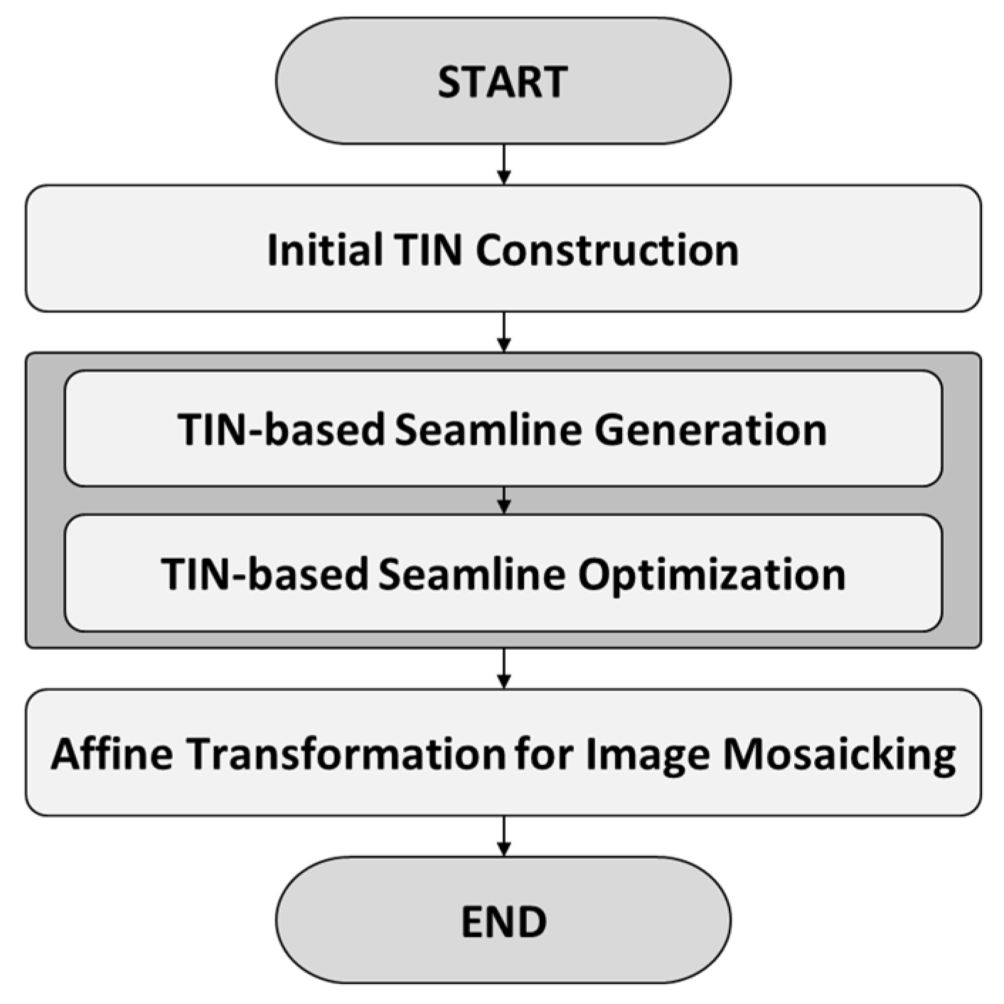
2. Materials and Methods

As shown in

Table 1. Descriptions of the dataset information.

Specification	Dataset 1	Dataset 2	Dataset 3
Platform	SmartOne	KD-2 Mapper	Phantom4 RTK
Manufacturer (City, Country)	Smartplanes (Jävrebyn, Sweden)	Keva Drone (Daejeon, Republic of Korea)	DJI (Shenzhen, China)
Flight type	fixed wing	fixed wing	rotary wing
Number of images	56	60	118
Image size (pixel)	4928 × 3264	7952 × 5304	5472 × 3648
Overlap (%)	end: 70, side: 80	end: 70, side: 80	end: 75, side: 85
Height of flight (m)	150	180	180
GSD 1 (m)	0.0389	0.0242	0.0492

¹ This is short for ground sample distance.

, we used three datasets for our study. The UAVs used in Datasets 1 and 2 are fixed-wing type. For Dataset 1, the UAV flew at a height of 150 m and acquired 56 images, with a ground sample distance (GSD) of 3.89 cm. For Dataset 2, the UAV acquired 60 images at a height of 180 m, with a GSD of 2.42 cm. The UAV used in Dataset 3 is a rotary wing type. The UAV acquired 118 images at a height of 180 m, with a GSD of 4.92 cm. The target areas for all datasets are plain and contain a few large buildings.

Figure 1 is a flowchart of our proposed method. First, tiepoints are generated from images. Tiepoints are determined between neighboring images and extracted by the SURF algorithm. Then, exterior orientation parameters (EOPs) of the images are corrected and 3D ground coordinates of each tiepoint are calculated by bundle adjustment. Next, a TIN is generated according to the ground coordinates of tiepoints extracted. Triangular facets in the TIN are projected to each image. Vertexes of the facets become the initial seamlines. Facet slopes are then calculated to detect error-prone facets. The facets with higher slopes are selected through slope angle thresholding, and the initial error-prone regions are determined through TIN facet clustering. The regions that may cause a mismatch error are then selected as the final error-prone regions. Next, the optimal images to process each error-prone region are selected, and the minimal images required to generate the mosaic are selected. Then, a facet-by-facet mosaicking is performed along the optimized seamlines. The details are described in the following subsections.

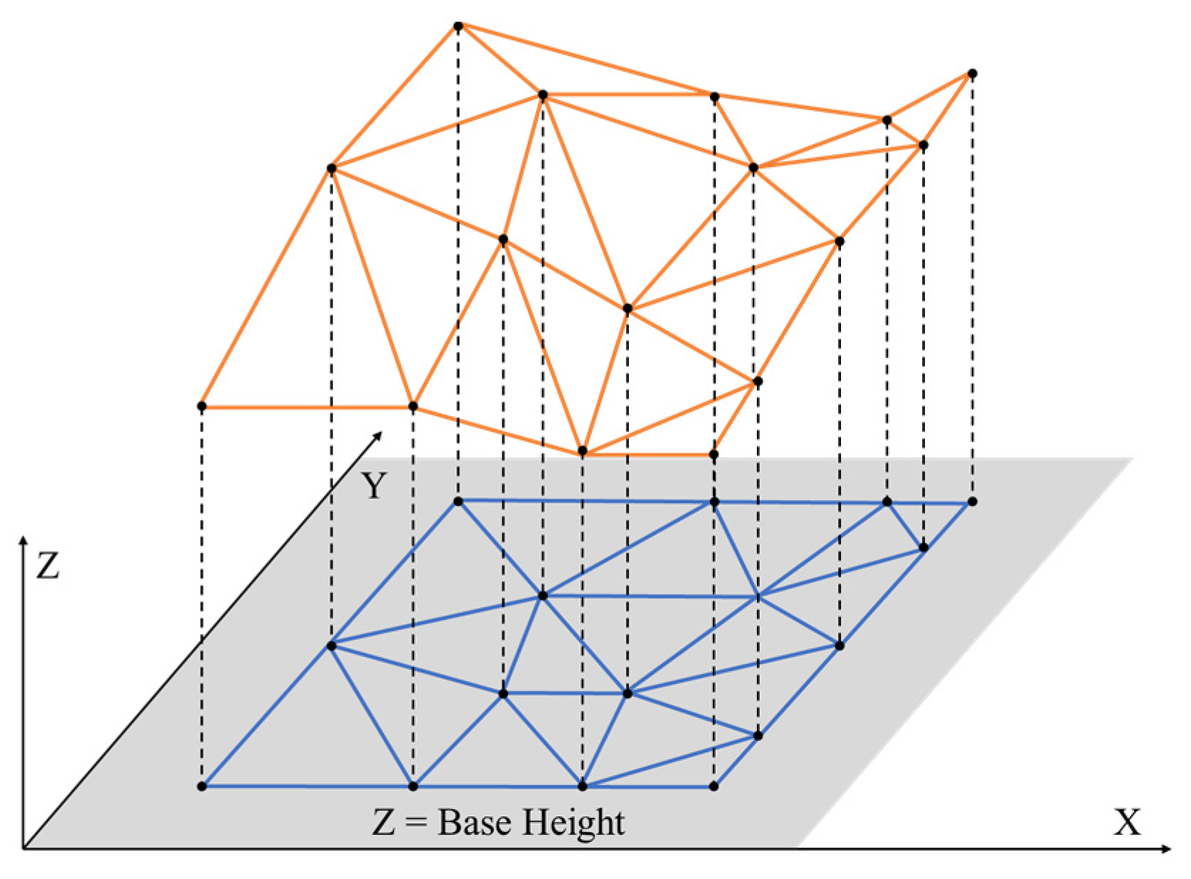
2.1. Initial TIN Construction

Since UAV datasets usually have a very large number of images, it is important to explore candidate images before processing. A tiepoint is a common feature defined in an overlap region between neighboring images. Therefore, it is desirable that tiepoint extraction is only attempted between pair images with overlapping regions. In this study, the ground coordinates of four corner points of an image are first calculated using the collinearity model, as shown in Equation (1). The initial EOPs and reference height are applied to this model, and the ground coverage of the image is determined.

$$\begin{gathered} X_P=\frac{r_{11}{x}_p+r_{12}{y}_p-r_{13}f}{r_{31}{x}_p+r_{32}{y}_p-r_{33}f}{(Z}_P-Z)+X \\ {Y}_P=\frac{r_{21}{x}_p+r_{22}{y}_p-r_{23}f}{r_{31}{x}_p+r_{32}{y}_p-r_{33}f}{(Z}_P-Z)+Y \end{gathered}$$

(1)

where $X, Y, Z$ are the position elements of the EOPs, $r_{11}~r_{33}$ are the rotation elements for the EOPs, $x_p,y_p$ are the coordinates of a point $p$ in the image, and $X_P,Y_P, Z_P$ are the ground coordinates projected from the point $p$ to point $P$.

From the ground coordinates of the four corner points, the ground coverage is calculated, and the overlapped relationships between the images are determined. Only up to 10 images are selected as candidate pairs for tiepoint extraction, in order of increasing overlap for a single image. Since our previous study, we have been using the SURF algorithm to extract tiepoints. The SURF algorithm is relatively robust to differences in scale and brightness of images [18]. In addition, it has similar performance to scale-invariant feature transform (SIFT) [19] with faster processing speed. In our previous study, we compared the performance of the SURF, and oriented features from accelerated segment test and rotated binary robust independent elementary feature (ORB) [20] algorithms in terms of tiepoint extraction quantity and processing time. On average, for images acquired in a rural area, the SURF algorithm was 0.1 s slower per image pair than the ORB algorithm, but generated 46 times as many triple tiepoints for bundle adjustment.

Bundle adjustment is a technique that simultaneously corrects EOPs of all UAV images and 3D ground coordinates of the tiepoints. Since bundle adjustment is performed by analyzing the positional relationship between tiepoints, their qualities affect the bundle adjustment accuracy. In this study, the random sample consensus (RANSAC) algorithm based on the coplanarity model is applied. The RANSAC algorithm randomly samples tiepoints and uses them to construct a coplanarity model [21]. It then calculates the Y-parallaxes of all tiepoints, which is the red arrow in Figure 2. The Y-parallax was calculated from each pairwise tiepoint on the image pair rectified according to the coplanarity model as in the triangular area of Figure 2. Tiepoints with errors of 3 pixels or more are classified as outliers and removed from the initial tiepoints.

The ground coordinates of the tiepoints are then projected onto an image according to the collinearity model in Equation (2). The difference between the projected and the original coordinates is calculated as the reprojection error according to Equation (3), as shown in the red arrow of Figure 3. In this figure, the yellow line is the observation vector from the projection center of $O_1$, $O_3$ to determine a ground point, the green line is the observation vector that projects the ground point back to $O_2$. Tiepoints within 3 pixels of the reprojection error are classified as inliers.

$$\begin{gathered} x_n=-f\frac{r_{11}\left(X_n-T_x\right)+r_{12}\left(Y_n-T_y\right)+r_{13}\left(Z_n-T_z\right)}{r_{31}\left(X_n-T_x\right)+r_{32}\left(Y_n-T_y\right)+r_{33}\left(Z_n-T_z\right)} \\ {y}_n=-f\frac{r_{21}\left(X_n-T_x\right)+r_{22}\left(Y_n-T_y\right)+r_{23}\left(Z_n-T_z\right)}{r_{31}\left(X_n-T_x\right)+r_{32}\left(Y_n-T_y\right)+r_{33}\left(Z_n-T_z\right)} \end{gathered}$$

(2)

$$d=\sqrt{{\left(\acute{x_n}-x_n\right)}^2+{\left(\acute{y_n}-y_n\right)}^2}$$

(3)

In the above equations, $f$ is the focal length, $n$ is the number of tiepoints from 1, $X_n,Y_n,Z_n$ are the ground coordinates of the tiepoints, $T_x,T_y,T_z$ are the position elements of the EOPs, $r_{11}~r_{33}$ are the rotation elements for the EOPs, $\acute{x_n}, \acute{y_n}$ are the image coordinates of the original tiepoint, $x_n, y_n$ are the image coordinates of the projected tiepoints, and $d$ is the reprojection error. The collinearity condition of Equation (1) is adopted as the model for bundle adjustment. To correct the EOPs of all images simultaneously, the collinearity models for all inlier tiepoints are included. Adjustment is performed with recursive least squares [22]. Through bundle adjustment, ground coordinates of tiepoints are estimated.

The terrain features where relief displacement occurs have different shapes in different UAV images. Therefore, relief displacement is a major source of mosaic error [23]. Since relief displacement is determined by the height of terrain features, it can be detected by utilizing a terrain model. TIN is a model that can represent terrain with discontinuously acquired height information, such as ground or elevation points. Based on the Delaunay triangulation algorithm, three ground points are grouped together to form a triangle [24], and the angle and direction of the slope can be calculated from the three points of the triangle. Although it is less accurate than DSM, it is simpler and faster to utilize for image mosaicking because the entire terrain can be reconstructed with only the height information of a few points.

In this paper, the adjusted tiepoints with 3D ground coordinates are defined as initial point clouds. Based on the initial point clouds, a TIN in the model space is formed, as shown in Figure 4. A TIN is created based on the Delaunay triangulation, where each node contains information of the initial point clouds. The two outmost layers of the TIN are excluded from the computation because there are too many sharp triangles on the outer layer of the TIN. Next, the slopes of the TIN facets are calculated. When the three nodes of a facet are $P_1\left(x_1,y_1,z_1\right),P_2\left(x_2,y_2,z_2\right),P_3\left(x_3,y_3,z_3\right)$, the normal vector of the facet is calculated according to Equation (4). The slope of the facet is calculated as the angle between this normal vector and the reference plane. This is shown in Equation (5).

$$\overrightarrow{n}=\left[\begin{array}{c}{n}_1\\ n_2\\ n_3\end{array}\right]=\overrightarrow{P_1{P}_2}\times \overrightarrow{P_1{P}_3}=\left[\begin{array}{c}\left(y_2-y_1\right)\left(z_3-z_1\right)-\left(z_2-z_1\right)\left(y_3-y_1\right)\\ \left(z_2-z_1\right)\left(x_3-x_1\right)-\left(x_2-x_1\right)\left(z_3-z_1\right)\\ \left(x_2-x_1\right)\left(y_3-y_1\right)-\left(y_2-y_1\right)\left(x_3-x_1\right)\end{array}\right]$$

(4)

$$\theta =\frac{\pi }{2}-{\mathit{cos}}^{-1}\left(\frac{n_1^2+n_2^2}{\sqrt{n_1^2+n_2^2+n_3^2}\sqrt{n_1^2+n_2^2}}\right)$$

(5)

where $\overrightarrow{n}$ is the normal vector of the facet, $n_1,n_2,n_3$ are the elements of the normal vector, and $\theta$ is the slope of the facet.

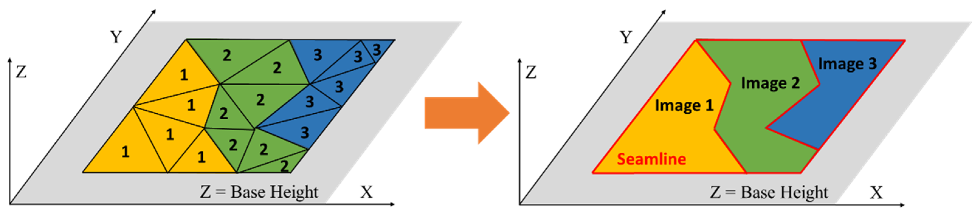
2.2. TIN-Based Seamline Generation

The nodes of the TIN facets in our study contain the multiple image points and a single ground point information of the point cloud. As shown in the left image of Figure 5, the image information that the three nodes of a facet have in common become the image information of the facet. In the left image of Figure 5, the numbers are examples of the image IDs assigned. TIN facets are clustered by image, and their areas determine the mosaic extent for each image. In Figure 5, the yellow, green, and blue colors represent examples of the mosaic extent for each image.

To improve the speed of mosaicking, mosaic overlaps of images are first checked. The mosaic overlap of an image is calculated by dividing the area of the facets overlapped with other images by the total area of the assigned facets. Then, images with high mosaic overlap are excluded from mosaicking. The mosaic overlap check is repeated for each strip of the UAV image. By performing the computation for all UAV image strips, only the minimal images needed for mosaicking are selected. The mosaic seamlines of the selected images are defined as the outlines of the assigned facets. This is shown on the right side of Figure 5.

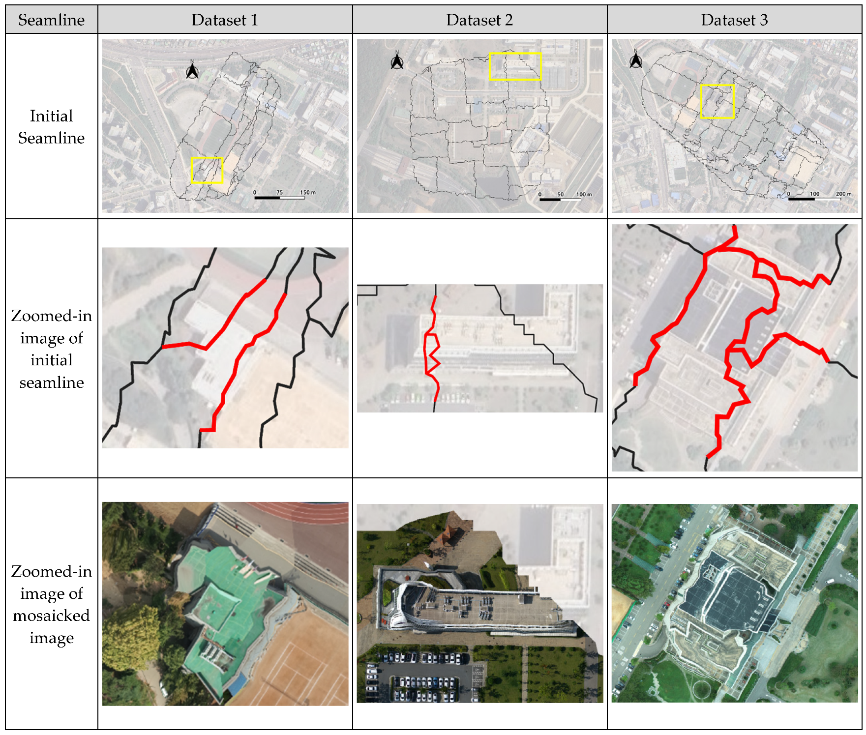
2.3. TIN-Based Seamline Optimization

Figure 6 shows a schema for error-prone region detection. As described in the introduction, errors in the mosaic occur in the facets with high slope angles. First, by slope angle thresholding, facets with higher slopes are extracted. The extracted facets form several clusters around ground objects such as buildings or trees. In this paper, these clustered regions are defined as error-prone regions.

The area of a single error-prone region is calculated according to Equation (6),

$$A=\sum _{n=1}^T\frac{\left|\overrightarrow{P_{n_1}{P}_{n_2}}·\overrightarrow{P_{n_1}{P}_{n_3}}\right|}{2}=\sum _{n=1}^T\frac{\left|\left(x_{n_2}-x_{n_1}\right)\left(y_{n_3}-y_{n_1}\right)-\left(x_{n_3}-x_{n_1}\right)\left(y_{n_2}-y_{n_1}\right)\right|}{2}$$

(6)

where $A$ is the area of the target region, $T$ is the total number of facets on the target region, and $P_{n_{1 to 3}}\left(x, y,z\right)$ represents the three nodes of the $n$-th facet.

The initial error-prone region may contain very small regions with few errors. Therefore, only error-prone regions with large areas are targeted for optimization. In the proposed algorithm, the facets of a TIN are used to determine the seamline and to generate image patches for mosaicking. To avoid stitching between different images on the error-prone region, vertices located inside the region are excluded from being selected as seamlines. Through this method, one patch region is mosaicked using only one image. The image used should cover as much of the region as possible and have as small a relief displacement as possible about the error-causing object.

Equation (7) is for calculating the unsuitability of an image for an error-prone region,

$$S_{m,n}=W_p\sqrt{{\left(x_{m_p}-x_n\right)}^2+{\left(y_{m_p}-y_n\right)}^2}+W_{\mathrm{c}}\sqrt{{\left(x_{m_c}-x_n\right)}^2+{\left(y_{m_c}-y_n\right)}^2}$$

(7)

where $S_{m,n}$ is the unsuitability of the $m$-th image for the $n$-th error-prone region, $x_{m_p}, y_{m_p}$ are the principal points of the $m$-th image, $x_{m_c}, y_{m_c}$ are the image coordinates of the vertical projection of the projection center of the $m$-th image, $x_n, y_n$ are the image coordinates of the center of gravity of the $n$-th error-prone region, $W_p$ is the weight of the distance from the principal point to $x_n, y_n$, and $W_{\mathrm{c}}$ is the weight of the distance from the projection center to $x_n, y_n$.

Both the distance from the principal point and the distance from the projection center in the image are considered to select an optimal image for the error-prone region. In order to avoid seamlines forming above an error-prone region, it is important that the error-prone region be covered in one image as much as possible. Therefore, we set $W_p$ to be larger than $W_c$ to search an optimal image where the error-prone region is close to the image principal point. The $m$-th image with the smallest $S_{m,n}$ is selected as the best image for the $n$-th error-prone region.

2.4. Affine Transformation for Image Mosaicking

As shown in Figure 7, facets of a TIN become image patches for mosaicking. The transformation relationship from the original image to the mosaic is estimated according to the affine transformation model in Equation (8).

$$\left[\begin{array}{c}x\prime \\ y\prime \\ 1\end{array}\right]=\left[\begin{array}{ccc}{r}_1& r_2& t_1\\ r_3& r_4& t_2\\ 0& 0& 1\end{array}\right]\left[\begin{array}{c}x\\ y\\ 1\end{array}\right]$$

(8)

where $x,y$ are the coordinates of the original image, $x^{\prime },y^{\prime }$ are the coordinates of the transformed image, $r_i$ is the rotation factors of the affine transformation model, and $t_j$ is the translation factors of the affine transformation model. Affine transformation is a model for analyzing parallel translation, rotation, scaling, and shearing of objects [25]. Since the affine transformation has 6 degrees of freedom, the transformation coefficients can be estimated from three or more tiepoints. Along the estimated transformation coefficients, the image patches are warped and stitched into a mosaic. The image mosaicking is first performed on the optimal images for the error-prone regions. The mosaicking is then performed on the minimal images determined by the operation optimization to produce the final mosaicked image.

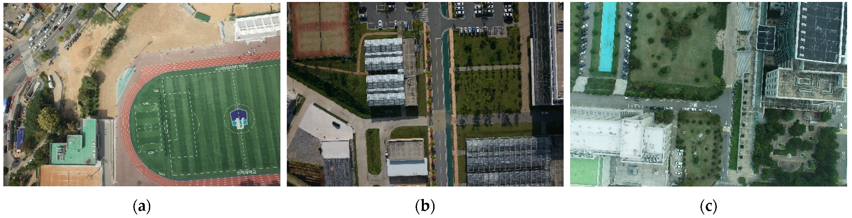
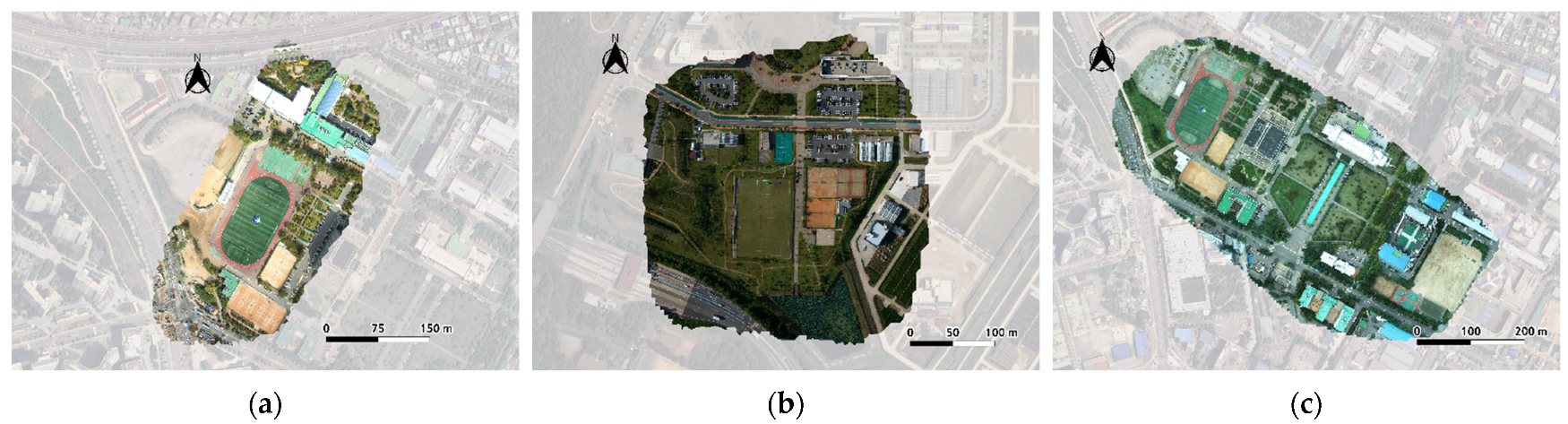
3. Experiment Results

Figure 8 shows sample UAV images for the three datasets used in this study. Dataset 1 was acquired over Inha University campus and covered an area of 350 m by 470 m. The area of Dataset 1 had a slight north–south sloping terrain. A playground is in the center of Dataset 1 and buildings are located around it. Dataset 2 had an area of 350 m by 380 m, and its terrain is flat. The buildings in Dataset 2 have moderate height among the three datasets. Dataset 3 was also acquired over Inha University campus. The area of Dataset 3 is the largest, at 740 m by 585 m. It contained many buildings, some of which were larger than 5000 square meters.

In this study, we presented the initial TIN construction results, TIN-based seamline generation results, TIN-based seamline optimization results, and final mosaic results. We applied relative radiometric correction to the UAV images [26,27]. Our relative radiometric correction method uses image tiepoints without an irradiance sensor. It constructed image network-based tiepoints and estimated coefficients of relative radiometric correction between images by interpreting the relationship between the brightness values of the tiepoints. Finally, our method applied image blending to keep color consistency. By removing non-geometric error factors such as lighting conditions and sensor quality, the results were compared to the results of commercial software only for geometric errors, as possible. The commercial software used for comparison is Pix4Dmapper in version 4.5.6. This software is one of the most popular software packages for UAV image processing [28].

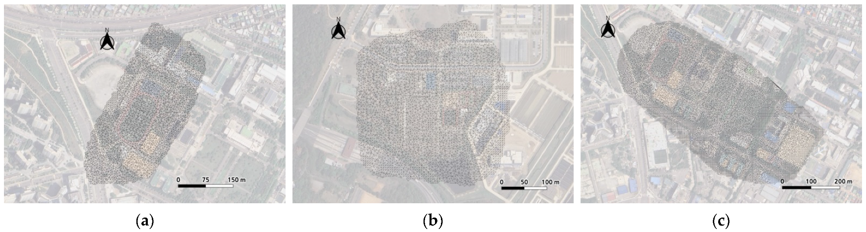
3.1. Results of Intial TIN Construction

Table 2. Results of initial point cloud generation.

Dataset Name	Dataset 1	Dataset 2	Dataset 3
Number of candidate tiepoints	73,294	112,451	175,615
Number of initial point clouds	39,041	65,555	53,062
Initial point cloud conversion ratio (%)	53.27	58.30	30.22
Reprojection error of initial point cloud (pixel)	0.9316	1.0243	0.9869

shows the results of initial point cloud generation by bundle adjustment. A total of 73,294 candidate tiepoints were extracted for Dataset 1, 112,451 for Dataset 2, and 175,615 for Dataset 3. These candidate tiepoints were checked for outlier removal. The tiepoints that satisfied the tolerance of reprojection error were classified into the initial point cloud. The conversion rate to initial point clouds ranged from 30% to 60%. For Dataset 1, 39,041 initial point clouds were determined, 65,555 for Dataset 2, and 53,062 for Dataset 3. The initial point clouds for all three datasets had a small reprojection error of about 1 pixel. Finally, ground coordinates of these initial point clouds were determined through bundle adjustment.

Table 3. Results of TIN construction.

Dataset Name	Dataset 1	Dataset 2	Dataset 3
Number of sampled point clouds	3922	4614	10,009
Number of TIN facets	7112	8465	18,936
Processing time for point cloud sampling and TIN construction (seconds)	1.35	0.39	0.55

shows the results of TIN construction using the initial point clouds. First, the initial dense point cloud was reduced by bucketing for TIN generation with a moderate number of facets [17]. For Dataset 1, 3922 points were sampled from the initial point cloud. For Dataset 2, 4614 points were sampled, and for Dataset 3, 10,009 points were sampled. A TIN was built utilizing only the sampled points. The number of facets in the constructed TINs was 7112 for Dataset 1, 8465 for Dataset 2, and 18,936 for Dataset 3. The process of bucket sampling from the initial point cloud and building the TINs was fast, totaling about 1 s for all three datasets. Figure 9 shows the generated TINs on a basemap. The sampled TIN facets were uniformly distributed across the study area.

3.2. Results of TIN-Based Seamline Generation

Figure 10 shows initial mosaic seamlines built from the TINs in Figure 9 before applying seamline optimization. The top images in Figure 10 show the overall seamlines. The yellow boxes are zoomed in the middle in Figure 10. The initial seamlines were formed along the outline of the TIN in each image. Some seamlines appeared to cross over buildings. The yellow boxed areas indicate areas where seamlines crossed buildings, and the red lines in the figure mark those seamlines. The initial mosaicked results over the yellow boxes are shown in the bottom images of Figure 10. These results generated from initial seamlines contained severe seamline mismatches. In the seamline optimization of the next step, the yellow boxed areas are used as targets for improvement.

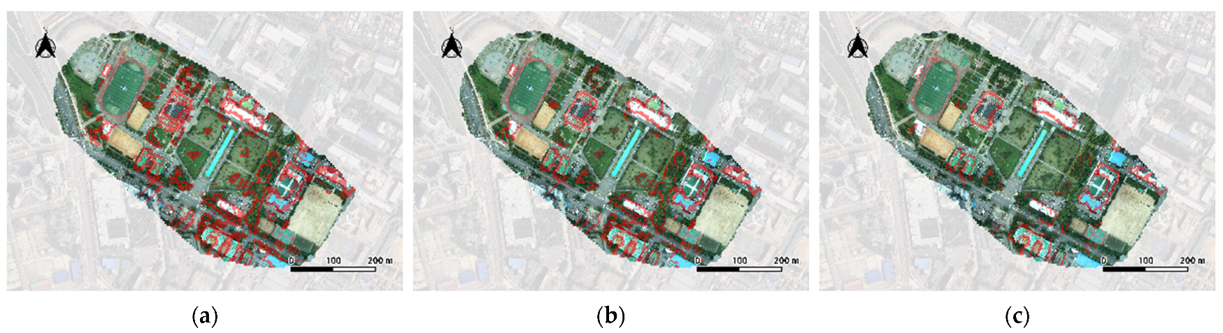
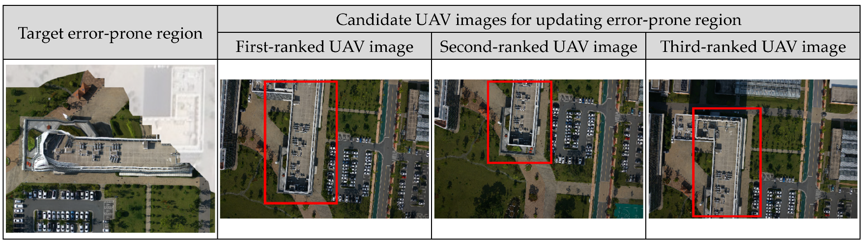
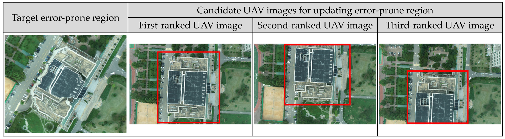
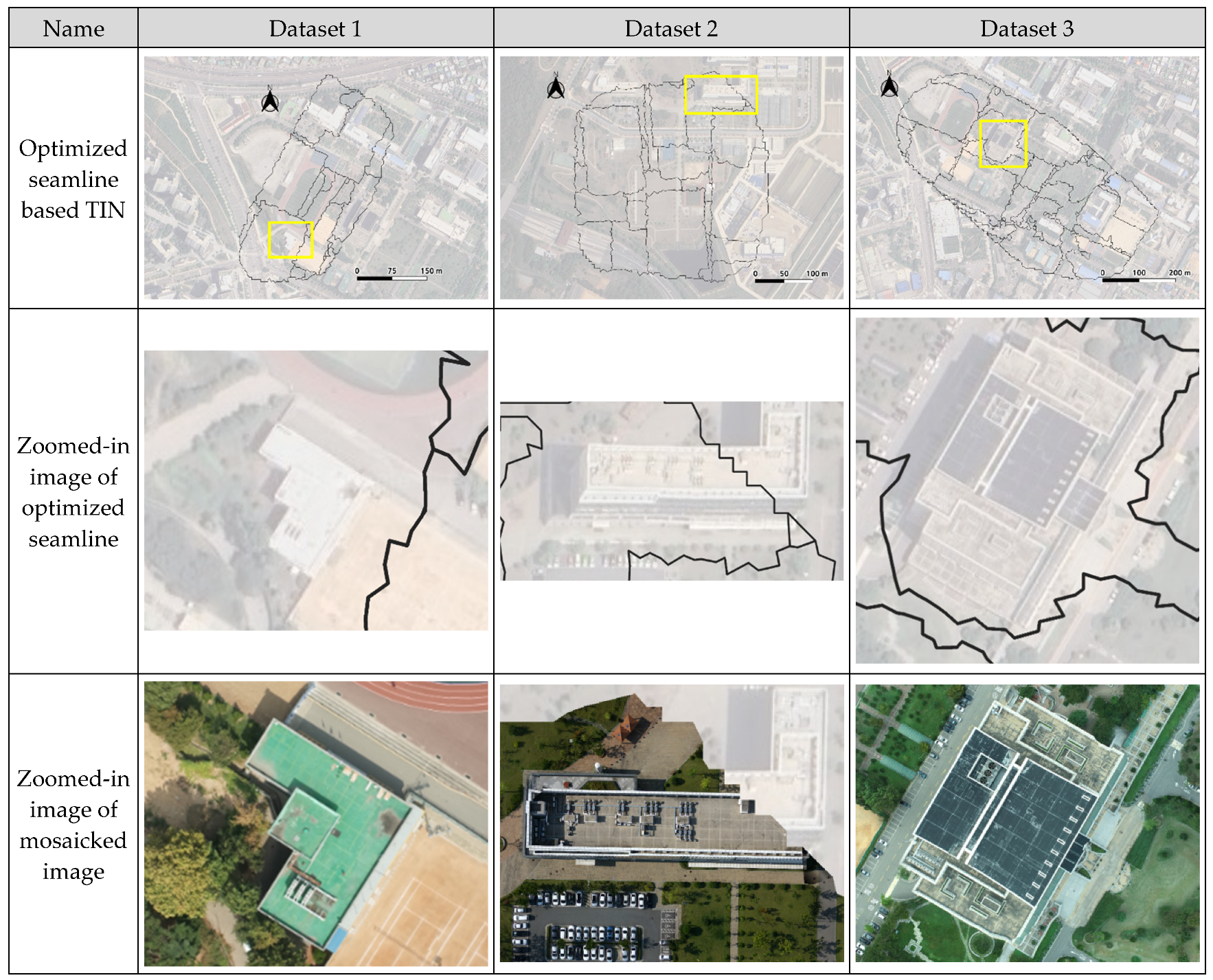
3.3. Results of TIN-Based Seamline Optimization

Figure 11 shows the slope angles of TIN facets for Dataset 1 through Dataset 3. The slope angles range from 0 to 90 degrees, with lighter colors representing higher angles in this figure. Most slope angles were lower on flat areas such as playgrounds and higher around buildings and trees. Some slope angles were slightly higher in flat areas. These results indicated that the self-generated TINs were a relatively successful representation of the real terrain.

Figure 12, Figure 13 and Figure 14 show the initial mosaicked images. In these figures, the red areas indicate the error-prone regions detected by the slope angle thresholding. Figure (a) of the three figures shows the detected facets at a threshold of 30 degrees in the initial mosaicked image. The detected facets were evenly distributed around low objects such as cars and shrubs. Moreover, some facets were detected in error regions where the slope angle was different from the real terrain. This indicated that some areas that did not have mosaic errors by relief displacement were also detected at the 30-degree slope angle thresholding. Figure (b) of the three figures shows the detected facets at a threshold of 45 degrees in the initial mosaicked image. The detected facets were distributed around the building and included most of the mosaic error areas of noticeable relief displacement. With a threshold of 60 degrees, facets were detected mainly around tall buildings, as in Figure (c) of the three figures. Some of the error regions in the initial mosaicked image were not detected by slope thresholding. Therefore, the facets detected at a threshold of 45 degrees were determined as error-prone regions in this study.

Figure 15, Figure 16 and Figure 17 show the target error-prone regions defined in Section 3.2 and the selection process of the candidate UAV images for updating these regions. In the figures, candidate images are shown by their ranks. The red boxes in the figure show the target error-prone regions in the original images. In the first-ranked candidate images, the target error-prone region was located in the center of the images. These images were acquired close to perpendicular, so the façades of buildings were not featured significantly in the images. In contrast, in the second- and third-ranked candidate images, the target error-prone region was relatively far from the center of the image. For Datasets 2 and 3, the target error-prone region was even out of the image area. The unsuitabilites of the candidate images are shown in

Table 4. Unsuitability of candidate UAV images for target error-prone region.

Name	Ranked	Unsuitability (Pixels)
Dataset 1	1	477.83
	2	521.74
	3	606.03
Dataset 2	1	691.68
	2	1309.21
	3	1427.27
Dataset 3	1	97.98
	2	509.69
	3	679.41

. For Dataset 1, the unsuitabilites of the three candidate images were not significantly different. This is because the target error-prone regions were not out of the image area in all three candidate images. For Datasets 2 and 3, the difference in unsuitability between the first-ranked candidate image and the rest of the candidate images was significant. In the first-ranked candidate image, the target error-prone region was centered in the image, whereas in the remaining candidate images, it was outside the range of the image. These results indicate that it is possible to automatically determine the best images for error-prone region improvement based on the unsuitability proposed here.

Figure 18 shows the seamlines and mosaicked images improved by seamline optimization. The top images in Figure 18 show the overall seamlines, and the middle images are zoomed in on the yellow box in the top images. To verify the improvement, we visually compared the initial seamline in Figure 10 to the optimized seamline in Figure 18. Unlike the initial seamlines, the improved seamlines were formed by avoiding the error-prone areas detected at the 45-degree threshold, as in Figure 12, Figure 13 and Figure 14. Furthermore, as shown in the yellow box in Figure 18, the error-prone regions were almost centered in one image. By stitching the error-prone regions into a single image, no mismatches or distortions occurred in those regions, unlike the initial mosaicked image, as in Figure 10.

Table 5. Mosaic errors according to seamline optimization.

Name	Method	Mosaic Error (Pixels)
Dataset 1	Image mosaicking without seamline optimization	22.5521
	Image mosaicking with seamline optimization	1.0929
Dataset 2	Image mosaicking without seamline optimization	11.6237
	Image mosaicking with seamline optimization	0.9848
Dataset 3	Image mosaicking without seamline optimization	31.7093
	Image mosaicking with seamline optimization	2.1861

shows the improvement in mosaic error by seamline optimization. The mosaic error was calculated as the distance between the position of the TIN nodes calculated by the affine transformation and the position of the actual point cloud on the mosaic space. For Dataset 1, the initial mosaicked image without seamline optimization had a mosaic error of 22.5521 pixels. Seamline optimization then removed the mosaic error by relief displacement, resulting in a final mosaicked image with a mosaic error of only 1.0929 pixels. For Dataset 2, which contains lower buildings, the initial mosaic had a relatively small error of 11.6237 pixels. The final mosaic then had an error of 0.9848 pixels, an improvement of about 10 pixels. For Dataset 3, which contains many tall buildings, the initial mosaic image had the largest error of 31.7093 pixels. Nevertheless, the seamline optimization reduced the mosaic error to about 2 pixels. These results indicated that the TIN-based seamline optimization effectively eliminated the mosaic errors by relief displacement, which is the major source of mosaic error. This was consistent with the visual analysis in Figure 10 and Figure 18.

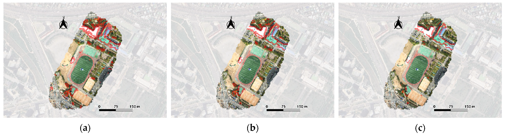
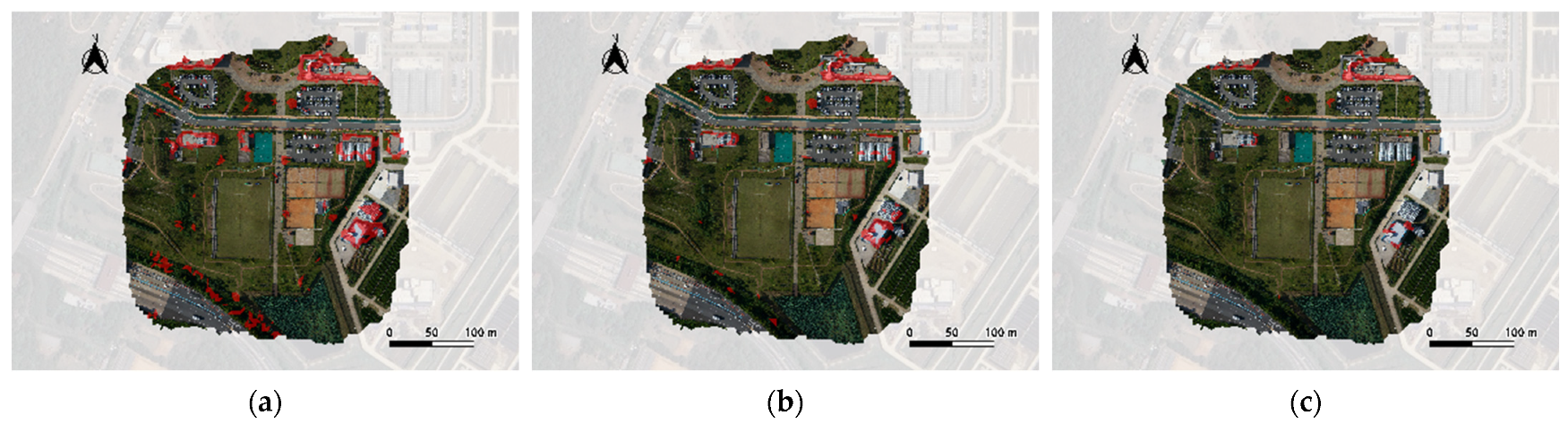
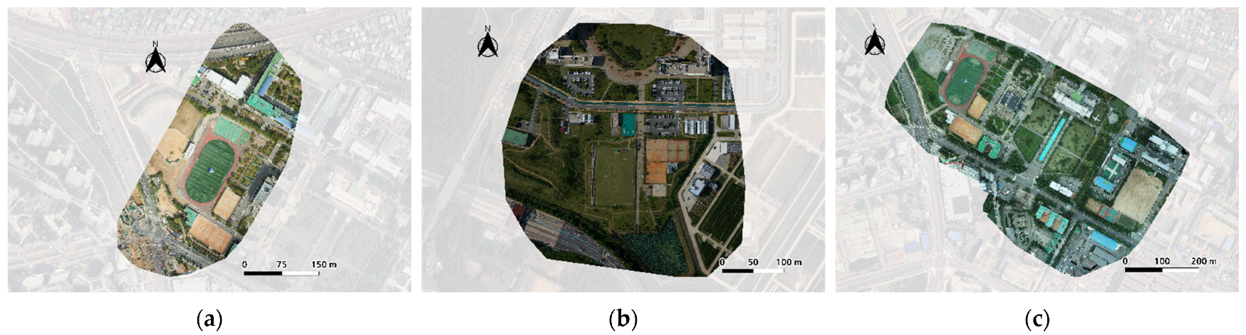
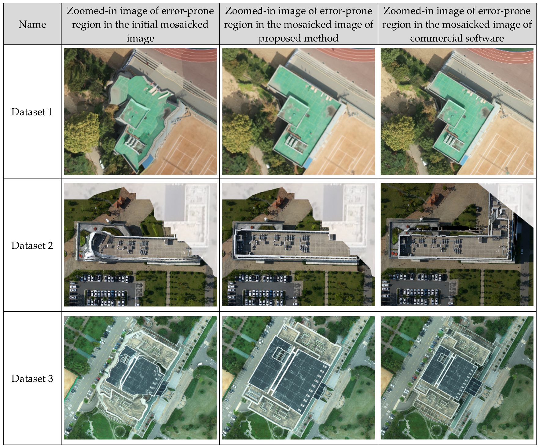
3.4. Final Results and Discussion

Figure 19 shows the final mosaicked images of the proposed method. These mosaicked images were reconstructed along the optimized seamlines. Unlike the initial mosaicked images as Figure 12, Figure 13 and Figure 14, most of the mosaic errors were eliminated on the final mosaicked images. Figure 20 shows mosaicked images created by commercial software. For the target error-prone area defined in Figure 10, mosaicking results from the initial seamlines, the optimized seamlines, and a commercial software are shown in Figure 21.

It is notable that the commercial software generated orthoimages using a terrain-based technique. Nevertheless, our mosaicked images showed similar quality to the mosaicked images produced by the commercial software. For Dataset 1, neither our optimal mosaicked image nor the image from the commercial software had any mosaic errors in the error-prone regions. For Dataset 2, the commercial software’s mosaicked image had a slight mismatch, but our mosaicked image did not have any mosaic errors. For Dataset 3, both methods produced no mosaic errors. These results indicated that our proposed image-based technique could have similar quality to the terrain-based method.

Table 6. Processing times for mosaicking of proposed method and commercial software.

Name	Method	Processing Time for Mosaicking
Dataset 1	Proposed method	8 s
	Commercial software	14 min 36 s
Dataset 2	Proposed method	16 s
	Commercial software	29 min 21 s
Dataset 3	Proposed method	24 s
	Commercial software	29 min 34 s

shows the processing times of our proposed method and commercial software. These processing times were the sum of the whole process required for mosaicking. Time for tiepoint extraction and bundle adjustment was not included. Since our proposed method performed all the processing of mosaicking using only images and tiepoints, our method worked very fast. For all three datasets, mosaicking was carried out within half a minute. In contrast, the commercial software performed mosaicking through DSM generation and orthorectification. This resulted in a slower processing time of 15 to 30 min.

Because our method excluded orthorectification from the image mosaicking, buildings appeared larger than they actually are. This effect was smaller in Dataset 1 and Dataset 2, but larger in Dataset 3, which has relatively tall buildings. Nevertheless, our method showed that it can quickly produce mosaicked images while minimizing errors of mismatch and distortion.

4. Conclusions

In this study, we proposed a high-speed UAV image mosaicking method that utilizes TIN based on self-generated tiepoints. The contribution of this study is to show that it is possible to minimize the mosaicking image error caused by relief displacement by optimizing the seamline based on TIN. Previous studies on image-based image mosaicking techniques mainly analyze the brightness of the image to solve the error caused by relief displacement. However, in this study, we utilized the slope of the TIN to detect the geometric errors. Through the slope angle analysis, it was possible to detect the areas of relief displacement on the terrain, and to confirm the possibility of eliminating the mosaic error by seamline optimization.

In this study, the error-prone areas were mosaicked into a single image to avoid the relief displacement error. For images taken by small UAV or at flight height, sometimes the entire error-prone area may not be contained in one image. Therefore, in future research, we plan to segment error-prone regions that are not covered by one image by considering the geometry between the error-prone regions and images. Nevertheless, we argue that the approach in this study is unique because we developed a new robust image mosaicking method against relief displacement based on a self-generated TIN. We expect that our proposed method can be presented as a fast and robust mosaicking technique against relief displacement.

References

1. Tsouros, D.C.; Bibi, S.; Sarigiannidis, P.G. A review on UAV-based applications for precision agriculture. Information 2019, 10, 349. [Google Scholar] [CrossRef]
2. Tsouros, D.C.; Triantafyllou, A.; Bibi, S.; Sarigannidis, P.G. Data acquisition and analysis methods in UAV-based applications for Precision Agriculture. In Proceedings of the 2019 15th International Conference on Distributed Computing in Sensor Systems (DCOSS), Santorini, Greece, 29–31 May 2019. [Google Scholar]
3. Chan, B.; Guan, H.; Jo, J.; Blumenstein, M. Towards UAV-based bridge inspection systems: A review and an application perspective. Struct. Monit. Maint. 2015, 2, 283–300. [Google Scholar] [CrossRef]
4. Rhee, S.; Kim, T.; Kim, J.; Kim, M.C.; Chang, H.J. DSM Generation and Accuracy Analysis from UAV Images on River-side Facilities. Korean J. Remote Sens. 2015, 31, 183–191. [Google Scholar] [CrossRef]
5. Park, S.; Park, N.W. Effects of class purity of training patch on classification performance of crop classification with convolutional neural network. Appl. Sci. 2020, 10, 3773. [Google Scholar] [CrossRef]
6. Avola, D.; Cinque, L.; Foresti, G.L.; Martinel, N.; Pannone, D.; Piciarelli, C. A UAV video dataset for mosaicking and change detection from low-altitude flights. IEEE Trans. Syst. Man Cybern. Syst. 2018, 50, 2139–2149. [Google Scholar] [CrossRef]
7. Li, X.; Feng, R.; Guan, X.; Shen, H.; Zhang, L. Remote sensing image mosaicking: Achievements and challenges. IEEE Geosci. Remote Sens. Mag. 2019, 7, 8–22. [Google Scholar] [CrossRef]
8. Li, T.; Jiang, C.; Bian, Z.; Wang, M.; Niu, X. A review of true orthophoto rectification algorithms. IOP Conf. Ser. Mater. Sci. Eng. 2019, 780, 022035. [Google Scholar] [CrossRef]
9. Shoab, M.; Singh, V.K.; Ravibabu, M.V. High-precise true digital orthoimage generation and accuracy assessment based on UAV images. J. Indian Soc. Remote Sens. 2021, 50, 613–622. [Google Scholar] [CrossRef]
10. Jiang, Y.; Bai, Y. Low–high orthoimage pairs-based 3D reconstruction for elevation determination using drone. J. Constr. Eng. Manag. 2021, 147, 04021097. [Google Scholar] [CrossRef]
11. Kim, J.I.; Kim, H.C.; Kim, T. Robust mosaicking of lightweight UAV images using hybrid image transformation modeling. Remote Sens. 2020, 12, 1002. [Google Scholar] [CrossRef]
12. Zhang, W.; Guo, B.; Li, M.; Liao, X.; Li, W. Improved seam-line searching algorithm for UAV image mosaic with optical flow. Sensors 2018, 18, 1214. [Google Scholar] [CrossRef]
13. Yuan, Y.; Fang, F.; Zhang, G. Superpixel-based seamless image stitching for UAV images. IEEE Trans. Geosci. Remote Sens. 2020, 59, 1565–1576. [Google Scholar] [CrossRef]
14. Yuan, S.; Yang, K.; Li, X.; Cai, H. Automatic seamline determination for urban image mosaicking based on road probability map from the D-LinkNet neural network. Sensors 2020, 20, 1832. [Google Scholar] [CrossRef]
15. Li, L.; Yao, J.; Liu, Y.; Yuan, W.; Shi, S.; Yuan, S. Optimal seamline detection for orthoimage mosaicking by combining deep convolutional neural network and graph cuts. Remote Sens. 2017, 9, 701. [Google Scholar] [CrossRef]
16. Dai, Q.; Fang, F.; Li, J.; Zhang, G.; Zhou, A. Edge-guided composition network for image stitching. Pattern Recognit. 2021, 118, 108019. [Google Scholar] [CrossRef]
17. Yoon, S.J.; Kim, T. Fast UAV Image Mosaicking by a Triangulated Irregular Network of Bucketed Tiepoints. Remote Sens. 2023, 15, 5782. [Google Scholar] [CrossRef]
18. Tareen, S.A.K.; Saleem, Z. A comparative analysis of sift, surf, kaze, akaze, orb, and brisk. In Proceedings of the 2018 International Conference on Computing, Mathematics and Engineering Technologies (iCoMET), Sukkur, Pakistan, 3–4 March 2018. [Google Scholar]
19. Liu, Y.; He, M.; Wang, Y.; Sun, Y.; Gao, X. Farmland aerial images fast-stitching method and application based on improved sift algorithm. IEEE Access 2022, 10, 95411–95424. [Google Scholar] [CrossRef]
20. Rublee, E.; Rabaud, V.; Konolige, K.; Bradski, G. ORB: An efficient alternative to SIFT or SURF. In Proceedings of the 2011 International Conference on Computer Vision, Barcelona, Spain, 6–13 November 2011. [Google Scholar]
21. Wu, F.L.; Fang, X.Y. An improved RANSAC homography algorithm for feature based image mosaic. In Proceedings of the 7th WSEAS International Conference on Signal Processing, Computational Geometry & Artificial Vision, Athens, Greece, 24–26 August 2007; pp. 202–207. [Google Scholar]
22. Thompson, M.M.; Eller, R.C.; Radlinski, W.A.; Speert, J.L. Manual of Photogrammetry, 6th ed.; American Society for Photogrammetry and Remote Sensing (ASPRS): Falls Church, VA, USA, 2013; pp. 121–159. [Google Scholar]
23. Lin, Y.C.; Zhou, T.; Wang, T.; Crawford, M.; Habib, A. New orthophoto generation strategies from UAV and ground remote sensing platforms for high-throughput phenotyping. Remote Sens. 2021, 13, 860. [Google Scholar] [CrossRef]
24. Park, D.; Cho, H.; Kim, Y. A TIN compression method using Delaunay triangulation. Int. J. Geogr. Inf. Sci. 2001, 15, 255–269. [Google Scholar] [CrossRef]
25. Zheng, J.; Wang, Y.; Wang, H.; Li, B.; Hu, H.M. A novel projective-consistent plane based image stitching method. IEEE Trans. Multimed. 2019, 21, 2561–2575. [Google Scholar] [CrossRef]
26. Shin, J.I.; Cho, Y.M.; Lim, P.C.; Lee, H.M.; Ahn, H.Y.; Park, C.W.; Kim, T. Relative radiometric calibration using tie points and optimal path selection for UAV images. Remote Sens. 2020, 12, 1726. [Google Scholar] [CrossRef]
27. Ban, S.; Kim, T. Relative Radiometric Calibration of UAV Images for Image Mosaicking. Int. Arch. Photogramm. Remote Sens. Spat. Inf. Sci. 2022, 43, 361–366. [Google Scholar] [CrossRef]
28. Jarahizadeh, S.; Salehi, B. A Comparative Analysis of UAV Photogrammetric Software Performance for Forest 3D Modeling: A Case Study Using AgiSoft Photoscan, PIX4DMapper, and DJI Terra. Sensors 2024, 24, 286. [Google Scholar] [CrossRef]
Figure 1. Flowchart of proposed method.
Remotesensing 16 01738 g001
Figure 2. Concept for Y-parallaxes on epipolar geometry.
Remotesensing 16 01738 g002
Figure 3. Concept for photogrammetric reprojection error.
Remotesensing 16 01738 g003
Figure 4. Concept for TIN generation using initial point clouds.
Remotesensing 16 01738 g004
Figure 5. Concept for TIN facet assignment to the images.
Remotesensing 16 01738 g005
Figure 6. Scheme for error-prone region detection.
Remotesensing 16 01738 g006
Figure 7. Affine transformation-based mosaicking on TIN facet.
Remotesensing 16 01738 g007
Figure 8. Sample UAV images for (a) Dataset 1; (b) Dataset 2; (c) Dataset 3.
Remotesensing 16 01738 g008
Figure 9. Results of TIN generation on satellite basemap: (a) TIN for Dataset 1; (b) TIN for Dataset 2; (c) TIN for Dataset 3.
Remotesensing 16 01738 g009
Figure 10. Results of seamline generation for overall region of interest (upper images), for enlarged regions shown as yellow boxes (middle images), and mosaicked image for enlarged regions (bottom images).
Remotesensing 16 01738 g010
Figure 11. Slope angles of TIN facets for (a) Dataset 1; (b) Dataset 2; (c) Dataset 3.
Remotesensing 16 01738 g011
Figure 12. Error-prone regions detected for Dataset 1 (a) at a threshold of 30°; (b) at a threshold of 45°; (c) at a threshold of 60°.
Remotesensing 16 01738 g012
Figure 13. Error-prone regions detected for Dataset 2 (a) at a threshold of 30°; (b) at a threshold of 45°; (c) at a threshold of 60°.
Remotesensing 16 01738 g013
Figure 14. Error-prone regions detected for Dataset 3 (a) at a threshold of 30°; (b) at a threshold of 45°; (c) at a threshold of 60°.
Remotesensing 16 01738 g014
Figure 15. Target error-prone region and candidate UAV images for improvement for Dataset 1.
Remotesensing 16 01738 g015
Figure 16. Target error-prone region and candidate UAV images for improvement for Dataset 2.
Remotesensing 16 01738 g016
Figure 17. Target error-prone region and candidate UAV images for improvement for Dataset 3.
Remotesensing 16 01738 g017
Figure 18. Results of seamline optimization for overall region of interest (upper images), for enlarged regions shown as yellow boxes (middle images), and mosaicked image for enlarged regions (bottom images).
Remotesensing 16 01738 g018
Figure 19. Final mosaicked image by proposed method (a) for Dataset 1; (b) for Dataset 2; (c) for Dataset 3.
Remotesensing 16 01738 g019
Figure 20. Mosaicked image generated by commercial software (a) for Dataset 1; (b) for Dataset 2; (c) for Dataset 3.
Remotesensing 16 01738 g020
Figure 21. Comparison of error-prone region in the mosaicked image of proposed method and commercial software.
Remotesensing 16 01738 g021