All articles published by MDPI are made immediately available worldwide under an open access license. No special
permission is required to reuse all or part of the article published by MDPI, including figures and tables. For
articles published under an open access Creative Common CC BY license, any part of the article may be reused without
permission provided that the original article is clearly cited. For more information, please refer to
https://www.mdpi.com/openaccess.
Feature papers represent the most advanced research with significant potential for high impact in the field. A Feature
Paper should be a substantial original Article that involves several techniques or approaches, provides an outlook for
future research directions and describes possible research applications.
Feature papers are submitted upon individual invitation or recommendation by the scientific editors and must receive
positive feedback from the reviewers.
Editor’s Choice articles are based on recommendations by the scientific editors of MDPI journals from around the world.
Editors select a small number of articles recently published in the journal that they believe will be particularly
interesting to readers, or important in the respective research area. The aim is to provide a snapshot of some of the
most exciting work published in the various research areas of the journal.
For airborne radar, detecting a low–slow–small (LSS) target is a hot and challenging topic, which results from the rapidly increasing number of non-cooperative flying LSS targets becoming of widespread concern, and the low signal-to-clutter ratio (SCR) of LSS targets results in the targets being particularly easily overwhelmed by the clutter. In this paper, a novel light gradient boosting machine (LightGBM)-based LSS target detection algorithm for airborne radar is proposed. The proposed method, based on the current real-time clutter environment of the range cell to be detected, firstly designs a specific real-time space-time LSS target signal repository with special dimensions and structures. Then, the proposed method creatively designs a new fast-built real-time training feature dataset specifically for the LSS target and the current clutter, together with a series of unique data transformations, sample selection, data restructuring, feature extraction, and feature processing. Finally, the proposed method develops a unique machine learning-based LSS target detection classifier model for the designed training dataset, by fully excavating and utilizing the advantages of the ensemble decision trees-based LightGBM. Consequently, the pre-processed data in the range cell of interest are classified using the proposed algorithm, which achieves LSS target detection by evaluating the output results of the designed classifier. Compared with the traditional classical target detection methods, the proposed algorithm is capable of providing markedly superior performance for LSS target detection. With an appropriate computational time, the proposed algorithm attains the highest probability of detecting LSS targets under the low SCR. The simulation outcomes and detection results with the experimental data are employed to validate the effectiveness and merits of the proposed algorithm.
In the field of radar detection, worldwide, detecting low–slow–small (LSS) targets using airborne radar is a hot and difficult topic, which results from the increasing number of small radar-cross-section (RCS)-based non-cooperative flying targets having gained widespread attention. For these low-altitude, slow-speed, and small RCS targets, their RCSs are small and their flight altitudes are low, which leads to a decrease in the signal-to-clutter ratio (SCR) received by the radar. This indicates that these targets are easily overwhelmed by clutter; additionally, their slow flight speed and the widened clutter spectrum caused by radar movement make the LSS targets and the clutter more easily mixed together in the Doppler domain. Therefore, the detection of LSS targets by airborne radar poses a great challenge.
Trying to solve this, the first consideration is to improve the SCR through clutter-suppression methods, which mainly concern space–time adaptive processing (STAP) [1,2]. Clutter suppression also includes dimensionality-reduction methods [3] including joint domain localization (JDL) [4] and the extended factored algorithm (EFA) [5], as well as various methods derived from STAP such as autoencoder (AE)-STAP [6] and sparse STAP [7,8,9] with sparse representation (SR). For instance, an off-grid sparse STAP scheme avoids grid division by atomic norm minimization (ANM) [10]. In addition, the weight-based sparse STAP algorithm with the -norm constraint has been proposed [11]. In the two-dimensional domain, the global matching filter (GMF) [12] has been proposed for estimating the target and clutter spectra, whose spatial–temporal discretization are uniform. Moreover, the combined -norm-based joint SR-STAP technique [13] achieves collaborative solutions with multiple samples, which contributes to the more accurate reconstruction of clutter support data. However, when facing LSS targets with a lower SCR and with more difficult Doppler differentiation between the target and clutter, traditional methods still provide unsatisfactory performance in radar detection, due to the limited improvement in the SCR by the clutter-suppression methods themselves.
In addition to clutter-suppression strategies, the success or failure of LSS target detection is also directly determined by the performance of the detection approaches, the most classic of which is the constant false alarm rate (CFAR) [14,15,16,17], including the cell average (CA)-CFAR [14]. It adaptively adjusts the detection thresholds through background power estimation. To overcome its performance limitations, the greatest of (GO)-CFAR [15] under clutter edge circumstances, as well as the smallest of (SO)-CFAR [16] under multiple target circumstances have been proposed. Furthermore, the well-known generalized likelihood ratio test (GLRT) [18] adaptively and jointly processes the assumed space–time Rayleigh clutter. Besides, for Gaussian modeling of the clutter of airborne radar, the Rao criterion [19] and the Wald detector [20] can accomplish target detection as well. However, as traditional classical schemes of target detection, they inevitably suffer from performance degradation when in low SCR conditions.
Additionally, machine learning (ML) has also made some advances in radar detection. The approach that utilizes support vector machine (SVM) [21] performs one-dimensional detection on the range data, but its performance improvement is limited. Moreover, with different spatial signals, higher-order fusion (HOF) [22] enhances the accuracy of clutter modeling, where SVM is also utilized. Adopting different ML techniques, the polarization feature differences are combined for target detection in [23]. However, most ML models are intended for image classification; hence, synthetic aperture radar (SAR) detection matches such models well, and extensive research in this area has been developed. For instance, through the faster-RCNN scheme [24] on SAR images, ship detection has been achieved. Another adaptive residual network aimed at moving ground targets has been implemented for multi-channel SAR [25].
It is worth pointing out the gradient boosting decision tree (GBDT) [26]. It has gained applications in recent years owing to its high accuracy and multiple advantages. Compared to traditional classifiers including SVM and Bayes, GBDT-based radar target recognition, rather than detection, achieves better recognition results. Another method, extreme gradient boosting (XGBoost) [27], efficiently recognizes signals with different frequencies. Besides, decision trees also include the methods CatBoost [28], which is more effective in multi-classification, and random forest (RF) [29], which has good prediction results, but they have prediction volatility due to the random feature selection with a slightly long training time. In addition, for weather radar, the light gradient boosting machine (LightGBM) [30] significantly reduces the impact of rainfall on radar reflection attenuation.
However, while attempting to enhance radar detection performance, the above ML algorithms are either based on image processing or are only suitable for special models such as sea clutter and meteorological clutter, are not directed at LSS target characteristics, and do not address the airborne radar detection of the LSS target and clutter, which are directly addressed in this paper.
Recently, for radar detection of LSS targets [31], a dual-threshold method is developed [32]. It utilizes both the statistics of clutter and coherent accumulation to realize the tracking and detection of LSS targets. Besides, by fully exploiting the textures and spikes of sea clutter with a low SCR, the Doppler-guided retrospective filter (DGRF) [33] distinguishes the LSS target using high-resolution radar. Through empirical mode decomposition (EMD), an ML technique is introduced in [34] for LSS targets on the sea surface. Along with feature extraction, the detection is adaptively processed in real time. Another method that exploits the micro-Doppler features successfully distinguishes specific LSS targets, namely unmanned aerial vehicles (UAVs) [35]. Unfortunately, most current LSS target detection methods either rely on sea clutter as the background or focus on specific types of LSS targets with the utilization of their unique features, such as micro-motion characteristics, resulting in significant limitations in their application scope.
To overcome the limitations associated with the aforementioned methods, we propose a novel LightGBM-based LSS target detection algorithm for airborne radar. Considering the current real-time clutter of the range cell of interest, the proposed method firstly designs a specific real-time space–time LSS target signal repository with special dimensions and structures. Next, it creatively proposes a new fast-built real-time training feature dataset specifically for the LSS target and the current clutter, together with a series of unique data transformations, sample selection, data restructuring, and feature extraction and processing. Then, the proposed method constructs a unique LightGBM-based LSS target detection classifier model for the designed training dataset, utilizing the advantages of decision trees and ensemble learning. Finally, the proposed algorithm classifies the pre-processed data in the cell of interest and evaluates the output results of the designed classifier to achieve the LSS target detection. Under different conditions including the low SCR of LSS targets, the proposed algorithm performs significantly better than the classical STAP-based CA-CFAR, GO-CFAR, OS-CFAR, and SO-CFAR detection methods, as well as the GLRT and the Rao and Wald detectors. Additionally, its computational time is acceptable.
It is worth emphasizing that, according to the SCR characteristics of airborne radar clutter, the problems existing in LSS target detection are the low SCR caused by the small RCS and low altitude and the difficult target and clutter Doppler differentiation caused by the slow speed. Therefore, solving those problems of LSS target detection motivates and promotes the purposeful design of the proposed detection method with special consideration of the low SCR and slow speed. Specifically, this purposeful design proposes the corresponding specific space–time LSS target signal repository and its training feature dataset, which strengthens and enhances the LSS target features with a small RCS, low altitude, and slow speed. Hence, the problems existing in LSS target detection are also the main ones solved by the proposed method, whose other problem is developing a suitable machine learning classifier with fast training and advantageous classification, specifically for the designed LSS target feature dataset.
Notation: represents the transpose. signifies the conjugate transpose. is the conjugate operator. stands for the inverse operator. In addition, signifies the expectation operator, and ⊗ signifies the Kronecker product. denotes the dimension.
2. Signal Model
Consider an airborne radar system whose carrier platform moves at a speed of . The antenna is an N-element uniform linear array with a spacing of and with being the wavelength. The pulse repetition frequency is . Within the detectable range of the radar, there exists a low–slow–small target with a speed of , and its height relative to the ground is h. Assume, within a coherent processing interval, there are K pulses with each one sampling L range cells. For the lth cell, the space–time snapshot is usually rearranged into , without considering interference. Accordingly, the received data are rearranged into , and denoted as
where contains the LSS target echo , clutter echo , and noise . However, if there is no target, is
where, for a certain range cell, its clutter with blocks can be rewritten as , associated with complex amplitude and steering temporal and spatial vectors. Similarly, for related to the target, we have
where is the target complex amplitude; the temporal and spatial steering vectors relevant to the target are, respectively, with normalized Doppler frequency , and with spatial frequency . The key to the STAP method is calculating the covariance matrix , which only contains clutter and noise, as follows
where . The echoes of the clutter scattering points are generally considered incoherent, that is
which contributes to the following simplification
where is the noise power and denotes the -dimensional unit matrix. It is usually not possible to obtain sufficient samples to calculate the covariance matrix. In this case, the covariance matrix can be estimated by selecting L reference range cells, which is
where represents the ith sample cell and is the one to be detected. Then, the optimal filtering weight vector for the STAP method is
where corresponds to the target. Hence, is filtered by for further target detection, that is
According to the radar range equation and the impact of the RCS on target detection, LSS targets are reflected in a significant decrease in the SCR and simultaneous signal-to-noise ratio (SNR), which, in turn, severely reduces the performance of the clutter suppression method in Equation (8) and the relevant target detection method. Therefore, aiming at low SNR target detection caused by LSS targets, this paper proposes a new LSS target real-time space–time signal repository and machine learning detection method for airborne radar.
3. The Proposed Algorithm
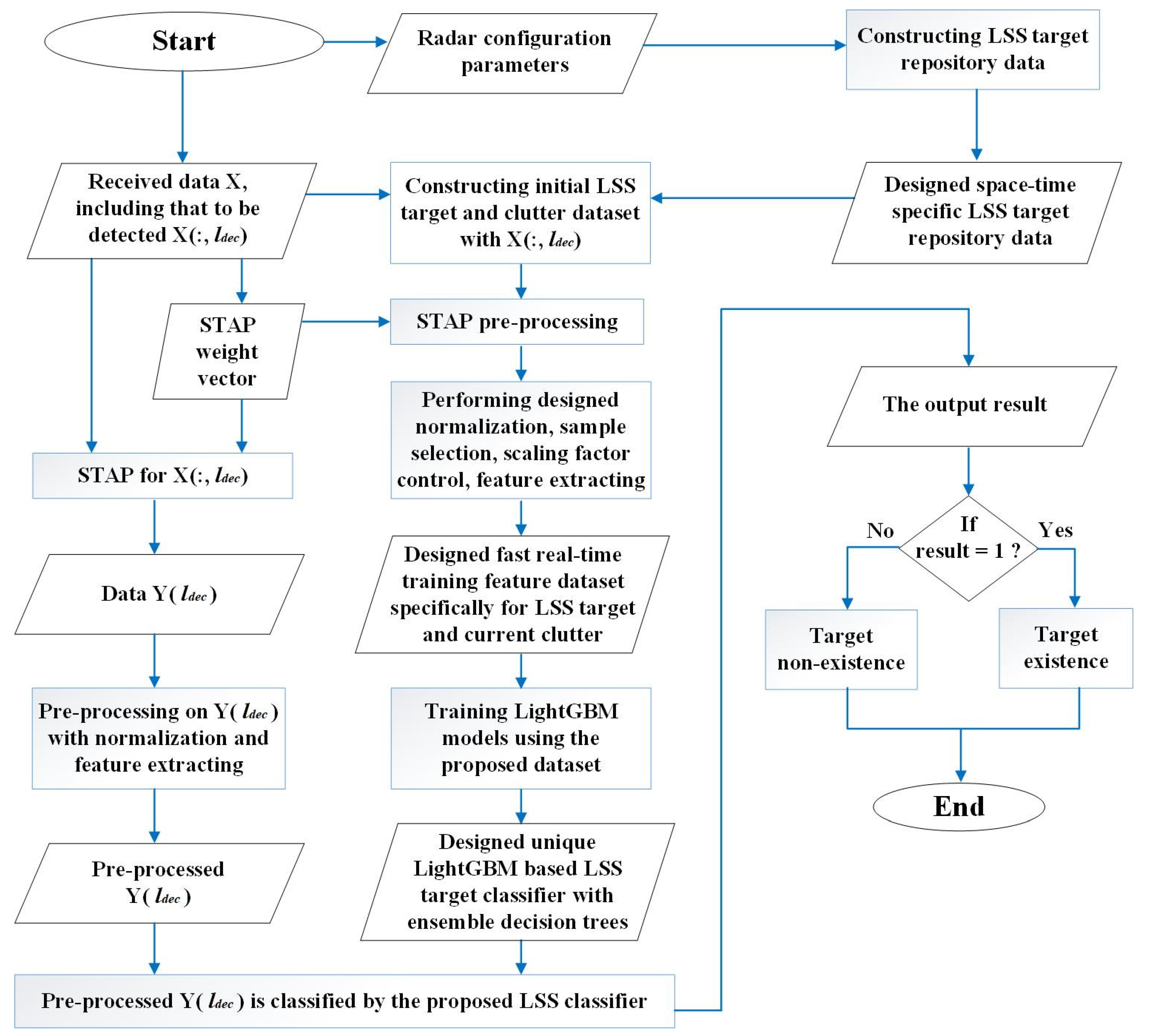
Firstly, for airborne radar, an original ensemble decision tree LightGBM-based LSS target detection framework, including the flows of data generation, data transformations, data training, and LSS target classification detection, is designed as shown in Figure 1. In this flow chart, the data that are pointed out to be designed are the main substantive innovations of the proposed method. In the following, the designed specific space–time LSS target repository data will be proposed in detail in Section 3.1; the designed fast real-time training feature dataset specifically for LSS target and current clutter will be proposed in detail in Section 3.2; the designed unique LightGBM-based LSS target classifier with ensemble decision trees will be presented in Section 3.3.
3.1. Design of Specific Space–Time LSS Target Signal Repository
To propose a targeted airborne radar detection method that is generally applicable to LSS targets, firstly, the innovative designs of a space–time two-dimensional LSS signal repository and real-time training dataset are proposed. Based on the background clutter environment of the detected cell derived from the echo data in Equations (1) and (2), a new data matrix mainly containing LSS targets is preliminarily constructed as
where and contain the LSS target and general target echoes with clutter, respectively. and represent the total numbers of targets constructed in these echoes belonging to two different classes. Specifically, and are designed as
where is the constructed -th LSS target signal. Simultaneously, in order for the proposed algorithm to detect various targets more widely, such as targets with relatively higher SNR and faster speed, non-LSS ordinary targets for are added; represents the -th non-LSS target echo. Furthermore, are the SNR, velocity, and altitude corresponding to the target, respectively. For the LSS situations of the target, the proposed method is set to
which indicates that its main component is the LSS targets with special LSS characteristics. The signal repository can be preliminarily represented as
where varies with , especially in specific detection tasks or environments. To detect a certain class or several specific targets, more targeted LSS datasets can be constructed. For different targets, to improve the characteristics of this type of LSS target, the proposed method constructs a dedicated LSS database by changing . Importantly, in Equations (11) and (13), the proposed algorithm designs and as
where and mainly embody signals with universality under different LSS conditions when changes. and are the lower and upper limits of the SNR, speed, and height that are of interest to a certain type of LSS target; similarly, and are those for the extended general targets. In addition, the complex value matches the -th target constructed in the signal repository, which is determined by the target scattering characteristics containing the SNR and target height. The impact of and on the LSS target features and radar detection results can be uniformly expressed as the reduction of the SNR.
For Equation (14), the differences among the elements in the designed signal repository originate from the differences in the considered LSS target situations . In the proposed algorithm, a different is constructed as
where , , and , respectively, represent the total number of LSS target SNRs designed within the corresponding upper and lower limits of interest, the number of different LSS target speeds, and the number of different LSS target heights; has been defined after Equation (14). The total number of LSS targets in the constructed signal repository satisfies
In Equation (14), owing to each element in the designed LSS signal repository being determined by different values for , in the proposed algorithm, the relationship existing in between and is designed as
where represents the rounding down operation and represents the remainder operation. Therefore, according to the designed correspondence between of the -th target and the -th , a whole for the designed LSS target signal repository can be constructed as a new matrix, as follows:
whose items are designed in Equations (10)–(17) and dimension is designed as
In Equation (14), for the -th LSS target that matches the condition , the kth item in its temporal steering vector is
for the pulse . More specifically, the azimuth velocity corresponds to the -th LSS target; and are the LSS target azimuth and elevation angles relative to the airborne radar. The rest of the definitions are given by Equation (1). In addition, the nth item of the spatial in Equation (14) is for .
For LSS targets with different scattering characteristics of the SNR, speed and height, the proposed algorithm has designed a specific LSS signal repository. Next, a real-time training dataset for LSS target detection and its machine learning classifier will be further designed, by which the proposed method can detect LSS targets with significantly improved performance at the low SNR, and can provide innovative strategies for the difficult detection of LSS targets.
3.2. Design of Real-Time Training LSS Target and Clutter Feature Dataset
Using the constructed exclusive LSS signal repository, based on the current clutter environment, the proposed algorithm further designs an LSS target and clutter training dataset that can be created and trained in real time. With in Equation (7) and its inverse , fully mining the space–time features and the weight vector in Equation (8), firstly, the proposed algorithm constructs the following data
where is the clutter data excluding the target cell. Another piece of data is designed as
where and are obtained by Equations (14)–(20); in addition, is
Then, based on and , mining different correspondences, the proposed algorithm designs a new data vector as
whose ith element is specifically designed as
where and have been explained after Equation (17). Consequently, the mth vector block of can be constructed as
where and is the mth element of in Equation (22). In order to facilitate the follow-up construction of the real-time LSS target and clutter training dataset, and to successfully classify and detect them, unifying the numerical standards of the dataset and making the dataset more universal are presented by the proposed algorithm. It performs standard normalization on the designed data and returns its standard score. Each item in is processed as
for , and represents the tth element of the processed in ; and are, respectively, the mean and standard deviation relevant to the mth vector block . Meanwhile, the proposed method defines and as
and
Therefore, using designed from Equations (21)–(29) and letting and , constructed in Equation (24) can be transformed into a new data matrix , as follows:
where . It deserves pointing out that the proposed algorithm does not perform the same processing on all elements in the new data , but performs different processing times on different vector blocks . Therefore, based on the current clutter environment corresponding to and , the proposed algorithm constructs and greatly expands the LSS target and clutter training dataset, providing the possibility for successful classification and detection of LSS targets.
Consequently, based on the LSS signal repository designed from Equations (10)–(20) and the new data designed from Equations (21)–(30), along with a series of matrix transformation and data processing, the proposed algorithm integrates all data and further constructs the target class dataset and the clutter class dataset separately. Specifically, the vector formed by the target class dataset is designed as
where represents the tth element of the mth vector block in . Then, employing the remaining data in the new data , the proposed method establishes the clutter class as
where , and
For , there are far more clutter data than target data, which may be imbalanced, resulting in a negative impact on the proposed detection process. In the training of the LSS target and clutter classification models, negative samples far exceeding positive ones more easily lead to adverse effects such as overfitting, slower convergence, and decreased classification performance. For radar detection, especially in low SNR situations, the intersection between the clutter and target datasets occurs. This is also the reason why it is difficult to distinguish LSS targets from clutter at a low SNR, leading to more serious false alarms. Aiming at ensuring a low false alarm probability (PFA), and simultaneous outstanding LSS detection performance, a new clutter dataset with purposeful and selective undersampling processing is designed by the proposed method. Firstly, the clutter class data are sorted into different sections as
where represents the ascending order of absolute values for the items in the clutter class ; , , and correspond to the low value, medium value, and high value parts of , respectively. Thus, the proposed method uniformly undersamples and to form new clutter dataset, as follows
where represents two uniform undersampling, and due to the relatively small proportion of , undersampling processing is omitted. However, when detecting LSS targets, in order to further effectively control the PFA, a scaling parameter factor p for the overall features of clutter class is designed by the proposed method as
Therefore, the proposed algorithm controls the PFA through this scaling factor, which can appropriately increase the data magnitude of background clutter as required. This operation restructures the clutter class dataset in terms of feature values, avoiding the aliasing of training data for the clutter and the LSS target at a low SNR.
As a result, let represent the element number of after undersampling. Combining the target class in Equation (31) and the clutter class in Equations (32)–(36), the total dataset designed and to be trained by the proposed algorithm is
where the corresponding data point label for the target class regarding to LSS signals is 1, with a number of . The data point label corresponding to the clutter class is 0, with a number of , that is
where represents the ith item of in Equation (37) and represents its label. However, to improve the training of further designed LSS target detection classifiers, the proposed algorithm extracts the features of the data points and constructs a feature vector for each data point, as follows:
where , , , and represent taking the real part, imaginary part, modulus, and phase for complex values, respectively. Let contain the feature vectors of all data points. Hence, taking into consideration the current clutter environment, the proposed algorithm designs a new real-time training feature dataset specifically for LSS targets and clutter as
where , attained from Equations (10)–(39), represents the feature vector corresponding to the ith point in and represents the corresponding label; label is clutter, while label is the target; moreover, refers to the number of items in the designed LSS target and clutter data in the given Equation (37).
3.3. Construction of LightGBM-Based LSS Target Detection Classifier with Decision Trees and Ensemble Learning
After constructing the specific space–time LSS target repository, as well as the current clutter-based fast-built real-time LSS target and clutter training feature dataset, the proposed method further constructs LSS-feature-based LightGBM training for realizing fast and outstanding LSS target detection.
LightGBM mainly involves histogram box splitting and leverages gradient single-side sampling (GOSS). It maintains fast and good classification. Moreover, the proposed LightGBM-based LSS target detection classifier requires less training data and is more adaptable to the insufficient sample size in airborne radar.
Fully exploring the designed real-time training dataset in Equation (40), that is the training dataset , the total number of vector samples is , and the corresponding label vector is . The LightGBM technique establishes a new decision tree model, on the gradient of residual reduction in each round. The decision tree model divides the data at each node, and it focuses on the feature with the maximum information gain, which is evaluated by the variance after segmentation.
Firstly, the data are boxed along the feature dimensions. When searching for the optimal segmentation point in the decision tree of the designed LSS target classifier model, the number of splits is reduced, thereby reducing the iterations and accelerating the calculation speed. Before inputting the model, is processed separately according to the columns where different features are located, that is
where represents the jth column, represents the processing by column bins, and is the jth element of in Equation (39). In addition, represents the unboxing results of all data points for the jth feature, where is the number of boxes to be divided. The sub-box processing obtains the numerical range of each feature; sets the unit bin size; obtains the numerical range for each bin; and divides the data point into the corresponding bin. Simultaneously, the histogram stores the sum of the number of samples and gradients in each sub-box.
In addition, before constructing each decision tree, the GOSS method only uses the larger gradient data and a portion of the smaller gradient data from each sub-box data to estimate the information gain, accelerating the computational efficiency and speed by changing the amount of data. It arranges the derivatives of all sample data in descending order before fitting the residuals. As a consequence, before constructing the decision tree, the total number of data in each sub-box changes, represented as with its labels .
Then, the classification task in LightGBM is viewed as an additive model that linearly combines multiple basis functions, that is
where is the basis function, which is the known scoring function based on the branching rules of the decision tree under the given data-independent variable , i.e., the weight scores of different nodes on the tree; Q is the total number of iterations and also the number of decision trees. Introducing forward step-by-step algorithm, initialize the model as
where any constant is the initial value of all samples, and if the loss function is the variance difference, then can be used to calculate the initial sample gradient . The result of the qth iteration is represented as the following model
where represents its step size. In addition, the learning rate can be introduced to escape overfitting, that is
where is the current iteration process model, and the step size in the next iteration is determined by the risk-minimization method. Specifically, by defining the loss function , the difference between the actual labels and the predicted outcomes is measured as
where, combining with the specific loss function, in the qth iteration, the loss information of each sample point is
where is the output result of the decision tree model; is the expected result; is the weight scoring basis function.
Each iteration of training generates a new tree model, reducing the residual left by the previous training. Through steepest gradient descent, minimizing the loss function whose negative gradient is the residual for fitting is introduced in LightGBM. In the qth decision tree, is
The above is the iterative process of the LightGBM integrated addition model. When the internal decision tree grows and splits, it utilizes leafwise growth. Furthermore, for each time to split, it finds the data point with the highest split information gain from all current nodes.
Specifically, let the training dataset for LSS targets on a node of the decision tree in the leafwise strategy be O, which is represented in the form of the histogram. The estimated variance gain of the histogram box point d at feature j on this node is
where is the gradient of the ith data. and represent the data points on the left and right sides of point d that belong to the subset of large gradient samples, respectively. Likewise, and represent the ones belonging to the small gradient sample subset ; represents the number of samples to the left of point d, while represents the number of samples to the right of point d; represents the total sample number; is the jth feature of the ith data ; is used to restore the data consistency. If the box point d has the maximum estimated variance gain based on the feature j, then the data points of its right and left sides are, respectively, assigned to sub-nodes of O on the corresponding side. Through these processes, the computational workload is significantly reduced without compromising training accuracy.
Therefore, for the designed LSS target real-time training dataset , performing LightGBM training, which includes the main process mentioned above, we can obtain the proposed LSS target classifier model. Finally, the proposed algorithm processes and then classifies the data from the cell to detect the LSS target, as follows:
where is the trained LSS target classification task model shown in Equation (42) and . In addition, and with . Therefore, if the data processed by and in the cell pass through the proposed LSS target classifier and the output is 1, this indicates the existence of LSS targets. On the contrary, if the output is 0, the proposed algorithm determines that there are no LSS targets. The main procedures are concluded in Algorithm 1 to summarize the proposed LightGBM-based LSS target detection algorithm.
Algorithm 1 The proposed LightGBM-based LSS target detection algorithm.
The airborne radar receives the data X as Equations (1) and (2).
According to the current real-time clutter environment of the range cell , a specific real-time space–time LSS target signal repository with special dimensions and structures is constructed:
(a)
Aiming at the LSS target characteristics, the differences in the considered LSS target situations are designed in Equations (15)–(17);
(b)
The specific space–time LSS target data and the other target data are created as Equation (14), with calculated from Equation (20);
(c)
The specific target signal repository can be constructed as Equations (17)–(19), and based on the current clutter, the target and clutter repository can be found in Equations (10)–(13).
Based on the constructed LSS target repository, a new fast-built real-time training feature dataset specifically for LSS target and current clutter, together with a series of unique data and feature transformations and processing, is designed:
(a)
Weight vector is obtained as Equation (8), with the covariance matrix estimated from Equation (7);
(b)
The weights are performed on the designed LSS signal repository and with the current clutter in the cell as Equations (21)–(23);
(c)
Normalization for each vector block is created as Equations (24)–(29) to obtain ;
(d)
The proposed method establishes the target class data and the clutter class in Equations (31)–(33);
(e)
By sorting data into blocks and selectively undersampling their processing parts, sample selection is performed as Equations (34) and (35) to obtain . Then, the scaling parameter factor p is designed to reconstruct the clutter class data and obtain the new clutter dataset in Equation (36);
(f)
By extracting features separately, the real-time training feature dataset specifically for LSS targets and clutter is formed from Equations (37)–(40).
Exploiting the designed real-time LSS target and current training feature dataset, a unique LightGBM-based LSS target detection classifier with decision trees and ensemble learning is proposed:
(a)
Histogram box splitting is implemented, forming arranged data with new features as Equation (41);
(b)
On the basis of GOSS, the variance gain is estimated and the decision trees grow in the leafwise strategy, as described in Equation (49);
(c)
The gradient of is calculated, and the residual for fitting is obtained based on Equations (47) and (48);
(d)
The decision tree model is updated for this iteration based on the addition model, and the prediction result is gained, through Equations (42)–(49);
(e)
Continue training unless the prerequisites for iteration are met. If the maximum number of iterations reaches, end the training, and obtain the proposed LightGBM-based LSS target detection classifier model.
The pre-processed data in the interested cell are classified through the proposed LSS target detection classifier.
The output results of the designed classifier for are evaluated as Equation (50), and the proposed algorithm accomplishes the LSS target detection.
For the summary of the innovations in the implementation of the proposed algorithm, the substantive innovations are mainly as follows:
(1)
Constructing an ensemble decision tree LightGBM-based LSS target detection framework, including data generation, data training, and classification detection for airborne radar, as shown in Figure 1;
(2)
Designing the space–time LSS target signal repository data and initial dataset using the current clutter data of the range cell to be detected and simultaneously taking full consideration of the low SCR and low speed of LSS targets (mainly involving substantive innovations in Equations (11), (14), (15) and (17));
(3)
Designing a series of data transformations, including signal repository data reconstruction (Equations (22) and (23)), normalization using both target and clutter data (Equations (27)–(29)), the initial formation of class datasets (Equations (31)–(33)), sample selection with block sorting and selectively undersampling (Equations (34) and (35)), scaling parameter factor transformation (Equation (36)), and extracting features (Equation (39)), to construct real-time training feature datasets specifically for LSS targets and clutter.
In addition, apart from the substantive innovations mentioned above, the proposed algorithm has conducted in-depth analysis on the designed data structures, as well as the correlation between the designed data and the LSS target features, such as Equations (24)–(26) and (30).
4. Simulation Results
In this section, the simulation outcomes and detection results with the experimental data are employed to validate the merits of the proposed algorithm. A side-looking airborne radar with = 0.03 m, d = 0.015 m, platform height = 0.015 m, and azimuth angle is considered. In the result figures, the PFA is controlled as for all analyzed algorithms apart from those with special PFA descriptions. As a widely used performance evaluation of radar target detection, the probability of detection (PD) is brought in and defined as under the desired PFA, with being the number of successful target detections and being the total number of detection attempts. The noise power is fixed. The scattering coefficients of clutter patches are complex Gaussian distributed. The clutter-to-noise ratio (CNR) establishes the amplitudes of the clutter coefficients. Other parameters for comprehensive performance evaluations will be separately introduced.
4.1. Effectiveness Visualization of the Proposed Algorithm
Figure 2 shows the visual effects of the proposed LSS target detection algorithm, where there exists array elements, -pulses, range cells, and = 45 dB. The SNR of the LSS target is dB in Figure 2a, while Figure 2b is without targets. The height and velocity of the LSS target are and , respectively. The axes of this figure correspond to the three-dimensional feature vectors of the data points. The blue and red data points represent the LSS target and clutter in the designed real-time training feature dataset, respectively. All shown data points constitute the designed training dataset. From the visualization, the distribution of clutter and LSS target data in the designed dataset can be intuitively seen. When detecting the LSS target successfully, the LSS targets with similar feature vectors of the targets are within the desired LSS target distribution range, and located near the blue dots in the visualization diagram, as shown in Figure 2a. By contrast, when detecting the LSS target in a failed attempt, the LSS target points with similar feature vectors of clutter are within the distribution range relevant to clutter, and located near the red dots in the visualization. They demonstrate that the proposed LSS target detection algorithm is effective.
4.2. Performance Comparison of Different Methods
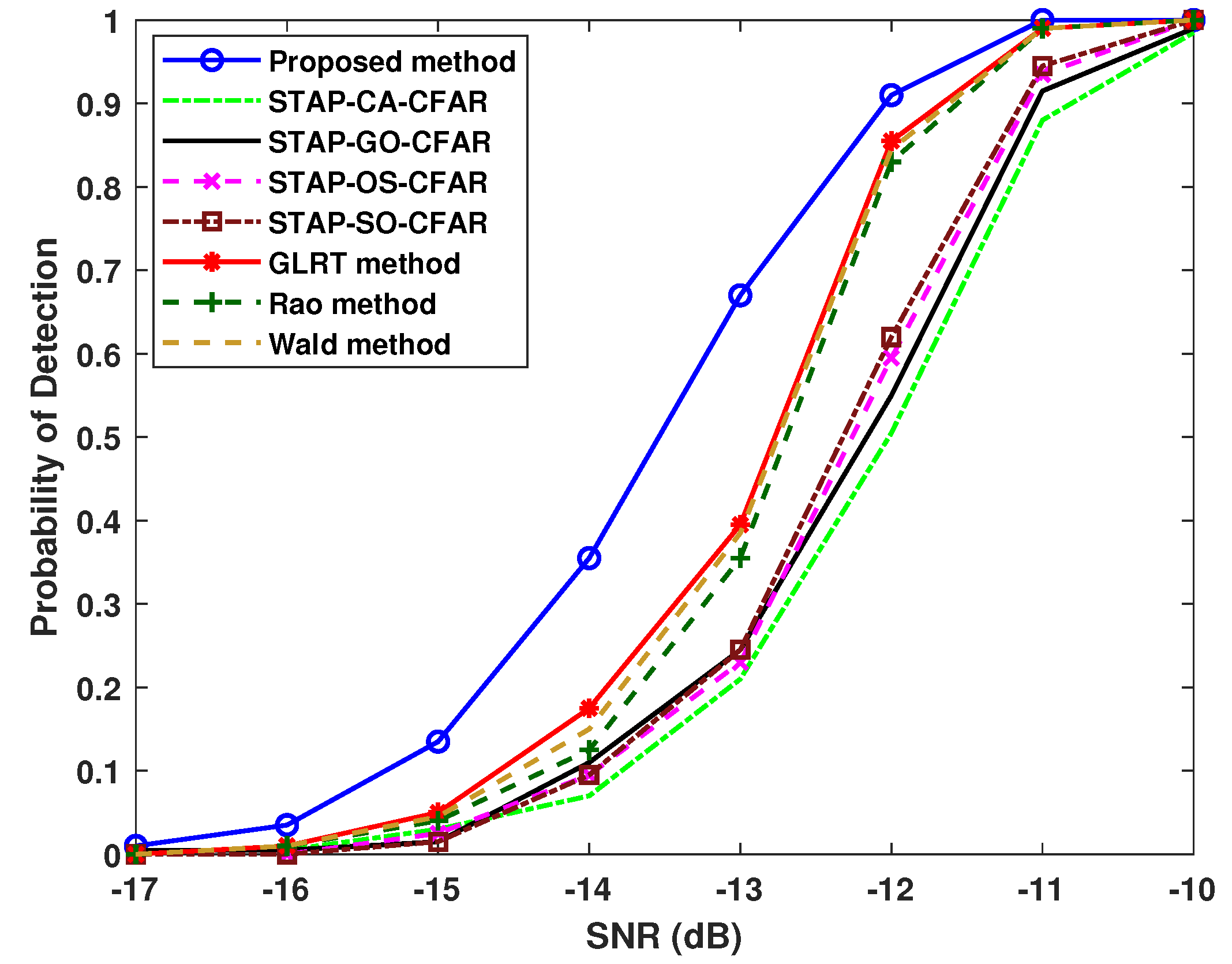
In Figure 3, the same condition is kept as Figure 2, except that and . It exhibits that the proposed algorithm for LSS targets provides significantly better LSS target detection performance than the other methods, especially under the LSS target environments with a low SNR. When , the proposed algorithm achieves detection probability, being significantly superior to the GLRT method with , and the best among these LSS target and clutter environments. Even though the other algorithms almost cannot successfully detect the LSS target at and , the proposed method still achieves some detections.
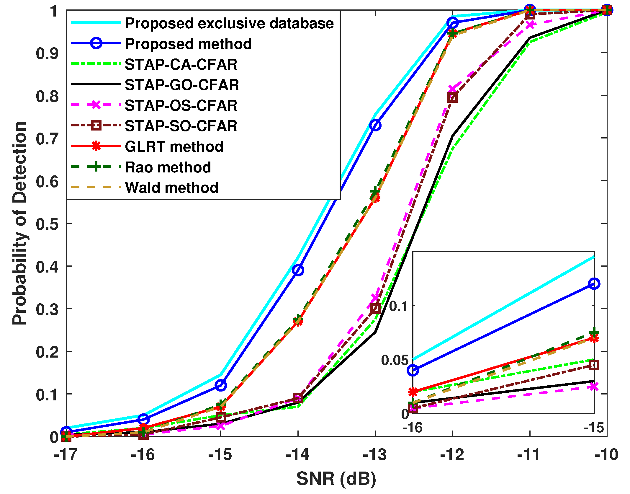
It deserves exhibiting that the proposed method can be constructed specifically and flexibly for different types of LSS targets, by designing the corresponding specific LSS target and clutter training feature dataset of interest. For example, in Figure 4, the LSS target has and . The extra specific database shown as the proposed exclusive database is constructed by the proposed method, containing the LSS targets with ∼, ∼, and ∼. Figure 4 shows that, compared to the proposed LSS database with universality used in all the figures, the specific database constructed by the proposed method in Figure 4 can further improve LSS target performance. Among the different methods, these databases of the proposed method both realize the best performance.
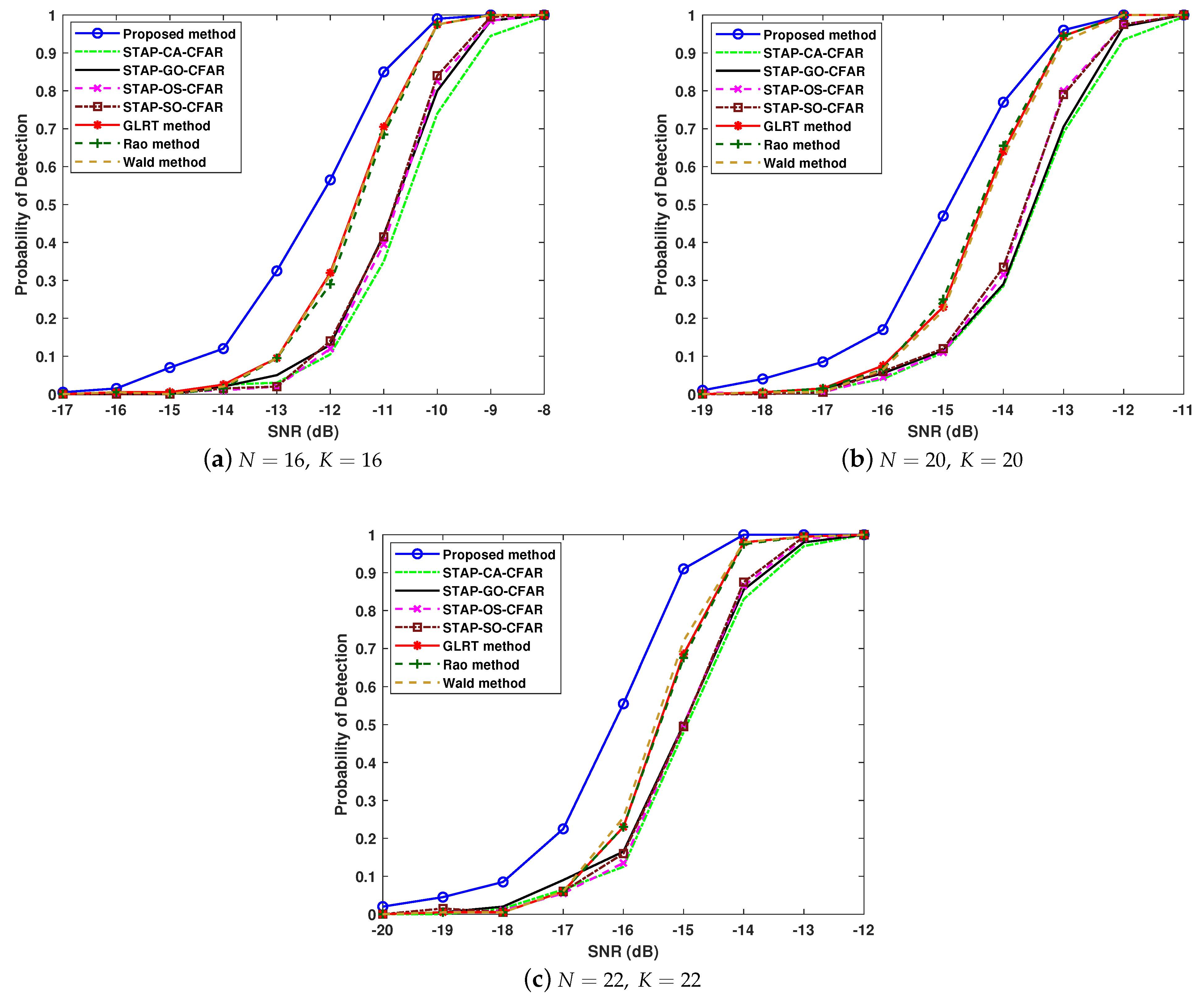
In Figure 5a–c, the radar configurations are , , and , respectively. The others are the same as Figure 4. It shows under different radar configurations that the proposed algorithm still performs better in LSS target detection with a low SNR than the others.
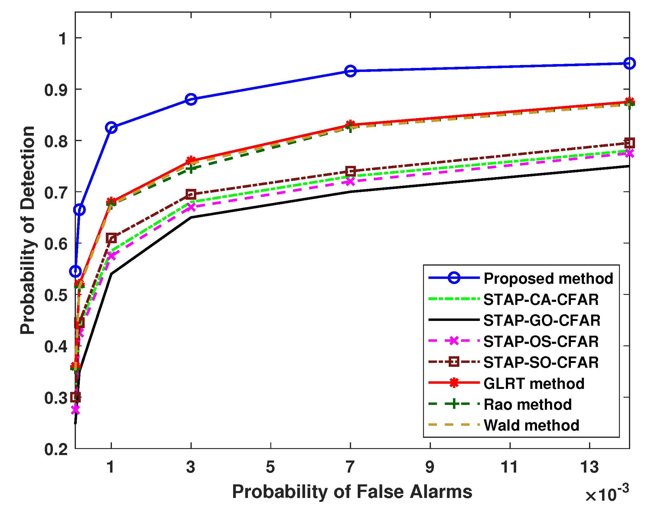
Figure 6 verifies the performance comparison under the changing PFA conditions, where , and the others align with Figure 2. Among the different methods, the proposed LSS target detector possesses the best and excellent performance, providing much higher detection probabilities.
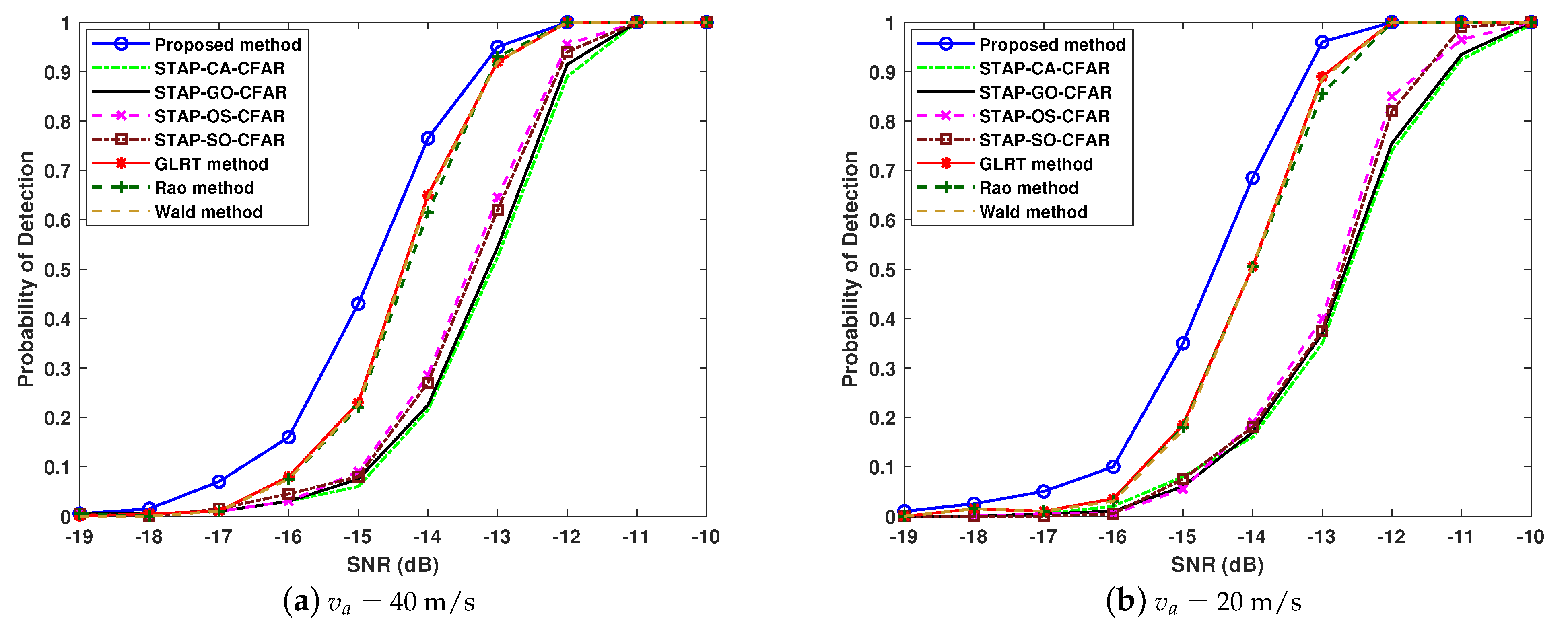
Figure 7 shows, with different LSS target velocities, the detection result comparisons. The target velocities are in Figure 7a, while in Figure 7b, referring to Figure 3 for the remaining conditions. The advantages of the proposed LSS target detector are maintained at different target velocities, demonstrating its insensitivity to the LSS target environment including the velocity.
4.3. Computation Time of Different Methods
The real-time performance and detection time of different methods are contrasted in Table 1. The main time-consuming procedure of the proposed method is creating the training dataset, while for the other algorithms, it is obtaining the inverse . Except for OS-CFAR, the other mean level class algorithms of CFAR cost similarly; therefore, they are uniformly shown as ML-CFAR. Besides, simulations are performed to generate the averaging.
From Table 1, it can be seen that, as (N, K) decreases, the difference in time between the proposed method and the other methods becomes smaller. The computation time of all methods is less than 1 s, while the proposed method only takes approximately 1.5-times that of the other traditional detection methods. For the proposed LSS detection algorithm, the time is only slightly higher, but the performance is remarkably improved, proving that the computational time of the proposed detector is deemed appropriate.
The time efficiency of relevant different ensemble decision tree techniques [25] is evaluated, for GBDT, CatBoost, XGBoost, random forest, and the proposed method. It is evident that the proposed LightGBM-based LSS target detector consumes notably less processing time than the other traditional classifiers. For example, when , only the proposed method costs less than 1 s; the computational times of the GBDT, CatBoost, XGBoost, and random forest methods are approximately 22-times, 9.9-times, 1.8-times, and 2.8-times that of the proposed method, respectively. It is worth emphasizing that the performance comparison of all methods in Table 2 corresponds to Figure 13.
4.4. Impact of Parameter Settings and Array Configuration
By changing the learning rate while referring to Figure 2 for the remaining unchanged conditions, the effect of during the update iteration processes on the proposed method is analyzed. Changing does not affect the PFA. Figure 8 verifies that, when , it causes the loss function to oscillate, leading to a deterioration of the proposed method. However, when , the convergence is too slow, and insufficient iterations also affect the detection efficiency. The optimal of the proposed LightGBM-based LSS target detector is , which promotes convergence and prevents oscillation, achieving the best performance.
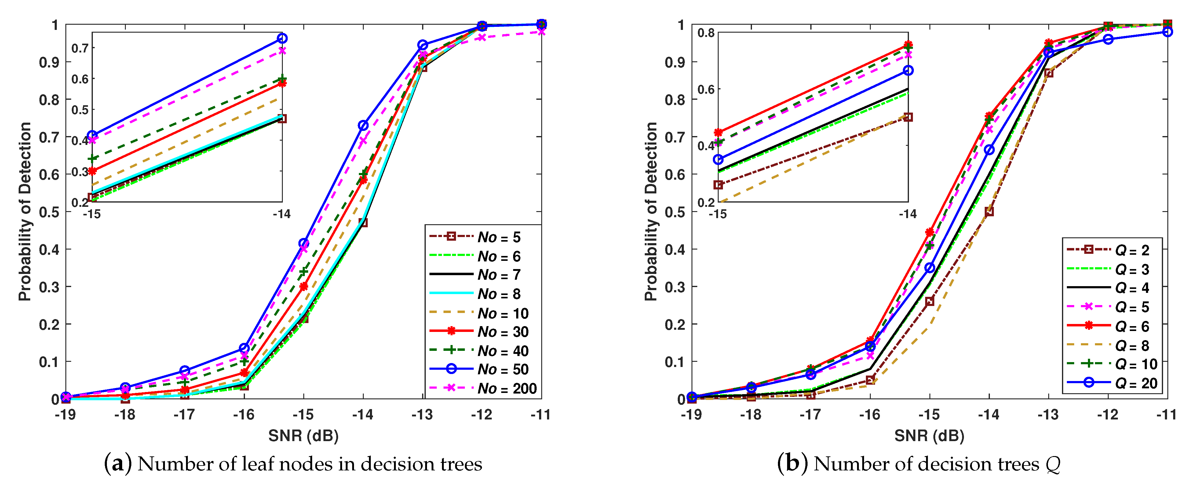
In Figure 9, the parameter effects of the ensemble decision trees on the proposed LSS target detector are analyzed. The numbers of decision trees and leaf nodes are considered. The conditions refer to Figure 2, except for the varied parameters; Q and are evaluated separately in Figure 9a,b. With increased , the proposed LSS target classifier training has more accuracy. However, it requires more times for the split within the same node and weakens the generalization ability by overfitting. Furthermore, Figure 9 demonstrates that is inferior to , as it overfits.
Similarly, the excessive Q also leads to overfitting. When , overfitting occurs, resulting in worsened performance. In the proposed LSS target detector with the designed real-time feature dataset, and can achieve excellent detection performance.
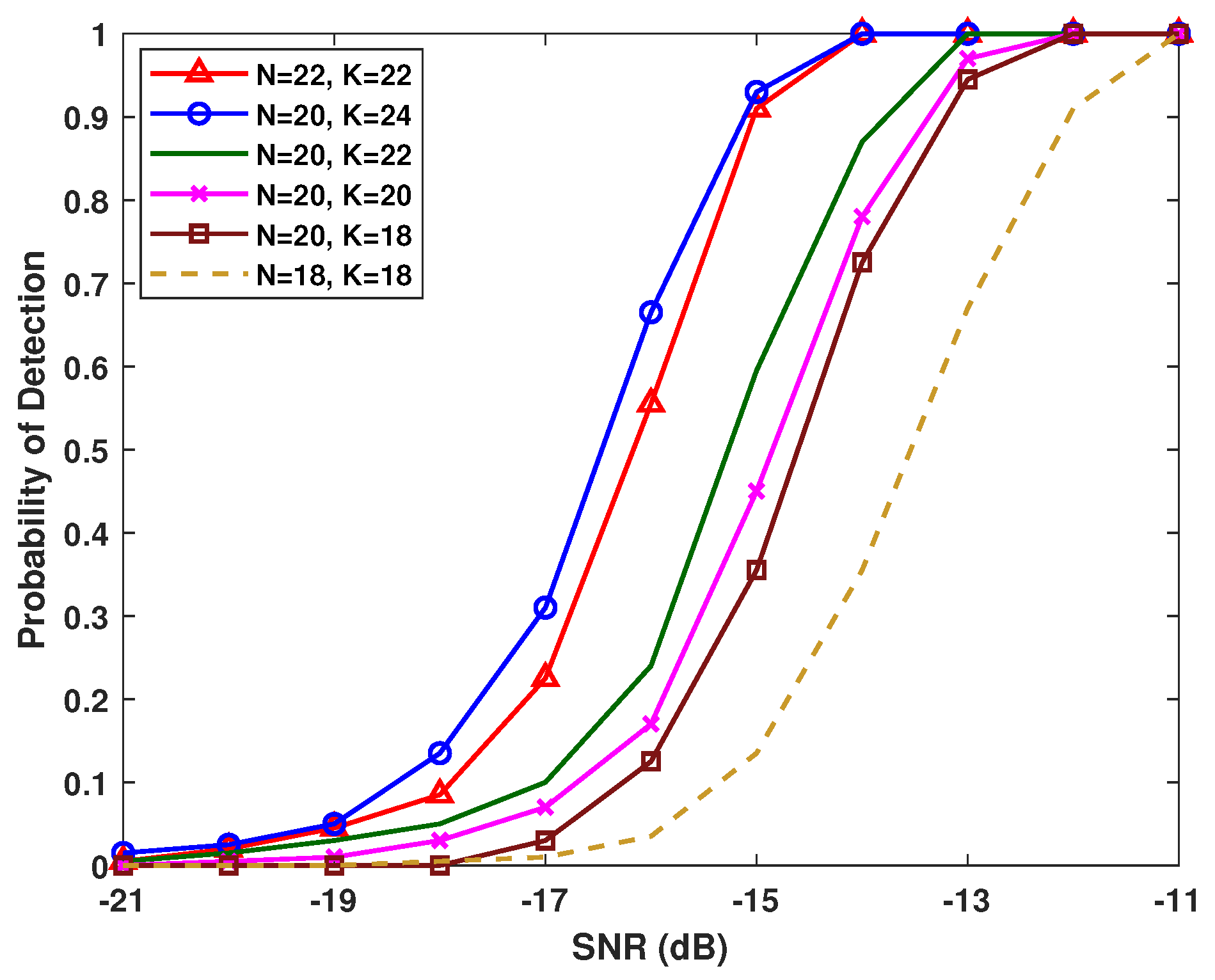
Figure 10 shows the LSS detection performance versus N and K represented for numbers of array elements and pulses, with the varying ∼22 and ∼24. As and increase, the proposed LSS target detection performance increases greatly. Although these array configurations significantly affect the desired detection, the proposed detector can remain advantageous with different N and K, as demonstrated in Figure 10.
4.5. Classification Evaluation Metrics and PFA of Proposed LSS Target Detector
Because the proposed method is based on machine learning classification, the classical classification evaluation metrics [36] that exclusively belong to machine learning classification methods are employed to evaluate the proposed LSS target detection classifier. The specific definitions of these machine learning classification metrics can be found in [36]. Unlike the traditional performance evaluation of the probability of detection used in other figures, the metrics included in Figure 11 are specific to the classic evaluation of machine learning classification, rather than direct radar detection evaluation. However, these metrics can also reflect the correctness and accuracy of the designed part of machine learning classification involved in the proposed method from another perspective.
Meanwhile, the designed scaling parameter factors p with different values are considered to show its influence on the classification. In Figure 11, the condition , and the others refer to Figure 2. It reflects that the PFA decreases with the increased p, greatly avoiding false alarms. In addition, the important metric, recall, representing the LSS detection results for both the prediction and actual objectives, increases with p. The other four famous metrics including the AUC decrease as p increases. Figure 11 proves that, when , it can detect the LSS target with the greatest possibility while ensuring the PFA, achieving the best detection performance along with machine learning classification performance.
4.6. Performance Comparison of Different Machine Learning Techniques
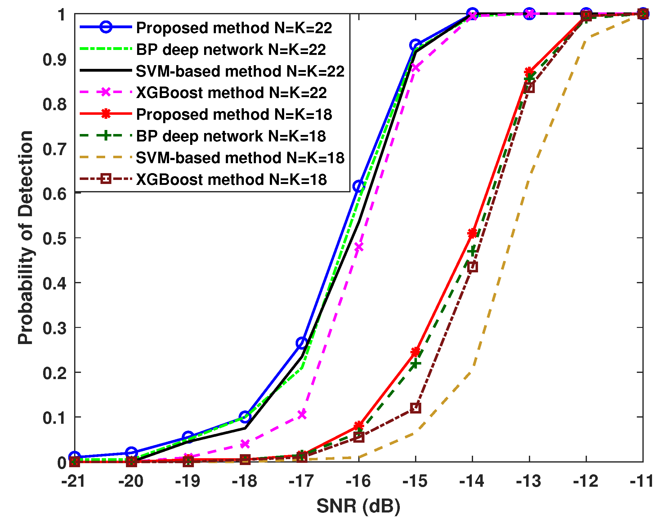
In addition to the above-mentioned classic airborne radar target detection methods for comparison, the performance comparison scope is broadened to include diverse techniques, including the deep learning method and the SVM-based method [37]. As a classic deep learning algorithm, the back propagation (BP) neural network method [38] is introduced for comparison. Moreover, in Table 2, except for the proposed method, the XGBoost method, which has the shortest processing time among the other ensemble decision tree methods, is also considered.
In Figure 12, the influence of different radar configurations on diverse techniques is considered, and the other conditions are consistent with Figure 4. Figure 12 shows that the proposed method performs better than the BP deep neural network and the SVM-based method, especially in low-SNR situations. In addition, as the radar configuration increases, the proposed method does not exhibit significant fluctuations like SVM, but consistently maintains better performance. The proposed method demonstrates advantages in different machine learning techniques including deep learning- and SVM-based methods.
In Figure 13, different ensemble decision tree algorithms, whose computation time is shown in Table 2, are evaluated for their target detection performance with the detection probability. It shows that LightGBM in the proposed method has a similar performance to the GBDT method. Furthermore, the other decision tree methods have slightly lower detection probabilities; meanwhile, their required computation time greatly increases, as shown in Table 2. The proposed LightGBM-based algorithm effectively balances detection performance and computation time, better meeting real-time requirements and practical application needs.
Figure 13.
Performance comparison of different ensemble decision tree algorithms.
Figure 13.
Performance comparison of different ensemble decision tree algorithms.
4.7. Detection Results of Different Methods with Experimental Data
Experimental data for airborne radar in a real clutter environment including ground clutter and sea clutter are used to evaluate different detection methods. The real experimental data are multi-channel airborne radar measurements (MCARMs), whose radar configuration and clutter environment are described in detail in [39]. In particular, the angle between the array and the platform moving direction is . The following experimental data are extracted from pulses together with the first sub-arrays for each range cell in the MCARM dataset.
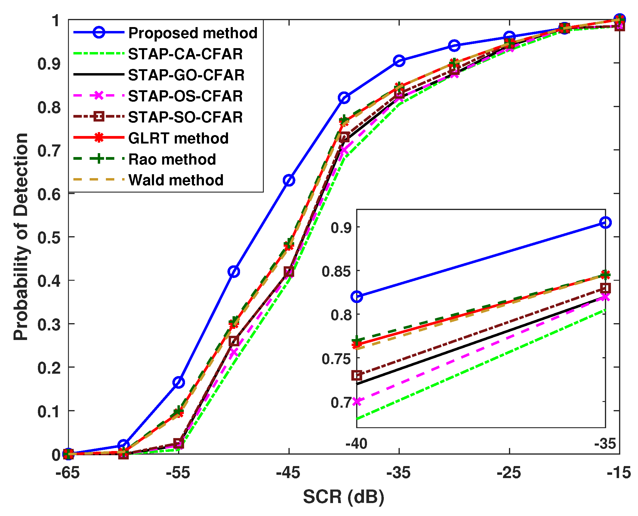
In Figure 14, the real clutter experimental data without strong targets are extracted from to range cells. Then, the target signal including the LSS target is injected into the range cell , with to . In addition, the proposed LSS target signal repository is constructed as Equations (14)–(20) with to .
Consequently, the detection results with the experimental data for different methods can be analyzed for more comprehensive performance evaluation. Figure 14 proves that the proposed LSS target detection algorithm is effective for the experimental data. Moreover, it has stable and significant advantages compared to other analyzed methods, especially in the low-SCR range.
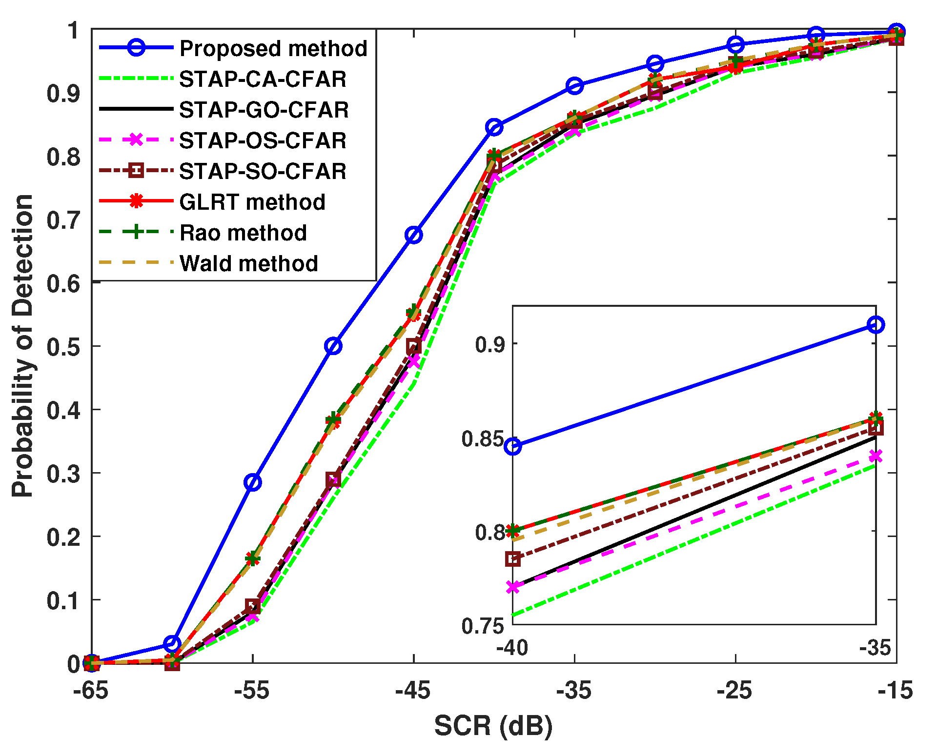
In Figure 15, the real clutter of airborne radar is from the measured data with to range cells. The target signal including the LSS target is injected into the range cell. The PFA stays the same for all the methods. Figure 15 validates the effectiveness and merits of the proposed algorithm. In effect, for this detection result, it just takes to process. Among the different methods, the best detection is accomplished by the proposed LSS target detection method within a large range of the SCR.
5. Discussion
Discussion 1: The innovation analyses of the proposed method aiming at LSS target detection and the reason for its performance merits are as follows. Firstly, the algorithm designs a space–time two-dimensional signal repository with special dimensions and structures, specifically for airborne radar LSS targets. It fully explores and utilizes the clutter environment of the current range cell under detection. It not only has good adaptability to the clutter environment, but also fully considers the LSS target features of the SNR, height, and velocity, thus enabling targeted detection for this specific class of LSS target.
Secondly, the proposed method designs a real-time training feature dataset specifically for LSS targets and clutter, along with a series of data and feature transformations and processing. Additionally, it fully explores the richer multidimensional feature information of the data phase, real part, and imaginary part, which cannot be independently utilized by traditional methods such as the CFAR-based ones. Therefore, the proposed algorithm significantly enhances the performance of LSS target detection.
Thirdly, the proposed method designs a unique machine learning-based LSS target detection classifier. It is developed by fully exploiting and utilizing the advantages of ensemble decision trees-based LightGBM technology, thereby achieving excellent classification for LSS targets and clutter. It is not sensitive to the number of samples and can adapt to environments with a small number of clutter and target samples. Additionally, its training is fast. Therefore, the proposed method greatly strengthens the LSS target features and suppresses clutter by designing a specific space–time LSS target signal repository and a fast-built real-time training feature dataset, allowing the proposed machine learning classification advantages to be fully utilized, and then achieving excellent LSS target detection.
Discussion 2: The computational complexity of the proposed LSS target detection algorithm is analyzed as follows. Constructing the LSS target signal repository and training feature dataset requires , which mainly involves obtaining the weight vector and the signal repository and , and performing on the designed repository. In addition, the development of the LightGBM-based detection classifier requires , where f, , , and Q are the numbers of features, samples after GOSS, boxes after the histogram, and the decision trees; k is the depth of the decision trees. It has high time efficiency. Hence, the computation complexity is . The proposed algorithm notably enhances the LSS target detection performance with appropriate processing time.
Discussion 3: The experience parameter that needs to be carefully adjusted when constructing the real-time training dataset is the designed scaling factor p in the Equation (36), as analyzed below. The parameter p plays a role in the overall scaling of the characteristic values of the clutter class dataset, typically ranging from to . The values of the corresponding four-dimensional clutter feature from Equations (36)–(39) increases with the growth of p. Therefore, the smaller p is, the greater the differences in the feature values between the clutter dataset and the LSS target dataset are. Hence, it will be easier to detect the LSS target after model training. However, the PFA and detection probability have the same variation pattern. Therefore, it is necessary to control this parameter reasonably in order to satisfy the PFA and simultaneously detect more targets.
In addition, the setting of p is closely related to the ratio of the target class and clutter class data in the designed training dataset, which is determined by the undersampling processing ratio for the clutter class in Equation (35). A larger p is required when the proportion of the target class data in the training dataset increases. This is because the classification model can learn more information regarding the target class, making it easier to detect LSS targets. Therefore, increasing p is necessary to control the PFA. Generally, for the proposed LSS target detector, when the data ratio of clutter to target is set to 50:1 through undersampling processing, controlling the desired PFA can be achieved by setting .
Discussion 4: During the development of the LSS target LightGBM classification model, the proposed approach requires specific adjustments to the numbers of leaf nodes, decision trees, and the learning rate, that is , Q, and . Increasing each of the first two parameters separately enhances the detection capability of the proposed algorithm. However, excessively large values not only cost more training time, but also lead to overfitting, ultimately decreasing the generalization ability of classification and the target detection capability of the proposed LSS target detector. Moreover, the learning rate multiplied before the step size to prevent the overfitting should also be considered to balance the convergence and the real-time performance. Generally, in the proposed algorithm is supportive of attaining great performance and fast speed.
6. Conclusions
In this paper, a novel LightGBM-based low–slow–small target detection algorithm for airborne radar is proposed. In the proposed algorithm, after constructing the specific space–time LSS target signal repository with special dimensions and structures, the new fast-built real-time training feature dataset specifically for LSS targets and clutter, together with a series of unique data and feature transformations and processing, is designed. Then, by proposing a unique machine learning-based LSS target detection classifier employing the advantages of decision trees and ensemble learning-based LightGBM, the pre-processed data in the range cell of interest are classified and the classifier output result is evaluated, to achieve the LSS target detection. The factors contributing to the performance merits and to the appropriate computational time of the proposed LSS target detection algorithm are analyzed. Besides, the experience parameters involved are discussed in detail. The simulation outcomes and detection results with experimental data verify that the proposed algorithm is effective and possesses stable and obvious advantages of target detection, especially at the low SCR for LSS targets. Furthermore, the proposed algorithm accomplishes significantly superior target detection with much higher detection probabilities.
Author Contributions
Conceptualization, J.L.; methodology, J.L.; software, J.L. and P.H.; formal analysis, J.L. and C.Z.; resources, J.L.; writing—original draft preparation, J.L. and P.H.; writing—review and editing, J.L., F.H.J. and G.L.; project administration, J.L., C.Z., H.T. and J.X.; funding acquisition, J.L., C.Z., G.L. and H.T.; supervision, J.L., G.L., J.X., F.H.J. and H.T. All authors have read and agreed to the published version of the manuscript.
Funding
This work was supported by the stabilization support of the National Radar Signal Processing Laboratory under Grant KGJ20230X and the NSFC under Grants 61931016 and 62071344.
Klemm, R. Principles of Space-Time Adaptive Processing; The Institution of Electrical Engineers: London, UK, 2002. [Google Scholar]
Brown, R.D.; Schneible, R.A.; Wicks, M.C.; Wang, H.; Zhang, Y.H. STAP for clutter suppression with sum and difference beams. IEEE Trans. Aerosp. Electron. Syst.2000, 36, 634–646. [Google Scholar] [CrossRef]
Wang, Y.; Peng, Y. Space-time joint processing method for simultaneous clutter and jamming rejection in airborne radar. Electron. Lett.1996, 32, 258. [Google Scholar] [CrossRef]
Dipietro, R.C. Extended factored space-time processing for airborne radar systems. In Proceedings of the 26th Asilomar Conference, Pacific Grove, CA, USA, 26–28 October 1992; pp. 425–430. [Google Scholar]
Liu, J.; Liao, G.S.; Xu, J.W.; Zhu, S.Q.; Juwono, F.J.; Zeng, C. Autoencoder neural network-based STAP algorithm for airborne radar with inadequate training samples. Remote Sens.2022, 14, 6021. [Google Scholar] [CrossRef]
Cotter, S.F.; Rao, B.D.; Engan, K.; Delgado, K.K. Sparse solutions to linear inverseproblems with multiple measurement vectors. IEEE Trans. Signal Process.2005, 53, 2477–2488. [Google Scholar] [CrossRef]
Han, S.D.; Fan, C.Y.; Huang, X.T. A novel STAP based on spectrum-aided reduced-dimension clutter sparse recovery. IEEE Geosci. Remote Sens. Lett.2017, 14, 213–217. [Google Scholar] [CrossRef]
Ji, S.; Xue, Y.; Carin, L. Bayesian compressive sensing. IEEE Trans. Signal Process.2008, 56, 2346–2356. [Google Scholar] [CrossRef]
Feng, W.K.; Guo, Y.D.; Zhang, Y.S.; Gong, J. Airborne radar space time adaptive processing based on atomic norm minimization. Signal Process.2018, 148, 31–40. [Google Scholar] [CrossRef]
Yang, Z.C.; de Lamare, R.C.; Li, X. L1-regularized STAP algorithms with a generalized sidelobe canceler architecture for airborne radar. IEEE Trans. Signal Process.2011, 60, 674–686. [Google Scholar] [CrossRef]
Maria, S.; Fuchs, J.J. Detection performance for the GMF applied to STAP data. In Proceedings of the 2006 14th European Signal Processing Conference, Florence, Italy, 4–8 September 2006; pp. 1–5. [Google Scholar]
Ma, Z.; Liu, Y.; Meng, H.; Wang, X. Jointly sparse recovery of multiple snapshots in STAP. In Proceedings of the 2013 IEEE Radar Conference (RadarCon13), Ottawa, ON, Canada, 29 April–3 May 2013; pp. 1–4. [Google Scholar]
Finn, H.M. Adaptive detection mode with threshold control as a function of spatially sampled clutter-level estimates. RCA Rev.1968, 29, 414–465. [Google Scholar]
Trunk, G.V. Range resolution of targets using automatic detectors. IEEE Trans. AES1978, 14, 750–755. [Google Scholar] [CrossRef]
Hansen, V.G. Constant false alarm rate processing in search radars. In Proceedings of the IEEE International Radar Conference, IEEE Radar Present and Future, London, UK, 23–25 October 1973; pp. 322–325. [Google Scholar]
Rohling, H. Radar CFAR thresholding in clutter and multiple target situations. IEEE Trans. Aerosp. Electron. Syst.1983, 19, 608–621. [Google Scholar] [CrossRef]
De, M.A. Rao test for adaptive detection in Gaussian interference with unknown covariance matrix. IEEE Trans. Signal Process.2007, 55, 3577–3584. [Google Scholar]
Conte, E.; De, M.A.; Galdi, C. Statistical analysis of real clutter at different range resolutions. IEEE Trans. Aerosp. Electron.2004, 40, 903–918. [Google Scholar] [CrossRef]
Ball, J.E. Low signal-to-noise ratio radar target detection using Linear Support Vector Machines (L-SVM). In Proceedings of the 2014 IEEE Radar Conference, Cincinnati, OH, USA, 19–23 May 2014; pp. 1291–1294. [Google Scholar]
Xia, X.; Leung, H. Nonlinear Spatial-temporal Prediction Based on Optimal Fusion. IEEE Trans. Neural Netw.2006, 17, 975–988. [Google Scholar] [CrossRef]
Chai, B.; Chen, L.; Shi, H.; He, C. Marine ship detection method for SAR image based on improved faster RCNN. In Proceedings of the 2021 SAR in Big Data Era (BIGSARDATA), Nanjing, China, 22–24 September 2021; pp. 1–4. [Google Scholar]
Zhang, Z.; Wu, D.; Zhu, D.; Zhang, Y. A multichannel SAR ground moving target detection algorithm based on subdomain adaptive residual network. IEEE Geosci. Remote Sens. Lett.2023, 20, 1–5. [Google Scholar] [CrossRef]
Wang, S.; Li, J.; Wang, Y.; Li, Y. Radar HRRP target recognition based on Gradient Boosting Decision Tree. In Proceedings of the 2016 9th International Congress on Image and Signal Processing, BioMedical Engineering and Informatics (CISP-BMEI), Datong, China, 15–17 October 2016; pp. 1013–1017. [Google Scholar]
Jiang, Y.; Cheng, D.; Qi, W.; Song, R.; Yu, C.; Liu, S. Radar target recognition of individuals based on XGBoost. In Proceedings of the 2023 IEEE 3rd International Conference on Information Technology, Big Data and Artificial Intelligence (ICIBA), Chongqing, China, 26–28 May 2023; pp. 1110–1113. [Google Scholar]
Guan, S.; Gao, X.; Lang, P.; Dong, J. The corner reflector array recognition based on multi-domain features extraction and CatBoost. In Proceedings of the 2023 8th International Conference on Intelligent Computing and Signal Processing (ICSP), Xi’an, China, 21–23 April 2023; pp. 1725–1730. [Google Scholar]
Ham, J.; Chen, Y.C.; Crawford, M.M.; Ghosh, J. Investigation of the random forest framework for classification of hyperspectral data. IEEE Geosci. Remote Sens.2005, 43, 492–501. [Google Scholar] [CrossRef]
Cai, L.; Qian, H.; Xing, L.; Zou, Y.; Qiu, L.; Liu, Z.; Tian, S.; Li, H. A Software-Defined Radar for Low-Altitude Slow-Moving Small Targets Detection Using Transmit Beam Control. Remote Sens.2023, 15, 3371. [Google Scholar] [CrossRef]
Yu, J.; Liu, Y.l.; Bai, Y.; Liu, F.l. A double-threshold target detection method in detecting low slow small target. Proc. Comput. Sci.2020, 174, 616–624. [Google Scholar] [CrossRef]
Shi, S.N.; Liang, X.; Shui, P.L.; Zhang, J.K.; Zhang, S. Low-velocity small target detection with Doppler-guided retrospective filter in high-resolution radar at fast scan mode. IEEE Geosci. Remote Sens.2019, 57, 8937–8953. [Google Scholar] [CrossRef]
Guo, K.; Zheng, X.; Shi, S.; Qin, K.; Xie, T. A low-slow-small target detection method for offshore radar based on GPU. In Proceedings of the 2021 2nd China International SAR Symposium (CISS), Shanghai, China, 3–5 November 2021; pp. 1–4. [Google Scholar]
Musa, S.A.; Abdullah, R.S.; Sali, A.; Ismail, A.; Abdul Rashid, N.E. Low-slow-small (LSS) target detection based on micro Doppler analysis in forward scattering radar geometry. Sensors2019, 19, 3332. [Google Scholar] [CrossRef] [PubMed]
Novakovic, J.; Veljovic, A.; Ilic, S.; Papic, T. Evaluation of classification models in machine learning. Theory Appl. Math. Comput. Sci.2017, 7, 39–46. [Google Scholar]
Sarkar, T.K.; Wang, H.; Park, S.; Adve, R.; Koh, J.; Kim, K.; Zhang, Y.H.; Wicks, M.C.; Brown, R.D. A deterministic least-squares approach to space-time adaptive processing. IEEE Trans. Antennas Propag.2001, 49, 91–103. [Google Scholar] [CrossRef]
Figure 1.
Designed ensemble decision tree LightGBM-based LSS target detection framework.
Figure 1.
Designed ensemble decision tree LightGBM-based LSS target detection framework.
Figure 2.
Visualization of the proposed LSS target detection classifier.
Figure 2.
Visualization of the proposed LSS target detection classifier.
Figure 3.
Detection probabilities of different methods.
Figure 3.
Detection probabilities of different methods.
Figure 4.
Detection probabilities of different methods and constructed exclusive signal repository.
Figure 4.
Detection probabilities of different methods and constructed exclusive signal repository.
Figure 5.
Detection probabilities of different methods with different radar configurations.
Figure 5.
Detection probabilities of different methods with different radar configurations.
Figure 6.
Performance of different methods versus the PFA.
Figure 6.
Performance of different methods versus the PFA.
Figure 7.
Performance of different methods versus LSS target speed.
Figure 7.
Performance of different methods versus LSS target speed.
Figure 8.
Impact of learning rate on LSS target detection performance.
Figure 8.
Impact of learning rate on LSS target detection performance.
Figure 9.
Impact of ensemble decision tree parameters on LSS target detection performance.
Figure 9.
Impact of ensemble decision tree parameters on LSS target detection performance.
Figure 10.
Impact of radar configurations N and K on the proposed LSS target detection method.
Figure 10.
Impact of radar configurations N and K on the proposed LSS target detection method.
Figure 11.
Classification evaluation metrics and the PFA versus scaling parameter factor p.
Figure 11.
Classification evaluation metrics and the PFA versus scaling parameter factor p.
Figure 12.
Performance comparison of different machine learning methods.
Figure 12.
Performance comparison of different machine learning methods.
Figure 14.
Detection performance with experimental data.
Figure 14.
Detection performance with experimental data.
Figure 15.
Detection performance with different experimental data.
Figure 15.
Detection performance with different experimental data.
Table 1.
Computation time of different detection algorithms.
Table 1.
Computation time of different detection algorithms.
(N,K)
Average Computation Time
Proposed Method
GLRT
Rao
Wald
ML-CFAR
OS-CFAR
(14,14)
0.580 s
0.398 s
0.368 s
0.363 s
0.383 s
0.370 s
(16,16)
0.676 s
0.465 s
0.428 s
0.423 s
0.446 s
0.489 s
(18,18)
0.778 s
0.553 s
0.531 s
0.529 s
0.521 s
0.534 s
(20,20)
0.931 s
0.64 s
0.59 s
0.582 s
0.585 s
0.594 s
Table 2.
Computation time of different ensemble decision tree algorithms.
Table 2.
Computation time of different ensemble decision tree algorithms.
(N,K)
Average Computation Time
Proposed Method
GBDT
CatBoost
XGBoost
Random Forest
(14,14)
0.580 s
12.766 s
5.763 s
1.075 s
1.634 s
(16,16)
0.676 s
12.862 s
5.859 s
1.171 s
1.751 s
(18,18)
0.778 s
13.576 s
5.961 s
1.273 s
1.853 s
(20,20)
0.931 s
13.727 s
6.112 s
1.424 s
2.004 s
(22,22)
1.186 s
13.984 s
6.369 s
1.681 s
2.261 s
Disclaimer/Publisher’s Note: The statements, opinions and data contained in all publications are solely those of the individual author(s) and contributor(s) and not of MDPI and/or the editor(s). MDPI and/or the editor(s) disclaim responsibility for any injury to people or property resulting from any ideas, methods, instructions or products referred to in the content.


 ,
, 


