Article

Aerosol Optical Properties Retrieved by Polarization Raman Lidar: Methodology and Strategy of a Quality-Assurance Tool

1
School of Remote Sensing and Information Engineering, Wuhan University, Wuhan 430079, China
2
Meteorological Observation Centre, China Meteorological Administration, Beijing 100081, China
3
Wuhan Institute of Quantum Technology, Wuhan 430206, China
*
Author to whom correspondence should be addressed.
Remote Sens. 2024, 16(1), 207; https://doi.org/10.3390/rs16010207
Submission received: 13 November 2023 / Revised: 4 December 2023 / Accepted: 21 December 2023 / Published: 4 January 2024

Abstract

:
Aerosol optical properties retrieved using polarization Raman lidar observations play an increasingly vital role in meteorology and environmental protection. The quality of the data products directly affects the impact of relevant scientific applications. However, the quality of aerosol optical properties retrieved from polarization Raman lidar signals is difficult to assess. Various factors, such as hardware system performance, retrieval algorithm, and meteorological conditions at the observation site, influence data quality. In this study, we propose a method that allows for assessing the reliability of aerosol optical properties derived from polarization Raman lidar observations. We analyze the factors that affect the reliability of retrieved aerosol optical properties. We use scoring methods combined with a weight-assignment scheme to evaluate the quality of the retrieved aerosol optical properties. The scores and weights of each factor are arranged based on our analysis of a simulation study and the characteristics of each factor. We developed an automatic retrieval algorithm that allows for deriving homogeneous aerosol optical data sets. We also assess with this method the quality of retrieved aerosol optical properties obtained with different polarization Raman lidars under different measurement scenarios. Our results show that the proposed quality assurance method can distinguish the reliability of the retrieved aerosol optical properties.

1. Introduction

Raman lidar is used for vertical profiling of the distribution of aerosol concentration in the atmosphere with the advantages of high temporal and spatial resolution and long detection range [1,2,3,4]. Raman lidar has been widely used in meteorology and environmental studies [5,6,7,8,9]. Polarization Raman lidar has significant advantages compared to elastic backscatter lidar. For example, aerosol optical properties can be retrieved without assuming the extinction-to-backscatter ratio (lidar ratio) [1,10]. Polarization Raman lidar is used for measurements of aerosol extinction coefficients, aerosol backscatter coefficients, lidar ratios, volume depolarization ratios (VDR), and particle depolarization ratio (PDR). These aerosol parameters are significant input sources for scientific research and operational applications. Obviously, the reliability of the retrieved aerosol optical properties directly affects the accuracy of scientific research. Therefore, it is important to evaluate the quality of these data sets.
There are many factors affecting the quality of the retrieved aerosol optical properties, mainly including the hardware system performance of an aerosol lidar, the retrieval algorithm used for data analysis, and meteorological conditions at the observation site.
Solid hardware system performance of a polarization Raman lidar is the basis that ensures high-quality observations of aerosol optical properties. At present, there exists a variety of lidars for different research tasks [11,12,13,14]. These systems differ in the type of laser used, wavelength and number of emission wavelengths, optical elements, and type and number of detection channels. Different lidars are equipped with different hardware components, optical paths, and structural designs, all of which make the performance of these lidar systems different. In addition, the aging of devices and coupling status of equipment can also affect the quality of retrieved aerosol optical properties, such as the attenuation of the laser energy and the state change of the transmitter–receiver alignment [15], etc. These different hardware features create inconsistencies in regard to aerosol optical properties. Such inconsistencies become particularly obvious if we want to compare data from different systems that perform measurements under the same aerosol conditions in the same place at the same time [16].
Algorithms that are used for retrieving aerosol optical properties from aerosol lidar observations have a profound influence on the quality of the final data products. Data retrieval is a complex work that requires highly specialized skills of the data analyst. This work involves the selection and manipulation of numerous input parameters and computation steps, such as eliminating raw data of poor quality, signal gluing, Rayleigh fit, etc. Different researchers may use different retrieval algorithms or different criteria that are used in the aforementioned steps of data analysis, which eventually can lead to differences in the retrieved aerosol optical properties from the same set of lidar signals. Therefore, it is necessary to develop a retrieval algorithm that allows for analyzing data from different lidar systems in an incomparable way. That is, if different systems observed the same aerosol scene, e.g., in the same spot at the same time during intercomparison studies, the final data products from these systems must be incomparable, or in other words, they must be homogeneous.
Last but not least, the meteorological conditions at an observation site can also affect the quality of the retrieved aerosol optical properties. For example, cloudy and cloudless weather can affect the signal-to-noise ratio (SNR). Dust and fog will affect the cleanliness of the equipment window and further affect the polarization degree of the signal. The temperature may affect the output energy of the laser. Even for the same lidar, the quality of retrieved aerosol optical properties may be inconsistent under different meteorological conditions.
All of the above-mentioned factors can result in variations in the quality of the signals for each measurement and, thus, in the quality of the final data products. Therefore, it is necessary to evaluate the quality of the retrieved aerosol’s optical properties from each measurement of the aerosol lidar.
Self-testing and intercomparison activities of aerosol lidar are the commonly used methods to ensure the quality of lidar systems [17]. Freudenthaler et al. [18] present the factors that affect lidar hardware system performance. The authors describe how quality assurance (QA) self-test tools can improve lidar system performance. Several lidar calibration centers [19] have been established in the European Aerosol Research Lidar Network (EARLINET). Several lidar system intercomparison activities have been organized to test the deficiencies of lidars and to improve the system performance of lidars further [16,20,21]. Intercomparisons of retrieval algorithms used in lidar data analysis have been performed to ensure their correctness in EARLINET [22,23]. In addition, an automatic analysis tool for lidar data, called Single Calculus Chain (SCC), is being developed by EARLINET. The SCC will allow for all lidar data to be retrieved automatically with the same algorithm. This procedure thus will ensure that retrieval results from different systems in EARLINET are consistent and intercomparable among each other [24,25,26]. The research work carried out by EARLIENT shows how we can improve system performance and assure the correctness of retrieval algorithms use in, e.g., lidar networks.
In recent years, discussions on the next step of quality assurance have begun, i.e., what other factors, aside from hardware and algorithms, influence retrieval results. For example, factors such as trigger delay, Rayleigh fit, pressure, and temperature may play a crucial role in the quality of the retrieved aerosol optical properties. There is, however, no comprehensive and systematic discussion in the literature on the overall influence of these factors.
In our previous work [27], we discussed how to assess the reliability of retrieved aerosol optical properties derived from elastic-backscatter lidar observations from the perspective of operational applications. However, the quality assessment of aerosol optical properties retrieved from Raman lidar signals is quite different from that of elastic-backscatter lidar. The factors that influence signal quality and thus influence final data products from Raman and elastic-backscatter lidars are distinct, even when the same influencing factors are considered. For example, the crosstalk of elastic channels to Raman channels needs to be considered for Raman lidar. That is not the case for elastic-backscatter lidar. Trigger delay has little effect on the retrieval results of elastic-backscatter lidar, while it has a great effect on the aerosol extinction coefficient retrieved using the Raman method. Consequently, we need strategies for the quality assessment of aerosol optical properties retrieved from Raman lidar signals. In this study, we develop the scientific basis for scoring and weighting aerosol optical properties obtained from Raman lidar observations via simulation calculation.
In Section 2, we present the automatic retrieval algorithm that we use for retrieving aerosol optical properties. Section 3 presents the methodology and strategies of quality assessment. Section 4 presents examples of quality assessment of different Raman lidar systems in the context of different observation scenarios. Section 5 presents our conclusions.

2. Automatic Retrieval Algorithm
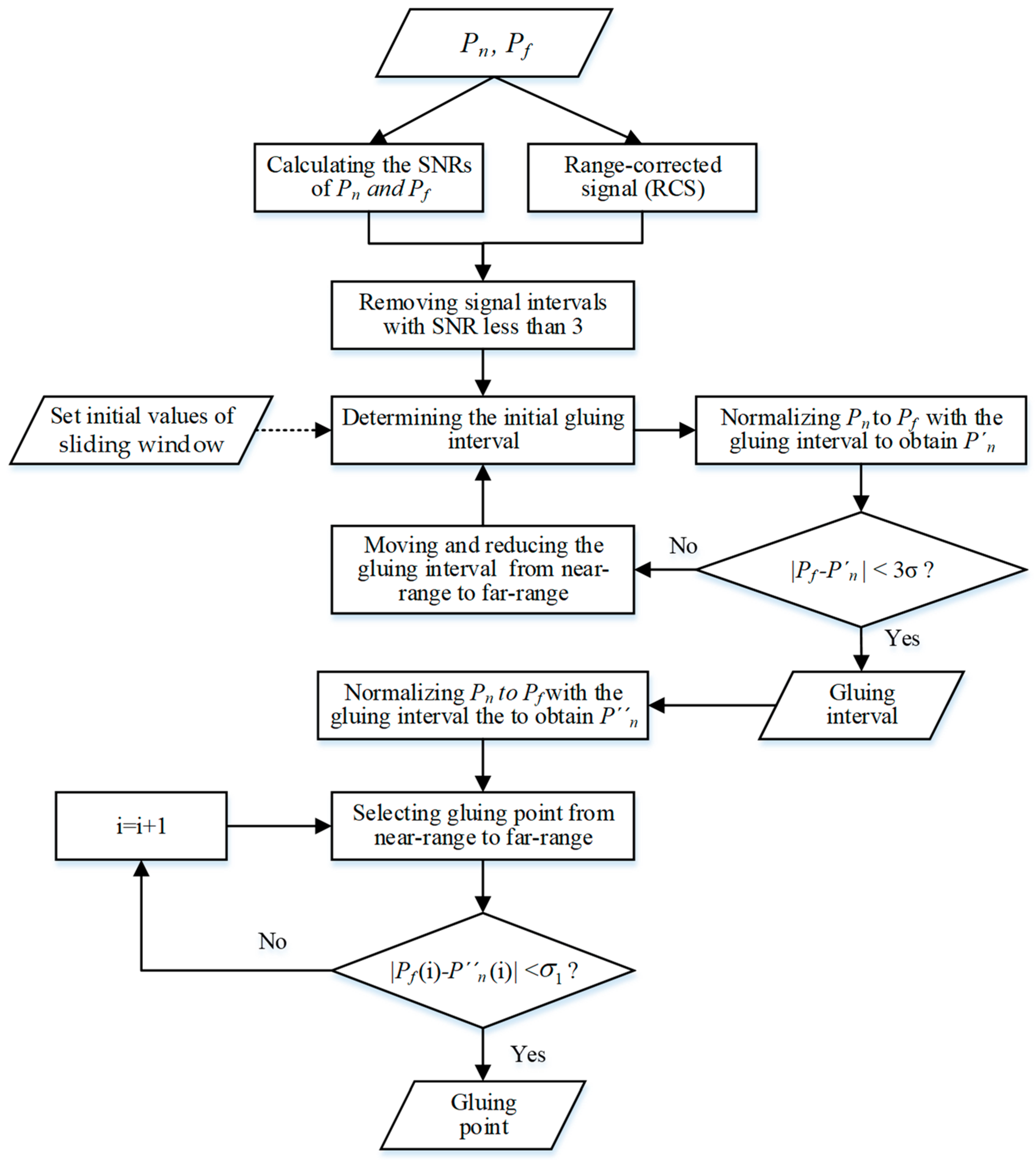
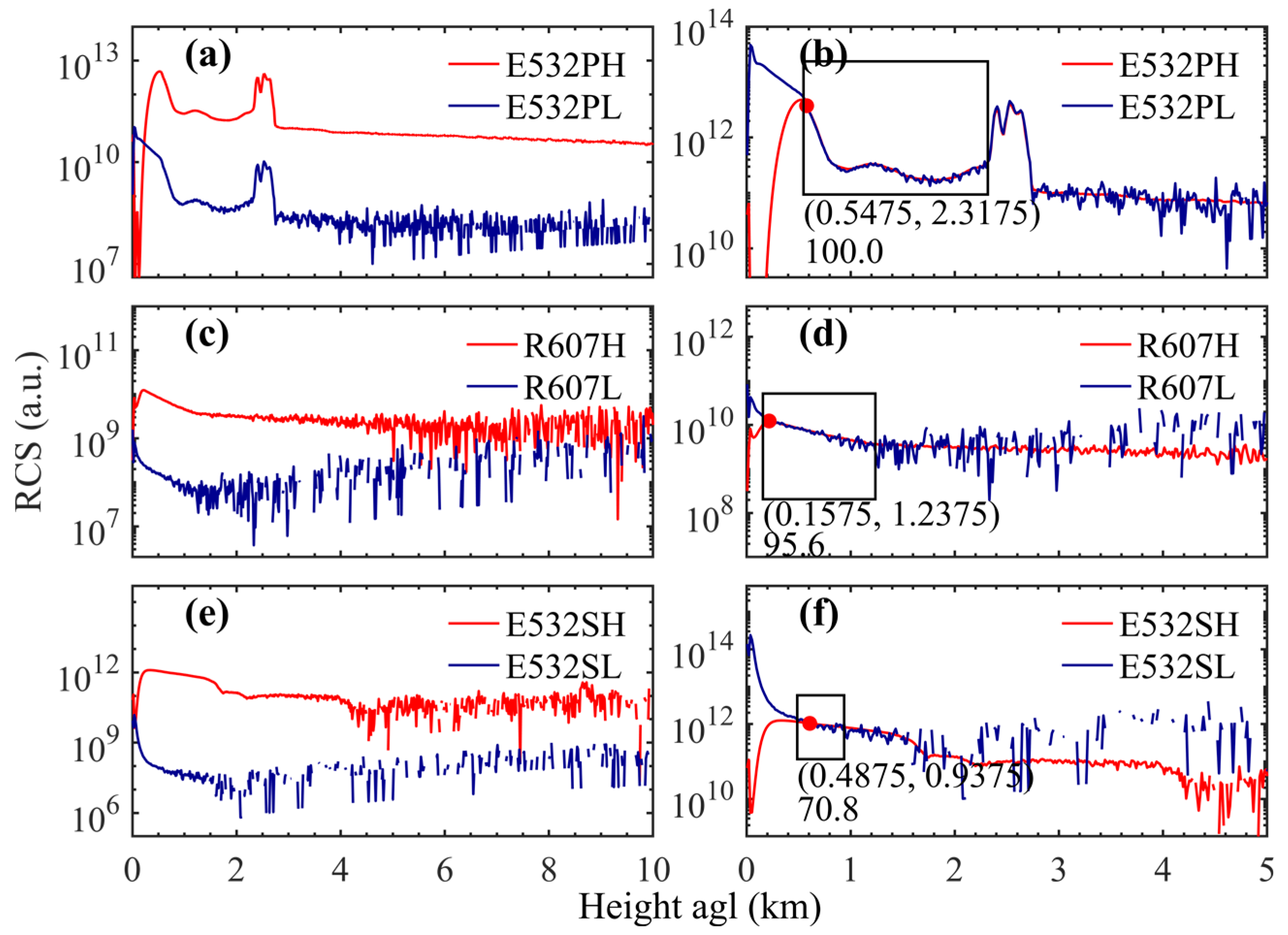
An automatic retrieval algorithm can be an effective tool for the retrieval of standardized, intercomparable aerosol optical properties from polarization Raman lidar. The introduction provided many factors that need to be considered.
Figure 1 shows the flowchart of the automatic retrieval algorithm. Signal preprocessing is required in the first stage of retrieval of the optical data products. This step mainly includes trigger delay correction, dead-time correction, overlap correction, background subtraction, and signal gluing (if needed) [25,28]. The preprocessing below is the same. Then, the SNR can be calculated, and lidar signals of poor SNR will be removed.
Clouds and aerosols can be distinguished by the differences in their optical properties. There exists a difference between separating clouds and aerosols from measured optical properties (direct observation) or separating them on the basis of retrieved physical properties (indirect observation), as it is something that can be performed after the optical data are analyzed with respect to physical properties. The profiles of meteorological data (temperature and pressure profile) are calculated with a standard atmospheric model [29]. Raman and Klett/Fernald’s methods [23,30,31] are used to retrieve aerosol optical properties according to whether the Raman signal is valid. If the Raman signal is valid, the Raman method is used to retrieve aerosol optical properties. Otherwise, the Klett/Fernald method with the assumed lidar ratio will be used.
In the processes of signal gluing and Rayleigh fit, there are many steps in which retrieval parameters need to be determined, which can significantly affect the quality of retrieved aerosol optical properties. We describe the two algorithms in detail below.

2.1. Gluing

As the signal intensity of aerosol lidar is inversely proportional to R2 (R is the range), lidar signal can cover a large dynamic range. However, at present, there are limitations of single data acquisition channels in terms of covering such a large dynamic range [25]. This situation often leads to the saturation of detectors in the near-range of a lidar or a poor SNR in the far-range of a lidar. In order to solve this issue, a second detection channel can be used to compensate for the saturation of detectors. For example, one analog channel can be combined with one photon-counting channel, or two photon-counting channels with different attenuations can be installed. In this way, one channel is used to ensure that signals at near range are detected without causing saturation of the detector. We label this signal as P n . The other channel is mainly used to ensure that signals are detected with a high SNR at the far range. We label this signal as P f . The signal gluing is then used to combine. P n and P f to obtain a vertical signal-profile of large dynamic range.
The key step of automatic gluing is to identify the best gluing interval. The gluing process finally results in one signal profile. The normalization is strongly influenced by the SNR of P n and P f [25]. Since the SNR of a lidar signal at the near range is significantly higher than that at the far range, the gluing interval is preferentially selected at the near range. In this study, a dynamic sliding window in the automatic gluing algorithm is used to search for a suitable gluing interval, and the gluing point is determined in the gluing interval. The automatic gluing algorithm can search many suitable gluing intervals and give scores to these gluing intervals. The gluing interval with the highest score is selected as the final gluing interval. The scoring rules for gluing are introduced in Section 3.2.3.
Figure 2 shows the flowchart of the automatic gluing algorithm. The gluing is based on the use of the range-corrected signals (RCS). To ensure that gluing results in vertical signal profiles of high quality, the algorithm searches in the signal interval where the SNR is greater than 3. We set a large initial sliding window and use this interval to calculate the ratio of P n to P f . We use this ratio to normalize P n to P f with the calculated ratio P n , then subtract P n from P f and calculate the standard deviation σ of | P f P n | . The algorithm counts the number of data points where | P f P n | < 3 σ . If that number accounts for more than 95% of the total number of points in the interval, the gluing interval has been found. Otherwise, the sliding window is moved to a new height interval, the length of the gluing interval is reduced, and the previous computation steps are repeated until a suitable gluing interval is found. After finding the gluing interval, the ratio is used to normalize P n to P f , and we obtain P n , and search for gluing points from near-range to far-range. The standard deviation ( σ 1 ) of | P f P n | is calculated. If | P f P n | < σ 1 , that point is the gluing point. The synthetic data is generated with the gluing interval and gluing point.
Figure 3 is an example of gluing of P n and P f . Figure 3a,c,e show the signals of the parallel polarization, Raman, and cross-polarization channels with different SNR, respectively. Figure 3b,d,f are the gluing results. The automatic gluing algorithm can find a suitable gluing interval and gluing point. The black box marks the signal gluing interval. The red point is the gluing point. The signal P n is normalized to the signal P f with the gluing interval, then the signal is glued with gluing point. The dynamic range of the glued signal is significantly improved. In addition, a comprehensive score of signal gluing is given to assess the procession of signal gluing.

2.2. Rayleigh Fit

The molecules in the atmosphere are taken as reference for calculating aerosol optical properties from Raman lidar signals. The lidar signal is normalized to the Rayleigh scattering signals by the nitrogen molecules. This calculation step is called Rayleigh fit. The reference-height interval of the Rayleigh fit needs to be selected in a height region that is free of aerosols, i.e., pure molecular atmosphere. The uncertainties caused by the Rayleigh fit propagate to the retrieved aerosol optical properties.
A high SNR of the lidar signals allows for identifying with high certainty an atmospheric region that is free of aerosols. We use a SNR larger than 3 as a benchmark. In this study, we explain the gradient-based dynamic window method (GDWM). We developed the GDWM for the automated determination of the reference height interval of the Rayleigh fit. We also evaluate the reliability of the GDWM.
The atmospheric molecular signal is calculated with the use of a standard atmospheric model [29]. In the GDWM, the ratio of the lidar signal (particles plus molecules) and the pure atmospheric molecular signal is calculated. Ideally, when there are no aerosol particles in the atmosphere, this ratio should have a constant value and the slope of this ratio should be zero. However, random signal noise results in signal uncertainty. This uncertainty will be propagated to the ratio. The slope of the ratio this will vary around 0.
Figure 4 shows the flowchart of the Rayleigh fit procedure. In the first step, the lidar signals are preprocessed and the SNR of the signal is calculated. Then, the ratio of the lidar signal to the atmospheric molecular signal is calculated. The uncertainty and the slope of the ratio are calculated next. We then determine the threshold of the slope of the ratio. If the absolute value of the slope is less than this threshold value and if the SNR of the signal is greater than 3, this interval is a candidate for the Rayleigh fit. The automatic Rayleigh fit algorithm proposed in this study can search many suitable Rayleigh fit intervals, and give scores to these Rayleigh fit intervals. The Rayleigh fit interval with highest score is selected as the final Rayleigh fit interval. The scoring rules for Rayleigh fit is introduced in Section 3.2.5.
In this study, a dynamic sliding window is used to search for particle-free areas in the lidar signal. Within the Rayleigh-fit height interval, the normalized lidar signal should vary around the atmospheric molecular signal, as the result of statistical noise in the lidar signals. In the regions that contain aerosol-particles, the signal intensity should be larger than the atmospheric molecular signal. If the above conditions are met, this sliding window defines the Rayleigh fit interval. If above two conditions are not met, the length of the window will be reduced and move from the far-range to the near-range, and the above steps will be repeated until a suitable Rayleigh fit interval has been found.
Finally, if no suitable Rayleigh fit interval can be found ever after testing all height regions that may be suitable for this procedure, the lidar-signal profile will be flagged and not used for further data processing. In most cases, more than one Rayleigh fit interval will be suitable for the next stage of data processing. In this case, we score each suitable Rayleigh fit interval and find the most suitable Rayleigh fit interval based on its comprehensive score. The scoring procedure will be explained in Section 3.2.5.
Figure 5 shows examples of Rayleigh fit. The green-shaded region shows the Rayleigh-fit interval of the signal. Figure 5a shows a signal of relatively good SNR. There is no aerosol above 5 km height, and the Rayleigh fit interval is very large. Figure 5b shows a signal with a cloud layer at approximately 3~4 km above ground. The SNR above the cloud is very poor. For this signal, the algorithm can also find a suitable Rayleigh-fit interval. Figure 5c shows a cloud layer between 6 and 8.5 km. In this case, the intervals between 9 km and 10 km, and between 2 km and 6 km are suitable for the Rayleigh fit. Considering that the computation of the aerosol profile consists of integrating from the reference point to the near-range, the reference point at the far-range may obtain more information (such as a cloud). Therefore, the height ranges from 9~10 km is chosen for the Rayleigh fit interval.
Figure 5d–f show the differences between the lidar signals and the atmospheric molecular Rayleigh fit signals for the three examples shown in Figure 5a–c. It can be seen that the lidar signal is distributed above and below the atmospheric molecular signal, which shows the feasibility of the Rayleigh fit.

3. Quality Assessment Method

Quality assurance of retrieved aerosol optical properties mainly includes factors such as lidar system performance, retrieval algorithm and meteorological condition at the observation site. These factors can be divided into two categories, those that show static characteristics and those that show dynamic characteristics. In contrast to the dynamic factors, the static factors are not influenced by the experimental environment, state of the atmosphere and weather conditions.
The static characteristics pertain to instrument characteristics. It contains trigger delay, transmitter–receiver alignment, linearity of the photo-receiving modules with respect to the optical input, whether there is Raman signal, crosstalk between elastic and Raman channel (called Raman crosstalk E-R), crosstalk between parallel polarization and cross-polarization channel (called polarization crosstalk P-S), and overlap between emitter unit and receiver unit.
The dynamic characteristics mainly include dead-time effect, background, signal gluing, Rayleigh fit, electronic interferences and meteorological data.
A scoring and weighting scheme is proposed to assess the quality of the retrieved aerosol optical properties. The score of each influencing factor ranges from 0 to 100, where 100 denotes complete reliability. The weight values are assigned to each factors according to their importance. Then, a weighted average method is used to obtain the comprehensive score of the retrieved aerosol optical properties. This comprehensive score represents the reliability of the retrieved aerosol optical properties.
In order to determine the score and the weight of each influencing factor, we simulated Raman lidar signals at 355 nm, 386 nm, 532 nm and 607 nm. Table 1 shows the main parameters of the simulated signal profiles of a Raman lidar.
Figure 6 shows a typical atmospheric scene. A planetary boundary layer (PBL) is located between 0 and 2 km height above ground level (agl). A cirrus is located between 8 and 9 km agl. In the PBL, the lidar ratio at 355 nm and 532 nm are set to 65 sr and 75 sr [32]. The linear PDR at 355 nm and 532 nm are set to 0.02 and 0.03 [33]. In the cirrus, the lidar ratio at 355 nm and 532 nm are 20 sr [34], and the linear PDRs at 355 nm and 532 nm are set to 0.3 and 0.35, respectively [35].
Figure 7 shows the RCS for this simulated scenario. Shown are the Mie-scattering parallel polarization (355 nm P, 532 nm P), cross-polarization (355 nm S, 532 nm S), and Raman signals (386 nm, 607 nm).

3.1. Assessment of Static Characteristic Factors

3.1.1. Trigger Delay

Trigger delay is caused by the latency between the laser-emitting light pulses and the start of data acquisition. This delay directly affects the atmospheric range measurements, i.e., the distance from where a signal originates and how that affects the vertical profile [25]. We simulated the effects of trigger delay deviation (from the true value) of −500 ns, −300 ns, −100 ns, 100 ns, 300 ns, and 500 ns on retrieved profiles of aerosol optical properties.
Figure 8 shows the relative error in aerosol optical properties caused by trigger delay. The misalignment in the signal range in this example has been corrected. We find that trigger delay has a significant influence on the measured aerosol extinction coefficients at near-range. This result is consistent with the conclusions of previous studies [18]. For example, a trigger delay deviation of 100 ns can cause a relative error of aerosol extinction coefficient larger than 100%. Therefore, trigger delay should be given a large weight when evaluating its influences on the retrieved aerosol extinction coefficient.
The influence of trigger delay on the aerosol backscatter coefficient is relatively small. When the trigger delay deviation is less than 300 ns, the relative error of the aerosol backscatter coefficient is less than 20%. The influence of the trigger delay on the lidar ratio and the linear PDR shows the same pattern as the aerosol extinction coefficient and backscatter coefficient, respectively. The influence of the trigger delay on the VDR is mainly the dislocation of the atmospheric range, and the dislocation is comparably small. In addition, the larger the absolute trigger delay, the larger its influence on aerosol optical properties is.
The influence of trigger delay can be corrected efficiently if the true value of the trigger delay is known. In actual measurements, the delay jitter between the laser pulse and the trigger signal is not stable; therefore, the trigger delay is not fixed. Therefore, the trigger delay needs to be monitored constantly during lidar operation. When the true trigger delay is provided, the score for trigger delay is set to 100; otherwise, it is set to 0.

3.1.2. Transmitter–Receiver Alignment

The transmitter–receiver alignment significantly affects the lidar signal at the near-range [36]. The alignment can be determined using a telecover test [37,38]. In this telecover test, the telescope is generally divided into four quadrants with the use of light shields. Misalignment of the transmitter-receiver unit [15,18,39] may lead to a distortion of the received signals; thus, retrieval results will be greatly affected. In the telecover test, signals are obtained from the four quadrants. These four quadrants are commonly referred to as north, south, east and west. The relative error of the four-quadrant signals to their mean signal can be calculated from the acquired signals. If the mean relative errors of the signals from the four quadrants are less than 20% between 0.5 km and 2 km, the score is set to 100; otherwise, the score is set to 0.

3.1.3. Linearity

The linearity of the signal response of the detector system is an important factor affecting the intensity of the measured return signal. In the ideal case, the power of the return signal (echo) and the measured photons (or voltage value at the detector output) are linearly related to each other. That is, when the strength of the echo signal of aerosol lidar increases, the strength of the detected signal also increases proportionally. However, the nonlinearity of detector response may occur for some reasons. For example, the echo signal is so strong that the detector system becomes saturated. In the most extreme case, no signals can be detected during a specific time. As another example, the optical path is not assembled properly.
To check the linearity of the detector unit, a self-test is required. Raman signals are comparably weak. For this reason, we only consider the nonlinearity of the elastic-backscatter signals in our simulations. We simulated six scenarios in which the signal strength is reduced by 1%, 2%, 5%, 10%, 15%, and 20%.
Figure 9 shows the relative errors of aerosol optical properties caused by the nonlinearity of the detector unit of the lidar system. If the signal strength is reduced by 10% (5%), the maximum relative errors of the aerosol backscatter coefficients at 355 nm and 532 nm are approximately 30% (15%) and 17% (8%). The maximum relative errors of the lidar ratios at 355 nm and 532 nm are approximately 44% (18%) and 20% (9%), respectively. The maximum relative errors of the linear PDRs at 355 nm and 532 nm are approximately 25% (10%) and 8% (3%), respectively.
When the signal strength is reduced by 2%, the maximum relative errors of the aerosol optical properties stay within 10%. When the signal strength is reduced by 20%, the maximum relative errors of the aerosol optical properties become larger than 20%., and even become larger than 100% in some cases. These results show that the linearity of the detector unit has a relatively large influence on the aerosol backscatter coefficients, lidar ratios, and linear PDRs.
The nonlinearity of the detected elastic-backscatter signals has little effect on the aerosol extinction coefficient retrieved using the Raman method and the linear VDRs. The approximate scoring scheme that is used for evaluating the linearity of signal acquisition is as follows: If the mean loss of signal strength is less than 2% between 0.5 and 2 km height agl, the score is set to 100. If the mean loss of signal strength is larger than 20%, the score is set to 0. Otherwise, the score can be calculated using a simple linear equation.

3.1.4. Raman Signal

The SNR of the Raman signal determines which retrieval method is used (see Figure 1). When the SNR of the Raman signal is ok, the Raman method [1,23] is used to retrieve aerosol optical properties. Otherwise, the Klett/Fernald algorithm [22,30,31,40] is used. In contrast to Raman lidar and the Raman method, the lidar ratio (extinction-to-backscatter ratio) needs to be assumed in the Klett/Fernald algorithm. This assumed value of the lidar ratio likely will be different from the true value. Thus, additional uncertainty will be introduced to the retrieval results obtained with the Klett/Fernald algorithm compared to the results obtained with the Raman method. Therefore, the score of aerosol optical properties retrieved from the Raman method is higher than those retrieved using the Klett method. In the calculation of the aerosol extinction coefficient with the Raman method, it is necessary to take the derivative of the Raman signal. So, the influence of the Raman signal noise on the retrieved aerosol extinction coefficient is greater than that on the aerosol backscatter coefficient. Therefore, if the Raman method is used, the score is set to 80 for the aerosol extinction coefficient and 100 for the aerosol backscatter coefficient.

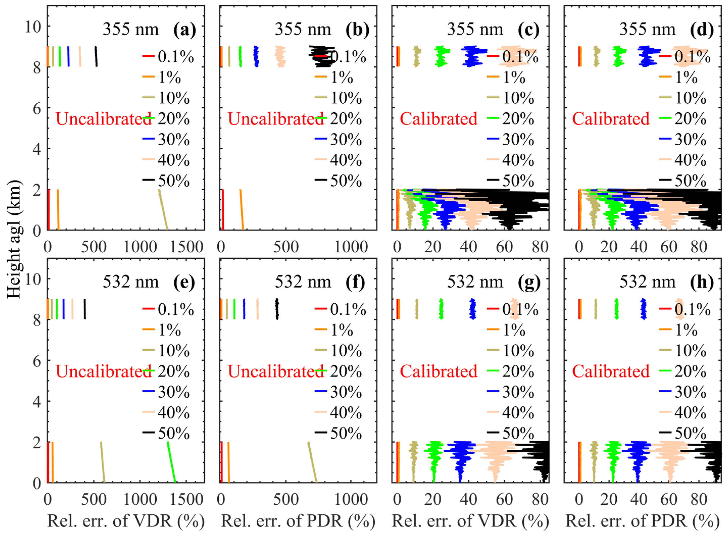
3.1.5. Polarization Crosstalk

Polarization crosstalk can be the result of, e.g., non-ideal beam splitters, the extinction ratio of polarizing beam splitters being limited, or contamination of the lens. As a result of such effects, a certain fraction of the parallel-polarized signal may be misdirected into the perpendicular-polarized detection channel [41]. The Raman retrieval algorithm [10,23] shows that such polarization crosstalk has no effect on the retrieval of aerosol extinction, backscatter coefficients, and the lidar ratio. However, this crosstalk has a significant effect on the linear VDR and linear PDR.
In this study, we discussed the effect of polarization crosstalk on retrieval results under two circumstances: one is under the circumstances when the depolarization ratio is calibrated, and the other is under the circumstances when the depolarization ratio is uncalibrated. Generally speaking, the polarization of the lidar signal needs to be calibrated before the signals are analyzed. The theoretical value of the molecular depolarization ratio is known, such as approximately 0.00376 at 532 nm [42,43]. The polarization properties of the lidar system are usually determined in clean-air conditions, i.e., we look for pure molecular atmospheric conditions for instrument calibration. The difference between the measured molecular depolarization ratio and the theoretical value of the molecular depolarization ratio is then used as the calibration value of the lidar system. In this study, we evaluated the effect of polarization crosstalk on the linear VDR and linear PDR by simulating different polarization cross talks, i.e., 0.1%, 1%, 10%, 20%, 30%, 40%, and 50%.
Figure 10 shows the relative errors of the linear VDR and linear PDR caused by polarization crosstalk. We consider, in one case, depolarization ratio calibration. In another case, we do not consider depolarization ratio calibration. Figure 10a,b,e,f shows the relative error of the linear aerosol depolarization ratio for the case when the depolarization ratio is not calibrated. The results show a comparably large effect of polarization crosstalk. Polarization crosstalk as low as 1% can lead to more than 100% relative error of the linear VDR and linear PDR. Therefore, the depolarization ratio needs to be calibrated before data retrieval. Figure 10c,d,g,h show the result when the depolarization ratio is calibrated. We see a significantly lower impact of the polarization crosstalk on the linear VDR and linear PDR. If the polarization crosstalk is less than 10%, the relative errors of the linear VDR and linear PDR stay within (approximately) 10%, and we set the score to 100. When the polarization crosstalk is larger than 40%, the relative errors of the linear VDR and linear PDR are larger than (approximately) 40%. We set the score to 0. For any other value, we calculate the score using a simple linear equation.

3.1.6. Raman Crosstalk
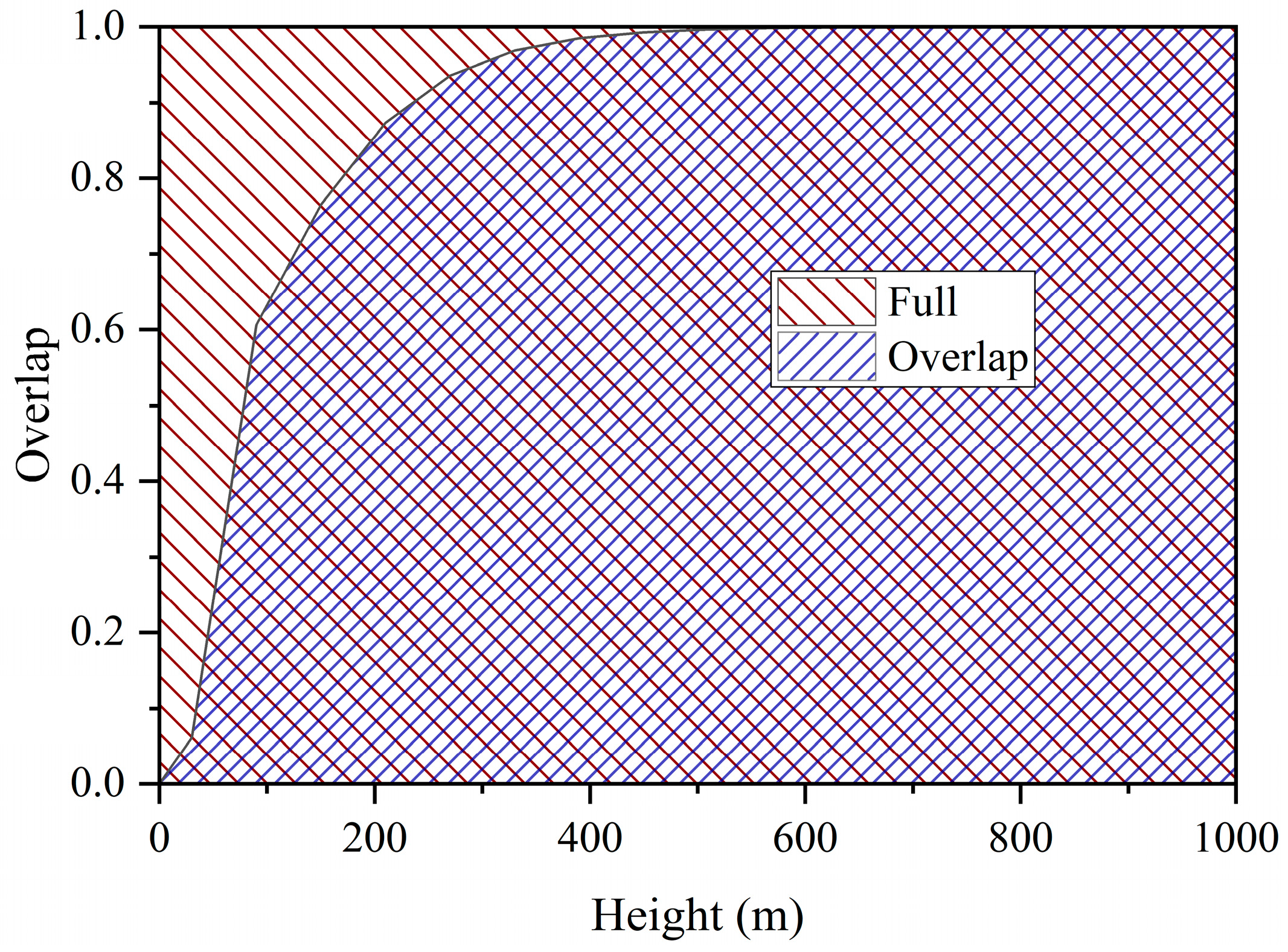
Raman-signal crosstalk results from the elastic-backscatter signals misdirected into the Raman channels for some reason, such as limited light-suppression level of the interference filter, leading to leakage of light in the optical path.
Figure 11 shows the influence of 4 different Raman crosstalk levels (10−8, 10−7, 10−6, 10−5) on the retrieved aerosol optical properties. The result shows that Raman crosstalk significantly influences the aerosol extinction coefficients and lidar ratios but has little influence on the linear particle depolarization ratio.
When Raman crosstalk is 10−5, the maximum relative error of the aerosol extinction coefficients and lidar ratios between 8 and 9 km at 532 nm are larger than 100%. The maximum relative errors of the aerosol extinction and backscatter coefficients, lidar ratios, and linear PDR at 355 nm are less than (approximately) 20%. In this case, we set the score to 20.
When Raman crosstalk is 10−6, the maximum relative errors of the aerosol extinction and backscatter coefficients, lidar ratios and linear PDR at 355 nm are less than 5%. The maximum relative errors of the aerosol extinction coefficients between 8 and 9 km at 532 nm are larger than 10%. In this case, we set the score to 60.
When the Raman crosstalk is less than 10−7, both the maximum relative errors of the aerosol extinction, backscatter coefficients, lidar ratios, and linear PDRs at 355 nm and 532 nm are less than 2%. In this case, we set the score to 100.
If the Raman crosstalk is different from these values, we use the logarithmic-linear equation to calculate the score, see Equation (1).
S = 40 log ( x ) 180
where S represents the score for Raman crosstalk, and x represents Raman crosstalk.

3.1.7. Overlap

The overlap between the laser beam and the field-of-view of the receiver unit is incomplete in the near field of the lidar [44,45,46]. As a consequence, signal intensity will be reduced in the overlap region. The shorter the distance at which full overlap is achieved, the more information the lidar signal can provide.
This intensity loss with height can be described by the overlap function. We propose an area-integrated ratio method to calculate the score that describes the quality of the overlap.
Figure 12 shows an example of the diagram of the area-integrated ratio method. The blue-hashed part describes the area between the overlap function in dependence on distance from the lidar and horizontal coordinate. The red slash marked part is the area between the overlap function with a value equaling one and a horizontal coordinate. At present, the majority of lidar’s full overlap distance is less than 1000 m. Therefore, we set the integration interval of the horizontal coordinate (which describes the distance) to 0–1000 m. We calculate the two areas, divide the numbers, and multiply the result by 100. This final number describes the overlap score.

3.2. Assessment of Dynamic Characteristic Factors

3.2.1. Dead-Time Correction

The dead-time effect of photons is determined by the operation mode of the detector; generally, photomultipliers are used for lidar applications. When a photon impacts the photo-cathode of a photomultiplier, an electrical pulse is generated [25]. If a large number of photons arrives at the photomultiplier within a given time increment and if the detector cannot discriminate each photon, then the number of detected photons is smaller than the actual number of photons that arrive at the detector head. This dead-time (τ) of the detector decides on the resolution capability of the detector. In data analysis, a dead-time correction is therefore required.
Two mathematical formulas can be used for dead-time correction, i.e., the paralyzable model and the non-paralyzable model [25]. The formulas are shown as follows.
M = N exp ( N τ )
M = N N τ + 1
where Equation (2) is used for the paralyzable model, and Equation (3) is used for the non-paralyzable model. M is the measured count rate of photons, N is the true count rate, τ is the dead-time of the detector.
As the pile-up effect is a nonlinear and quite complex process, it cannot be fully corrected using a mathematical formula if the photon count rate passes a certain threshold. If the dead-time correction is not carried out, or if the detector is saturated by a signal that is too strong, or if the photon count rate is larger than 1/τ [25], the score will be set to 0. When the photon count rate is less than 1/5τ, the pile-up effect can be corrected comparably well by mathematical formulas, and the score will be set to 100.
The pile-up effect gradually cannot be completely corrected by mathematical formulas for increasing the photon count rate. The greater the photon count rate, the less accurate the effect of mathematical correction on the quality of signal detection will be. When the photon count rate is larger than 1/5τ and less than 1/τ, the score can be calculated with a simple quadratic equation, see Equation (4).
S = 156.25 τ 2 x 1 5 τ 2 + 100
where S represents the score for dead-time, and x represents the measured count rate.

3.2.2. Background Noise

The signal noise of aerosol Raman lidar is mainly caused by sky background radiation. The sky background is mainly caused by solar radiation. Background noise can affect the SNR of the detected lidar signals and thereby add additional random errors to the retrieved data products. In this study, we use the maximum detection range where the SNR is greater than 3 to assess background noise. The larger the maximum detection range is, the higher the score (related to background noise) will be. The aerosol Raman lidar is usually used to research atmospheric characteristics below 30 km. Therefore, when the maximum detection range is larger than 30 km, the score can be set to 100. Cirrus clouds generally range from 8 to 15 km [47,48]. Therefore, if the maximum detection range reaches 15 km, the score can be set to 90. If the maximum detection range reaches 10 km, the score will be set to 80. If the maximum detection range reaches 5 km, the score will be set to 60. Otherwise, the score of background noise can be obtained using a simple linear interpolation.

3.2.3. Gluing

The key step of signal gluing is to find the optimum gluing interval and gluing point, see Section 2.1. Two parameters are used to assess the reliability of signal gluing: the length of the gluing interval and the mean SNR within the gluing interval. The longer the length of the gluing interval, the higher the reliability of signal gluing. Signals with high SNR will reduce the uncertainty of signal gluing. As the SNR of the lidar signals at the near-range is generally higher, selecting the gluing interval closer to the near-range of the lidar is preferred. When the interval length is larger than the length threshold (the threshold is set to 1500 m in this study), the score of signal gluing is set to 100. Otherwise, the score of the gluing intervals is assessed using a cubic function, see Equation (5).
S = 100 1 1500 x / 1500 3
where S represents the score for gluing intervals, and x represents the gluing intervals.
When the mean SNR is larger than the SNR threshold (the threshold is set to 20 in this study), its score is set to 100. When the mean SNR is less than 2, the score is set to 0. In all other cases, the score of the mean SNR can be obtained using a linear function. The gluing score is the weighted average of these two scores.

3.2.4. Meteorological Data
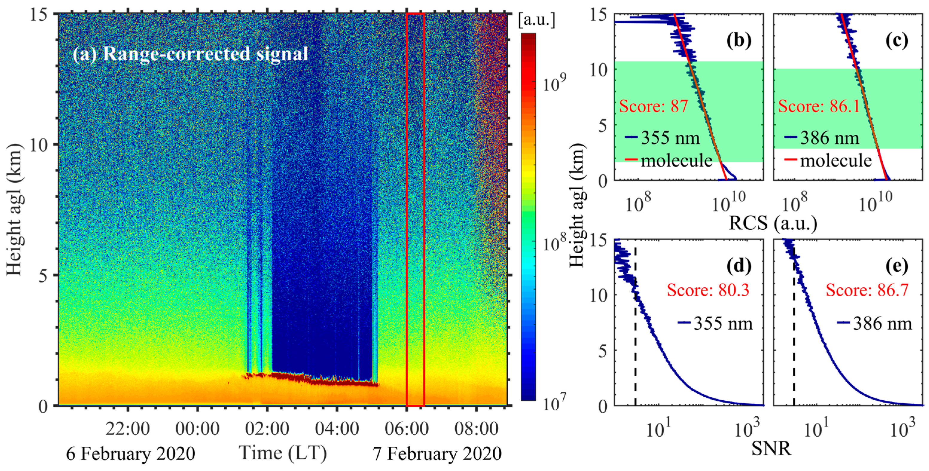
Meteorological data are usually used to calculate atmospheric density, which is used to calculate molecular backscatter coefficients and extinction coefficients. These parameters are taken as reference in the retrieval of the optical data products. Thus, if the reference values are inaccurate, the quality of the final data products will be affected, too.
The two methods commonly used for obtaining meteorological data are radiosonde measurements [49] and standard atmospheric models [29]. Radiosondes provide true meteorological data in the sense that several instruments (combined in a radiosonde) are used for measurements of atmospheric state parameters. Meteorological data obtained by a standard atmospheric model are close to the true values. If a standard atmospheric model is used, temperature and pressure at the observation site are required as input. The deviation of the input temperature and pressure from the true values directly affects the accuracy of the final data products. In our study, we applied different levels of deviation of temperature and pressure from the true value and simulated how these deviations affect the quality of the retrieval results.
Figure 13 shows the relative errors of aerosol optical properties caused by temperature deviations of −15 °C, −10 °C, −5 °C, 5 °C, 10 °C, and 15 °C. The results presented in Figure 13 show that the temperature deviation has little effect on the linear VDR and has a slight influence on the aerosol extinction and backscatter coefficients, the lidar ratio, and the linear PDR. Relative errors of all these parameters are less than 20%.
Figure 14 shows the relative errors of the aerosol optical properties caused by pressure deviations. We simulated deviations of −150 hPa, −100 hPa, −50 hPa, 50 hPa, 100 hPa, and 150 hPa, respectively. The influence of the pressure deviations on the aerosol optical properties is similar to that of temperature deviations.
In conclusion, the score is set to 100 if radiosonde data are used. The temperature and pressure profiles calculated using a standard atmospheric model have some differences from the true values; therefore, the score is less than that of the radiosonde. If temperature and pressure data at the observation site (at ground level near the lidar) are used, the score is set to 70. If there are no measurements of meteorological state parameters at the observation site, the temperature and pressure at the observation site need to be assumed, and the score is set to 40. When calculating the linear VDR, the weight of meteorological data items is assigned to 0. When calculating all other aerosol optical properties, meteorological data can be assigned a relatively small weight.

3.2.5. Rayleigh Fit

The Rayleigh-fit interval is generally selected in the aerosol-free area; for details, see Section 2.2. Two parameters are used to assess the quality of the Rayleigh fit: the fit interval and the location of the reference point. A longer fit interval can reduce the uncertainty of the retrieval results. When the length of the Rayleigh fit interval is 0 km, 2 km, and (larger than) 5 km, the score is set to 0, 60, and 100, respectively. When the length of the Rayleigh fit interval is different from these three values, the score is obtained by a simple linear interpolation method. Since the data retrieval of aerosol lidar is integrated from the reference point to the near-range, the higher the position of the reference point, the more spatial information contained in the retrieval result. When the position of the reference point is at 5 km, 10 km, 15 km, and (larger than) 20 km, the scores are set to 60, 80, 90, and 100, respectively. When the position of the reference point is at heights different from the ones described here, the score is obtained using a simple linear interpolation method.

3.2.6. Electronic Interference

Electronic interference affects the quality of lidar signals, which are generally produced in signals collected in the analog-mode channels. In lidar observation, it is necessary to measure the electrical noise. When the electrical interference is less than the random error of the signals, it can be ignored, and the score is set to 100. When the electrical interference is larger than the random error of the signals, if it is measured correctly and removed, the score is set to 100. In all other cases, the score is set to 0.
According to the simulations and our analysis described above, we assign a weighting factor to each influencing factor. At present, the exact weighting factor cannot be determined. However, the assigned weights reflect the importance of the various factors that influence data quality.
Table 2 finally summarizes the weighting of the different factors that influence the aerosol optical properties retrieved from Raman lidar. If the influencing factors have no effect on the aerosol optical properties, the weight is assigned to 0. If the impact of the influencing factors on the aerosol optical properties is obviously relatively small (large), then a small (big) weight is assigned. In other cases, an average weight value is assigned.

4. Results

4.1. Aerosol Raman Lidars

In this study, two different Raman lidars are selected to evaluate the proposed quality assessment algorithm for different observation scenarios.
Table 3 shows the main information of observation sites, which are at a high mountain site and in a suburb of Beijing. The operating wavelengths of the two Raman lidars are 355 nm and 532 nm. The Raman channels are at 386 nm and 607 nm.
The two Raman lidars were calibrated before the field measurements began. Therefore, the lidar system was good, and the polarization crosstalk and Raman crosstalk were small enough to be ignored. The trigger delay was measured. The position of the optical axis defined by the transmitter–receiver unit was aligned. The score of each influencing factor mentioned above is set to 100. The meteorological data were calculated using standard atmospheric models. Temperature and pressure at the observation stations were estimated, and the score of the meteorological data was set to 40.

4.2. Experimental Assessment

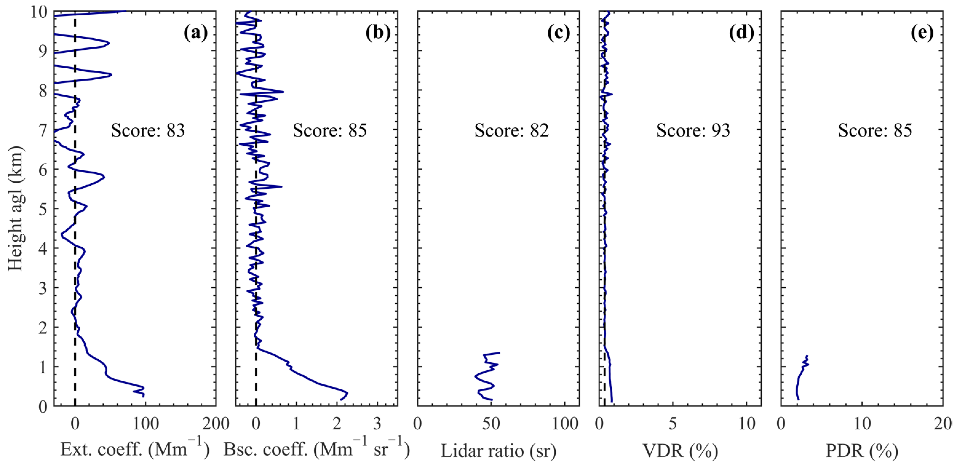
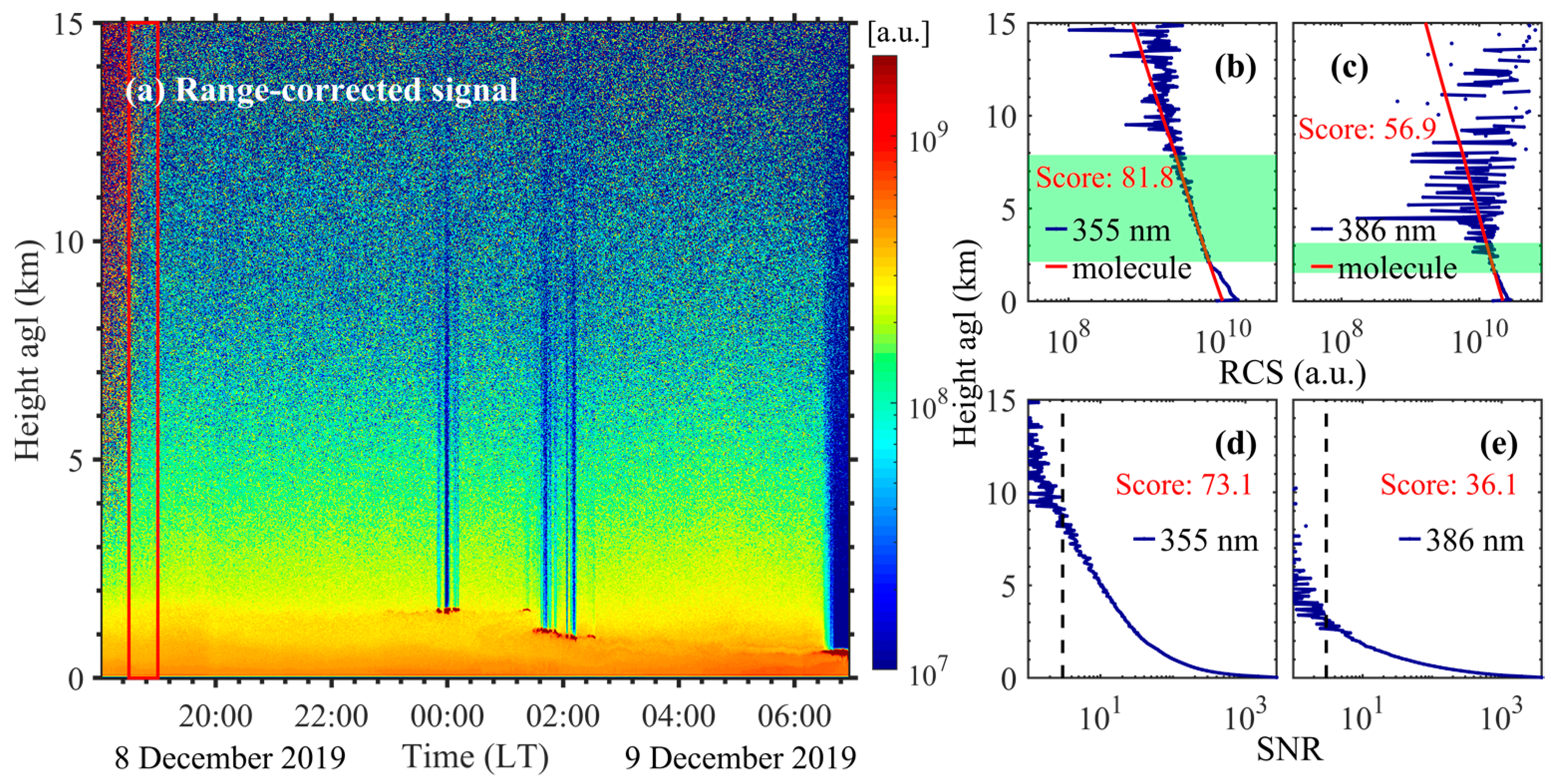
4.2.1. High-Mountain Environment

The Raman polarization lidar that operates at 355 nm was located at Lijiang (26°43′N, 100°01′E). The field site is at approximately 3170 m agl. The aerosol concentration in the air was comparably low during the time of the observations in this study. Accordingly, light-scattering was mainly due to molecules [13]. The lidar contains three detection channels: 355 nm parallel polarization channel (E355P), 355 nm cross-polarization channel (E355S), and nitrogen Raman channel (R386) corresponding to the laser emission wavelength of 355 nm. This lidar has been calibrated and compared with the lidar at the EARLINET lidar station of Naples [13,50].
Figure 15 shows the results of the lidar observation on 6 and 7 February 2020. Figure 15a shows the range corrected signal (RCS) at 355 nm between 20:00 and 08:50 (local time, LT). Aerosols were mainly located below 2 km agl. A cloud layer was detected at approximately 1 km agl between 01:20 and 05:10 LT on 7 February 2020, which may have formed as the temperature dropped and humidity increased at night. We selected the signals collected between 06:00 and 06:30 LT on 7 February 2020 for our analysis; see the red box in Figure 15a.
Figure 15b,c show the profiles of the RCS at 355 nm and 386 nm, respectively. The results show that the Rayleigh fit of the RCS both at 355 nm and 386 nm shows well. The Rayleigh fit intervals of the signals at 355 nm and 386 nm are between 1.65 and 10.71 km agl, and between 2.85 and 10.05 km agl, respectively. The corresponding scores are 87 and 86.1.
Figure 15d,e show the signal-to-noise ratio (SNR) corresponding to Figure 15b,c, respectively. The results show that the maximum detection range at 355 nm and 386 nm, where the SNR is greater than 3, is approximately 10 km and 13 km, respectively. The scores of the background noise for the lidar signals at 355 nm and 386 nm are 80.3 and 86.7, respectively.
Figure 16 shows the aerosol optical properties measured between 06:00 and 06:30 LT on 7 February 2020. The background noise in the sky accordingly was low, and the SNR was relatively high (see Figure 15). In addition, the Rayleigh fit of signals shows well there was no electrical interference in the signals.
Though the score of the meteorological data is low, the deviation of temperature and pressure (from their presumably true values) has little influence on the measured aerosol optical properties (see Figure 13 and Figure 14), and the weight of meteorological data is small.
In summary, the score of each aerosol optical property is relatively high. The linear VDR has the highest score because this parameter is only related to the reliability of the parallel polarization and cross polarization signals.
Figure 17 shows the results of the lidar observation on 8 and 9 December 2019. Figure 17a shows the RCS between 18:00 and 06:55 LT. Aerosols were mainly distributed between approximately 0 and 2 km. Figure 17b,c shows the profiles of the RCS at 355 nm and 386 nm between 18:30 and 19:00 LT on 8 December 2019. This time is marked by a red box in Figure 17a. The Rayleigh fit intervals of the signals at 355 nm and 386 nm are between 2.13 and 7.89 km agl and 1.53 and 3.15 km agl, respectively. The corresponding scores are 81.8 and 56.9. Figure 17d,e show the profiles of SNR corresponding to Figure 17b,c, respectively. The maximum detection ranges at 355 nm and 386 nm, where the SNR is larger than 3, are approximately 8.5 km and 3 km agl, respectively. The scores of the background of the lidar signal at 355 nm and 386 nm are 73.1 and 36.1, respectively.
Figure 18 shows the aerosol optical properties between 18:30 and 19:00 LT on 8 December 2019. Sky background radiation was still relatively strong during this time as the sun had just set. Therefore, the SNR of the lidar signal was comparably low, especially for the signal at 386 nm (see Figure 17d,e). The score of the background signal is relatively low. In addition, the Rayleigh fit interval of the Raman signal is relatively short, and the score is low, too. As in the previous measurement example, the temperature and pressure at the observation station were estimated. The score of the input meteorological data is low. Therefore, the scores of the aerosol extinction coefficients, aerosol backscatter coefficients, lidar ratios, and linear PDR are relatively low compared to the scores in Figure 16.
The results presented in Figure 16 and Figure 18 show that the reliability of retrieved aerosol optical properties for every measurement is different under different observation scenarios, even with the same lidar. Therefore, it is necessary to assess the reliability of retrieved aerosol optical properties from each measurement.

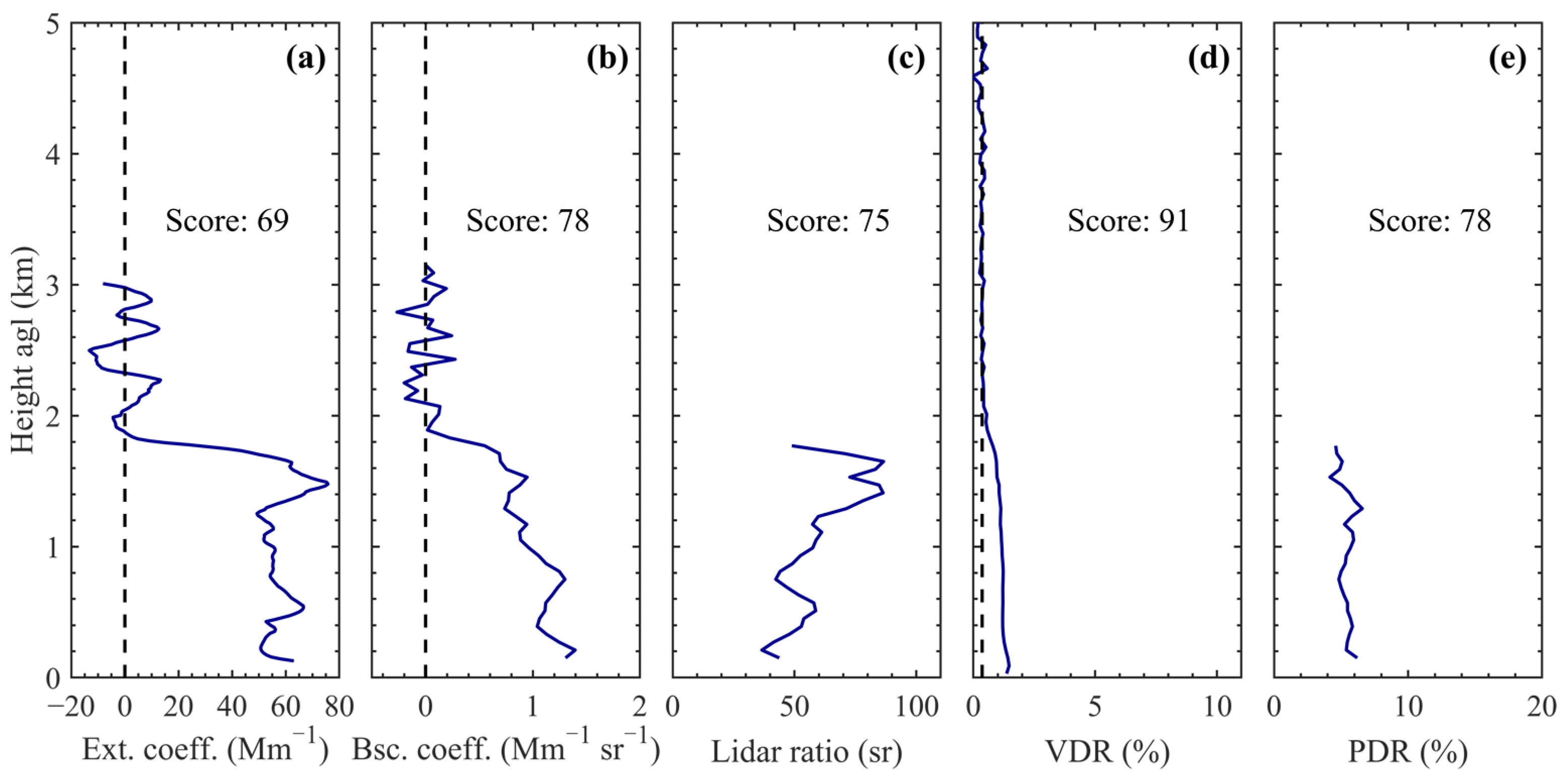
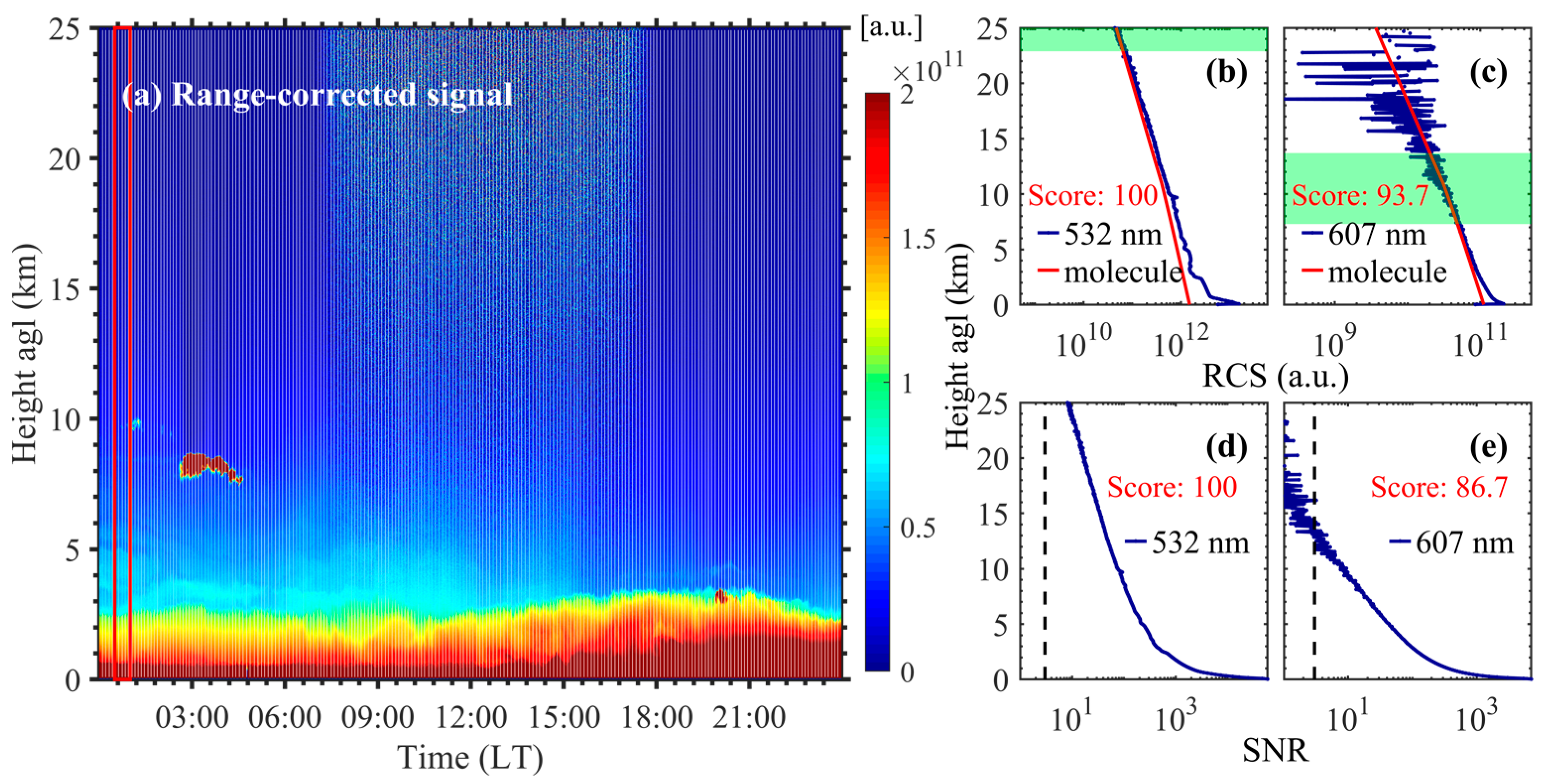
4.2.2. Suburban Environment

A second polarization Raman lidar was located at the Beijing Southern Suburb Observatory (39°48′N, 116°28′E) [51]. That system operates at 532 nm laser emission. The system contains six detection channels: 532 nm parallel-polarization channel for the near-range (E532PL), 532 nm parallel-polarization channel for the far-range (E532PH), 532 nm cross-polarization channel for the near-range (E532SL), 532 nm cross-polarization channel for the far-range (E532SH), 607 nm nitrogen Raman channel for the near-range (R607L), and 607 nm nitrogen Raman channel for the far-range (R607H).
Figure 19 shows the results of the lidar observation on 5 February 2021. Figure 19a shows the RCS. There are aerosol layers in the atmosphere up 10 km agl. The aerosol signal in Figure 19b stays above the molecular signal up to 10 km agl and shows a comparably strong polluted lower troposphere (up to 3 km agl).
Figure 19b,c show the profiles of the RCS at 532 nm and 607 nm between 00:30 and 01:00 LT, and that timeframe is marked by a red box in Figure 19a. The Rayleigh fit intervals for the signals at 532 nm and 607 nm are between 22.89 and 31.23 km agl, and between 7.29 and 13.71 km agl, respectively. The score of the Rayleigh fit for the signals at 532 nm and 607 nm are 100 and 93.7, respectively.
Figure 19d,e show the SNRs corresponding to the profiles shown in Figure 19b,c. The maximum detection distances at 532 nm and 607 nm where the SNR is larger than 3 are above 25 km for the signal at 532 nm and approximately 13 km for the signal at 607 nm, respectively. The corresponding scores are 100 and 86.7.
Figure 20 shows the aerosol optical properties between 00:30 and 01:00 LT on 5 February 2021. The Rayleigh fit of the signal shows well, and the SNR was relatively high. There was no electrical interference in the signal. The score of the optical properties is accordingly high.
Figure 21 shows the results of the lidar observation on 16 March 2021. Figure 21a shows the RCS between 00:00 and 21:40 LT. Aerosols were detected to be at least 10 km height agl. The distribution of the aerosol in the atmosphere is high, and the aerosol stratification is obvious. Clouds were detected between 7 and 12 km at approximately 10:00 to 18:00 LT.
Figure 21b,c shows the profiles of the RCS at 532 nm and 607 nm between 19:30 and 20:00 LT. This time is marked by a red box in Figure 21a. The Rayleigh fit intervals of the signals at 532 nm and 607 nm are placed between 14.67 and 21.69 km agl, and between 4.47 and 5.19 km agl, respectively. The score of the Rayleigh fit for the signals at 532 nm and 607 nm are 100 and 43.9, respectively.
Figure 21d,e are the SNRs corresponding to the profiles in Figure 21b,c. It shows that the maximum detection ranges at 532 nm and 607 nm are larger than 20 km agl and approximately 5 km agl, respectively. The corresponding scores are 94.6 and 56.8.
Figure 22 shows the aerosol optical properties between 19:30 and 20:00 LT on 16 March 2021. Two distinct aerosol layers were present in the atmosphere during that time. The intensity of the Raman signal dropped to lower values after passing through the aerosol layer. Therefore, the SNR of the Raman signal is low (see Figure 21e). The reference interval of the Rayleigh fit is short (see Figure 21c). The scores of aerosol extinction coefficient, aerosol backscatter coefficient, lidar ratio, and linear PDR are relatively low.
The results presented in Figure 20 and Figure 22 show that the scores of the retrieved aerosol optical properties for every measurement are different under different weather conditions. The proposed quality reliability assessment algorithm can distinguish the reliability of retrieval results for each measurement well.

5. Conclusions

Raman lidar allows for measuring vertically resolved profiles of important aerosol optical properties. However, the quality reliability of the retrieved aerosol optical properties is difficult to assess because of the differences in the hardware design of lidar systems, the retrieval algorithms, and the meteorological conditions at the observation site. In this study, we proposed an assessment method to evaluate the quality of aerosol optical properties measured using Raman lidar. We analyzed the factors that affect the aerosol optical properties. For each influencing factor, we give scores and assign weights. The comprehensive score of each aerosol optical properties can be obtained using the weighted average method.
A simulation study was used to analyze the factors that influence the aerosol optical properties retrieved from Raman lidar. These factors are summarized in the following.
Trigger delay has a significant influence on the measured aerosol extinction coefficient and the lidar ratio retrieved using the Raman method. Even a small deviation can result in a relative error of more than 100%. In contrast, a trigger delay has a relatively small effect on the measured aerosol backscatter coefficients and linear PDRs.
In this study, we simulated the nonlinear response of lidar for an elastic-backscatter signal. The simulation results show that it has a relatively big influence on the quality of the measured aerosol backscatter coefficients, lidar ratios, and linear PDRs.
Polarization crosstalk has no effect on the measured aerosol extinction coefficients, backscatter coefficients, and lidar ratios. When the depolarization ratio is not calibrated, it has a great influence on VDR and PDR. A 1% polarization crosstalk may result in a relative error of more than 100%, depending on the type of particle. When the depolarization ratio is calibrated, the effect of polarization crosstalk is obviously weakened. When the polarization crosstalk is less than 10%, the relative errors of the linear VDRs and PDRs at 355 nm and 532 nm remain within (approximately) 10%.
Raman crosstalk has a significant influence on the measured aerosol extinction coefficients and lidar ratios. When the Raman crosstalk is less than 10−7, both the relative uncertainties of aerosol optical properties at 355 nm and 532 nm are less than 5%. Raman crosstalk has a relatively small effect on the measured aerosol backscatter coefficients and linear PDRs.
When the meteorological data is obtained using the standard atmospheric model, the deviation of temperature and pressure of the observation station have a relatively small effect on the aerosol optical properties.
We give the score and assign weight to each influencing factor according to the simulation result and analysis.
Two Raman polarization lidars, one at a high-mountain site and one at a suburban site, were used to test the proposed quality assessment algorithm under different atmospheric pollution conditions. One instrument operates at 355 nm, and the other one operates at a 532 nm laser wavelength. The results show differences in the quality of the aerosol optical properties measured using the two lidars. Even for the same lidar, the reliability of the measured aerosol optical properties can be significantly different under different observation scenarios. Additionally, the quality assessment algorithm proposed in this study can distinguish the reliability of the retrieval results.
In the quality assurance method, simplified linear equations are used to obtain the scores of several influencing factors. Even though the simulation calculation and analysis are carried out to determine the weights of the influencing factors, there is still room for further refinement of the weights. In future work, more scenarios will be used to test the quality assurance method to obtain a more refined scoring and weight allocation scheme.

Author Contributions

Conceptualization, S.M. and X.W.; methodology, S.M. and X.W.; software, S.M.; validation, S.M. and X.W.; formal analysis, S.M., X.W., Z.Y. and L.W.; investigation, S.M. and Y.W.; data curation, S.M., Z.B., Y.C. and Y.D.; writing—original draft preparation, S.M.; writing—review and editing, X.W., D.M., Z.Y., L.W., Y.W., Z.B., Y.C. and Y.D.; funding acquisition, X.W., Z.Y., L.W. and Y.C. All authors have read and agreed to the published version of the manuscript.

Funding

This research was funded by the National Natural Science Foundation of China (NSFC) (42205130, 62275202, 62105248), the National Key Research and Development Program of China (2021YFC3090200, 2023YFC3007800), and the Innovation and Development Project of China Meteorological Administration (CXFZ2022J060).

Data Availability Statement

The datasets generated and/or analyzed during the current study are available from the corresponding author upon reasonable request.

Conflicts of Interest

The authors declare no conflicts of interest.

References

  1. Ansmann, A.; Riebesell, M.; Weitkamp, C. Measurement of atmospheric aerosol extinction profiles with a Raman lidar. Opt. Lett. 1990, 15, 746–748. [Google Scholar] [CrossRef] [PubMed]
  2. Müller, D.; Franke, K.; Wagner, F.; Althausen, D.; Ansmann, A.; Heintzenberg, J.; Verver, G. Vertical profiling of optical and physical particle properties over the tropical Indian Ocean with six-wavelength lidar: 2. Case studies. J. Geophys. Res. Atmos. 2001, 106, 28577–28595. [Google Scholar] [CrossRef]
  3. Heese, B.; Baars, H.; Bohlmann, S.; Althausen, D.; Deng, R. Continuous vertical aerosol profiling with a multi-wavelength Raman polarization lidar over the Pearl River Delta, China. Atmos. Chem. Phys. 2017, 17, 6679–6691. [Google Scholar] [CrossRef]
  4. Hu, Q.; Wang, H.; Goloub, P.; Li, Z.; Veselovskii, I.; Podvin, T.; Li, K.; Korenskiy, M. The characterization of Taklamakan dust properties using a multiwavelength Raman polarization lidar in Kashi, China. Atmos. Chem. Phys. 2020, 20, 13817–13834. [Google Scholar] [CrossRef]
  5. Fiorani, L. Lidar: A powerful tool for atmospheric measurements. J. Optoelectron. Adv. Mater. 1999, 1, 3–11. [Google Scholar]
  6. Mamouri, R.-E.; Ansmann, A. Potential of polarization/Raman lidar to separate fine dust, coarse dust, maritime, and anthropogenic aerosol profiles. Atmos. Meas. Tech. 2017, 10, 3403–3427. [Google Scholar] [CrossRef]
  7. Ansmann, A.; Baars, H.; Tesche, M.; Müller, D.; Althausen, D.; Engelmann, R.; Pauliquevis, T.; Artaxo, P. Dust and smoke transport from Africa to South America: Lidar profiling over Cape Verde and the Amazon rainforest. Geophys. Res. Lett. 2009, 36, L11802. [Google Scholar] [CrossRef]
  8. Su, T.; Li, Z.; Kahn, R. Relationships between the planetary boundary layer height and surface pollutants derived from lidar observations over China: Regional pattern and influencing factors. Atmos. Chem. Phys. 2018, 18, 15921–15935. [Google Scholar] [CrossRef]
  9. McFarquhar, G.M.; Bretherton, C.S.; Marchand, R.; Protat, A.; DeMott, P.J.; Alexander, S.P.; Roberts, G.C.; Twohy, C.H.; Toohey, D.; Siems, S.; et al. Observations of Clouds, Aerosols, Precipitation, and Surface Radiation over the Southern Ocean: An Overview of CAPRICORN, MARCUS, MICRE, and SOCRATES. Bull. Am. Meteorol. Soc. 2021, 102, E894–E928. [Google Scholar] [CrossRef]
  10. Ansmann, A.; Riebesell, M.; Wandinger, U.; Weitkamp, C.; Voss, E.; Lahmann, W.; Michaelis, W. Combined Raman elastic-backscatter lidar for vertical profiling of moisture, aerosol extinction, backscatter, and lidar ratio. Appl. Phys. B 1992, 55, 18–28. [Google Scholar] [CrossRef]
  11. Cao, Y.; Xie, C.; Wang, B.; Cheng, L.; Fang, Z.; Li, L.; Zhuang, P.; Yang, H.; Shao, J.; Jiang, H.; et al. Design and optimization of Mie scattering lidar detection system. In Proceedings of the Sixth Symposium on Novel Optoelectronic Detection Technology and Applications, Beijing, China, 3–5 December 2019. [Google Scholar]
  12. Whiteman, D.; Melfi, S.; Ferrare, R. Raman lidar system for the measurement of water vapor and aerosols in the Earth’s atmosphere. Appl. Opt. 1992, 31, 3068–3082. [Google Scholar] [CrossRef] [PubMed]
  13. Liu, F.; Yi, F. Lidar-measured atmospheric N2 vibrational-rotational Raman spectra and consequent temperature retrieval. Opt. Express 2014, 22, 27833–27844. [Google Scholar] [CrossRef] [PubMed]
  14. Xu, W.; Yang, H.; Sun, D.; Qi, X.; Xian, J. Lidar system with a fast scanning speed for sea fog detection. Opt. Express 2022, 30, 27462–27471. [Google Scholar] [CrossRef] [PubMed]
  15. Kral, L. Automatic beam alignment system for a pulsed infrared laser. Rev. Sci. Instrum. 2009, 80, 013102. [Google Scholar] [CrossRef] [PubMed]
  16. Wandinger, U.; Freudenthaler, V.; Baars, H.; Amodeo, A.; Engelmann, R.; Mattis, I.; Groß, S.; Pappalardo, G.; Giunta, A.; D’Amico, G.; et al. EARLINET instrument intercomparison campaigns: Overview on strategy and results. Atmos. Meas. Tech. 2016, 9, 1001–1023. [Google Scholar] [CrossRef]
  17. Wang, L.; Yin, Z.; Bu, Z.; Wang, A.; Mao, S.; Yi, Y.; Müller, D.; Chen, Y.; Wang, X. Quality assessment of aerosol lidars at 1064 nm in the framework of the MEMO campaign. Atmos. Meas. Tech. 2023, 16, 4307–4318. [Google Scholar] [CrossRef]
  18. Freudenthaler, V.; Linné, H.; Chaikovski, A.; Rabus, D.; Groß, S. EARLINET lidar quality assurance tools. Atmos. Meas. Tech. Discuss. 2018. [Google Scholar] [CrossRef]
  19. Pappalardo, G.; Freudenthaler, V.; Nicolae, D.; Mona, L.; Belegante, L.; D’Amico, G. Lidar Calibration Centre. EPJ Web Conf. 2016, 119, 19003. [Google Scholar] [CrossRef]
  20. Matthais, V.; Freudenthaler, V.; Amodeo, A.; Balin, I.; Balis, D.; Bösenberg, J.; Chaikovsky, A.; Chourdakis, G.; Comeron, A.; Delaval, A.; et al. Aerosol lidar intercomparison in the framework of the EARLINET project. 1.Instruments. Appl. Opt. 2004, 43, 961–976. [Google Scholar] [CrossRef]
  21. Córdoba-Jabonero, C.; Ansmann, A.; Jiménez, C.; Baars, H.; López-Cayuela, M.-Á.; Engelmann, R. Experimental assessment of a micro-pulse lidar system in comparison with reference lidar measurements for aerosol optical properties retrieval. Atmos. Meas. Tech. 2021, 14, 5225–5239. [Google Scholar] [CrossRef]
  22. Bockmann, C.; Wandinger, U.; Ansmann, A.; Bosenberg, J.; Amiridis, V.; Boselli, A.; Delaval, A.; De Tomasi, F.; Frioud, M.; Grigorov, I.V.; et al. Aerosol lidar intercomparison in the framework of the EARLINET project. 2. Aerosol backscatter algorithms. Appl. Opt. 2004, 43, 977–989. [Google Scholar] [CrossRef] [PubMed]
  23. Pappalardo, G.; Amodeo, A.; Pandolfi, M.; Wandinger, U.; Ansmann, A.; Bösenberg, J.; Matthias, V.; Amiridis, V.; De Tomasi, F.; Frioud, M.; et al. Aerosol lidar intercomparison in the framework of the EARLINET project. 3. Raman lidar algorithm for aerosol extinction, backscatter, and lidar ratio. Appl. Opt. 2004, 43, 5370–5385. [Google Scholar] [CrossRef] [PubMed]
  24. D’Amico, G.; Amodeo, A.; Baars, H.; Binietoglou, I.; Freudenthaler, V.; Mattis, I.; Wandinger, U.; Pappalardo, G. EARLINET Single Calculus Chain—Overview on methodology and strategy. Atmos. Meas. Tech. 2015, 8, 4891–4916. [Google Scholar] [CrossRef]
  25. D’Amico, G.; Amodeo, A.; Mattis, I.; Freudenthaler, V.; Pappalardo, G. EARLINET Single Calculus Chain–technical—Part 1: Pre-processing of raw lidar data. Atmos. Meas. Tech. 2016, 9, 491–507. [Google Scholar] [CrossRef]
  26. Mattis, I.; D’Amico, G.; Baars, H.; Amodeo, A.; Madonna, F.; Iarlori, M. EARLINET Single Calculus Chain–technical—Part 2: Calculation of optical products. Atmos. Meas. Tech. 2016, 9, 3009–3029. [Google Scholar] [CrossRef]
  27. Mao, S.; Bu, Z.; Chen, Y.; Dai, Y.; Wang, A.; Zhao, B.; Wang, X. An assessment algorithm for quality reliability of atmospheric lidar aerosol optical properties. Meteorol. Sci. Technol. 2023, 51, 309–318. [Google Scholar] [CrossRef]
  28. Weitkamp, C. (Ed.) Lidar: Range-Resolved Optical Remote Sensing of the Atmosphere; Springer Series in Optical Sciences; Springer: New York, NY, USA, 2005; Volume 102. [Google Scholar]
  29. Cavcar, M. The international standard atmosphere (ISA). Anadolu Univ. Turk. 2000, 30, 1–6. [Google Scholar]
  30. Klett, J.D. Stable analytical inversion solution for processing lidar returns. Appl. Opt. 1981, 20, 211–220. [Google Scholar] [CrossRef]
  31. Fernald, F.G. Analysis of atmospheric lidar observations: Some comments. Appl. Opt. 1984, 23, 652–653. [Google Scholar] [CrossRef]
  32. Preißler, J.; Wagner, F.; Guerrero-Rascado, J.L.; Silva, A.M. Two years of free-tropospheric aerosol layers observed over Portugal by lidar. J. Geophys. Res.-Atmos. 2013, 118, 3676–3686. [Google Scholar] [CrossRef]
  33. Floutsi, A.A.; Baars, H.; Engelmann, R.; Althausen, D.; Ansmann, A.; Bohlmann, S.; Heese, B.; Hofer, J.; Kanitz, T.; Haarig, M.; et al. DeLiAn—A growing collection of depolarization ratio, lidar ratio and Ångström exponent for different aerosol types and mixtures from ground-based lidar observations. Atmos. Meas. Tech. 2023, 16, 2353–2379. [Google Scholar] [CrossRef]
  34. Vaughan, M.A.; Liu, Z.; McGill, M.J.; Hu, Y.; Obland, M.D. On the spectral dependence of backscatter from cirrus clouds: Assessing CALIOP’s 1064 nm calibration assumptions using cloud physics lidar measurements. J. Geophys. Res.-Atmos. 2010, 115, D14206. [Google Scholar] [CrossRef]
  35. Belegante, L.; Bravo-Aranda, J.A.; Freudenthaler, V.; Nicolae, D.; Nemuc, A.; Ene, D.; Alados-Arboledas, L.; Amodeo, A.; Pappalardo, G.; D’Amico, G.; et al. Experimental techniques for the calibration of lidar depolarization channels in EARLINET. Atmos. Meas. Tech. 2018, 11, 1119–1141. [Google Scholar] [CrossRef]
  36. Freudenthaler, V. The telecover test: A quality assurance tool for the optical part of a lidar system. In Proceedings of the 24th International Laser Radar Conference, Boulder, CO, USA, 23–27 June 2008. [Google Scholar]
  37. Tian, X.; Liu, D.; Xu, J.; Wang, Z.; Wang, B.; Wu, D.; Zhong, Z.; Xie, C.; Wang, Y. Charactering lidar optical subsystem using four quadrants method. In Proceedings of the Fourth Seminar on Novel Optoelectronic Detection Technology and Application, Nanjing, China, 24–26 October 2017. [Google Scholar]
  38. Engelmann, R.; Kanitz, T.; Baars, H.; Heese, B.; Althausen, D.; Skupin, A.; Wandinger, U.; Komppula, M.; Stachlewska, I.S.; Amiridis, V.; et al. The automated multiwavelength Raman polarization and water-vapor lidar Polly XT: The neXT generation. Atmos. Meas. Tech. 2016, 9, 1767–1784. [Google Scholar] [CrossRef]
  39. Di Paolantonio, M.; Dionisi, D.; Liberti, G.L. A semi-automated procedure for the emitter–receiver geometry characterization of motor-controlled lidars. Atmos. Meas. Tech. 2022, 15, 1217–1231. [Google Scholar] [CrossRef]
  40. Speidel, J.; Vogelmann, H. Correct(ed) Klett-Fernald algorithm for elastic aerosol backscatter retrievals: A sensitivity analysis. Appl. Opt. 2023, 62, 861–868. [Google Scholar] [CrossRef]
  41. Lu, X.; Hu, Y.; Omar, A.; Baize, R.; Vaughan, M.; Rodier, S.; Kar, J.; Getzewich, B.; Lucker, P.; Trepte, C.; et al. Global Ocean Studies from CALIOP/CALIPSO by Removing Polarization Crosstalk Effects. Remote Sens. 2021, 13, 2769. [Google Scholar] [CrossRef]
  42. Freudenthaler, V.; Esselborn, M.; Wiegner, M.; Heese, B.; Tesche, M.; Ansmann, A.; MüLler, D.; Althausen, D.; Wirth, M.; Fix, A.; et al. Depolarization ratio profiling at several wavelengths in pure Saharan dust during SAMUM 2006. Tellus B Chem. Phys. Meteorol. 2017, 61, 165–179. [Google Scholar] [CrossRef]
  43. Cairo, F.; Di Donfrancesco, G.; Adriani, A.; Pulvirenti, L.; Fierli, F. Comparison of various linear depolarization parameters measured by lidar. Appl. Opt. 1999, 38, 4425–4432. [Google Scholar] [CrossRef]
  44. Tomine, K.; Hirayama, C.; Michimoto, K.; Takeuchi, N. Experimental determination of the crossover function in the laser radar equation for days with a light mist. Appl. Opt. 1989, 28, 2194–2195. [Google Scholar] [CrossRef]
  45. Stelmaszczyk, K.; Dell’Aglio, M.; Chudzynski, S.; Stacewicz, T.; Woste, L. Analytical function for lidar geometrical compression form-factor calculations. Appl. Opt. 2005, 44, 1323–1331. [Google Scholar] [CrossRef] [PubMed]
  46. Wang, W.; Gong, W.; Mao, F.; Pan, Z. Physical constraint method to determine optimal overlap factor of Raman lidar. J. Opt. 2017, 47, 83–90. [Google Scholar] [CrossRef]
  47. Padma Kumari, B.; Londhe, A.L.; Trimbake, H.K.; Jadhav, D.B. Comparison of aerosol vertical profiles derived by passive and active remote sensing techniques—A case study. Atmos. Environ. 2004, 38, 6679–6685. [Google Scholar] [CrossRef]
  48. Zhao, C.; Wang, Y.; Wang, Q.; Li, Z.; Wang, Z.; Liu, D. A new cloud and aerosol layer detection method based on micropulse lidar measurements. J. Geophys. Res. Atmos. 2014, 119, 6788–6802. [Google Scholar] [CrossRef]
  49. Guo, J.; Miao, Y.; Zhang, Y.; Liu, H.; Li, Z.; Zhang, W.; He, J.; Lou, M.; Yan, Y.; Bian, L.; et al. The climatology of planetary boundary layer height in China derived from radiosonde and reanalysis data. Atmos. Chem. Phys. 2016, 16, 13309–13319. [Google Scholar] [CrossRef]
  50. Pappalardo, G.; Amodeo, A.; Apituley, A.; Comeron, A.; Freudenthaler, V.; Linné, H.; Ansmann, A.; Bösenberg, J.; D’Amico, G.; Mattis, I.; et al. EARLINET: Towards an advanced sustainable European aerosol lidar network. Atmos. Meas. Tech. 2014, 7, 2389–2409. [Google Scholar] [CrossRef]
  51. Bu, Z.; Wang, Y.; Liu, J.; Wang, X.; Li, F.; Nan, S.; Zhou, Z.; Hu, X.; Chen, Y.; Wang, X. Comparison and Analysis of Aerosol Lidar Network in Mega City of Beijing Using Real Lidar. In Proceedings of the 2019 International Conference on Meteorology Observations (ICMO), Chengdu, China, 28–31 December 2019; pp. 1–3. [Google Scholar]
Figure 1. Flowchart of automatic retrieval algorithm for polarization Raman lidar.
Remotesensing 16 00207 g001
Figure 2. Flowchart of automatic gluing algorithm.
Remotesensing 16 00207 g002
Figure 3. Example of automatic gluing. (a,c,e) are the RCS of the parallel polarization, Raman, and cross-polarization channels before gluing, respectively. (b,d,f) are the gluing results. The black box marks the signal gluing interval. The red point is the gluing point. The numbers under the black boxes in parentheses and below are the signal gluing interval and the score of gluing. P and S denote the parallel-polarization and cross-polarization channels, respectively. H and L denote the far-range and near-range, respectively.
Remotesensing 16 00207 g003
Figure 4. Flowchart of the Rayleigh-fit procedure.
Remotesensing 16 00207 g004
Figure 5. Examples of Rayleigh fit. (ac) are the results of Rayleigh fit for three scenarios. The green-shaded height regions are the Rayleigh-fit intervals. (df) are the differences between the RCS of lidar signals and atmospheric molecular Rayleigh fit signals.
Remotesensing 16 00207 g005
Figure 6. Simulated lidar profiles of the atmospheric scene described in the main body of the text. Shown are the (a) aerosol extinction coefficients, (b) aerosol backscatter coefficients, (c) lidar ratios, and (d) linear particle depolarization ratios (PDR) at 355 nm and 532 nm, respectively.
Remotesensing 16 00207 g006
Figure 7. Range-corrected signal (RCS) of the simulated case. P and S denote the parallel-polarization and cross-polarization channels, respectively. (a) show the RCSs at 355 nm and 386 nm. (b) show the RCSs at 532 nm and 607 nm.
Remotesensing 16 00207 g007
Figure 8. Relative errors of aerosol optical properties caused by trigger delay deviation from the true value. Shown are the relative errors of the (a,e) aerosol extinction coefficients, (b,f) aerosol backscatter coefficients, (c,g) lidar ratios, and (d,h) linear PDRs at 355 nm and 532 nm, respectively.
Remotesensing 16 00207 g008
Figure 9. Relative errors of aerosol optical properties caused by nonlinearity of the lidar system. Shown are the relative errors of the (a,d) aerosol backscatter coefficients, (b,e) lidar ratios, and (c,f) linear PDRs at 355 nm and 532 nm, respectively.
Remotesensing 16 00207 g009
Figure 10. Relative errors of linear VDR and linear PDR caused by polarization crosstalk. (a,b,e,f) the depolarization ratio is uncalibrated, (c,d,g,h) the depolarization ratio is calibrated.
Remotesensing 16 00207 g010
Figure 11. Relative errors of the aerosol optical properties caused by Raman crosstalk. Shown are the relative errors of the (a,e) aerosol extinction coefficients, (b,f) aerosol backscatter coefficients, (c,g) lidar ratios, and (d,h) linear PDRs at 355 nm and 532 nm, respectively.
Remotesensing 16 00207 g011
Figure 12. Diagram of the area-integrated ratio method that is used for defining the overlap score.
Remotesensing 16 00207 g012
Figure 13. Relative errors of the aerosol optical properties caused by temperature deviations. Shown are the relative errors of (a,f) aerosol extinction coefficients, (b,g) aerosol backscatter coefficients, (c,h) lidar ratios, (d,i) linear VDRs, and (e,j) linear PDRs at 355 nm and 532 nm, respectively.
Remotesensing 16 00207 g013
Figure 14. Relative errors of the aerosol optical properties caused by pressure deviations. The meaning of the x-axis titles (aj) is the same as in Figure 13.
Remotesensing 16 00207 g014
Figure 15. (a) curtain-plot of the range corrected signal acquired between 20:00 and 08:50 LT on 6 and 7 February 2020. Profiles of the RCS at (b) 355 nm, (c) 386 nm, and (d,e) are the profiles of the SNR corresponding to (b,c), respectively. The measurement time is between 06:00 and 06:30 LT on 7 February 2020; see the red box in (a). The dashed lines represent the SNR of 3. The temporal and spatial resolutions are 1 min and 15 m for (a) and 60 min and 60 m for (be), respectively.
Remotesensing 16 00207 g015
Figure 16. Aerosol optical properties between 06:00 and 06:30 LT on 7 February 2020. Shown are (a) aerosol extinction coefficients, (b) aerosol backscatter coefficients, (c) lidar ratios, (d) linear VDR, and (e) linear PDR. The temporal and spatial resolutions are 60 min and 15 m for the aerosol extinction coefficient, and 60 min and 60 m for the aerosol backscatter coefficients, lidar ratios, linear VDR and linear PDR, respectively.
Remotesensing 16 00207 g016
Figure 17. (a) curtain-plot of the range corrected signals acquired between 18:00 and 06:55 LT on 8 and 9 December 2019. The measurement time is between 18:30 and 19:00 LT on 8 December 2019; see the red box in (a). The meaning of symbols, lines, and colors (be) are the same as in Figure 15.
Remotesensing 16 00207 g017
Figure 18. Aerosol optical properties between 18:30 and 19:00 LT on 8 December 2019. The meaning of symbols, lines, and colors (ae) are the same as in Figure 16.
Remotesensing 16 00207 g018
Figure 19. (a) curtain-plot of the range corrected signals on 5 February 2021. The measurement time is between 00:30 and 01:00 LT; see the red box in (a). The meaning of symbols, lines, and colors (be) are the same as in Figure 15.
Remotesensing 16 00207 g019
Figure 20. Aerosol optical properties at 532 nm between 00:30 and 01:00 LT on 5 February 2021. The meaning of symbols, lines, and colors (ae) are the same as in Figure 16.
Remotesensing 16 00207 g020
Figure 21. (a) curtain-plot of the range corrected signals acquired between 00:00 and 21:40 LT on 16 March 2021. The measurement time is between 19:30 and 20:00 LT; see the red box in (a). The meaning of symbols, lines, and colors (be) are the same as in Figure 15.
Remotesensing 16 00207 g021
Figure 22. Aerosol optical properties at 532 nm between 19:30 and 20:00 LT on 16 March 2021. The meaning of symbols, lines, and colors (ae) are the same as in Figure 16.
Remotesensing 16 00207 g022
Table 1. Main parameters of simulated signal profiles of a Raman lidar.
ParametersValueParametersValue
Emitted wavelength (nm)355, 532Detected wavelength (nm)355, 386, 532, 607
Laser pulse energy (mJ)1 (355 nm)
2 (532 nm)
Pulse repetition rate (Hz)100
Telescope diameter (mm)250Signal accumulation time (min)30
Gain ratio between parallel and cross-polarization channels0.01Vertical resolution of profiles (m)15
Table 2. Weights of influencing factors for aerosol optical properties retrieved from Raman lidar. α, β, S, δV, and δP represent the aerosol extinction coefficient, aerosol backscatter coefficient, lidar ratio, linear volume depolarization ratio, and linear particle depolarization ratio, respectively.
Aerosol Optical
Properties
αβSδVδP
Static
characteristic factors
Trigger delay0.20.10.20.150.1
Telecover0.10.150.10.250.15
Linearity0.10.150.10.250.15
Raman signal0.20.250.200.2
Crosstalk E-R0.30.350.300.1
Crosstalk P-S0000.350.3
Overlap0.100.100
Dynamic
characteristic factors
Dead time0.20.160.160.250.16
Background0.30.280.280.350.28
Gluing0.150.120.120.150.12
Meteorological data0.150.120.1200.12
Rayleigh fit00.160.1600.16
Electronic interference0.20.160.160.250.16
Table 3. Main information of observation sites.
SiteLocationLongitudeLatitudeAltitudeReceived
Wavelength
LijiangHigh mountain100°01′E26°43′N3170 m355, 386 nm
BeijingSuburb116°28′E39°48′N23.6 m532, 607 nm
Disclaimer/Publisher’s Note: The statements, opinions and data contained in all publications are solely those of the individual author(s) and contributor(s) and not of MDPI and/or the editor(s). MDPI and/or the editor(s) disclaim responsibility for any injury to people or property resulting from any ideas, methods, instructions or products referred to in the content.

