Abstract
Ozone plays an important role in the Earth’s atmosphere. It is mainly formed in the tropical stratosphere and is transported by the Brewer–Dobson Circulation to higher latitudes. In the stratosphere, ozone can filter the incoming solar ultraviolet radiation, thus protecting life at the surface. Although tropospheric ozone accounts for only ~10%, it is a powerful GHG and pollutant, harmful to the health of the environment and living beings. Several studies have highlighted biomass burning as a major contributor to the tropospheric ozone budget. Our study focuses on the Natal site (5.40°S, 35.40°W, Brazil), one of the oldest ozone-observing stations in Brazil, which is expected to be influenced by fire plumes in Africa and Brazil. Many studies that examined ozone trends used the total atmospheric columns of ozone, but it is important to assess ozone separately in the troposphere and the stratosphere. In this study, we have used radiosonde ozone profiles and daily TCO measurements to evaluate the variability and changes of both tropospheric and stratospheric ozone separately. The dataset in this study comprises daily total columns of colocalized ozone and weekly ozone profiles collected between 1998 and 2019. The tropospheric columns were estimated by integrating ozone profiles measured by ozone sondes up to the tropopause height. The amount of ozone in the stratosphere was then deduced by subtracting the tropospheric ozone amount from the total amount of ozone measured by the Dobson spectrometer. It was assumed that the amount of ozone in the mesosphere is negligible. This produced three distinct time series of ozone: tropospheric and stratospheric columns as well as total columns. The present study aims to apply a new decomposition method named Empirical Adaptive Wavelet Decomposition (EAWD) that is used to identify the different modes of variability present in the analyzed signal. This is achieved by summing up the most significant Intrinsic Mode Functions (IMF). The Fourier spectrum of the original signal is broken down into spectral bands that frame each IMF obtained by the Empirical Modal Decomposition (EMD). Then, the Empirical Wavelet Transform (EWT) is applied to each interval. Unlike other methods like EMD and multi-linear regression (MLR), the EAWD technique has an advantage in providing better frequency resolution and thus overcoming the phenomenon of mode-mixing, as well as detecting possible breakpoints in the trend mode. The obtained ozone datasets were analyzed using three methods: MLR, EMD, and EAWD. The EAWD algorithm exhibited the advantage of retrieving ~90% to 95% of ozone variability and detecting possible breakpoints in its trend component. Overall, the MRL and EAWD methods showed almost similar trends, a decrease in the stratosphere ozone (−1.3 ± 0.8%) and an increase in the tropospheric ozone (+4.9 ± 1.3%). This study shows the relevance of combining data to separately analyze tropospheric and stratospheric ozone variability and trends. It highlights the advantage of the EAWD algorithm in detecting modes of variability in a geophysical signal without prior knowledge of the underlying forcings.
1. Introduction
Despite being a minor component of the Earth’s atmosphere, ozone plays a crucial role. It is primarily produced in the tropical stratosphere and transported by the Brewer–Dobson Circulation (BDC) to higher latitudes. Indeed, the BDC is responsible for large-scale transport in the stratosphere. Overall, stratospheric ozone filters out incoming solar ultraviolet (UV) radiation, thereby protecting life on Earth. However, the distribution of ozone is not uniform; it varies according to height and region. Although most of the ozone is generated in the tropics, the latter regions are characterized by lower ozone content than the mid- and polar regions. This leads to more exposure to high and very-high UV radiation, whatever the season [1]. In the troposphere, ozone makes up only about 10% of the atmosphere, but it is a potent greenhouse gas and pollutant that harms the environment and living beings. Among the forcings contributing to the tropospheric ozone budget, several studies have highlighted biomass-burning (BB) activity and anthropic emissions [2]. Seasonal increases in BB activity impact troposphere composition, including ozone, aerosols, and carbon monoxide in southern Africa and Latin America [3,4,5,6]. In fact, in the Southern Hemisphere, Latin America and southern Africa are the primary sources of carbonaceous aerosols due to biomass-burning activity. Peaks in BB activity are generally reached in August and September in South America and southern Africa, respectively, with fire seasons lasting from July to November [7,8]. In addition, long-range transport contributes to the dispersion of air masses and ozone near and far from production/reduction regions, which influences ozone variability. By using FTIR (Fourier transform infrared) data and the FLEXPART model, Duflot et al. (2010) [5] identified southern Africa and South America as the principal sources of CO over Reunion Island, a subtropical site in the southwest of the Indian Ocean.
Du Preez et al. (2021) [9] used ground-based aerosol and ozone data to investigate their effects on surface UV radiation over Irene (a South African inland weather station located between Johannesburg and Pretoria at ~1400 m above sea level). They showed that the tropospheric ozone reaches its maximum partial column (45 DU), and its highest ozone mixing ratio during spring (October), coinciding with the BB season, with impacts on the change of surface UV radiation by up to 10%. Bègue et al. (2021) [10] examined the transport and variability of tropospheric ozone across Oceania and the South Pacific during the 2019–2020 Australian bushfires, demonstrating how major BB events affect tropospheric trace-gas abundance, particularly ozone, on a regional scale. Moreover, Khaykin et al. (2020) [11] reported that these Australian bushfires spread over longer distances, with planetary-scale repercussions.
The southern tropics are a critical region in the tropospheric and stratospheric ozone budget. However, they remain poorly documented, given the low density of ground-based measurements. Over the southern tropics and subtropics, the only network offering ozone profiles is SHADOZ (Southern Hemisphere Additional Ozonesonde) [12,13]. It has been operating since 1998, bringing together nine stations enabling ozone profiles to be measured up to 30 km. To investigate interannual variability and changes in tropical ozone, Randel et al. (2011) [14] combined long-term stratospheric ozone observations from the Stratospheric Aerosol and Gas Experiment II (SAGE II) satellite (1984–2005) with SHADOZ ozone measurements (1998–2009). They compared the two data sets for the common period 1998–2005 and found that they showed excellent agreement. They also found that the interannual variability of stratospheric ozone is dominated by the effects of the quasi-biennial oscillation and the El Niño Southern Oscillation, with significant negative trends (−2 to −4% per decade) in the lower tropical stratosphere. Moreover, Toihir et al. (2018) [15] also used SHADOZ ozone data, but over a longer period (1998–2012), completed by satellite measurements, to study long-term variability in ozone trends at eight Southern Hemisphere tropical and subtropical sites. They analyzed ozone variability and trends for specific sites, altitude ranges, latitudes, and regions, by applying a MLR model called Trend-Run [16,17]. Thompson et al. (2021) [17] used more recent SHADOZ data, from 1998 to 2019, to analyze free tropospheric and lowermost stratosphere ozone variability and changes. Their results show that ozone trends vary seasonally and regionally depending on the site, but globally indicate an increase in free tropospheric ozone, up to 15% per decade, and a decrease in the lower stratosphere of around −3% per decade. In their study, closer to the equator, Sousa et al. (2020) [18] analyzed trends of total columns of ozone (TCO) by combining ozone measurements from Dobson spectrophotometers with TOMS (Total Ozone Mapping Spectrometer) and OMI (Ozone Monitoring Instrument) records over two tropical Brazilian sites: Cachoeira Paulista (22.68°S, 45.00°W) and Natal (5.40°S, 35.40°W). They reported a negative trend in TCO at Natal over the 1978–2013 period (−0.78%). Bencherif et al. (2020b) [19] combined 20 years (1998–2017) of radiosonde ozone profiles with TCO measured by a colocalized Dobson spectrophotometer at Irene station, to analyze tropospheric and stratospheric ozone trends separately, using the MLR Trend-Run model and the Mann–Kendall test. They obtained a significant decrease and increase in the stratospheric and tropospheric columns of ozone, respectively. The MLR Trend-Run model was used in many previous studies and was successful in ozone, and temperature trend estimates [15,16,17].
This paper describes a study that focuses on examining the variability and changes of ozone in both the troposphere and the stratosphere. This is important because most studies that examine ozone variability and trends only use the TCO time series, which doesn’t provide a separate assessment of ozone in the troposphere and stratosphere. By combining TCO and ozone profiles, one may expect to make more accurate conclusions about the forcings that contribute to the variability of ozone in each layer.
Recently, two methods have been increasingly used in analyzing climate and meteorological data: the Empirical Modal Decomposition (EMD) developed by Huang et al. (1998) [20], and the Empirical Wavelet Transform (EWT) described by Gilles (2013) [21]. Both have the advantage of being driven by real observations and allow the extraction of the Intrinsic Mode Functions (IMF) in addition to a trend component. Thus, decomposition methods seem to have an advantage over linear methods as they do not require prior knowledge of the forcings that contribute to the variability of the studied geophysical signal.
In this paper, we applied a new decomposition method called EAWD (Empirical Adaptive Wavelet Decomposition) developed by Delage et al. (2022) [22], which combines the advantages of EMD and EWT methods. As described by Delage et al. (2022) [22], the EAWD technique permits the identification of the different modes of variability present in the analyzed signal. It does this by summing up the most significant Intrinsic Mode Functions (IMF). The Fourier spectrum of the original signal is broken down into spectral bands that frame each IMF obtained by the EMD. Then, the EWT is applied to each spectral band. In addition to numerical methods, the paper aims to analyze the obtained ground-based ozone time series in comparison with satellite observations from the TOMS, and OMI instruments, and with a combination of OMI and MLS (Microwave Limb Sounder) datasets.
2. Materials and Methods
2.1. Natal Ozone Time Series
The Natal observatory station (5.40°S, 35.40°W) is operated by the INPE, the Brazilian National Institute for Space Research. A Dobson #093 spectrometer has been operating there since 1978, and ozone-sonde measurements started in 1998 in the framework of the SHADOZ program (Thompson et al., 2004) [23]. The Natal site features one of the oldest ozone stations in Brazil and Latin America. It is the state capital of Rio Grande do Norte, a state in the northwestern region of Brazil (see Figure 1). Depending on the altitude layer, the Natal location is expected to be under the influence of African and Brazilian fire plumes, which may modulate the tropospheric ozone variability [24].
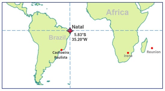
Figure 1.
Geographical position of the study site of Natal in the north of Brazil (the red star symbol), an equatorial location (5.4°S, 35.4°W) operated by the INPE (National Institute for Space Research), Brazil. Cachoeira (22.68°S, 45.00°W), Irene (25.90°S, 28.22°E), and Reunion (20.89°S, 55.53°E) sites are indicated by red dots.
2.1.1. Satellite Observations: TOMS, OMI, MLS-OMI
For this study, ozone measurements from satellites were used and combined with ground-based observations at Natal. Satellite data are from the Total Ozone Mapping Spectrometer (TOMS) on board the Earth-Probe Total satellite, and from the Ozone Monitoring Instrument (OMI) and Microwave Limb Sounder (MLS) instruments on the Aura satellite. TOMS is a spectrometer with nadir viewing, with vertical and horizontal resolutions of 77 km and 50 km × 50 km, respectively. Its method of ozone retrieval is based on the principle of differential absorption by ozone of the solar and Earth’s atmosphere backscatters directed towards the satellite within six discrete wavelengths [25]. TOMS data considered in the present work are from the V8 L3 product overpass for the Natal station over the period between 1998 and 2005. As for the OMI instrument, it is on board the Aura satellite launched in July 2004 with a near-polar helio-synchronous orbit. Like TOMS, OMI performs measurements through the backscatter ultraviolet technique. It has three broad spectral bands: UV-1 (270–310 nm), UV-2 (310–365 nm) and visible (350–500 nm), with a spectral resolution of the order of 0.5 nm [25]. The OMI and TOMS total columns of ozone have a precision of about 3%, and they exhibit good agreement with ground-based measurements (Dobson and SAOZ) across the southern tropics and subtropics [15]. TCO from OMI passes over Natal, from August 2004 to December 2019, were used together with TCO from TOMS to cover the whole study period (from January 1998 to December 2019).
Regarding the tropospheric partial column of ozone (Trop-CO) time series from the satellite, we used the Trop-CO product retrieved by combining OMI and MLS observations recorded between August 2004 and December 2019. MLS is a nadir-viewing instrument that produces around 3500 vertical profiles of temperature, ozone, and other chemical trace gases every day from the troposphere up to the mesosphere. It does this by monitoring microwave radiation from the Earth’s limb in the forward direction of the Aura orbit [26]. Daily Trop-CO values were obtained through the method developed by Ziemke et al. (2006) [27]. They used the tropospheric ozone residual method, which consists of subtracting measurements of MLS stratospheric column ozone from OMI total column ozone, to derive global distributions of tropospheric column ozone, which are then spatially interpolated each day to fill in the gaps between the actual along-track measurements; monthly mean fields are calculated by averaging all available daily data within each month. In their findings, Ziemke et al. (2006) reported that there were no significant calibration differences for tropospheric ozone measurements between the tropics and high latitudes when comparing OMI and MLS ozone inversions [27]. However, they did find persistent differences of 10 DU in the tropics, specifically from June to October over North Africa and extending westwards to the Atlantic. This feature coincides with the season of sandstorms originating in the northern African Sahara Desert, but it does not seem to affect the Natal site.
2.1.2. Radiosonde Data
As for most SHADOZ sites, balloon measurements in Natal are carried out weekly. Indeed, the number of launches can reach 4 per month. During the study period from 1998 to 2019, 633 profiles were recorded. An ozone-sonde experiment is based on the use of an electrochemical cell (ECC) device, in addition to temperature, humidity, and pressure sensors in the radiosonde. The ozone abundance is measured in partial pressure as a profile from the surface to the altitude where the balloon explosion happens, which is between 26 and 35 km. During the ascent of the balloon-sonde, data are recorded at 2 s intervals and are subsequently averaged over 100-meter-height intervals. The balloon-sonde is generally launched at 13.00 UTC, which corresponds to 10.00 local time in Brazil, and the precisions of SHADOZ measurements have been evaluated to be ~5% [13]. For further information on the validation of the ECC ozone sensor instrument, the operating mode and algorithm used for data inversion, and the quality assessment of the ozone sensor, the reader is referred to the articles by Witte et al. (2017, 2018) [13,28], and by Thompson et al. (2017, 2019) [29,30]. The SHADOZ data used in this study was downloaded from the SHADOZ website (http://croc.gsfc.nasa.gov/shadoz, accessed on 22 December 2023).
2.1.3. Dobson Spectrometer Observations
The TCO is measured daily at Natal using a Dobson spectrophotometer. Its measurement principle is based on comparing the relative intensity of selected UV wavelength pairings from the sun or moon. Thus, the quantity of ozone present in a vertical column of air stretching from the ground to the top of the atmosphere can be determined by measuring the relative intensities of selected wavelength pairs. The result represents the observed ozone layer thickness at normal temperature and pressure and is given in Dobson Units (DU) [31]. The Dobson measurements are processed to obtain average daily TCO values using software originally developed by Stanek (2007) [32].
There are currently between 60 and 70 Dobson spectrometers in operation around the world. They form the primary ground-based ozone observation network. In Brazil, two Dobson spectrometers have been operational. The oldest one is the Dobson #114, which has been working at Cachoeira Paulista (22.68°S, 45.00°W) since 1976 (see Figure 1), while the Dobson #093 was installed in Natal 2 years later. There is also a network of Brewer spectrometers in Brazil at 5 locations distributed from the Equator to the South Pole (Natal, Cuiabá, Cachoeira Paulista, Santa Maria, and Brazilian Antarctica station) also dedicated to continuously monitoring ozone in the framework of an INPE-NASA long-term collaboration program. The ozone measurement program in Brazil is operated by the INPE, in association with research groups from local universities. This is especially the case in Natal where INPE and the Universidade Federal do Rio Grande do Norte (UFRN) have been coordinating ozone measurements using Dobson and Brewer spectrometers since 1985 in Natal [33]. The Dobson’s calibration is regularly checked and remains stable to within 1% of the world-standard reference instruments hosted by NOAA in the United States and the European-standard instrument operated by Deutscher Wetterdienst in Germany. The traceability of the calibration of the Dobson network is continually updated by the ad-hoc Dobson committee and can be consulted at this link http://www.o3soft.eu/dobsonweb/welcome.html (accessed on 22 December 2023). The Natal spectrophotometer was calibrated in 2010 and 2019.
Many studies that examined ozone trends used the total atmospheric columns of ozone, but it is important to assess ozone separately in the troposphere and the stratosphere. In this study, we have used radiosonde ozone profiles and daily TCO measurements to evaluate the variability and changes of both tropospheric and stratospheric ozone separately, as different modes of variability that contribute to their generation do not necessarily drive them to the same degree and therefore may not lead to the same trend. In this study, the time series for TCO, Trop-CO, and Strat-CO were derived by combining radiosonde ozone profiles and daily TCO observations recorded by the co-located Dobson spectrometer [18], over the 1998–2019 period. Like the method used by Bencherif et al. (2020b) [19], the tropospheric column was computed from balloon-sonde ozone profiles between ground and the lapse rate tropopause (LRT) height. In contrast, the stratospheric column was obtained by differentiating between TCO and Trop-CO, respectively, obtained from Dobson and balloon-sonde, and assuming that ozone concentration is negligible in the mesosphere. The missing ozone data in the ground-based records were completed from satellite observations from TOMS and OMI for the TCO time series and from MLS-OMI for the Trop-CO times series. By using this method, it was possible to generate three distinct ozone time series: total, tropospheric, and stratospheric columns of ozone. Figure 2 shows the monthly variations of the TCO, Trop-CO, and Strat-CO ground-based time series, superimposed with those from satellite records, TOMS, and OMI for TCO, and with MLS-OMI for Trop-CO.
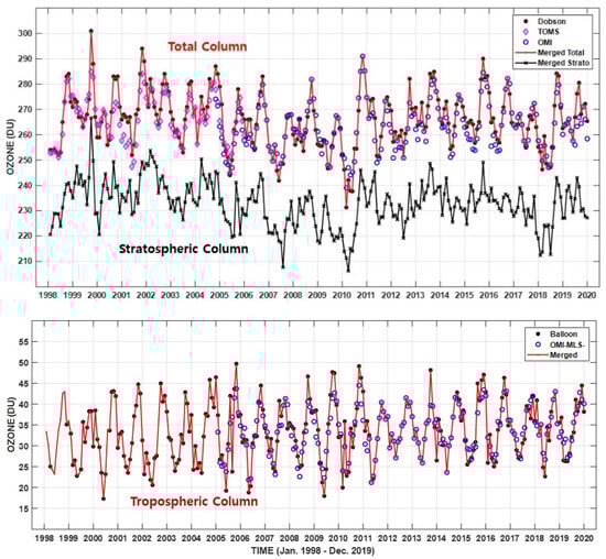
Figure 2.
Monthly time-series of total, stratospheric (upper panel) and tropospheric (lower panel) columns of ozone at Natal (5.40°S, 35.40°W), Rio Grande do Norte state, Brazil, obtained by combining and merging ground-based measurements (balloon-sonde profiles and Dobson total columns) and satellite observations from TOMS (until 2005), OMI, and OMI–MLS (see the legend). The merged ozone time series are shown with continuous lines.
The lower panel of Figure 2 depicts the Trop-CO monthly values obtained from balloon-sonde profiles (red line and black dots) together with the MLS-OMI values (blue symbols). The correlation between MLS-OMI and ozone sonde is high (0.79), whereas the relative difference is low at less than ±8%. The Trop-CO time series was constructed from radiosonde data and, when radiosonde experiments could not be performed, the gaps were filled by OMI-MLS values. Regarding the TCO time series, it was constructed based on monthly averaged TCO as derived from Dobson measurements, and completed by TOMS and OMI values when there is a gap in data. Figure 2 shows the monthly mean TCO values, with good agreement between ground-based (Dobson) and satellite (TOMS/OMI) data, a high correlation coefficient (of the order of 0.80) and minor differences, in agreement with the findings reported by Sousa et al. (2020) [18]. As described above, the Strat-CO time series was deduced by subtracting Trop-CO from TCO and assuming that ozone abundance is insignificant in the mesosphere. It is displayed with the black line on the same graph as TCO and shows almost the same fluctuations as TCO. This is expected since stratospheric ozone accounts for ≈90% of total ozone.
This paper aims to investigate ozone time series (TCO, Trop-CO, and Strat-CO) recorded at Natal, using the Empirical Adaptive Wavelet Decomposition (EAWD) algorithm developed by Delage et al. (2022) [22]. There are many numerical methods available to process a signal in terms of variability and trend estimate. The following subsections give an overview of three numerical methods commonly used to investigate variability and trend in the field of atmospheric and climate science: the Multi-Linear Regression (MLR), the Empirical Modal Decomposition (EMD) and Empirical Wavelet Transform (EWT) methods.
2.2. The Multi-Regression Method: Trend-Run Model
The linear multi-regression method is the most common and the oldest used method for the analysis of the variability of many geophysical parameters. The Trend-Run model developed at Reunion University is based on the MLR method [16,17]. It has been successfully applied to several observation time series of meteorological and atmospheric parameters, including temperature and ozone [15,16]. The MLR method assumes prior knowledge of the forcings that may contribute to the studied signal. The principle of the MLR method is based on breaking down a signal x(t) into the sum of forcings that contribute to its variability, in addition to a trend component :
with representing the coefficient contribution of the forcing , and as the trend term which is parametrized as linear. Indeed, the MLR method requires prior knowledge of the prevalent forcings and assumes the trend to be linear. The method was applied to the Natal ozone time series, for comparison with the results from the EAWD method.
2.3. EMD and EWT Decomposition Methods
Several numerical methods have been developed to consider the non-linear and non-stationary behavior of a signal more effectively. Some of them are well-adapted and deserve to be extensively applied to meteorological, climate, and environmental data. Two methods have been increasingly used as both are particularly well suited to the non-stationary nature of the observational time series: the EMD developed by Huang et al. (1998) [20], and the EWT described by Gilles (2013) [21]. Unlike the MLR method, the EMD and EWT decomposition methods do not require prior knowledge of the forcings that contribute to the variations of the study signal. The EMD operates in the time domain and thus has the advantage of being driven by real data based on the observations and allows the extraction of the Intrinsic Mode Functions (IMF), in addition to the implicit trend:
where is the residual mode.
As explained by Huang et al. (1998) [20], the frequency content generated by the EMD is determined from the relative positions of the maxima of the original signal, which generates IMFs with close frequencies, sometimes difficult to resolve, leading to what is called mode-mixing [34]. Indeed, the EMD method has the advantage of being driven by real data and allows extraction of the significant IMFs, while its main limitation is the frequency resolution. In contrast, the EWT operates in the frequency domain, and it is applied to the Fourier transform spectrum of the original signal, which consists of building an ensemble of pass-band filters from the Fourier spectrum. As described by Gilles (2013) [21] and shown by Delage et al. (2022) [22], the EWT allows a better frequency resolution, and thus overcomes the phenomenon of mode-mixing, by partitioning the spectrum of the original signal into separate spectral bands. However, while the EWT allows relevant frequencies to be detected in the original signal x(t), it does not allow the frequencies detected to be linked to a mode of variability, as the EMD does.
2.4. EAWD Decomposition
In this paper, we used the recently developed EAWD decomposition method, which combines the advantages of both EMD and EWT approaches. The principle of EAWD is based on identifying the modes of variability in the analyzed signal, in the form of a sum of the most significant IMFs. When a mode (IMF) shows a low contribution (less than 1%), it is incorporated into the trend component, the residual mode. The selected IMFs are then used as frequency supports for the segmentation of the Fourier spectrum of the signal into spectral bands framing each IMF.
As detailed by Delage et al. (2022) [22], the Fourier spectrum segmentation process is based on the local maxima of the IMFs spectra provided by EMD and it is performed according to two criteria: (1) the spectrum of two consecutive IMFs ( and ) contains at most two different dominant frequencies; the frequency with the greatest spectral density is the dominant one; (2) the local peaks of the spectra of two consecutive IMFs are subdivided into three groups: the local peaks in the spectrum, the local peaks belonging to the intersection of the and spectra, and the local peaks in the spectrum. The following step consists of applying the EWT to the spectral bands of each IMF, which makes it possible to identify the different modes of variability separately, thus avoiding the occurrence of mode-mixing phenomena.
3. Results
To investigate variability and trends, we applied the EAWD method to the TCO, Strat-CO, and Trop-CO time series recorded at Natal. The results are compared with those obtained by the EMD and MLR methods in terms of identification and quantification of ozone variability modes and in terms of trend estimates.
Ozone Variability Modes by EMD and EAWD Methods
As depicted in Figure 3, 5 IMFs were retrieved by applying the EMD and EAWD algorithms on the Natal total ozone series (TCO). Indeed, in addition to the residual trend term, the two methods revealed five quasi-similar modes, free of mode-mixing. They are labelled IMFi, with the i variable between 1 and 5. Each IMF is associated with a mode of variability with a dominant frequency, and therefore with a period of oscillation. Figure 3f superimposes the spectral densities of the 5 IMFs, highlighting the separation into disjoint spectral bands, as achieved by the EAWD method. IMF1 and IMF2 have periods of 6 and 12 months, respectively, and can be associated with semi-annual and annual seasonal oscillations. The periods of IMF3 and IMF4 are of the order of 26 and 33 months (2.2 and 2.8 years). We associate them with the interannual variability of the QBO, which is discussed in this paper. As for the IMF5, it is characterized by a period of 133 months (~11 years). It is, therefore, associated with the 11-year solar cycle. As reported by Delage et al. (2022) [22], the EAWD decomposition method allows the estimation of the percentage contribution of the detected modes (IMFs) to the variability of the studied signal. For the TCO Natal series, the total contribution of the modes identified (semi-annual, annual, QBO and solar) is 92.4%, of which 40.9% is associated with the annual cycle and 20.6% with the semi-annual cycle. As for the residual term, it is associated with the trend profile of the TCO over the study period. It is discussed in the next subsection. The application of the EAWD algorithm to the tropospheric and stratospheric ozone time series revealed the occurrence of a 3-month mode in both signals. The obtained results are summarized in Table 1.
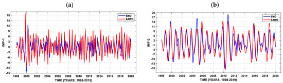
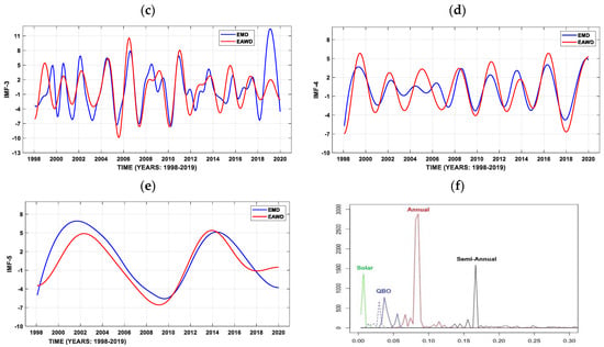
Figure 3.
(a) IMF1, (b) IMF2, (c) IMF3, (d) IMF4, and (e) IMF5, as detected by the EMD (blue line) and EAWD (red line) algorithms applied the TCO at Natal over the 1998–2019 period of observation. Plot (f) superimposes their spectral densities.

Table 1.
The cells indicate the percentage contributions of the ozone variability modes as revealed by the EAWD algorithm when applied to TCO, Trop-CO, and Strat-CO time series obtained at Natal, Brazil, over the 1998–2019 period. The last line summarizes the estimated trends for the three ozone time series.
The application of EMD and EAWD algorithms to the stratospheric ozone column (Strat-CO) revealed five modes with periods of 3, 6, 26, 33, and 133 months, with a total contribution of 89.5%. As for the results obtained for the tropospheric ozone column (Trop-CO), both methods allowed the detection of three modes (with contributions higher than 3%) with periods of 3, 6, and 12 months, and a total contribution of 95.4%. Overall, regardless of the time series, the EAWD method appeared to be effective and permitted the recovery of ~90% to 95% of ozone variability. Taking into account the Residu mode, which is associated with the trend over the observation period, it was found that the average difference between the original signal (e.g., Strat-CO) and the one reconstructed by summing the EAWD IMFs (), is very small (ΔStrat-CO = 0.0049 DU). The identified forcings are consistent with the findings of earlier studies on ozone variability in the tropics. Toihir et al. (2018) [15] analyzed the variability and trends of ozone from radiosonde data collected at 8 SHADOZ stations, including the Natal site, over the 1998–2012 period. They showed that ~80% of total ozone variability is due to the semi-annual, annual, QBO, and solar forcings. More recently, by combining ground-based and satellite TCO measurements at Cachoeira Paulista and Natal, Brazil, from early 1970 to 2013, Sousa et al. (2020) [18] reported the presence of the annual cycle at both sites.
One of the remarkable results of the EAWD decomposition is the identification of a 3-month mode in both tropospheric and stratospheric ozone time series. This mode can be associated with the Madden–Julian oscillation (MJO). The MJO is a large-scale coupling between atmospheric circulation and tropical deep-atmospheric convection. It is the most important mode of inter-seasonal variability in the tropical atmosphere. It is characterized by a periodicity between 30 and 90 days [35] and exerts an influence on tropospheric ozone [36] and on stratospheric ozone [37]. Indeed, it can be deduced that the separation between tropospheric and stratospheric ozone columns and the application of the EAWD algorithm revealed the presence of the 3-month MJO, with a higher contribution in the troposphere (15.8%) than in the stratosphere (11.9%) (see Table 1). Regarding the semi-annual mode (6-month period), it is present in both ozone time series. However, its contribution to stratospheric ozone variability is more significant (17.6%), with nearly double the contribution to tropospheric ozone variability (8.8%). As for the annual cycle (12-month period), it appears to be the dominant forcing in the variability of tropospheric ozone (69%), while it shows no contribution to the variability of the stratospheric ozone. These results on seasonal modes are consistent with those published. Bencherif et al. (2006) [16] found similar results using a temperature time series recorded over the southern tropics (South Africa). Indeed, they performed a Fourier analysis at different heights on temperature distributions recorded over the 1980–2001 period in the UT-LS region and highlighted two dominant seasonal oscillations: annual and semi-annual modes. Moreover, Toihir et al. (2018) [15] showed that, for equatorial stations, the contribution of the annual mode is dominant in the tropospheric ozone (where it explains nearly 70% of ozone variability), and weaker in the stratospheric ozone; while the semi-annual mode shows inverse contributions: strong contribution in the stratosphere (~30%) and a weak contribution in the troposphere (<5%). As far as the QBO mode is concerned, it can be recalled beforehand that it is a quasi-periodic forcing that dominates the tropical stratosphere. It is characterized by a regular change in the zonal wind over the equator, a downward propagation, and a variable period between 24 and 30 months [38]. The QBO leads to anomalies in the mean meridional flow and consequently affects the concentrations of chemical compounds, including ozone. From Figure 3c,d above, together with Table 1, the EMD and EAWD methods revealed two IMFs with periods of 26 and 33 months in the stratospheric ozone time series, which we associated with the QBO forcing. This suggests that the EMD and EAWD decomposition methods are not able to detect modes with changing periodicity, which is the case for the QBO. Nevertheless, as can be seen in Figure 4, the summing up of QBO1 (IMF3) and QBO2 (IMF4) (26- and 33-month period modes) results in a signal that is highly correlated with the zonal wind at 20 hPa over Singapore (correlation coefficient rstrat = 0.75). It should be emphasized that the stratospheric zonal wind observed in Singapore (1°N, 104°E) is usually used as a QBO index. This shows that some forcings could be derived by combining the obtained IMFs from EAWD decompositions and confirms that the QBO is the mode contributing most to the variability of stratospheric ozone over Natal (39.1%).
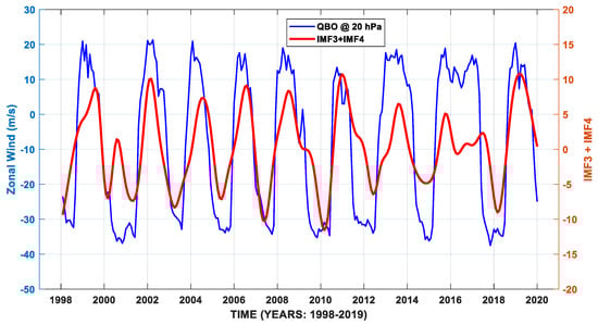
Figure 4.
Zonal wind at the 20 hPa pressure level over Singapore (1°N, 104°E), corresponding to the QBO index (blue line), superimposed on the sum of IMF3 and IMF4 standing respectively for QBO1 and QBO2, and periods of 26 and 33 months (red line) over the study period from 1998 to 2019.
Regarding the solar cycle forcing, it corresponds to a nearly periodic 11-year change in the solar activity. It is associated, in the present work, with the IMF5, which has a period of 133 months (~11 years) (see Figure 3f) and makes an important contribution to the variability of stratospheric ozone (18%). It also has a high correlation with the solar flux at 10.7 cm (r = 0.53/rstrat = 0.74). The latter is usually used to parametrize the solar cycle [16].
4. Discussion
Trend Estimates by MLR and EAWD
As stated above, the key difference between the MLR method and the EAWD algorithm lies in the way that the forcing modes of the study signal are defined or detected. The MLR method requires prior knowledge of the forcing modes, while the EAWD operates without this. For both methods, the inherent trend in the signal is given by the residual term. Figure 5 shows the time series together with trend results obtained by applying the MLR and EAWD methods to the three ozone time series of the present study (i.e., TCO, Trop-CO, and Strat-CO). For the TCO (Figure 5a), both methods showed a decrease in total ozone over the observation period. Due to its principle, based on a multi-linear regression, the MLR trend is linear. It is represented here as a straight line with a negative slope, which corresponds to a decreasing trend in the order of −0.60 ± 0.30% (−1.6 DU/decade). This result agrees with the one published by Sousa et al. (2020) [18], who analyzed TCO trends by combining Dobson and satellite observations over two Brazilian sites, Cachoeira Paulista and Natal, and found a negative trend in TCO at Natal over the 1978–2013 period, of the order of −0.78%.
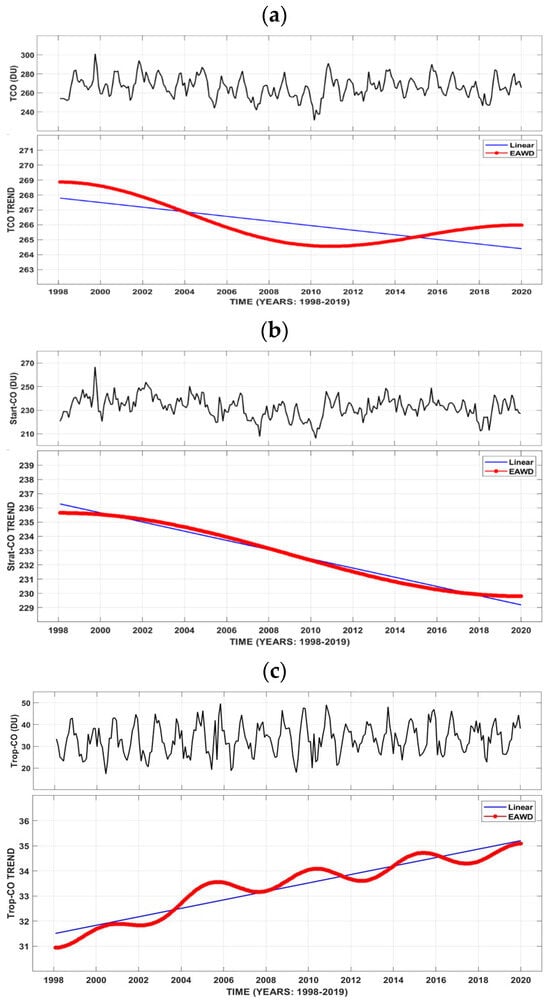
Figure 5.
Ozone time series and trend curves as derived from the MLR and EAWD methods for (a) TCO, (b) Strat–CO, and (c) Trop–CO, respectively, in blue and red lines, from 1998 to 2019.
However, it must be noted that the trend curve obtained by the EAWD method (solid red line, Figure 5a) does not show the same variation as the MLR trend. It shows two broad phases, one decreasing between 1998 and 2011, and another one increasing from 2011 to 2019. This gives the EAWD method the advantage of detecting possible breakpoint in the trend, which seems to appear here by 2011 for total ozone at Natal.
As for the tropospheric and stratospheric ozone time series (Trop-CO and Strat-CO), the MLR and EAWD methods showed almost similar trends, which are a decrease in the stratosphere ozone (−3.2 DU/decade, −1.3 ± 0.8%) and an increase in the tropospheric ozone (+1.7 DU/decade, +4.9 ± 1.3%). This agrees with results reported in recent studies [18,20]. In the latter work, based on radiosonde ozone profiles from SHADOZ stations located in the equatorial region (5.6°N–14°S), including Natal, the authors found that ozone increased in the free troposphere (~(1–4)% per decade) but decreased in the lowermost stratospheric ozone, i.e., ~(−3)% per decade over the 1998–2019 period. Bencherif et al. (2020b) [19] combined ground and satellite observations to analyze the ozone time series at Irene (25.90°S, 28.22°E), South Africa, over the 1998–2017 period. They applied the Trend-Run model (based on the MLR method) and the Mann–Kendall (MK) test, for trend analysis. In fact, they also showed a decrease in the stratospheric ozone (−0.56% and −1.7% per decade using MLR and MK methods, respectively), but an increase in the tropospheric ozone (+2.37% and +3.6% per decade from MLR and MK, respectively). In comparison with the Irene site, the relatively high increasing trend of tropospheric ozone at Natal may be related to an increase in emissions of ozone precursors. Furthermore, as reported by Clain et al. (2009) [39] and by Thompson et al. (2014) [6], the increase in tropospheric ozone can be associated with increases in anthropic activities (urbanization, transport, industrialization) and in biomass burning, and, on a larger scale, it can be associated with the long-range transport of increasing pollution in the Southern Hemisphere. This agrees with the finding from Kim and Newchurch (1998) [24]. In their work, they investigated the influences of biomass burning on tropospheric ozone over Natal using radiosonde data. They reported that the annual maximum of ozone observed during spring (September–November) is related to the increase in biomass-burning activity. Kim and Newchurch (1998) [24] also found, from their statistical analysis applied to 22 years of back-trajectory simulations, that during the fire season, Natal is underneath long-range ozone transport mainly originating from Africa across the Atlantic Ocean (in ~80% of cases) in the 1–6 km altitude range.
The observed decrease in stratospheric ozone over Natal is in line with global circulation model simulations. These simulations showed that the BDC is predicted to be accelerating over the next century [40], leading to a decrease in ozone in the tropics and to an increase at higher latitudes [41]. In addition, Quang Fu et al. (2019) [42] used satellite MSU/AMSU observations and ERA-Interim reanalysis datasets to examine the BDC changes for the 1980–2018 period. They showed that the annual average BDC has accelerated over the past 40 years with a relative strengthening of ~1.7% per decade.
5. Conclusions
This study aimed to gain a better understanding of ozone variability and trend estimates at Natal, an equatorial site in northern Brazil, using traditional multi-linear regression compared with empirical decomposition methods. We examined the capabilities of the new EAWD decomposition method developed by Delage et al. (2022) [22] when applied to ozone time series. The data we used included total columns of ozone together with tropospheric and stratospheric partial columns, derived by combining ozone profiles and total columns of ozone recorded by balloon-sonde and Dobson measurements at the study site. The ozone time series obtained showed good agreement with the satellite products (see Figure 2), which highlights the advantage of combining these products to create a homogeneous ozone time series for studying ozone variability and trends. Our study emphasizes the importance of combining data to analyze the variability and trend of tropospheric and stratospheric ozone separately. It is recommended, therefore, to analyze the variability and trends of ozone by examining the tropospheric and stratospheric components separately, whenever possible. This is because the different modes of variability that contribute to their generation do not necessarily drive them to the same degree and so may not lead to the same trend.
For the Natal TCO dataset, we identified five modes associated with semi-annual, annual, QBO1, QBO2, and solar forcings accounting for 92.4% of total ozone variability, of which 40.9% was found to be due to the annual cycle and 20.6% to the semi-annual cycle. One of the remarkable results from the EAWD decomposition is the identification of a 3-month mode in both tropospheric and stratospheric ozone time series, while it does not appear in the TCO data. This mode is associated with the MJO forcing. The annual mode appeared to strongly drive the variability of tropospheric ozone, with a contribution equal to 69%, while it made no contribution to the variability of the stratospheric ozone (see Table 1).
Unexpectedly, the EAWD decompositions revealed 2 QBO components, QBO1 and QBO2, in total and stratospheric columns of ozone, which highlights a limitation of this algorithm in detecting modes with changing periodicity, which is the case for the QBO. However, the combination of QBO1 and QBO2 allowed us to retrieve the QBO mode, with a high contribution to stratospheric ozone variability (39.1%).
In addition to the variability analysis, this study compares ozone trends obtained by the MLR and EAWD methods.
As previously reported by Delage et al. (2022) [22], the EAWD method confirmed the advantage of detecting possible breakpoints in the trend, which appeared here in 2011 for total ozone at Natal. Regarding trend analyzes and estimates, the MLR and EAWD methods showed almost similar trends, namely a decrease in the stratospheric ozone (−1.21%) and an increase in the tropospheric ozone (+0.64%).
However, it should be emphasized that the EAWD method is still under development and needs to be improved to make it automatic, especially in the Fourier spectrum segmentation process. This requires manual control to ensure no overlap between the spectral bands framing each mode (IMF). In addition, it is important to be cautious when interpreting the modes of variability obtained, particularly when they have a variable periodicity, such as the QBO or the ENSO (El Niño Southern Oscillation).
Author Contributions
Conceptualization, H.B. and D.K.P.; methodology, H.B. and O.D.; software, O.D. and T.M.; validation, H.B. and N.B.; formal analysis, H.B.; investigation, H.B.; resources, M.P.P.M.; data curation, H.B. and F.R.d.S.; writing—original draft preparation, H.B.; writing, review and editing, all authors; project administration and funding acquisition, H.B. and D.K.P. All authors have read and agreed to the published version of the manuscript.
Funding
This research was funded by the French-Brazilian CAPES-COFECUB program for supporting research activities under the AEROBI (AERosol Observations over Brazil and Impacts) project, process n. COFECUB-20222232369P, and CAPES n. 88887.711959/2022-00. The APC was funded by Université de la Réunion and CNRS.
Acknowledgments
The authors are thankful to the International Office (Direction des Relations Internationales) of Reunion University for travel support and assistance with the implementation of the agreements between the partners. The authors thank the SHADOZ, WOUDC, and NASA teams for archiving and providing ozone data.
Conflicts of Interest
The authors declare no conflicts of interest.
References
- Fountoulakis, I.; Diémoz, H.; Siani, A.-M.; Laschewski, G.; Filippa, G.; Arola, A.; Bais, A.F.; De Backer, H.; Lakkala, K.; Webb, A.R.; et al. Solar UV Irradiance in a Changing Climate: Trends in Europe and the Significance of Spectral Monitoring in Italy. Environments 2019, 7, 1. [Google Scholar] [CrossRef]
- van der Werf, G.R.; Randerson, J.T.; Giglio, L.; van Leeuwen, T.T.; Chen, Y.; Rogers, B.M.; Mu, M.; van Marle, M.J.E.; Morton, D.C.; Collatz, G.J.; et al. Global fire emissions estimates during 1997–2016. Earth Syst. Sci. Data 2017, 9, 697–720. [Google Scholar] [CrossRef]
- Bertschi, I.T.; Jaffe, D.A.; Jaeglé, L.; Price, H.U.; Dennison, J.B. PHOBEA/ITCT 2002 airborne observations of transpacific transport of ozone, CO, volatile organic compounds, and aerosols to the northeast Pacific: Impacts of Asian anthropogenic and Siberian boreal fire emissions. J. Geophys. Res. 2004, 109, D23S12. [Google Scholar] [CrossRef]
- Clerbaux, C.; Boynard, A.; Clarisse, L.; George, M.; Hadji-Lazaro, J.; Herbin, H.; Hurtmans, D.; Pommier, M.; Razavi, A.; Turquety, S.; et al. Monitoring of atmospheric composition using the thermal infrared IASI/MetOp sounder. Atmos. Chem. Phys. 2009, 9, 6041–6054. [Google Scholar] [CrossRef]
- Duflot, V.; Dils, B.; Baray, J.L.; de Maziere, M.; Attié, J.-L.; Vanhaelewyn, G.; Senten, C.; Vigouroux, C.; Clain, G.; Robert, D. Analysis of the origin of the distribution of CO in the subtropical southern Indian Ocean in 2007. J. Geophys. Res. 2010, 115, D22106. [Google Scholar] [CrossRef]
- Thompson, A.M.; Balashov, N.V.; Witte, J.C.; Coetzee, J.G.R.; Thouret, V.; Posny, F. Tropospheric ozone increases over the southern Africa region: Bellwether for rapid growth in Southern Hemisphere pollution? Atmos. Chem. Phys. 2014, 14, 9855–9869. [Google Scholar] [CrossRef]
- Torres, O.; Tanskanen, A.; Veihelmann, B.; Ahn, C.; Braak, R.; Bhartia, P.K.; Veefkind, P.; Levelt, P.P. Aerosols and surface UV products from Ozone Monitoring Instrument observations: An overview. J. Geophys. Res. Space Phys. 2007, 112. [Google Scholar] [CrossRef]
- Bencherif, H.; Bègue, N.; Kirsch Pinheiro, D.; du Preez, D.J.; Cadet, J.-M.; da Silva Lopes, F.J.; Shikwambana, L.; Landulfo, E.; Vescovini, T.; Labuschagne, C.; et al. Investigating the Long-Range Transport of Aerosol Plumes Following the Amazon Fires (August 2019): A Multi-Instrumental Approach from Ground-Based and Satellite Observations. Remote Sens. 2020, 12, 3846. [Google Scholar] [CrossRef]
- du Preez, D.J.; Bencherif, H.; Portafaix, T.; Lamy, K.; Wright, C.Y. Solar Ultraviolet Radiation in Pretoria and Its Relations to Aerosols and Tropospheric Ozone during the Biomass Burning Season. Atmosphere 2021, 12, 132. [Google Scholar] [CrossRef]
- Bègue, N.; Bencherif, H.; Jégou, F.; Vérèmes, H.; Khaykin, S.; Krysztofiak, G.; Portafaix, T.; Duflot, V.; Baron, A.; Berthet, G.; et al. Transport and Variability of Tropospheric Ozone over Oceania and Southern Pacific during the 2019–20 Australian Bushfires. Remote Sens. 2021, 13, 3092. [Google Scholar] [CrossRef]
- Khaykin, S.; Legras, B.; Bucci, S.; Sellitto, P.; Isaksen, L.; Tencé, F.; Bekki, S.; Bourassa, A.; Rieger, L.; Zawada, D.; et al. The 2019/20 Australian wildfires generated a persistent smoke-charged vortex rising up to 35 km altitude. Commun. Earth Environ. 2020, 1, 22. [Google Scholar] [CrossRef]
- Thompson, A.M.; Witte, J.C.; McPeters, R.D.; Oltmans, S.J.; Schmidlin, F.J.; Logan, J.A.; Fujiwara, M.; Kirchhoff, V.W.; Posny, F.; Coetzee, G.J.; et al. Southern Hemisphere Additional Ozonesondes (SHADOZ) 1998–2000 tropical ozone climatology 1. Comparison with Total Ozone Mapping Spectrometer (TOMS) and ground-based measurements. J. Geophys. Res. Atmos. 2003, 108, 8238. [Google Scholar] [CrossRef]
- Witte, J.C.; Thompson, A.M.; Smit, H.G.; Fujiwara, M.; Posny, F.; Coetzee, G.J.; Northam, E.T.; Johnson, B.J.; Sterling, C.W.; Mohamad, M.; et al. First reprocessing of Southern Hemisphere ADditional OZonesondes (SHADOZ) profile records (1998–2015): 1. Methodology and evaluation. J. Geophys. Res. 2017, 122, 6611–6636. [Google Scholar] [CrossRef]
- Randel, W.J.; Thompson, A.M. Interannual variability and trends in tropical ozone derived from SAGE II satellite data and SHADOZ ozonesondes. J. Geophys. Res. 2011, 116, D07303. [Google Scholar] [CrossRef]
- Toihir, A.M.; Portafaix, T.; Sivakumar, V.; Bencherif, H.; Pazmiño, A.; Bègue, N. Variability and trend in ozone over the southern tropics and subtropics. Ann. Geophys. 2018, 36, 381–404. [Google Scholar] [CrossRef]
- Bencherif, H.; Diab, R.D.; Portafaix, T.; Morel, B.; Keckhut, P.; Moorgawa, A. Temperature climatology and trend estimates in the UTLS region as observed over a southern subtropical site, Durban, South Africa. Atmos. Chem. Phys. 2006, 6, 5121–5128. [Google Scholar] [CrossRef]
- Thompson, A.M.; Stauffer, R.M.; Wargan, K.; Witte, J.C.; Kollonige, D.E.; Ziemke, J.R. Regional and seasonal trends in tropical ozone from SHADOZ profiles: Reference for models and satellite products. J. Geophys. Res. 2021, 126, e2021JD034691. [Google Scholar] [CrossRef]
- Sousa, C.T.; Leme, N.M.P.; Martins, M.P.P.; Silva, F.R.; Penha, T.L.B.; Rodrigues, N.L.; Silva, E.L.; Hoelzemann, J.J. Ozone trends on equatorial and tropical regions of South America using Dobson spectrophotometer, TOMS and OMI satellites instruments. J. Atmos. Sol. Terr. Phys. 2020, 203, 105272. [Google Scholar] [CrossRef]
- Bencherif, H.; Toihir, A.M.; Mbatha, N.; Sivakumar, V.; du Preez, D.J.; Bègue, N.; Coetzee, G. Ozone Variability and Trend Estimates from 20-Years of Ground-Based and Satellite Observations at Irene Station, South Africa. Atmosphere 2020, 11, 1216. Available online: https://www.mdpi.com/2073-4433/11/11/1216 (accessed on 2 January 2024). [CrossRef]
- Huang, N.E.; Shen, Z.; Long, S.R.; Wu, M.C.; Shih, H.H.; Zheng, Q.; Yen, N.C.; Tung, C.C.; Liu, H.H. The empirical mode decomposition and the Hilbert spectrum for nonlinear and non-stationary time series analysis. Proc. R. Soc. London. Ser. A Math. Phys. Eng. Sci. 1998, 454, 903995. [Google Scholar] [CrossRef]
- Gilles, J. Empirical Wavelet Transform. IEEE Trans. Signal Process. 2013, 61, 3999–4010. [Google Scholar] [CrossRef]
- Delage, O.; Portafaix, T.; Bencherif, H.; Bourdier, A.; Lagracie, E. Empirical adaptive wavelet decomposition (EAWD): An adaptive decomposition for the variability analysis of observation time series in atmospheric science. Nonlin. Process. Geophys. 2022, 29, 265–277. [Google Scholar] [CrossRef]
- Thompson, A.M.; Witte, J.C.; Oltmans, S.J.; Schmidlin, F.J. SHADOZ—A tropical ozonesonde–radiosonde network for the atmospheric community. Bull. Am. Meteorol. Soc. 2004, 85, 1549–1564. [Google Scholar] [CrossRef]
- Kim, J.H.; Newchurch, M.J. Biomass-burning influence on tropospheric ozone over New Guinea and South America. J. Geophys. Res. 1998, 103, 1455–1461. [Google Scholar] [CrossRef]
- McPeters, R.D.; Bhartia, P.K.; Krueger, A.J.; Herman, J.R.; Wellemeyer, C.G.; Seftor, C.J.; Jaross, G.; Torres, O.; Moy, L.; Labow, G.; et al. Earth Probe Total Ozone Mapping Spectrometer (TOMS) Data Products User’s Guide; NASA, Goddard Space Flight Center: Greenbelt, MD, USA, 1998. [Google Scholar]
- Livesey, N.J.; Filipiak, M.J.; Froidevaux, L.; Read, W.G.; Lambert, A.; Santee, M.L.; Jiang, J.H.; Pumphrey, H.C.; Waters, J.W.; Cofield, R.E.; et al. Validation of Aura Microwave Limb Sounder O3 and CO observations in the upper troposphere and lower stratosphere. J. Geophys. Res. 2008, 113, D15S02. [Google Scholar] [CrossRef]
- Ziemke, J.R.; Chandra, S.; Duncan, B.N.; Froidevaux, L.; Bhartia, P.K.; Levelt, P.F.; Waters, J.W. Tropospheric ozone determined from Aura OMI and MLS: Evaluation of measurements and comparison with the Global Modeling Initiative’s Chemical Transport Model. J. Geophys. Res. 2006, 111, D19303. [Google Scholar] [CrossRef]
- Witte, J.C.; Thompson, A.M.; Smit, H.G.J.; Vömel, H.; Posny, F.; Stübi, R. First reprocessing of Southern Hemisphere ADditional OZonesondes profile records: 3. Uncertainty in ozone profile and total column. J. Geophys. Res. 2018, 123, 3243–3268. [Google Scholar] [CrossRef]
- Thompson, A.M.; Witte, J.C.; Sterling, C.; Jordan, A.; Johnson, B.J.; Oltmans, S.J.; Fujiwara, M.; Vömel, H.; Allaart, M.; Piters, A.; et al. First reprocessing of Southern Hemisphere Additional Ozonesondes (SHADOZ) ozone profiles (1998–2016): 2. Comparisons with satellites and ground-based instruments. J. Geophys. Res. 2017, 122, 13000–13025. [Google Scholar] [CrossRef]
- Thompson, A.M.; Smit, H.G.; Witte, J.C.; Stauffer, R.M.; Johnson, B.J.; Morris, G.; von Der Gathen, P.; Van Malderen, R.; Davies, J.; Piters, A.; et al. Ozonesonde Quality Assurance: The JOSIE–SHADOZ (2017) Experience. Bull. Am. Meteorol. Soc. 2019, 100, 155–171. [Google Scholar] [CrossRef]
- Komhyr, W.D. Operations Handbook—Ozone Observations with a Dobson Spectrophotometer. In WMO Global Ozone Research and Monitoring Project; Report No. 6; World Meteorological Organization: Geneva, Switzerland, 1980. [Google Scholar]
- Stanek, M. Total Ozone and UV Radiation Monitoring Software. 2007. Available online: http://www.o3soft.eu/ (accessed on 22 December 2023).
- Kirchhoff, V.W.J.H.; Barnes, R.A.; Torres, A.L. Ozone climatology at Natal, Brazil, from in situ ozonesonde data. J. Geophys. Res. 1991, 96, 10899–10909. [Google Scholar] [CrossRef]
- Fosso, O.B.; Molinas, M. Method for mode mixing separation in Empirical Mode decomposition. arXiv 2017, arXiv:1709.05547. [Google Scholar]
- Madden, R.A.; Julian, P.R. Observations of the 40–50 day tropical oscillation: A review. Mon. Weather Rev. 1994, 122, 814–837. [Google Scholar] [CrossRef]
- Ziemke, J.R.; Chandra, S. A Madden-Julian Oscillation in tropospheric ozone. Geophys. Res. Lett. 2003, 30, 2182. [Google Scholar] [CrossRef]
- Weare, B.C. Madden-Julian Oscillation in the tropical stratosphere. J. Geophys. Res. 2010, 115, D17113. [Google Scholar] [CrossRef]
- Baldwin, M.P.; Gray, L.J.; Dunkerton, T.J.; Hamilton, K.; Haynes, P.H.; Randel, W.J.; Holton, J.R.; Alexander, M.J.; Hirota, I.; Horinouchi, T.; et al. The quasi-biennial oscillation. Rev. Geophys. 2001, 39, 179–229. [Google Scholar] [CrossRef]
- Clain, G.; Baray, J.L.; Delmas, R.; Diab, R.; Leclair de Bellevue, J.; Keckhut, P.; Posny, F.; Metzger, J.M.; Cammas, J.P. Tropospheric ozone climatology at two Southern Hemisphere tropical/subtropical sites, (Reunion Island and Irene, South Africa) from ozonesondes, LIDAR, and in situ aircraft measurements. Atmos. Chem. Phys. 2009, 9, 1723–1734. [Google Scholar] [CrossRef]
- Butchart, N. The Brewer–Dobson circulation. Rev. Geophys. 2014, 52, 157–184. [Google Scholar] [CrossRef]
- Hegglin, M.I.; Shepherd, T.G. Large Climate-Induced Changes in Ultraviolet Index and Stratosphere-to-Troposphere Ozone Flux. Nat. Geosci. 2009, 2, 687–691. [Google Scholar] [CrossRef]
- Fu, Q.; Solomon, S.; Pahlavan, H.A.; Lin, P. Observed changes in Brewer–Dobson circulation for 1980–2018. Environ. Res. Lett. 2019, 14, 114026. [Google Scholar] [CrossRef]
Disclaimer/Publisher’s Note: The statements, opinions and data contained in all publications are solely those of the individual author(s) and contributor(s) and not of MDPI and/or the editor(s). MDPI and/or the editor(s) disclaim responsibility for any injury to people or property resulting from any ideas, methods, instructions or products referred to in the content. |
© 2024 by the authors. Licensee MDPI, Basel, Switzerland. This article is an open access article distributed under the terms and conditions of the Creative Commons Attribution (CC BY) license (https://creativecommons.org/licenses/by/4.0/).