


Investigating a Persistent Stratospheric Aerosol Layer Observed over Southern Europe during 2019
 , , , , and
Abstract
:1. Introduction
2. Instrumentation and Data Products
2.1. THEssaloniki LIdar SYStem (THELISYS)
Geometrical and Optical Retrievals with THELISYS
2.2. CALIPSO/CALIOP Observations and Aerosol Optical Properties and Typing Retrievals
2.3. Space-Borne OMPS-LP Aerosol Extinction Vertical Profiles
2.4. Stratospheric Composition Modelling
2.5. Summary of the Datasets Used in This Work
3. Results and Discussion
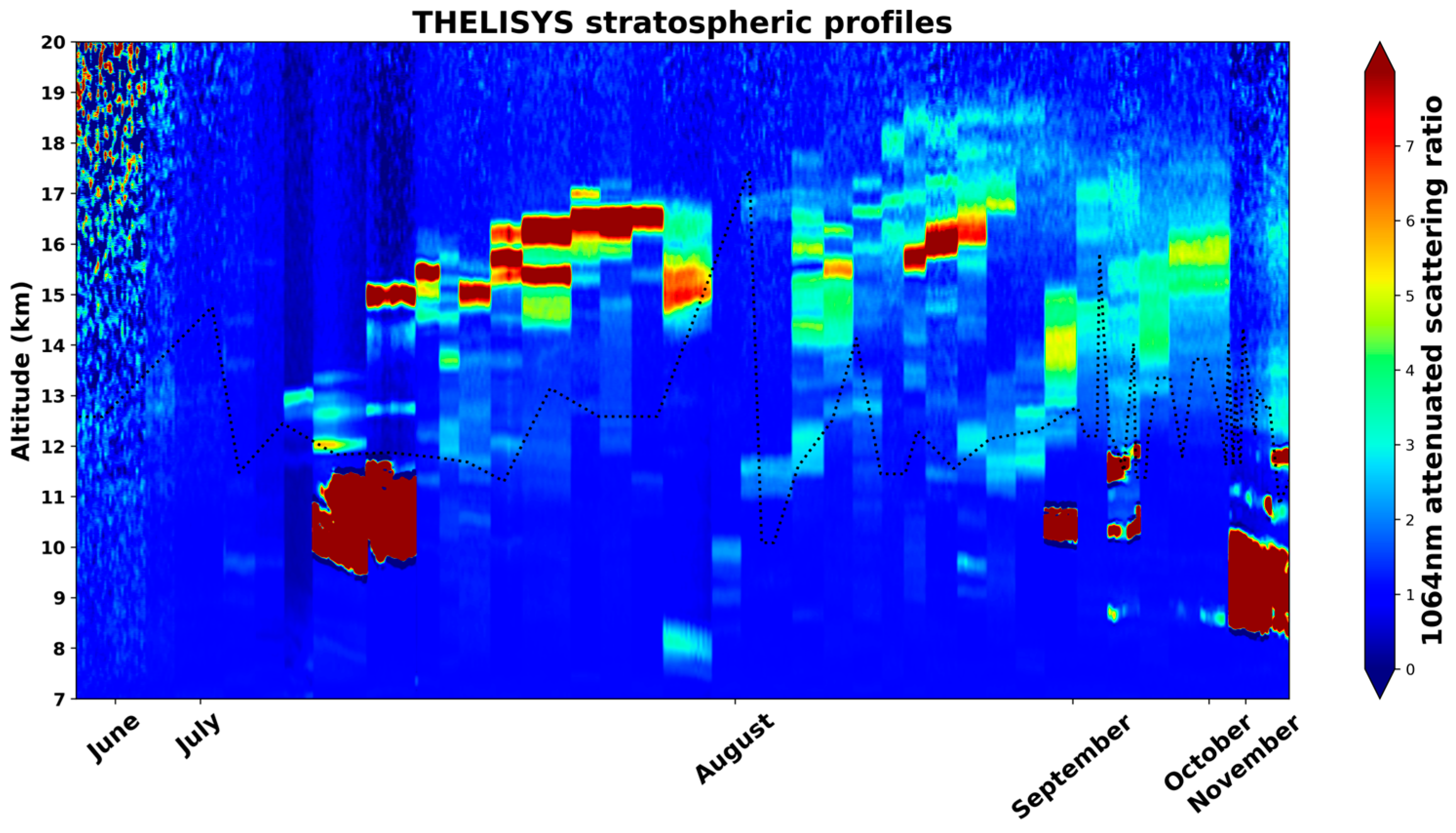
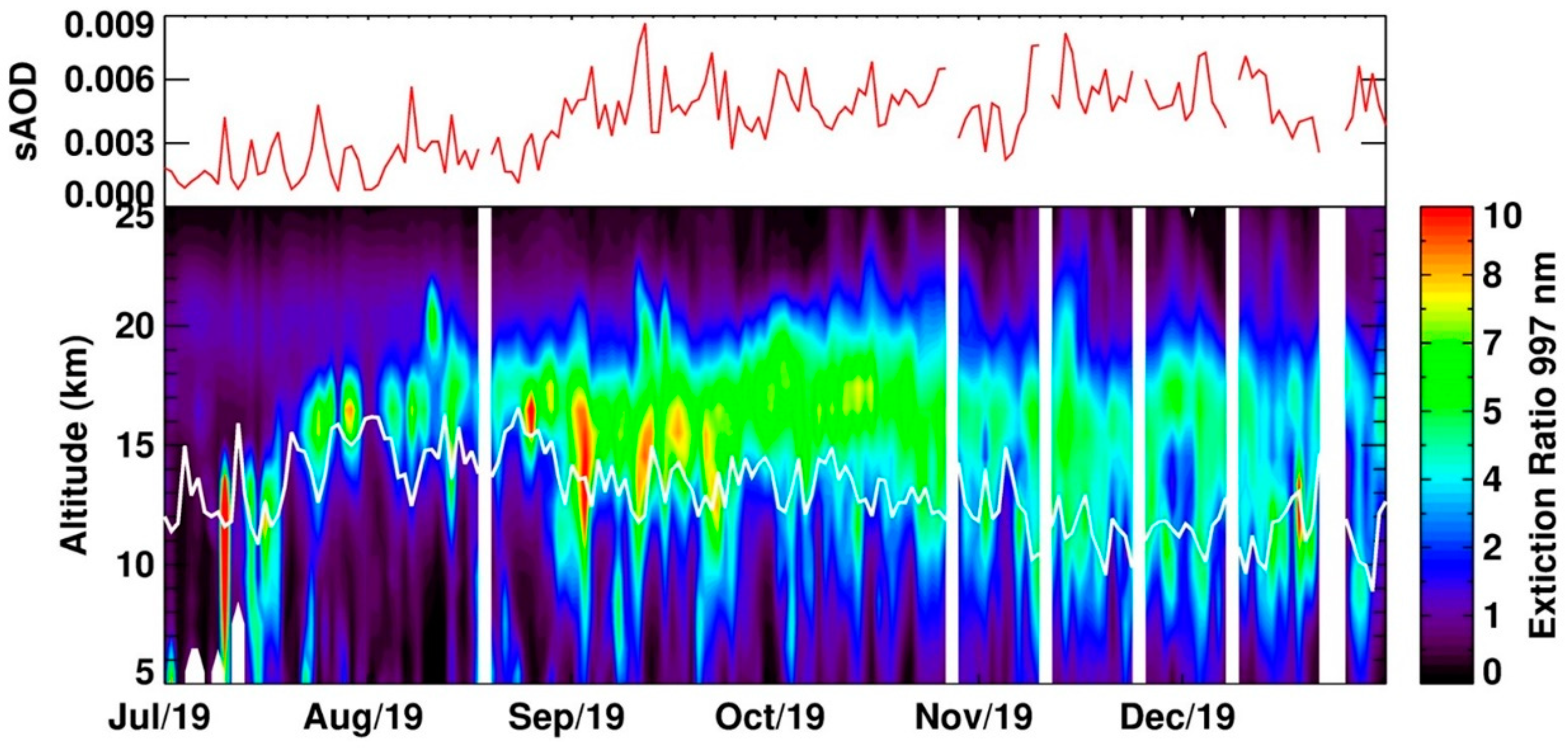
3.1. Temporal Evolution of the Stratospheric Layer
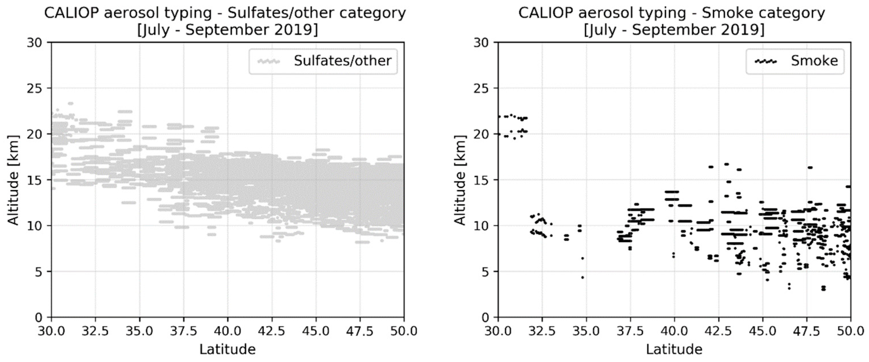
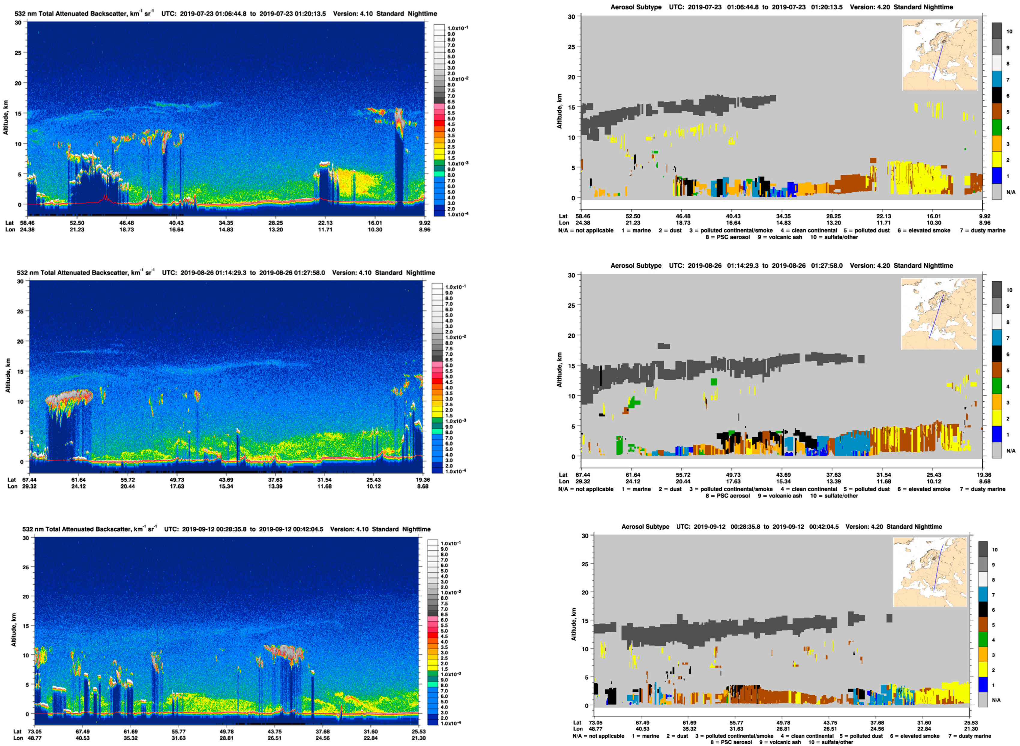
3.2. Identification of the Stratospheric Layer Origin Using CALIOP Aerosol Typing
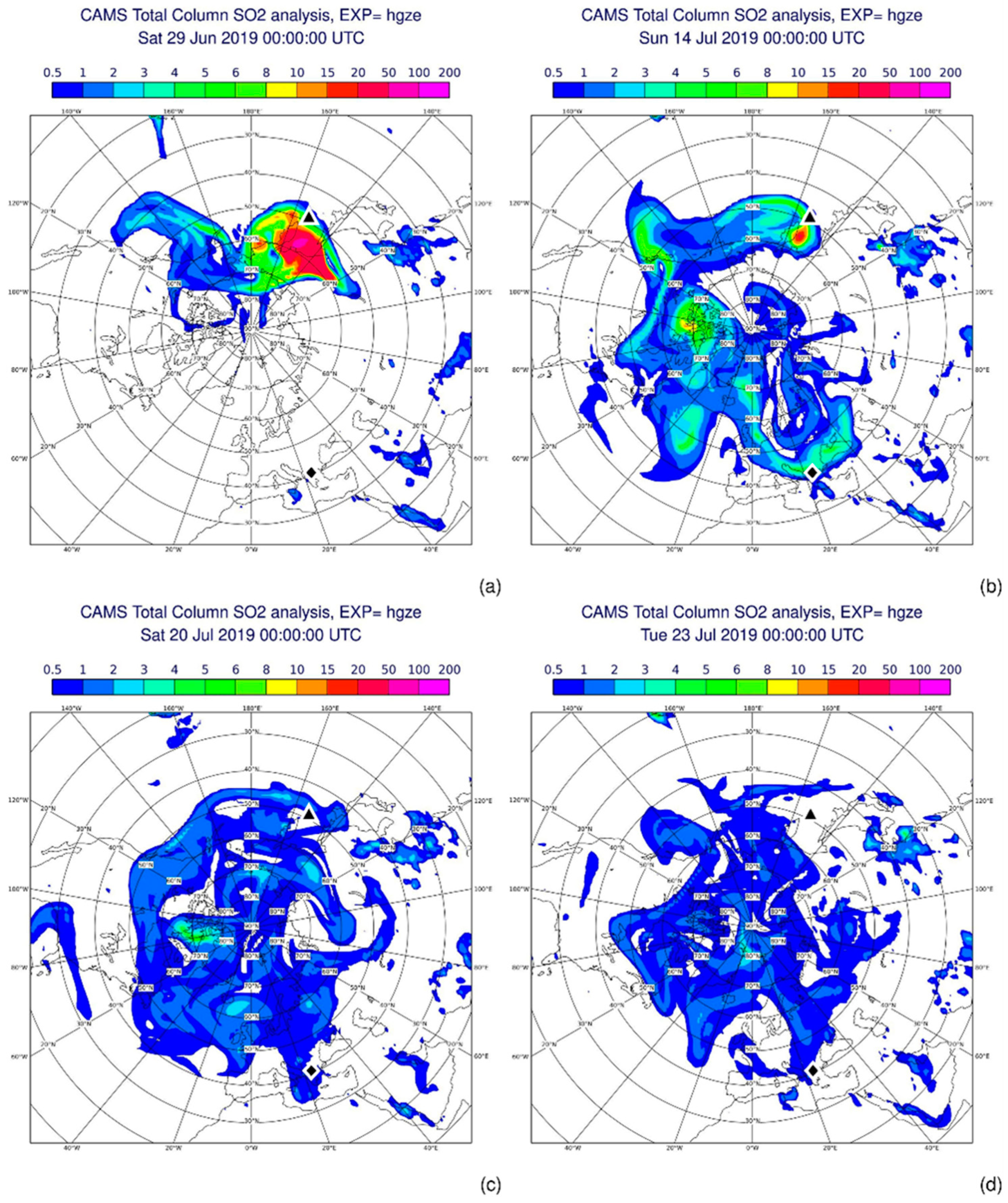
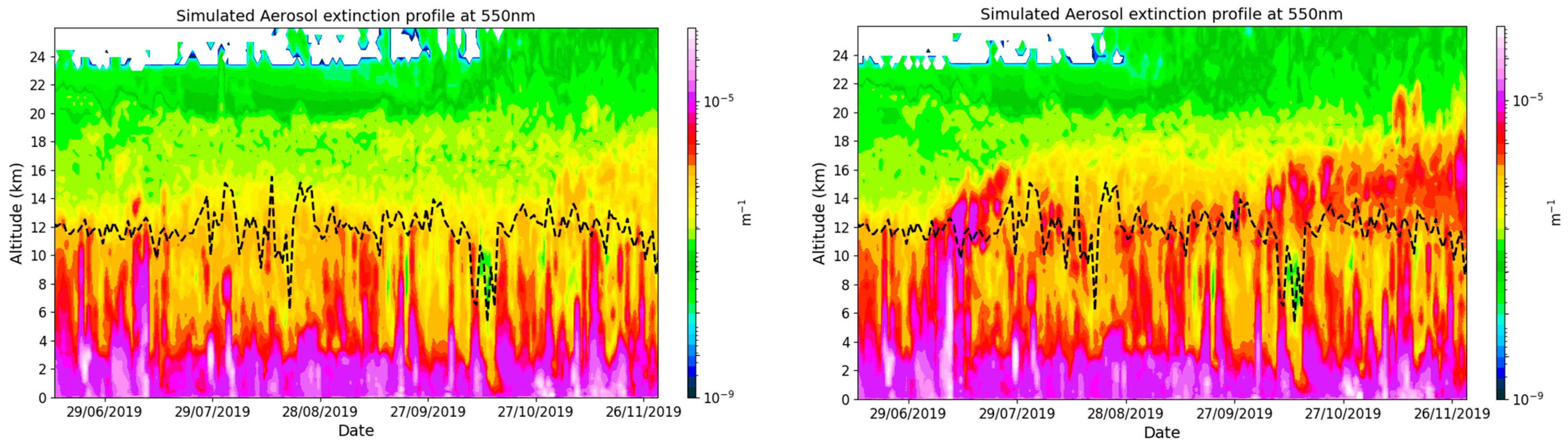
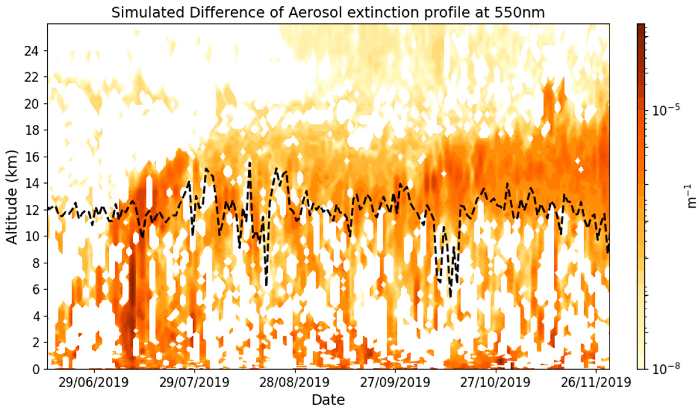
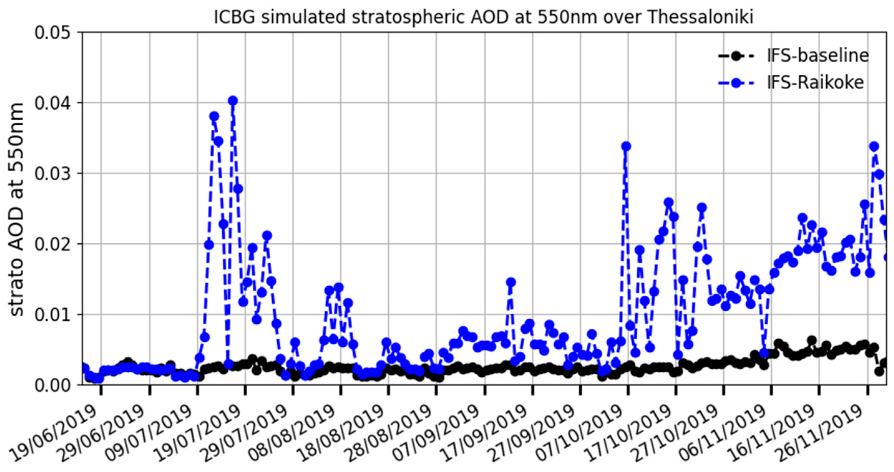
3.3. Identification of the Stratospheric Layer Origin Using CAMS ICBG Simulations
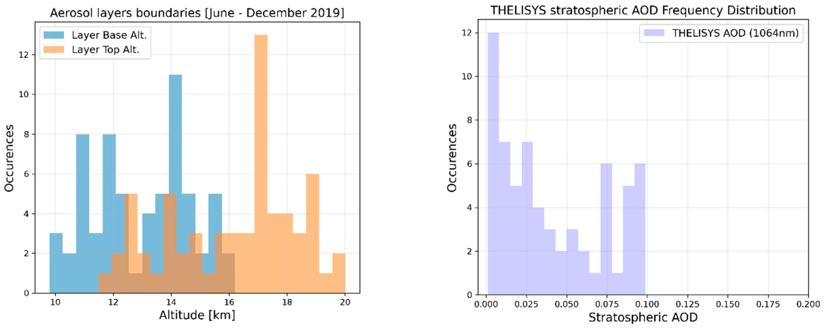
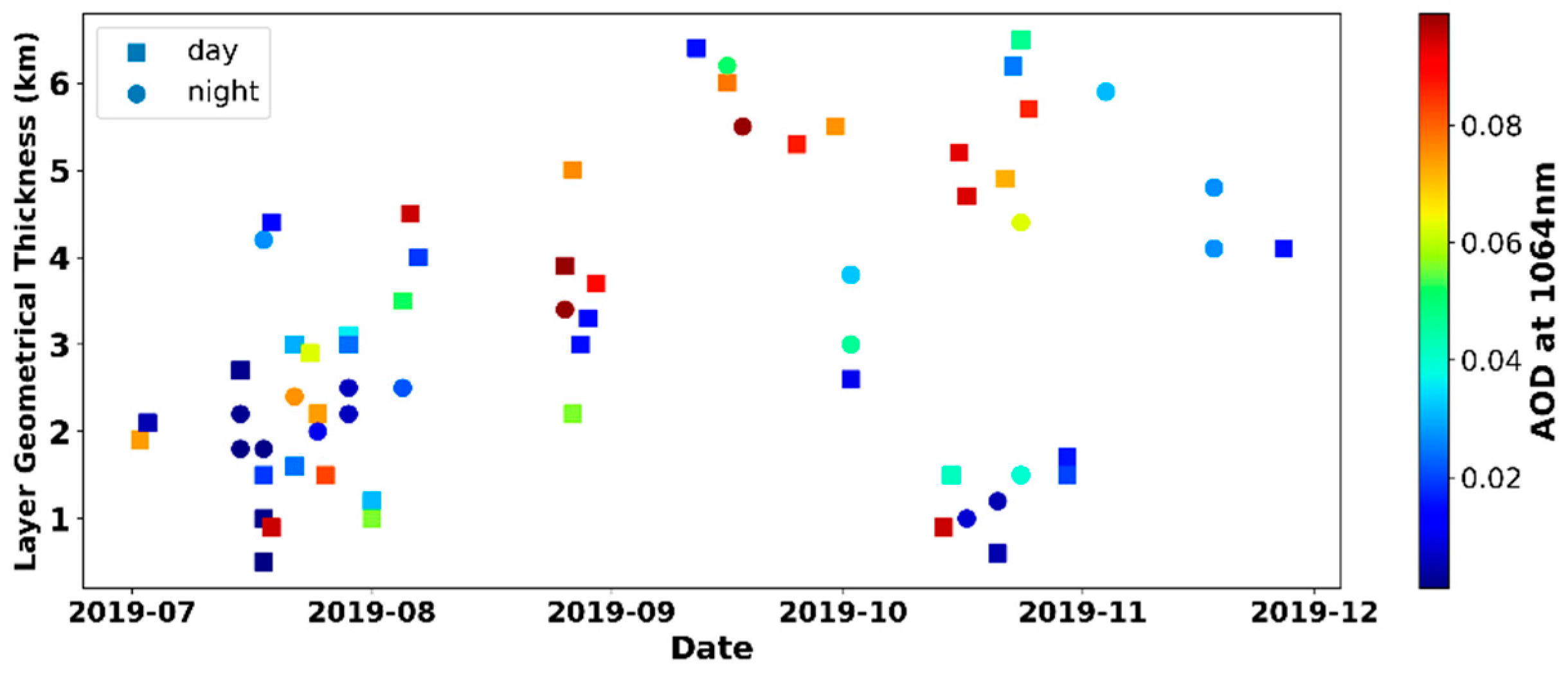
3.4. Geometrical and Optical Aerosol Properties from Ground- and Space-Based Measurements
3.5. Correlative Stratospheric Measurements for 25 July 2019
4. Conclusions
- i.
- Complex stratospheric aerosol conditions with simultaneously occurring volcanic and smoke layers took place in the second half of 2019 over Thessaloniki, Greece. A persistent stratospheric layer with variable geometric boundaries (from 10 up to 20 km) was monitored with a Raman lidar over Thessaloniki, Greece, starting from July 2019, stimulating the investigation of the main source of this persistent, but not stable, aerosol layer. We further probed the lower stratosphere for this aerosol layer during the period July–December 2019 using space-borne CALIOP/CALIPSO and OMPS-LP observations. A CAMS data assimilation experiment of the Raikoke eruption also confirmed that the SO2 plume arrived over the Mediterranean and Thessaloniki station, corroborated by CALIPSO measurements which indicated that the main composition of the layer was sulphate particles. This was until August, when local or high northern latitudes (i.e., Alaska, Alberta, Siberia) fires also contaminated the lower stratosphere. All sensors with different detection limitations captured the temporal and height variability of the observed layer above Thessaloniki during the complex stratospheric aerosol conditions of 2019. In short, the ground-based system monitored the stratospheric layer with high temporal sampling and high vertical resolution, denoting an increased thickness till the end of 2019, whilst the correlative CALIPSO and OMPS-LP retrievals, having different temporal coverage, enhanced the spatial sampling by capturing the stratospheric features after the eruption. On top of that, the model simulations suggested the presence of volcanic particles in the stratosphere and the CALIPSO typing scheme identified the plume’s origin and geometrical and optical properties. The combined results of ground measurements, space observations, and model simulations are summarized as follows. The pronounced aerosol layer was present from July 2019 to the end of that year. During July, volcanic sulphate aerosol layers (particle linear depolarization ratio < 0.08) with a 1–3 km vertical extent were mainly identified in the stratosphere over Thessaloniki, while after August, the plume heights showed significant month-to-month variability and a broadening (with thickness greater than 3 km) towards lower altitudes.
- ii.
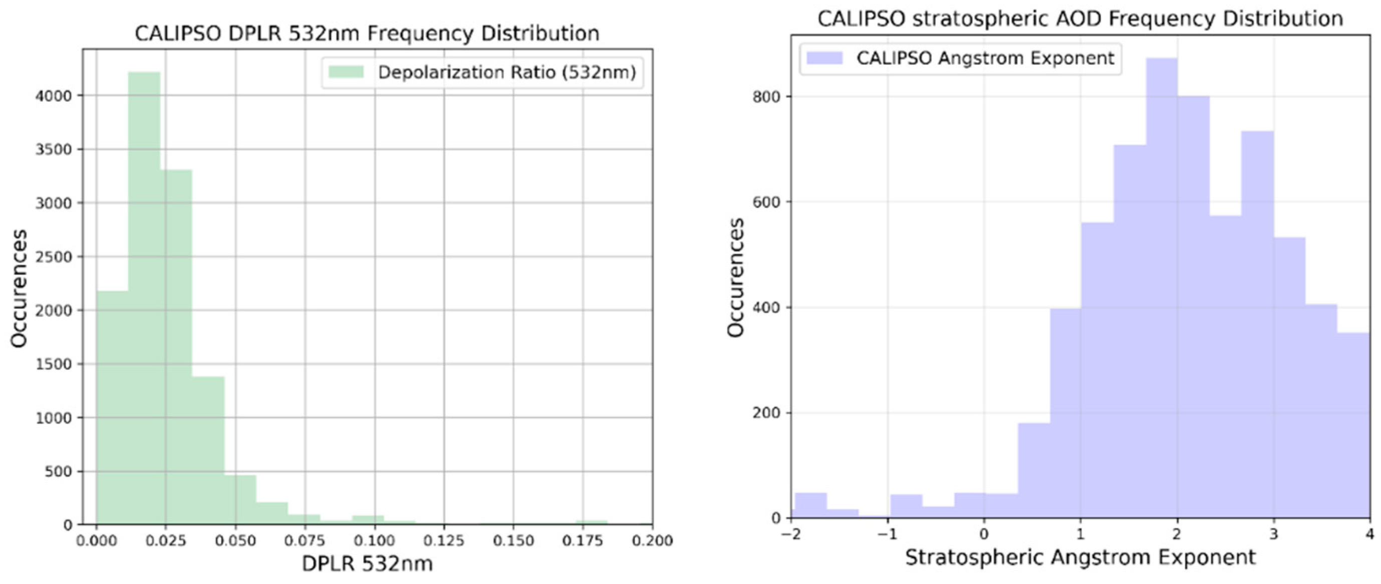
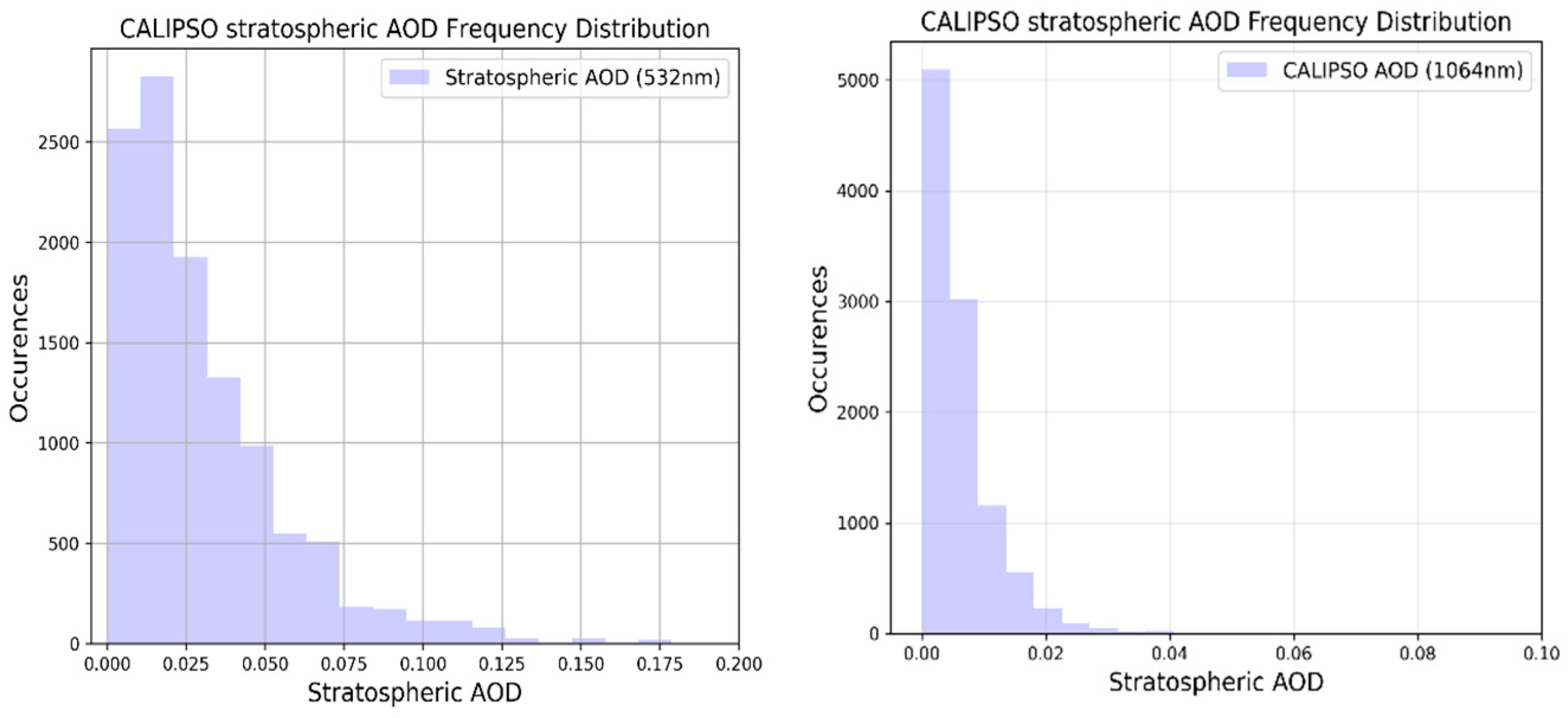
- The aerosol optical thickness was found to be in the range between 0.004 and 0.125 (visible) and 0.001 and 0.095 (infrared) and the particle depolarization of the detected stratospheric plume was found to be 0.03 ± 0.04, indicative of spherical particles such as sulphate aerosols.
- iii.
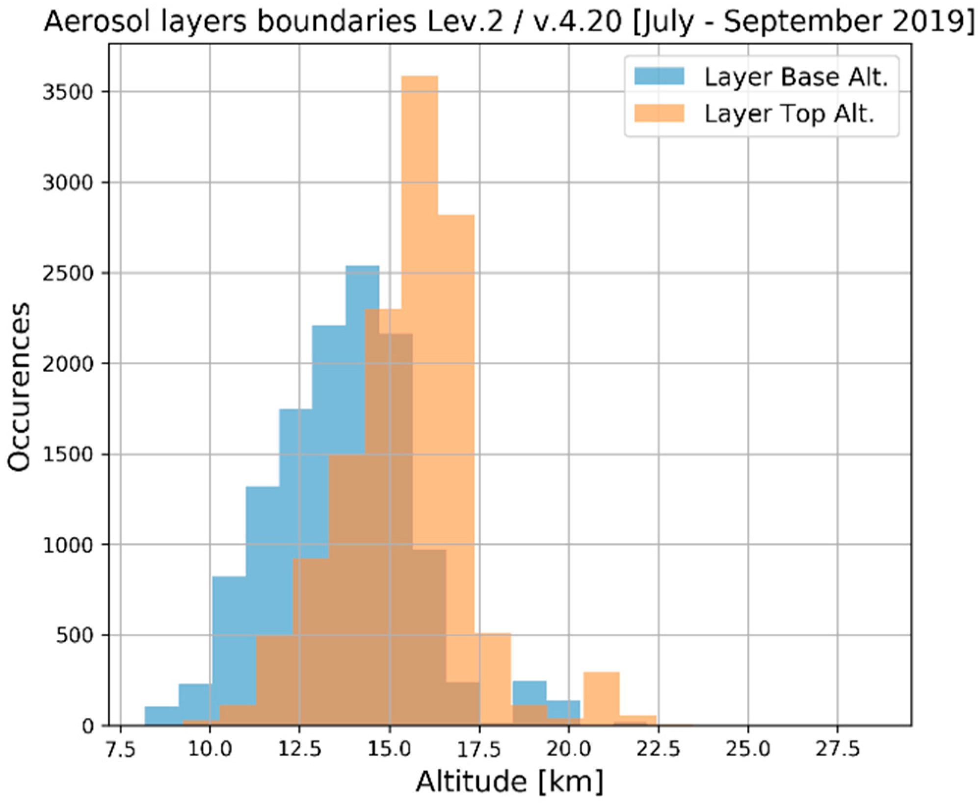
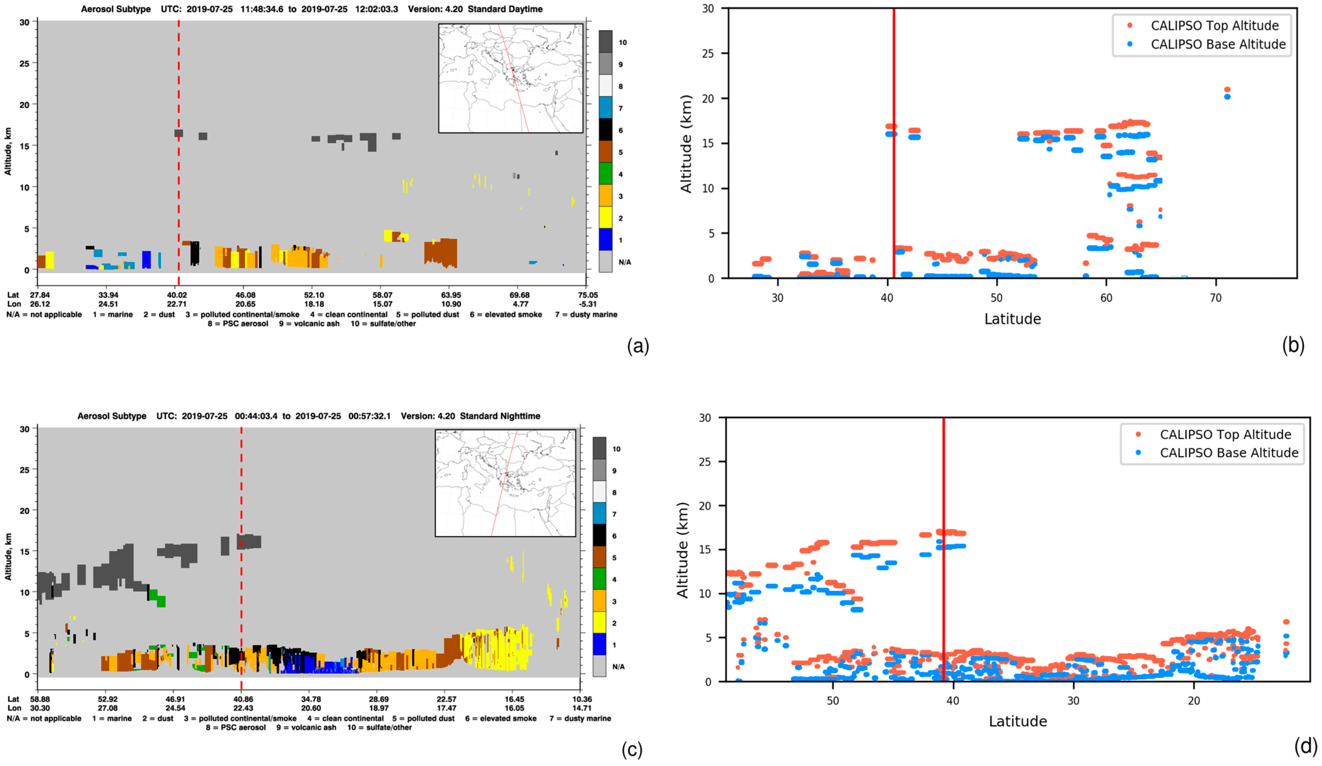
- The CALIPSO aerosol-typing identified the volcanic sulphate aerosol type as the dominant type of the stratospheric plume for ~91% of the identified stratospheric layers throughout the year of 2019, whilst a small number of aerosol layers (~9%) were classified as smoke and ash particles, possibly originating from Siberian and Canadian fires. The smoke particles were nearly always located below the identified sulphate particles, while the more pronounced smoke layers were identified beyond and to the North of Thessaloniki.
- iv.
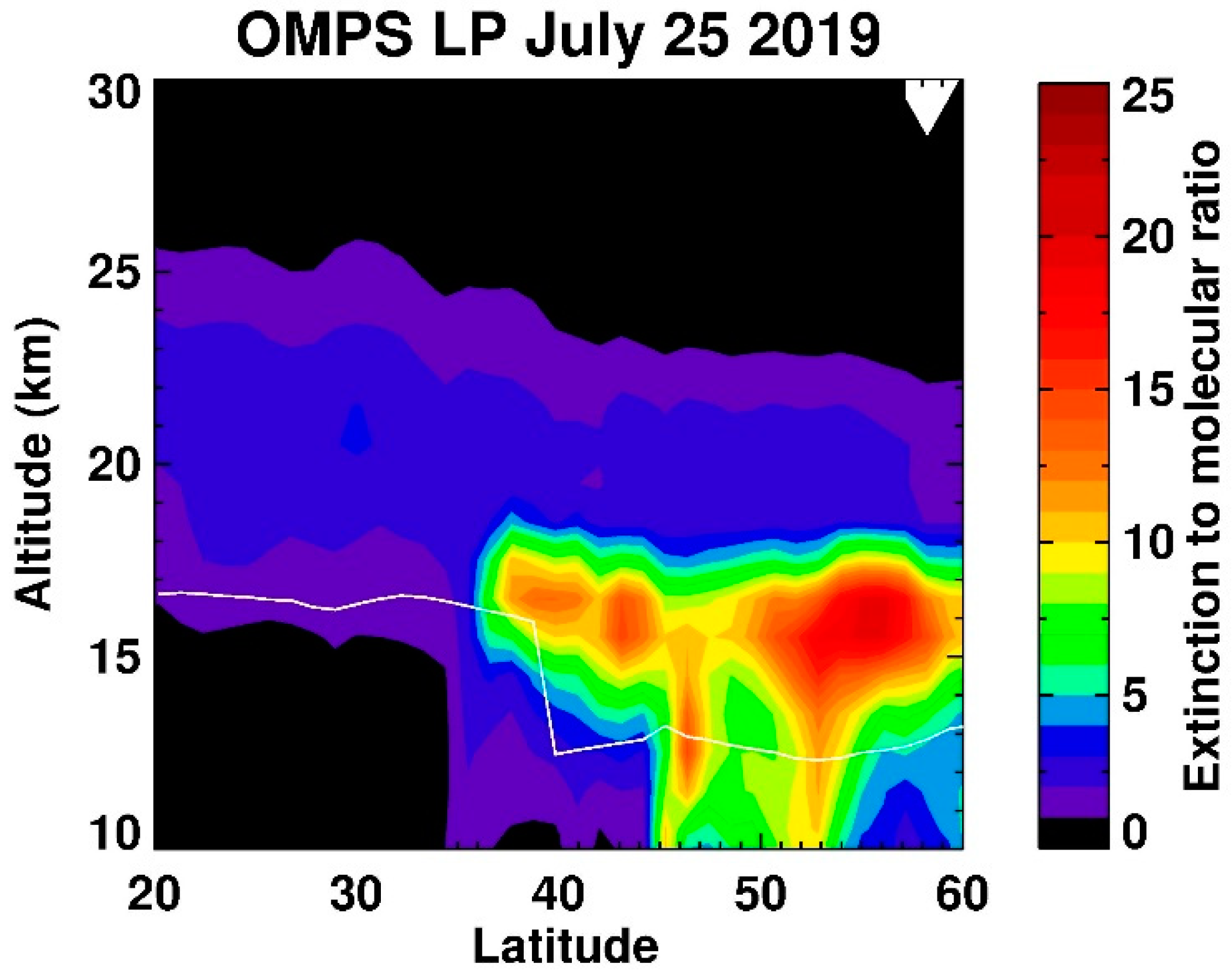
- The consistency of the active and passive measurements and CAMS assimilations was identified for the case study of the 25 July. The case presented, in detail, the geometrical boundaries (~16 km) and the optical signature of the stratospheric plume from the different sources and the CALIPSO aerosol-typing identified the volcanic sulphate aerosol type as the predominant type of the stratospheric plume.
Supplementary Materials
Author Contributions
Funding
 .
.Data Availability Statement
Acknowledgments
Conflicts of Interest
References
- Thompson, D.W.; Solomon, S. Understanding recent stratospheric climate change. J. Clim. 2009, 22, 1934–1943. [Google Scholar] [CrossRef]
- Domeisen, D.I.V.; Butler, A.H. Stratospheric drivers of extreme events at the Earth’s surface. Commun. Earth Env. 2020, 1, 59. [Google Scholar] [CrossRef]
- Rasch, P.J.; Tilmes, S.; Turco, R.P.; Robock, A.; Oman, L.; Chen, C.-C.; Stenchikov, G.L.; Garcia, R.R. An overview of geoengineering of climate using stratospheric sulphate aerosols. Philos. Trans. R. Soc. A 2008, 366, 4007–4037. [Google Scholar] [CrossRef] [PubMed]
- Hofmann, D.; Barnes, J.; O’Neill, M.; Trudeau, M.; Neely, R. Increase in background stratospheric aerosol observed with lidar at Mauna Loa Observatory and Boulder, Colorado. Geophys. Res. Lett. 2009, 36, L15808. [Google Scholar] [CrossRef]
- Vernier, J.-P.; Fairlie, T.D.; Deshler, T.; Natarajan, M.; Knepp, T.; Foster, K.; Wienhold, F.G.; Bedka, K.M.; Thomason, L.; Trepte, C. In situ and space-based observations of the Kelud volcanic plume: The persistence of ash in the lower stratosphere. J. Geophys. Res. Atmos. 2016, 121, 11104–11118. [Google Scholar] [CrossRef] [PubMed]
- Kremser, S.; Thomason, L.W.; von Hobe, M.; Hermann, M.; Deshler, T.; Timmreck, C.; Toohey, M.; Stenke, A.; Schwarz, J.P.; Weigel, R.; et al. Stratospheric aerosol—Observations, processes, and impact on climate. Rev. Geophys. 2016, 54, 278–335. [Google Scholar] [CrossRef]
- Fromm, M.; Lindsey, D.T.; Servranckx, R.; Yue, G.; Trickl, T.; Sica, R.; Doucet, P.; Godin-Beekmann, S. The untold story of pyrocumulonimbus. Bull. Am. Meteorol. Soc. 2010, 91, 1193–1209. [Google Scholar] [CrossRef]
- Peterson, D.A.; Campbell, J.R.; Hyer, E.J.; Fromm, M.D.; Kablick, G.P.; Cossuth, J.H.; DeLand, M.T. Wildfire-driven thunderstorms cause a volcano-like stratospheric injection of smoke. NPJ Clim. Atmos. Sci. 2018, 2018, 30. [Google Scholar] [CrossRef]
- Yu, P.; Toon, O.B.; Bardeen, C.G.; Zhu, Y.; Rosenlof, K.H.; Portmann, R.W.; Thornberry, T.D.; Gao, R.; Davis, S.M.; Wolf, E.T.; et al. Black carbon lofts wildfire smoke high into the stratosphere to form a persistent plume. Science 2019, 365, 587–590. [Google Scholar] [CrossRef]
- Torres, O.; Bhartia, P.K.; Taha, G.; Jethva, H.; Das, S.; Colarco, P.; Krotkov, N.; Omar, A.; Ahn, C. Stratospheric Injection of Massive Smoke Plume from Canadian Boreal Fires in 2017 as seen by DSCOVR-EPIC, CALIOP and OMPS-LP Observations. J. Geophys. Res.-Atmos. Atmos. 2020, 125, e2020JD032579. [Google Scholar] [CrossRef]
- Mattis, I.; Siefert, P.; Müller, D.; Tesche, M.; Hiebsch, A.; Kanitz, T.; Schmidt, J.; Finger, F.; Wandinger, U.; Ansmann, A. Volcanic aerosol layers observed with multiwavelength Raman lidar over central Europe in 2008–2009. J. Geophys. Res.-Atmos. 2010, 115, D00L04. [Google Scholar] [CrossRef]
- Pappalardo, G.; Wandinger, U.; Mona, L.; Hiebsch, A.; Mattis, I.; Amodeo, A.; Ansmann, A.; Seifert, P.; Linné, H.; Apituley, A.; et al. EARLINET correlative measurements for CALIPSO: First intercomparison results. J. Geophys. Res. 2010, 115, D00H19. [Google Scholar] [CrossRef]
- Sicard, M.; Guerrero-Rascado, J.L.; Navas-Guzmán, F.; Preißler, J.; Molero, F.; Tomás, S.; Bravo-Aranda, J.A.; Comerón, A.; Rocadenbosch, F.; Wagner, F.; et al. Monitoring of the Eyjafjallajökull volcanic aerosol plume over the Iberian Peninsula by means of four EARLINET lidar stations. Atmos. Chem. Phys. 2012, 12, 3115–3130. [Google Scholar] [CrossRef]
- Trickl, T.; Giehl, H.; Jäger, H.; Vogelmann, H. 35 yr of stratospheric aerosol measurements at Garmisch-Partenkirchen: From Fuego to Eyjafjallajökull, and beyond. Atmos. Chem. Phys. 2013, 13, 5205–5225. [Google Scholar] [CrossRef]
- Khaykin, S.M.; Godin-Beekmann, S.; Keckhut, P.; Hauchecorne, A.; Jumelet, J.; Vernier, J.-P.; Bourassa, A.; Degenstein, D.A.; Rieger, L.A.; Bingen, C.; et al. Variability and evolution of the midlatitude stratospheric aerosol budget from 22 years of ground-based lidar and satellite observations. Atmos. Chem. Phys. 2017, 17, 1829–1845. [Google Scholar] [CrossRef]
- Boselli, A.; Scollo, S.; Leto, G.; Sanchez, R.Z.; Sannino, A.; Wang, X.; Coltelli, M.; Spinelli, N. First volcanic plume measurements by an elastic/raman lidar close to the Etna summit craters. Front. Earth Sci. 2018, 6, 125. [Google Scholar] [CrossRef]
- Zuev, V.V.; Burlakov, V.D.; Nevzorov, A.V.; Pravdin, V.L.; Savelieva, E.S.; Gerasimov, V.V. 30-year lidar observations of the stratospheric aerosol layer state over Tomsk (Western Siberia, Russia). Atmos. Chem. Phys. 2017, 17, 3067–3081. [Google Scholar] [CrossRef]
- Ansmann, A.; Tesche, M.; Seifert, P.; Groß, S.; Freudenthaler, V.; Apituley, A.; Wilson, K.M.; Serikov, I.; Linné, H.; Heinold, B.; et al. Ash and fine-mode particle mass profiles from EARLINET-AERONET observations over central Europe after the eruptions of the Eyjafjallajökull volcano in 2010. J. Geophys. Res.-Atmos. 2011, 116, D00U02. [Google Scholar] [CrossRef]
- Deshler, T.; Hervig, M.; Hofmann, D.; Rosen, J.; Liley, J. Thirty years of in situ stratospheric aerosol size distribution measurements from Laramie, Wyoming (41N), using balloon-borne instruments. J. Geophys. Res.-Atmos. 2003, 108, 4167. [Google Scholar] [CrossRef]
- Vernier, J.P.; Pommereau, J.P.; Garnier, A.; Pelon, J.; Larsen, N.; Nielsen, J.; Christensen, T.; Cairo, F.; Thomason, L.W.; Leblanc, T.; et al. Tropical stratospheric aerosol layer from CALIPSO lidar observations. J. Geophys. Res.-Atmos. 2009, 114, D4. [Google Scholar] [CrossRef]
- Toledano, C.; Bennouna, Y.; Cachorro, V.; Ortiz de Galisteo, J.P.; Stohl, A.; Stebel, K.; Kristiansen, N.I.; Olmo, F.J.; Lyamani, H.; Obregón, M.A.; et al. Aerosol properties of the Eyjafjallajökull ash derived from sun photometer and satellite observations over the Iberian Peninsula. Atmos. Environ. 2012, 48, 22–32. [Google Scholar] [CrossRef]
- Chouza, F.; Leblanc, T.; Barnes, J.; Brewer, M.; Wang, P.; Koon, D. Long-term (1999–2019) variability of stratospheric aerosol over Mauna Loa, Hawaii, as seen by two co-located lidars and satellite measurements. Atmos. Chem. Phys. 2020, 20, 6821–6839. [Google Scholar] [CrossRef]
- McCormick, M.; Veiga, R. SAGE II measurements of early Pinatubo aerosols. Geophys. Res. Lett. 1992, 19, 155–158. [Google Scholar] [CrossRef]
- Vaughan, G.; Wareing, D.; Ricketts, H. Measurement Report: Lidar Measurements of Stratospheric Aerosol Following the 2019 Raikoke and Ulawun Volcanic Eruptions. Atmos. Chem. Phys. 2021, 21, 5597–5604. [Google Scholar] [CrossRef]
- de Leeuw, J.; Schmidt, A.; Witham, C.S.; Theys, N.; Taylor, I.A.; Grainger, R.G.; Pope, R.J.; Haywood, J.; Osborne, M.; Kristiansen, N.I. The 2019 Raikoke volcanic eruption—Part 1: Dispersion model simulations and satellite retrievals of volcanic sulfur dioxide. Atmos. Chem. Phys. 2021, 21, 10851–10879. [Google Scholar] [CrossRef]
- Muser, L.O.; Hoshyaripour, G.A.; Bruckert, J.; Horváth, Á.; Malinina, E.; Wallis, S.; Prata, F.J.; Rozanov, A.; von Savigny, C.; Vogel, H.; et al. Particle aging and aerosol–radiation interaction affect volcanic plume dispersion: Evidence from the Raikoke 2019 eruption. Atmos. Chem. Phys. 2020, 20, 15015–15036. [Google Scholar] [CrossRef]
- Grebennikov, V.S.; Zubachev, D.S.; Korshunov, V.A.; Sakhibgareev, D.G.; Chernikh, I.A. Observations of Stratospheric Aerosol at Rosgidromet Lidar Stations after the Eruption of the Raikoke Volcano in June 2019. Atmos. Ocean. Opt. 2020, 33, 519–523. [Google Scholar] [CrossRef]
- Khaykin, S.M.; de Laat, A.T.J.; Godin-Beekmann, S.; Hauchecorne, A.; Ratynski, M. Unexpected self-lofting and dynamical confinement of volcanic plumes: The Raikoke 2019 case. Sci. Rep. 2022, 12, 22409. [Google Scholar] [CrossRef]
- Ohneiser, K.; Ansmann, A.; Chudnovsky, A.; Engelmann, R.; Ritter, C.; Veselovskii, I.; Baars, H.; Gebauer, H.; Griesche, H.; Radenz, M.; et al. The unexpected smoke layer in the High Arctic winter stratosphere during MOSAiC 2019–2020. Atmos. Chem. Phys. 2021, 21, 15783–15808. [Google Scholar] [CrossRef]
- Junghenn Noyes, K.T.; Kahn, R.A.; Limbacher, J.A.; Li, Z. Canadian and Alaskan wildfire smoke particle properties, their evolution, and controlling factors, from satellite observations. Atmos. Chem. Phys. 2022, 22, 10267–10290. [Google Scholar] [CrossRef]
- Pappalardo, G.; Amodeo, A.; Apituley, A.; Comeron, A.; Freudenthaler, V.; Linné, H.; Ansmann, A.; Bösenberg, J.; D’Amico, G.; Mattis, I.; et al. EARLINET: Towards an advanced sustainable European aerosol lidar network. Atmos. Meas. Tech. 2014, 7, 2389–2409. [Google Scholar] [CrossRef]
- Siomos, N.; Balis, D.S.; Voudouri, K.A.; Giannakaki, E.; Filioglou, M.; Amiridis, V.; Papayannis, A.; Fragkos, K. Are EARLINET and AERONET climatologies consistent? The case of Thessaloniki, Greece. Atmos. Chem. Phys. 2018, 18, 11885–11903. [Google Scholar] [CrossRef]
- Voudouri, K.A.; Siomos, N.; Michailidis, K.; D’Amico, G.; Mattis, I.; Balis, D. Consistency of the Single Calculus Chain Optical Products with Archived Measurements from an EARLINET Lidar Station. Remote Sens. 2020, 12, 3969. [Google Scholar] [CrossRef]
- Platt, C.M.R.; Young, S.A.; Carswell, A.I.; Pal, S.R.; McCormick, M.P.; Winker, D.M.; DelGuasta, M.; Stefanutti, L.; Eberhard, W.L.; Hardesty, M.; et al. The experimental cloud lidar pilot study (ECLIPS) for cloud-radiation research. Bull. Am. Meteorol. Soc. 1994, 75, 1635–1654. [Google Scholar] [CrossRef]
- Klett, J.D. Lidar inversion with variable backscatter to extinction ratios. Appl. Opt. 1985, 24, 1638–1643. [Google Scholar] [CrossRef]
- Ansmann, A.; Riebesell, M.; Weitkamp, C. Measurement of atmospheric aerosol extinction profiles with a Raman lidar. Opt. Lett. 1990, 15, 746–748. [Google Scholar] [CrossRef]
- Chen, W.N.; Chiang, C.W.; Nee, J.B. Lidar ratio and depolarization ratio for cirrus clouds. Appl. Opt. 2002, 41, 6470–6476. [Google Scholar] [CrossRef]
- Voudouri, K.A.; Giannakaki, E.; Komppula, M.; Balis, D. Variability in cirrus cloud properties using a PollyXT Raman lidar over high and tropical latitudes. Atmos. Chem. Phys. 2020, 20, 4427–4444. [Google Scholar] [CrossRef]
- Giannakaki, E.; Balis, D.S.; Amiridis, V.; Kazadzis, S. Optical and geometrical characteristics of cirrus clouds over a Southern European lidar station. Atmos. Chem. Phys. 2007, 7, 5519–5530. [Google Scholar] [CrossRef]
- Winker, D.M.; Vaughan, M.A.; Omar, A.; Hu, Y.; Powell, K.A.; Liu, Z.; Hunt, W.H.; Young, S.A. Overview of the CALIPSO Mission and CALIOP Data Processing Algorithms. J. Atmos. Ocean. Technol. 2009, 26, 2310–2323. Available online: https://journals.ametsoc.org/view/journals/atot/26/11/2009jtecha1281_1.xml (accessed on 15 November 2023). [CrossRef]
- Kim, M.-H.; Omar, A.H.; Tackett, J.L.; Vaughan, M.A.; Winker, D.M.; Trepte, C.R.; Hu, Y.; Liu, Z.; Poole, L.R.; Pitts, M.C.; et al. The CALIPSO version 4 automated aerosol classification and lidar ratio selection algorithm. Atmos. Meas. Tech. 2018, 11, 6107–6135. [Google Scholar] [CrossRef]
- Vaughan, M.A.; Powell, K.A.; Winker, D.M.; Hostetler, C.A.; Kuehn, R.E.; Hunt, W.H.; Getzewich, B.J.; Young, S.A.; Liu, Z.; McGill, M.J. Fully Automated Detection of Cloud and Aerosol Layers in the CALIPSO Lidar Measurements. J. Atmos. Ocean. Tech. 2009, 26, 2034–2050. [Google Scholar] [CrossRef]
- Liu, Z.; Kar, J.; Zeng, S.; Tackett, J.; Vaughan, M.; Avery, M.; Pelon, J.; Getzewich, B.; Lee, K.-P.; Magill, B.; et al. Discriminating between Clouds and Aerosols in the Caliop Version 4.1 Data Products. Atmos. Meas. Tech. 2019, 12, 703–734. [Google Scholar] [CrossRef]
- Tackett, J.L.; Kar, J.; Vaughan, M.A.; Getzewich, B.J.; Kim, M.-H.; Vernier, J.-P.; Omar, A.H.; Magill, B.E.; Pitts, M.C.; Winker, D.M. The CALIPSO version 4.5 stratospheric aerosol subtyping algorithm. Atmos. Meas. Tech. 2023, 16, 745–768. [Google Scholar] [CrossRef]
- Taha, G. OMPS-NPP L2 LP Aerosol Extinction Vertical Profile Swath Daily 3slit V2, Greenbelt, MD, USA, Goddard Earth Sciences Data and Information Services Center (GES DISC). 2020. Available online: https://disc.gsfc.nasa.gov/datasets/OMPS_NPP_LP_L2_AER_DAILY_2/summary (accessed on 2 May 2023).
- Chen, Z.; Bhartia, P.K.; Loughman, R.; Colarco, P.; DeLand, M. Improvement of stratospheric aerosol extinction retrieval from OMPS/LP using a new aerosol model. Atmos. Meas. Tech. 2018, 11, 6495–6509. [Google Scholar] [CrossRef] [PubMed]
- Taha, G.; Loughman, R.; Colarco, P.R.; Zhu, T.; Thomason, L.W.; Jaross, G. Tracking the 2022 Hunga Tonga-Hunga Ha’apai aerosol cloud in the upper and middle stratosphere using space-based observations. Geophys. Res. Lett. 2022, 49, e2022GL100091. [Google Scholar] [CrossRef] [PubMed]
- Taha, G.; Loughman, R.; Zhu, T.; Thomason, L.; Kar, J.; Rieger, L.; Bourassa, A. OMPS LP Version 2.0 multi-wavelength aerosol extinction coefficient retrieval algorithm. Atmos. Meas. Tech. 2021, 14, 1015–1036. [Google Scholar] [CrossRef]
- Kloss, C.; Berthet, G.; Sellitto, P.; Ploeger, F.; Taha, G.; Tidiga, M.; Eremenko, M.; Bossolasco, A.; Jégou, F.; Renard, J.-B.; et al. Stratospheric aerosol layer perturbation caused by the 2019 Raikoke and Ulawun eruptions and their radiative forcing. Atmos. Chem. Phys. 2021, 21, 535–560. [Google Scholar] [CrossRef]
- Gorkavyi, N.; Krotkov, N.; Li, C.; Lait, L.; Colarco, P.; Carn, S.; DeLand, M.; Newman, P.; Schoeberl, M.; Taha, G.; et al. Tracking aerosols and SO2 clouds from the Raikoke eruption: 3D view from satellite observations. Atmos. Meas. Tech. 2021, 14, 7545–7563. [Google Scholar] [CrossRef]
- Wells, A.F.; Jones, A.; Osborne, M.; Damany-Pearce, L.; Partridge, D.G.; Haywood, J.M. Including ash in UKESM1 model simulations of the Raikoke volcanic eruption reveals improved agreement with observations. Atmos. Chem. Phys. 2023, 23, 3985–4007. [Google Scholar] [CrossRef]
- Peuch, V.; Engelen, R.; Rixen, M.; Dee, D.; Flemming, J.; Suttie, M.; Ades, M.; Agustí-Panareda, A.; Ananasso, C.; Andersson, E.; et al. The Copernicus Atmosphere Monitoring Service: From research to operations. Bull. Am. Meteorol. Soc. 2022, 103, E2650–E2668. [Google Scholar] [CrossRef]
- Inness, A.; Ades, M.; Balis, D.; Efremenko, D.; Flemming, J.; Hedelt, P.; Koukouli, M.-E.; Loyola, D.; Ribas, R. Evaluating the assimilation of S5P/TROPOMI near real-time SO2 columns and layer height data into the CAMS integrated forecasting system (CY47R1), based on a case study of the 2019 Raikoke eruption. Geosci. Model Dev. 2022, 15, 971–994. [Google Scholar] [CrossRef]
- Hedelt, P.; Efremenko, D.S.; Loyola, D.G.; Spurr, R.; Clarisse, L. Sulfur dioxide layer height retrieval from Sentinel-5 Precursor/TROPOMI using FP_ILM. Atmos. Meas. Tech. 2019, 12, 5503–5517. [Google Scholar] [CrossRef]
- Koukouli, M.-E.; Michailidis, K.; Hedelt, P.; Taylor, I.A.; Inness, A.; Clarisse, L.; Balis, D.; Efremenko, D.; Loyola, D.; Grainger, R.G.; et al. Volcanic SO2 layer height by TROPOMI/S5P: Evaluation against IASI/MetOp and CALIOP/CALIPSO observations. Atmos. Chem. Phys. 2022, 22, 5665–5683. [Google Scholar] [CrossRef]
- Yarwood, G.; Rao, S.; Yocke, M.; Whitten, G.Z. Updates to the Carbon Bond Mechanism: CB05. Final Report to the US Environmental Protection Agency; RT-0400675; Yocke and Company: Novato, CA, USA, 2005. [Google Scholar]
- Huijnen, V.; Williams, J.; van Weele, M.; van Noije, T.; Krol, M.; Dentener, F.; Segers, A.; Houweling, S.; Peters, W.; de Laat, J.; et al. The global chemistry transport model TM5: Description and evaluation of the tropospheric chemistry version 3.0. Geosci. Model Dev. 2010, 3, 445–473. [Google Scholar] [CrossRef]
- Mann, G.W.; Carslaw, K.S.; Spracklen, D.V.; Ridley, D.A.; Manktelow, P.T.; Chipperfield, M.P.; Pickering, S.J.; Johnson, C.E. Description and evaluation of GLOMAP-mode: A modal global aerosol microphysics model for the UKCA composition-climate model. Geosci. Model Dev. 2010, 3, 519–551. [Google Scholar] [CrossRef]
- Huijnen, V.; Flemming, J.; Chabrillat, S.; Errera, Q.; Christophe, Y.; Blechschmidt, A.-M.; Richter, A.; Eskes, H. C-IFS-CB05-BASCOE: Stratospheric chemistry in the Integrated Forecasting System of ECMWF. Geosci. Model Dev. 2016, 9, 3071–3091. [Google Scholar] [CrossRef]
- Cameron, W.; Bernath, D.P.; Boone, C. Sulfur dioxide from the atmospheric chemistry experiment (ACE) satellite. J. Quant. Spectrosc. Radiat. Transf. 2021, 258, 107341. [Google Scholar] [CrossRef]
- Ansmann, A.; Ohneiser, K.; Chudnovsky, A.; Baars, H.; Engelmann, R. CALIPSO Aerosol-Typing Scheme Misclassified Stratospheric Fire Smoke: Case Study From the 2019 Siberian Wildfire Season. Front. Environ. Sci. 2021, 9, 769852. [Google Scholar] [CrossRef]
- Hoffmann, L.; Spang, R. An assessment of tropopause characteristics of the ERA5 and ERA-Interim meteorological reanalyses. Atmos. Chem. Phys. 2022, 22, 4019–4046. [Google Scholar] [CrossRef]
- Michailidis, K.; Siomos, N.; Balis, D. Performance of the Aerosol Species Separation Algorithm (ASSA) Using Data from a Raman-Depolarization Lidar System at Thessaloniki, Greece. Environ. Sci. Proc. 2023, 26, 70. [Google Scholar] [CrossRef]


| Spatial Resolution | Temporal Coverage | |
|---|---|---|
| THELISYS | 7.5 m (1064 nm) | Monday and Thursday following the EARLINET schedule [31] |
| CALIPSO | Horizontal: 1000 m|Vertical: 60 m | 16-day repeat cycle |
| OMPS-LP | Horizontal: ~250 km|Vertical: 1.6–1.8 km | 16-day repeat cycle |
| CAMS LHexp | Horizontal: 40 km|Vertical: 137 model levels between the surface and 0.01 hPa | 6-hourly from 22 June to 29 September 2019 |
| ICBG | Horizontal: 80 km|Vertical: 137 model levels between the surface and 0.01 hPa | 3-hourly from 1 June to 30 November 2019 |
| Geophysical Parameter | Aim in This Paper | |
|---|---|---|
| THELISYS | Layer top and base altitude Backscatter extinction profiles at 532 and 1064 nm Stratospheric AOD at 1064 nm | Layer temporal evolution, geometrical boundaries, AOD at 1064 nm |
| CALIPSO | Layer top and base altitude Stratospheric AOD at 532 nm and 1064 nm Particle depolarization ratio at 532 nm Aerosol classification | Geometrical boundaries, AOD at 532 nm, aerosol typing |
| OMPS-LP | Extinction profile at 997 nm Stratospheric AOD at 997 nm | Layer temporal evolution, AOD at 997 nm |
| CAMS LHexp | SO2 plume [D.U.] | SO2 transport around the NH |
| ICBG | Stratospheric AOD at 550 nm Extinction profile at 550 nm | Layer temporal and spatial evolution, AOD at 550 nm |
| THELISYS | CALIPSO | ICBG | OMPS-LP | ||
|---|---|---|---|---|---|
| Daytime | Night-Time | ||||
| Layer Base Height (km) | 16.2 | 16.04 | 15.40 ± 1.71 | 14.77 | 14.47 ± 0.53 |
| Layer Top Height (km) | 16.8 | 16.44 | 16.68 ± 1.32 | 16.13 | 17.88 ± 0.13 |
| PLDR | <0.05 | 0.086 | 0.018 ± 0.003 | n/a | n/a |
| AOD IR (wavelength in nm) | 0.0095 (1064) | n/a | 0.002 ± 0.006 | n/a | 0.007 ± 0.0015 (997) |
| AOD VIS (wavelength in nm) | 0.012 (532) | 0.017 (532) | 0.023 ± 0.03(532) | 0.009 (550) | n/a |
Disclaimer/Publisher’s Note: The statements, opinions and data contained in all publications are solely those of the individual author(s) and contributor(s) and not of MDPI and/or the editor(s). MDPI and/or the editor(s) disclaim responsibility for any injury to people or property resulting from any ideas, methods, instructions or products referred to in the content. |
© 2023 by the authors. Licensee MDPI, Basel, Switzerland. This article is an open access article distributed under the terms and conditions of the Creative Commons Attribution (CC BY) license (https://creativecommons.org/licenses/by/4.0/).
Share and Cite
Voudouri, K.A.; Michailidis, K.; Koukouli, M.-E.; Rémy, S.; Inness, A.; Taha, G.; Peletidou, G.; Siomos, N.; Balis, D.; Parrington, M. Investigating a Persistent Stratospheric Aerosol Layer Observed over Southern Europe during 2019. Remote Sens. 2023, 15, 5394. https://doi.org/10.3390/rs15225394
Voudouri KA, Michailidis K, Koukouli M-E, Rémy S, Inness A, Taha G, Peletidou G, Siomos N, Balis D, Parrington M. Investigating a Persistent Stratospheric Aerosol Layer Observed over Southern Europe during 2019. Remote Sensing. 2023; 15(22):5394. https://doi.org/10.3390/rs15225394
Chicago/Turabian StyleVoudouri, Kalliopi Artemis, Konstantinos Michailidis, Maria-Elissavet Koukouli, Samuel Rémy, Antje Inness, Ghassan Taha, Georgia Peletidou, Nikolaos Siomos, Dimitrios Balis, and Mark Parrington. 2023. "Investigating a Persistent Stratospheric Aerosol Layer Observed over Southern Europe during 2019" Remote Sensing 15, no. 22: 5394. https://doi.org/10.3390/rs15225394
APA StyleVoudouri, K. A., Michailidis, K., Koukouli, M.-E., Rémy, S., Inness, A., Taha, G., Peletidou, G., Siomos, N., Balis, D., & Parrington, M. (2023). Investigating a Persistent Stratospheric Aerosol Layer Observed over Southern Europe during 2019. Remote Sensing, 15(22), 5394. https://doi.org/10.3390/rs15225394