Abstract
TanSat-2, the next-generation Chinese greenhouse gas monitoring satellite for measuring carbon dioxide (CO), has a new city-scale observing mode. We assess the theoretical capability of TanSat-2 to quantify integrated urban CO emissions over the cities of Beijing, Jinan, Los Angeles, and Paris. A high-resolution emission inventory and a column-averaged CO () transport model are used to build an urban CO inversion system. We design a series of numerical experiments describing this observing system to evaluate the impacts of sampling patterns and measurement errors on inferring urban CO emissions. We find that the correction in systematic and random flux errors is correlated with the signal-to-noise ratio of satellite measurements. The reduction in systematic flux errors for the four cities are sizable, but are subject to unbiased satellite sampling and favorable meteorological conditions (i.e., less cloud cover and lower wind speed). The corresponding correction to the random flux error is 19–28%. Even though clear-sky satellite data from TanSat-2 have the potential to reduce flux errors for cities with high CO emissions, quantifying urban emissions by satellite-based measurements is subject to additional limitations and uncertainties.
1. Introduction
Carbon dioxide (CO) is one of the most important greenhouse gases, and was responsible for about 80% of global CO equivalents in 2022 (https://gml.noaa.gov/aggi/ (accessed on 25 September 2023)) [1]. Quantifying urban CO emissions has become a focus of climate change mitigation efforts to limit global warming and achieve carbon neutrality [2,3,4,5,6]. Satellite-based measurements of atmospheric CO aim to quantify surface CO fluxes [7]. Here, we explore the theoretical potential of the Chinese next-generation greenhouse gas monitoring satellite (TanSat-2) to infer urban CO emissions.
Anthropogenic CO emissions have been quantified using data from ground-based instruments [8,9,10,11,12,13,14,15,16,17] to low-Earth-orbiting satellites such as GOSAT [18,19,20,21] and OCO-2 [22,23,24,25], either directly as , the atmospheric column-averaged dry-air mole fraction of CO [26,27,28], or by monitoring tropospheric NO (a short-lived trace gas related to the combustion of fossil fuels) [29,30,31,32,33,34,35]. The main advantage of low-Earth-orbiting satellites is their global coverage, which is subject to cloud cover and aerosol loading [36,37]. The challenge of using data from existing satellites to quantify urban CO emissions is that the probability of sampling clear skies over individual cities is low due to the relatively long revisit time (3–16 days) and small footprints of the instruments. While this limited capability is shared with GOSAT-2 [38] and TanSat [39,40,41,42], it is expected to be improved in the near future with the France–UK MicroCarb satellite [43,44,45], which has a city-observing model, and with the Copernicus CO Monitoring Mission [46,47]. These missions should dramatically increase the density of relevant data.
Satellite-based measurements are being developed at finer sub-city scales to constrain urban CO emissions with high accuracy and precision. Kiel et al. (2021) [48] estimated urban enhancements in Los Angeles ranging from 0 to 6 ppm using data collected by the NASA Orbiting Carbon Observatory-3 (OCO-3, installed on the International Space Station in 2019) Snapshot Area Maps (SAMs) observing mode [49,50]. They found that high-density satellite measurements with sufficient accuracy have the potential to detect changes in anthropogenic CO emissions over cities. The data collected by the NASA Orbiting Carbon Observatory-2 satellite (OCO-2, in orbit since 2014) [7,24] have been used to constrain CO emissions in urban areas [26,28]. Lei et al. (2021) [28] examined OCO-2 data availability and suggested collecting high-frequency data near metropolitan areas to better constrain the trend of urban CO emissions. Recent studies have empirically related city-scale CO emission estimates to urban population density [51,52].
The launch of TanSat-2 is planned for 2025. TanSat-2 is a satellite cluster consisting of two to three satellites measuring at an across-track swath of 2900 km and with a pixel size of 2 km × 2 km. The precision of its measurements is expected to be less than 1 ppm. It is intended to verify satellite data using ground-based measurements from the Total Carbon Column Observing Network [53,54,55] and EM27/SUN measurements [56] for optimizing parameters in satellite sampling. In this paper, we evaluate the theoretical ability of TanSat-2 to detect urban CO emission signatures based on a closed-loop inversion system (Figure 1). We simulate synthetic data sampled by TanSat-2 in Beijing (BJ), Jinan (JN), Los Angeles (LA), and Paris (PR) while accounting for the impacts of cloud cover and aerosol loading. We compare the effectiveness of correcting flux bias and random errors in different cities. Finally, we discuss limitations and uncertainties in linking these results to real-data inversion experiments.
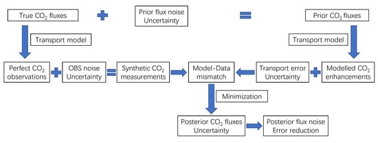
Figure 1.
Flow chart of the Observing System Simulation Experiment (OSSE) for urban CO inversion.
2. Data and Methods
2.1. TanSat-2 Configuration
The next-generation Chinese greenhouse gas monitoring satellite known as TanSat-2 is the continuation mission of China’s first carbon monitoring satellite, TanSat. TanSat-2 will fly at a medium-Earth orbit with an apogee of 7840 km and a perigee of 522 km (Figure 2). Previous studies indicate that more than 80% of anthropogenic CO emissions are concentrated in the region of 15°–55°N, which the apogee of TanSat-2 is placed over in order to measure most fossil fuel CO emissions. Three bands, O-A (0.747–0.773 m), CO and CH (1.590–1.675 m), and CO (1.990–2.095 m), provide continuous measurements of the atmospheric absorption spectrum of CO and CH, with an expected retrieval precision of less than 1 ppm and 8 ppb to account for clouds and aerosol loading. In addition, there is a visible band for measuring NO to identify and separate anthropogenic emissions from natural carbon fluxes. Overall, TanSat-2 includes normal push broom, target, and glint modes. A new cloud and aerosol polarization imager will be installed as well, providing additional information to reduce errors due to clouds and aerosol particles.
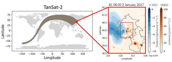
Figure 2.
TanSat-2 sampling trajectory and the simulated footprint of a cloud-free sample at 06:00 (UTC) 2 January 2017 over Beijing (BJ) with monthly mean ODIAC emissions. Footprint values are plotted on a logarithmic scale.
We simulated synthetic satellite measurements over BJ, JN, LA, and PR for four arbitrary clear-sky days in January and April 2017 (Figure 3). Following the same method described in Wu et al. (2023) [45], we used ERA5 total cloud cover reanalysis data at 0.250.25 resolution [57] to screen out samples contaminated by clouds while accounting for the organization of cloud distribution and the randomness of the impact of clouds and aerosol particles on satellite measurements. Of the more than one thousand individual samples over each city, our method identified 397 (BJ), 255 (JN), 217 (LA), and 307 (PR) samples as cloud-free in each city (Figure 3).
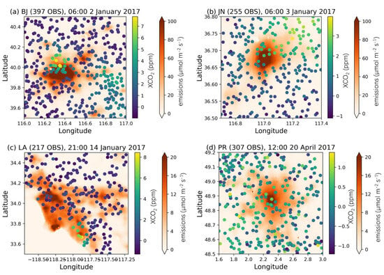
Figure 3.
Monthly mean ODIAC emissions and synthetic cloud-free CO samples over Beijing (a), Jinan (b), Los Angeles (c), and Paris (d).
2.2. Anthropogenic CO Emission Inventory
We used the Open-source Data Inventory for Anthropogenic CO (ODIAC, version 2020b) for monthly mean CO emissions from fossil fuels at a spatial resolution of 1 km × 1 km [58,59]. This data product uses satellite observations of night-time light and power plant profiles, including emission intensity and geographic location, to distribute CO emission estimates from fossil fuel combustion at the country level. Sources of systematic and random flux errors are due to spatial and temporal disaggregation that vary by emission sector at different scales (from national to urban) and uncertainties in the use of night-time light data as an emission proxy. We used ODIAC to define our broader study domains for urban areas and to ensure that anthropogenic source regions that lie outside the spatial extent of TanSat-2 were included (Figure 3). BJ (9.84 tCO s) and JN (1.63 tCO s) emissions of CO are concentrated in the city centre, with high emissions beyond 60 mol m s (Figure 3), home to about 21.54 and 8.7 million people. LA (3.67 tCO s) and PR (1.81 tCO s) show fewer CO emissions ranging from 10 to 20 mol m s (Figure 3), home to about 3.85 and 2.16 million people, where emissions are distributed with the expansion of city.
2.3. Atmospheric Transport Model
We used the column version of the Stochastic Time-Inverted Lagrangian Transport model (X-STILT) [60,61,62] to link surface CO fluxes to variations in atmospheric column CO at the locations of satellite sampling. X-STILT tracks the movement of air parcels backwards in time for 24 h. We applied a typical averaging kernel profile of OCO-2 and pressure weighting functions to the model fields to describe the footprints of satellite-based atmospheric CO measurements (Figure 2). The footprints describe the sensitivity of CO columns at the receptors (locations where the satellite observes the atmosphere) to upwind surface fluxes. In order to drive air parcels in X-STILT, we used meteorological data from the Global Forecast System with a horizontal resolution of 0.25 degrees (GFS0.25, https://www.ready.noaa.gov/data/archives/gfs0p25/ (accessed on 25 September 2023)) [63]. A total of 3000 air parcels evenly distributed from the surface to a 3 km height were released from the atmospheric column of each observation. We simulated footprints for the cloud-free observations sampled by TanSat-2. The sum of the convolution of the footprints and the ODIAC inventory represents the urban CO enhancements from upwind CO fluxes, as sampled by air parcels arriving at the locations of each sample.
2.4. Urban CO Inversion System
We followed the same method described in Wu et al. (2023) [45] to configure an urban CO inversion system with synthetic satellite measurements. Figure 1 describes the experimental design we followed to assess the theoretical ability of TanSat-2 sampling to quantify urban emissions of CO. We used the ODIAC emissions as the true state. The corresponding CO column enhancements were generated from the true fluxes using the X-STILT transport model. We added synthetic observation noise to each cloud-free scene based on simulations of cloud cover and aerosol loading. The random measurement errors ranged between −2 ppm to 2 ppm, with a standard deviation of 0.41 ppm to 0.54 ppm. We added an unbiased 20% random error to account for atmospheric transport errors [64,65]. Later in this paper, we examine the impacts of different transport errors (described by the observation error covariance matrix) on the error reduction of flux inversion.
Evaluating the ability to reduce a priori flux errors (including systematic and random errors) was the primary objective of this study. We assumed respective mean systematic and random flux error of 2 mol m s for the prior state [66,67]. The total systematic and random flux errors are constrained by the Chi-square test, which should be close to one (meaning that the posterior state is weighted by balancing the information from the data and the prior state) [16]. We used an eigenvalue decomposition method to generate a priori flux noise from the flux error covariance matrix, which is spatially correlated with an exponentially decaying function of the distance between emission grids. The spatial correlation length was assumed to be 10 km [68,69]. The vector of prior flux noise was calculated by multiplying the eigenvector of the flux error covariance matrix with a normal distribution vector characterizing the systematic and random flux errors.
We used the Maximum A Posteriori (MAP) inverse method [70,71,72], in which we solved for a posteriori CO emissions by minimizing a cost function [67] that describes the mismatch between the model-calculated enhancements and the measurements while accounting for a priori and measurement uncertainties. Minimizing the cost function results in the following expressions:
where and denote the a posteriori state of grid-based CO emissions and the associated error covariance matrix, and denote the a priori emissions and the associated error covariance matrix, the measurement vector includes the atmospheric CO column enhancements (with the associated errors described by the observation error covariance matrix , including measurement errors and atmospheric transport errors), and denotes the Jacobian matrix that describes the sensitivity of CO column enhancements to changes in surface CO emissions.
To evaluate the theoretical performance of TanSat-2 sampling on improving a priori knowledge of urban CO emissions, we used an error reduction metric () that takes into account differences between the a priori and a posteriori random flux errors [73]:
where the subscripts denote the diagonal elements of the error covariance matrices; the larger the value of , the more the uncertainty of CO emissions is reduced from the prior state due to assimilation of satellite data. Finally, we computed a metric for the overall correction of flux errors to account for the reduction of bias and random error in the flux estimates.
3. Results
3.1. Simulation of Satellite Sampling over Cities
We simulated synthetic TanSat-2 sampling over the cities of BJ, JN, LA, and PR on four arbitrary clear-sky days in January and April 2017 (Figure 3). The scattered distribution of cloud-free samples is due to the randomness of small-scale clouds, which are not resolved by the ERA5 cloud data. The differences in CO enhancements across the four cities (Figure 4a) are due to different emission levels and footprints associated with local meteorological conditions. The synthetic column CO enhancements (with measurement errors) in the four cities range from −2 ppm to 8 ppm, similar to previous studies [20,48,74,75]. The mean value of enhancements in BJ is 1.19 ppm, with a random error of 0.42 ppm (Figure 4b), resulting in a maximum signal-to-noise ratio of 2.8, followed by JN (2.1), LA (0.7), and PR (0.1). The signal-to-noise ratio of satellite data is an important indicator of flux error reduction, which shows significant correction in BJ and JN and negligible error reduction in PR (Figure 5). The sizable error reduction in each city is concentrated in the region with significant enhancement signals and high-density satellite sampling (Figure 3).
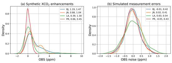
Figure 4.
Probability density of synthetic enhancements in Beijing (BJ), Jinan (JN), Los Angeles (LA), and Paris (PR) (a) along with the corresponding measurement errors (b). The values (in units of ppm) after the city names are the mean (first number) and standard deviation (second number).
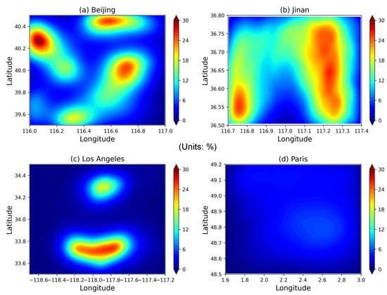
Figure 5.
Flux error reduction in Beijing (a), Jinan (b), Los Angeles (c), and Paris (d).
3.2. Comparison of Flux Inversion for Different Cities
Figures S1–S4 show the spatial distributions of the true, a priori, and a posteriori CO emissions and the associated flux noise in the cities of BJ, JN, LA, and PR. The a posteriori emissions optimized by the satellite data can retrieve the true integrated emissions for the four cities within 3% (BJ), 20% (JN), 31% (LA), and 30% (PR) from an a priori state of 13% (BJ), 65% (JN), 52% (LA), and 69% (PR) larger than the truth. The corresponding reductions in flux random errors are 28% (BJ), 19% (JN), 25% (LA), and 23% (PR). The reduced posterior flux noise due to flux correction illustrates that cloud-free satellite data can broadly retrieve the spatial structure and magnitude of the true emissions.
Figure 6 shows the urban CO column enhancements that correspond to the true, a priori, and a posteriori emissions. Certain satellite samples show a significant increase in CO (greater than 3) in BJ and LA, corresponding to a sizable reduction in flux errors in the two cities (Figure 5). The synthetic CO enhancements (synthetic OBS) in PR vary outside the range of truth (perfect OBS) due to the relatively low signal-to-noise ratio. Therefore, the reduction in flux error in PR is negligible (Figure 5). We evaluated the performance of inversion by comparing integrated urban CO emissions in the four cities (Figure 7). The bias correction ranges from 40% to 75%, with a 19% to 28% reduction in random flux error (Table 1). The overall correction (including bias and random error) ranges from 32% to 46% depending on the signal-to-noise ratio and the density of satellite sampling (due to clouds and aerosol loading) that can detect significant enhancement signals.
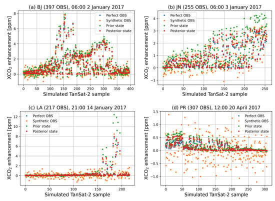
Figure 6.
Urban CO enhancements in Beijing (a), Jinan (b), Los Angeles (c), and Paris (d).
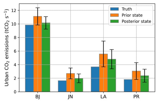
Figure 7.
Urban CO emissions in Beijing (BJ), Jinan (JN), Los Angeles (LA), and Paris (PR).

Table 1.
Reduction of flux bias and random error (RE) and overall correction (OC) of integrated urban CO emissions in Beijing (BJ), Jinan (JN), Los Angeles (LA), and Paris (PR); units are %.
3.3. Sensitivity to Systematic and Random Measurement Errors
We investigated the sensitivity of flux estimates to bias in satellite data for the medium-size city of JN (Figure 8a), which is a typical city in terms of the area of the city. A systematic measurement error of ±1 ppm would significantly degrade emission estimates inferred from the data, especially when the observation bias and the flux bias are in the same direction. A slight bias within −0.5 ppm in the data, in the opposite direction of a priori flux bias, is beneficial for improving the integrated estimate of CO emissions. Figure 8b shows the sensitivity of the flux error reduction to observation uncertainties, including atmospheric transport errors, under different resolutions of satellite sampling. The peak spatially-averaged error reduction is approximately 25% with an observation uncertainty of 0.5 ppm and the largest number of measurements. The lowest error reduction is for the minimum data availability (25 OBS) and a sampling resolution of 20 km. Moreover, the scenario of 4 km resolution (127 OBS) with 1 ppm observation uncertainty shows similar error reduction to the scenario of 8 km resolution (76 OBS), with a 0.75 ppm random error, indicating that better measurement precision can partially compensate for fewer measurements.
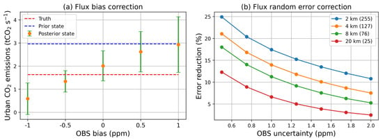
Figure 8.
Correction of flux bias with the change in observation bias in Jinan (a) and reduction of the spatially-averaged random flux error with the change in observation uncertainty under different sampling resolutions in Jinan (b). The numbers in parentheses are the number of observations.
4. Conclusions and Discussion
In this paper, we demonstrate that it is feasible to infer urban CO emissions from synthetic unbiased TanSat-2 data with a 19–28% correction for random flux errors. Because atmospheric column enhancements from urban CO emissions are less than 1% of the background concentration, the signal-to-noise ratio of satellite samples is important for determining error reduction in flux estimates. A systematic measurement error of ±1 ppm would significantly degrade emission estimates derived from the data. Improving the accuracy and precision of satellite samples can help to reduce uncertainties in urban CO emissions.
Although we evaluated the potential of using TanSat-2 data to detect anthropogenic CO emissions, there are additional limitations and uncertainties in applying these results to inversion experiments using real data [76]. As shown above, the reduction of flux errors is highly dependent on unbiased high-precision (less than 1 ppm random error) satellite measurements. However, satellite measurements are inevitably subject to bias due to the influence of clouds and aerosols. Data collected from ground-based remote sensing instruments (TCCON or EM27/SUN) are valuable to identify and correct larger-scale systematic errors. Deploying ground-based atmospheric remote sensing networks would help to correct regional systematic errors, while random measurement errors can be reduced by increasing the number of individual samples.
Column-averaged urban CO enhancements are typically less than 1% of the atmospheric background concentration (about 415 ppm). It has been suggested that estimating the regional background CO column concentration is important for quantifying the magnitude of urban CO enhancements due to net urban emissions, including anthropogenic and biospheric CO fluxes [77]. A range of methods have been investigated in different studies to quantify regional background values, such as calculating spatial CO gradients between upwind and downwind sites [12], solving for concentrations at the boundary as an additional unknown [78], averaging measurements over a latitude [79] or over surrounding areas that are relatively unaffected by urban emissions [20], simulating the background concentration with an atmospheric transport model [60], or deriving it from a two-step linear regression [26]. The choice of method for determining the background value depends on the specifics of each study, as all involve simplifications that affect the estimated urban emissions. Although the closed-loop experiment sidesteps this issue, it is necessary to consider additional uncertainties (assessment of wind direction and CO uptake by local ecosystems) associated with the calculation of the elevated in experiments with real data.
This study assumes unbiased and uncorrelated atmospheric transport errors. However, these errors are likely to be correlated at the sub-city scale [80]. Our assumptions likely result in the best-case scenario for error reduction that can be achieved by the TanSat-2 mission. Better understanding of atmospheric transport and a priori flux errors is essential to improving the accuracy and precision of a posteriori CO flux estimates. In addition, seasonal biospheric uptake of CO within and around cities weakens observed CO gradients, complicating the categorization of anthropogenic and natural fluxes [17,81,82,83]. Coupled assimilation of CO with other trace gases such as CO or NO can provide constraints, allowing fossil fuel emissions of CO in cities to be separated from natural fluxes [29,32].
Supplementary Materials
The following supporting information can be downloaded at: https://www.mdpi.com/article/10.3390/rs15204904/s1, Figure S1: Truth (a), prior state (b), posterior state (c), prior flux noise (prior state minus truth) (d), posterior flux noise (posterior state minus truth) (e), and flux correction (posterior minus prior state) (f) based on the cloud-free samples in Beijing at 06:00 (UTC) 02 JAN 2017. Values in parentheses are the total CO emissions within the domain and their uncertainty.; Figure S2: Same as Figure S1, but in Jinan at 06:00 (UTC) 03 JAN 2017; Figure S3: Same as Figure S1, but in Los Angeles at 21:00 (UTC) 14 JAN 2017; Figure S4: Same as Figure S1, but in Paris at 12:00 (UTC) 20 APR 2017.
Author Contributions
Conceptualization, K.W., D.Y. and Y.L.; Data curation, D.Y.; Formal analysis, K.W. and D.Y.; Funding acquisition, D.Y. and Y.L.; Methodology, K.W. and D.Y.; Visualization, K.W.; Writing—original draft, K.W. and D.Y.; Writing—review and editing, K.W., D.Y., Y.L., Z.C., M.Z., L.F. and P.I.P. All authors have read and agreed to the published version of the manuscript.
Funding
This work was supported by the National Key Research and Development Plan (2021YFB3901000) and the CAS Project for Young Scientists in Basic Research (Grant No.YSBR-037).
Data Availability Statement
The ODIAC emission inventory is available at http://dx.doi.org/10.17595/20170411.001 (accessed on 25 September 2023), hosted by the Center for Global Environmental Research, National Institute for Environmental Studies (https://db.cger.nies.go.jp/dataset/ODIAC/, accessed on 7 August 2023). The X-STILT model is available at https://github.com/uataq/X-STILT, accessed on 7 August 2023. Codes for this study are available upon request.
Acknowledgments
We thank Dien Wu at CIT for discussing the X-STILT transport model and Tom Oda at USRA for publishing the ODIAC emissions inventory.
Conflicts of Interest
The authors declare no conflict of interest.
References
- Butler, J.H.; Montzka, S.A. The NOAA annual greenhouse gas index (AGGI). NOAA Earth Syst. Res. Lab. 2016, 58. Available online: http://www.esrl.noaa.gov/gmd/aggi/aggi.html (accessed on 25 September 2023).
- Masson-Delmotte, V.; Zhai, P.; Pörtner, H.O.; Roberts, D.; Skea, J.; Shukla, P.R.; Pirani, A.; Moufouma-Okia, W.; Péan, C.; Pidcock, R.; et al. Global Warming of 1.5 °C: IPCC Special Report on Impacts of Global Warming of 1.5 °C above Pre-Industrial Levels in Context of Strengthening Response to Climate Change, Sustainable Development, and Efforts to Eradicate Poverty; Cambridge University Press: Cambridge, UK, 2022. [Google Scholar]
- Labzovskii, L.D.; Mak, H.W.L.; Kenea, S.T.; Rhee, J.S.; Lashkari, A.; Li, S.; Goo, T.Y.; Oh, Y.S.; Byun, Y.H. What can we learn about effectiveness of carbon reduction policies from interannual variability of fossil fuel CO2 emissions in East Asia? Environ. Sci. Policy 2019, 96, 132–140. [Google Scholar] [CrossRef]
- Masson-Delmotte, V.; Zhai, P.; Pirani, A.; Connors, S.L.; Péan, C.; Berger, S.; Caud, N.; Chen, Y.; Goldfarb, L.; Gomis, M.I.; et al. Climate Change 2021: The Physical Science Basis; Contribution of Working Group I to the Sixth Assessment Report of the Intergovernmental Panel on Climate Change; Cambridge University Press: Cambridge, UK, 2021; p. 2. [Google Scholar]
- Martins, T.; Barreto, A.C.; Souza, F.M.; Souza, A.M. Fossil fuels consumption and carbon dioxide emissions in G7 countries: Empirical evidence from ARDL bounds testing approach. Environ. Pollut. 2021, 291, 118093. [Google Scholar] [CrossRef] [PubMed]
- Le Quéré, C.; Peters, G.P.; Friedlingstein, P.; Andrew, R.M.; Canadell, J.G.; Davis, S.J.; Jackson, R.B.; Jones, M.W. Fossil CO2 emissions in the post-COVID-19 era. Nat. Clim. Change 2021, 11, 197–199. [Google Scholar] [CrossRef]
- Crisp, D.; Pollock, H.R.; Rosenberg, R.; Chapsky, L.; Lee, R.A.; Oyafuso, F.A.; Frankenberg, C.; O’Dell, C.W.; Bruegge, C.J.; Doran, G.B.; et al. The on-orbit performance of the Orbiting Carbon Observatory-2 (OCO-2) instrument and its radiometrically calibrated products. Atmos. Meas. Tech. 2017, 10, 59–81. [Google Scholar] [CrossRef]
- Lopez, M.; Schmidt, M.; Delmotte, M.; Colomb, A.; Gros, V.; Janssen, C.; Lehman, S.; Mondelain, D.; Perrussel, O.; Ramonet, M.; et al. CO, NOx and 13CO2 as tracers for fossil fuel CO2: Results from a pilot study in Paris during winter 2010. Atmos. Chem. Phys. 2013, 13, 7343–7358. [Google Scholar] [CrossRef]
- Bréon, F.; Broquet, G.; Puygrenier, V.; Chevallier, F.; Xueref-Remy, I.; Ramonet, M.; Dieudonné, E.; Lopez, M.; Schmidt, M.; Perrussel, O.; et al. An attempt at estimating Paris area CO2 emissions from atmospheric concentration measurements. Atmos. Chem. Phys. 2015, 15, 1707–1724. [Google Scholar] [CrossRef]
- Turner, A.J.; Shusterman, A.A.; McDonald, B.C.; Teige, V.; Harley, R.A.; Cohen, R.C. Network design for quantifying urban CO2 emissions: Assessing trade-offs between precision and network density. Atmos. Chem. Phys. 2016, 16, 13465–13475. [Google Scholar] [CrossRef]
- Helfter, C.; Tremper, A.H.; Halios, C.H.; Kotthaus, S.; Bjorkegren, A.; Grimmond, C.S.B.; Barlow, J.F.; Nemitz, E. Spatial and temporal variability of urban fluxes of methane, carbon monoxide and carbon dioxide above London, UK. Atmos. Chem. Phys. 2016, 16, 10543–10557. [Google Scholar] [CrossRef]
- Lauvaux, T.; Miles, N.L.; Deng, A.; Richardson, S.J.; Cambaliza, M.O.; Davis, K.J.; Gaudet, B.; Gurney, K.R.; Huang, J.; O’Keefe, D.; et al. High-resolution atmospheric inversion of urban CO2 emissions during the dormant season of the Indianapolis Flux Experiment (INFLUX). J. Geophys. Res. Atmos. 2016, 121, 5213–5236. [Google Scholar] [CrossRef]
- Davis, K.J.; Deng, A.; Lauvaux, T.; Miles, N.L.; Richardson, S.J.; Sarmiento, D.P.; Gurney, K.R.; Hardesty, R.M.; Bonin, T.A.; Brewer, A.W.; et al. The Indianapolis Flux Experiment (INFLUX): A test-bed for developing urban greenhouse gas emission measurements. Elem. Sci. Anth. 2017, 5, 21. [Google Scholar] [CrossRef] [PubMed]
- Verhulst, K.R.; Karion, A.; Kim, J.; Salameh, P.K.; Keeling, R.F.; Newman, S.; Miller, J.; Sloop, C.; Pongetti, T.; Rao, P.; et al. Carbon dioxide and methane measurements from the Los Angeles Megacity Carbon Project–Part 1: Calibration, urban enhancements, and uncertainty estimates. Atmos. Chem. Phys. 2017, 17, 8313–8341. [Google Scholar] [CrossRef] [PubMed]
- Sargent, M.; Barrera, Y.; Nehrkorn, T.; Hutyra, L.R.; Gately, C.K.; Jones, T.; McKain, K.; Sweeney, C.; Hegarty, J.; Hardiman, B.; et al. Anthropogenic and biogenic CO2 fluxes in the Boston urban region. Proc. Natl. Acad. Sci. USA 2018, 115, 7491–7496. [Google Scholar] [CrossRef] [PubMed]
- Kunik, L.; Mallia, D.V.; Gurney, K.R.; Mendoza, D.L.; Oda, T.; Lin, J.C. Bayesian inverse estimation of urban CO2 emissions: Results from a synthetic data simulation over Salt Lake City, UT. Elem. Sci. Anth. 2019, 7, 36. [Google Scholar] [CrossRef]
- Basu, S.; Lehman, S.J.; Miller, J.B.; Andrews, A.E.; Sweeney, C.; Gurney, K.R.; Xu, X.; Southon, J.; Tans, P.P. Estimating US fossil fuel CO2 emissions from measurements of 14C in atmospheric CO2. Proc. Natl. Acad. Sci. USA 2020, 117, 13300–13307. [Google Scholar] [CrossRef] [PubMed]
- Yokota, T.; Yoshida, Y.; Eguchi, N.; Ota, Y.; Tanaka, T.; Watanabe, H.; Maksyutov, S. Global concentrations of CO2 and CH4 retrieved from GOSAT: First preliminary results. Sola 2009, 5, 160–163. [Google Scholar] [CrossRef]
- Morino, I.; Uchino, O.; Inoue, M.; Yoshida, Y.; Yokota, T.; Wennberg, P.; Toon, G.; Wunch, D.; Roehl, C.; Notholt, J.; et al. Preliminary validation of column-averaged volume mixing ratios of carbon dioxide and methane retrieved from GOSAT short-wavelength infrared spectra. Atmos. Meas. Tech. 2011, 4, 1061–1076. [Google Scholar] [CrossRef]
- Kort, E.A.; Frankenberg, C.; Miller, C.E.; Oda, T. Space-based observations of megacity carbon dioxide. Geophys. Res. Lett. 2012, 39, L17806. [Google Scholar] [CrossRef]
- Janardanan, R.; Maksyutov, S.; Oda, T.; Saito, M.; Kaiser, J.W.; Ganshin, A.; Stohl, A.; Matsunaga, T.; Yoshida, Y.; Yokota, T. Comparing GOSAT observations of localized CO2 enhancements by large emitters with inventory-based estimates. Geophys. Res. Lett. 2016, 43, 3486–3493. [Google Scholar] [CrossRef]
- Hakkarainen, J.; Ialongo, I.; Tamminen, J. Direct space-based observations of anthropogenic CO2 emission areas from OCO-2. Geophys. Res. Lett. 2016, 43, 11–400. [Google Scholar] [CrossRef]
- Schwandner, F.M.; Gunson, M.R.; Miller, C.E.; Carn, S.A.; Eldering, A.; Krings, T.; Verhulst, K.R.; Schimel, D.S.; Nguyen, H.M.; Crisp, D.; et al. Spaceborne detection of localized carbon dioxide sources. Science 2017, 358, eaam5782. [Google Scholar] [CrossRef] [PubMed]
- Eldering, A.; Wennberg, P.O.; Crisp, D.; Schimel, D.S.; Gunson, M.R.; Chatterjee, A.; Liu, J.; Schwandner, F.M.; Sun, Y.; O’Dell, C.W.; et al. The Orbiting Carbon Observatory-2 early science investigations of regional carbon dioxide fluxes. Science 2017, 358, eaam5745. [Google Scholar] [CrossRef] [PubMed]
- Chevallier, F.; Broquet, G.; Zheng, B.; Ciais, P.; Eldering, A. Large CO2 emitters as seen from satellite: Comparison to a gridded global emission inventory. Geophys. Res. Lett. 2022, 49, e2021GL097540. [Google Scholar] [CrossRef] [PubMed]
- Ye, X.; Lauvaux, T.; Kort, E.A.; Oda, T.; Feng, S.; Lin, J.C.; Yang, E.G.; Wu, D. Constraining fossil fuel CO2 emissions from urban area using OCO-2 observations of total column CO2. J. Geophys. Res. Atmos. 2020, 125, e2019JD030528. [Google Scholar] [CrossRef]
- Zheng, B.; Chevallier, F.; Ciais, P.; Broquet, G.; Wang, Y.; Lian, J.; Zhao, Y. Observing carbon dioxide emissions over China’s cities and industrial areas with the Orbiting Carbon Observatory-2. Atmos. Chem. Phys. 2020, 20, 8501–8510. [Google Scholar] [CrossRef]
- Lei, R.; Feng, S.; Danjou, A.; Broquet, G.; Wu, D.; Lin, J.C.; O’Dell, C.W.; Lauvaux, T. Fossil fuel CO2 emissions over metropolitan areas from space: A multi-model analysis of OCO-2 data over Lahore, Pakistan. Remote Sens. Environ. 2021, 264, 112625. [Google Scholar] [CrossRef]
- Reuter, M.; Buchwitz, M.; Hilboll, A.; Richter, A.; Schneising, O.; Hilker, M.; Heymann, J.; Bovensmann, H.; Burrows, J. Decreasing emissions of NOx relative to CO2 in East Asia inferred from satellite observations. Nat. Geosci. 2014, 7, 792–795. [Google Scholar] [CrossRef]
- Konovalov, I.B.; Berezin, E.V.; Ciais, P.; Broquet, G.; Zhuravlev, R.V.; Janssens-Maenhout, G. Estimation of fossil-fuel CO2 emissions using satellite measurements of “proxy” species. Atmos. Chem. Phys. 2016, 16, 13509–13540. [Google Scholar] [CrossRef]
- Goldberg, D.L.; Lu, Z.; Oda, T.; Lamsal, L.N.; Liu, F.; Griffin, D.; McLinden, C.A.; Krotkov, N.A.; Duncan, B.N.; Streets, D.G. Exploiting OMI NO2 satellite observations to infer fossil-fuel CO2 emissions from US megacities. Sci. Total Environ. 2019, 695, 133805. [Google Scholar] [CrossRef]
- Reuter, M.; Buchwitz, M.; Schneising, O.; Krautwurst, S.; O’Dell, C.W.; Richter, A.; Bovensmann, H.; Burrows, J.P. Towards monitoring localized CO2 emissions from space: Co-located regional CO2 and NO2 enhancements observed by the OCO-2 and S5P satellites. Atmos. Chem. Phys. 2019, 19, 9371–9383. [Google Scholar] [CrossRef]
- Hakkarainen, J.; Szeląg, M.E.; Ialongo, I.; Retscher, C.; Oda, T.; Crisp, D. Analyzing nitrogen oxides to carbon dioxide emission ratios from space: A case study of Matimba Power Station in South Africa. Atmos. Environ. X 2021, 10, 100110. [Google Scholar] [CrossRef]
- Park, H.; Jeong, S.; Park, H.; Labzovskii, L.D.; Bowman, K.W. An assessment of emission characteristics of Northern Hemisphere cities using spaceborne observations of CO2, CO, and NO2. Remote Sens. Environ. 2021, 254, 112246. [Google Scholar] [CrossRef]
- Finch, D.P.; Palmer, P.I.; Zhang, T. Automated detection of atmospheric NO2 plumes from satellite data: A tool to help infer anthropogenic combustion emissions. Atmos. Meas. Tech. 2022, 15, 721–733. [Google Scholar] [CrossRef]
- Massie, S.T.; Sebastian Schmidt, K.; Eldering, A.; Crisp, D. Observational evidence of 3-D cloud effects in OCO-2 CO2 retrievals. J. Geophys. Res. Atmos. 2017, 122, 7064–7085. [Google Scholar] [CrossRef]
- O’Dell, C.W.; Eldering, A.; Wennberg, P.O.; Crisp, D.; Gunson, M.R.; Fisher, B.; Frankenberg, C.; Kiel, M.; Lindqvist, H.; Mandrake, L.; et al. Improved retrievals of carbon dioxide from Orbiting Carbon Observatory-2 with the version 8 ACOS algorithm. Atmos. Meas. Tech. 2018, 11, 6539–6576. [Google Scholar] [CrossRef]
- Suto, H.; Kataoka, F.; Kikuchi, N.; Knuteson, R.O.; Butz, A.; Haun, M.; Buijs, H.; Shiomi, K.; Imai, H.; Kuze, A. Thermal and near-infrared sensor for carbon observation Fourier transform spectrometer-2 (TANSO-FTS-2) on the Greenhouse gases Observing SATellite-2 (GOSAT-2) during its first year in orbit. Atmos. Meas. Tech. 2021, 14, 2013–2039. [Google Scholar] [CrossRef]
- Cai, Z.; Liu, Y.; Yang, D. Analysis of XCO 2 retrieval sensitivity using simulated Chinese Carbon Satellite (TanSat) measurements. Sci. China Earth Sci. 2014, 57, 1919–1928. [Google Scholar] [CrossRef]
- Liu, Y.; Wang, J.; Yao, L.; Chen, X.; Cai, Z.; Yang, D.; Yin, Z.; Gu, S.; Tian, L.; Lu, N.; et al. The TanSat mission: Preliminary global observations. Sci. Bull. 2018, 63, 1200–1207. [Google Scholar] [CrossRef]
- Yang, D.; Liu, Y.; Cai, Z.; Chen, X.; Yao, L.; Lu, D. First global carbon dioxide maps produced from TanSat measurements. Adv. Atmos. Sci. 2018, 35, 621–623. [Google Scholar] [CrossRef]
- Yang, D.; Boesch, H.; Liu, Y.; Somkuti, P.; Cai, Z.; Chen, X.; Di Noia, A.; Lin, C.; Lu, N.; Lyu, D.; et al. Toward high precision XCO 2 retrievals from TanSat observations: Retrieval improvement and validation against TCCON measurements. J. Geophys. Res. Atmos. 2020, 125, e2020JD032794. [Google Scholar] [CrossRef]
- Bertaux, J.L.; Hauchecorne, A.; Lefèvre, F.; Bréon, F.M.; Blanot, L.; Jouglet, D.; Lafrique, P.; Akaev, P. The use of the 1.27 μm O2 absorption band for greenhouse gas monitoring from space and application to MicroCarb. Atmos. Meas. Tech. 2020, 13, 3329–3374. [Google Scholar] [CrossRef]
- Jouglet, D.; Landiech, P.; Breon, F.M.; The MicroCarb Team. MicroCarb, first European program for CO2 monitoring: Nearing development conclusion before launch. In Proceedings of the IWGGMS-17 Conference, Online, 14–17 June 2021. [Google Scholar]
- Wu, K.; Palmer, P.I.; Wu, D.; Jouglet, D.; Feng, L.; Oda, T. Theoretical assessment of the ability of the MicroCarb satellite city-scan observing mode to estimate urban CO2 emissions. Atmos. Meas. Tech. 2023, 16, 581–602. [Google Scholar] [CrossRef]
- Kuhlmann, G.; Brunner, D.; Broquet, G.; Meijer, Y. Quantifying CO2 emissions of a city with the Copernicus Anthropogenic CO2 Monitoring satellite mission. Atmos. Meas. Tech. 2020, 13, 6733–6754. [Google Scholar] [CrossRef]
- Sierk, B.; Fernandez, V.; Bézy, J.L.; Meijer, Y.; Durand, Y.; Courrèges-Lacoste, G.B.; Pachot, C.; Löscher, A.; Nett, H.; Minoglou, K.; et al. The Copernicus CO2M mission for monitoring anthropogenic carbon dioxide emissions from space. In Proceedings of the International Conference on Space Optics—ICSO 2020, Online, 30 March–2 April 2020; Cugny, B., Sodnik, Z., Karafolas, N., Eds.; International Society for Optics and Photonics (SPIE): Bellingham, WA, USA, 2021; Volume 11852, p. 118523M. [Google Scholar]
- Kiel, M.; Eldering, A.; Roten, D.D.; Lin, J.C.; Feng, S.; Lei, R.; Lauvaux, T.; Oda, T.; Roehl, C.M.; Blavier, J.F.; et al. Urban-focused satellite CO2 observations from the Orbiting Carbon Observatory-3: A first look at the Los Angeles megacity. Remote Sens. Environ. 2021, 258, 112314. [Google Scholar] [CrossRef]
- Eldering, A.; Taylor, T.E.; O’Dell, C.W.; Pavlick, R. The OCO-3 mission: Measurement objectives and expected performance based on 1 year of simulated data. Atmos. Meas. Tech. 2019, 12, 2341–2370. [Google Scholar] [CrossRef]
- Taylor, T.E.; Eldering, A.; Merrelli, A.; Kiel, M.; Somkuti, P.; Cheng, C.; Rosenberg, R.; Fisher, B.; Crisp, D.; Basilio, R.; et al. OCO-3 early mission operations and initial (vEarly) XCO 2 and SIF retrievals. Remote Sens. Environ. 2020, 251, 112032. [Google Scholar] [CrossRef]
- Wu, D.; Lin, J.C.; Oda, T.; Kort, E.A. Space-based quantification of per capita CO2 emissions from cities. Environ. Res. Lett. 2020, 15, 035004. [Google Scholar] [CrossRef]
- Yang, E.G.; Kort, E.A.; Wu, D.; Lin, J.C.; Oda, T.; Ye, X.; Lauvaux, T. Using space-based observations and Lagrangian modeling to evaluate urban carbon dioxide emissions in the Middle East. J. Geophys. Res. Atmos. 2020, 125, e2019JD031922. [Google Scholar] [CrossRef] [PubMed]
- Wunch, D.; Toon, G.C.; Blavier, J.F.L.; Washenfelder, R.A.; Notholt, J.; Connor, B.J.; Griffith, D.W.; Sherlock, V.; Wennberg, P.O. The total carbon column observing network. Philos. Trans. R. Soc. A Math. Phys. Eng. Sci. 2011, 369, 2087–2112. [Google Scholar] [CrossRef]
- Wunch, D.; Wennberg, P.O.; Osterman, G.; Fisher, B.; Naylor, B.; Roehl, C.M.; O’Dell, C.; Mandrake, L.; Viatte, C.; Kiel, M.; et al. Comparisons of the orbiting carbon observatory-2 (OCO-2) X CO2 measurements with TCCON. Atmos. Meas. Tech. 2017, 10, 2209–2238. [Google Scholar] [CrossRef]
- Zhou, M.; Ni, Q.; Cai, Z.; Langerock, B.; Nan, W.; Yang, Y.; Che, K.; Yang, D.; Wang, T.; Liu, Y.; et al. CO2 in Beijing and Xianghe Observed by Ground-Based FTIR Column Measurements and Validation to OCO-2/3 Satellite Observations. Remote Sens. 2022, 14, 3769. [Google Scholar] [CrossRef]
- Cai, Z.; Sun, K.; Yang, D.; Liu, Y.; Yao, L.; Lin, C.; Liu, X. On-Orbit Characterization of TanSat Instrument Line Shape Using Observed Solar Spectra. Remote Sens. 2022, 14, 3334. [Google Scholar] [CrossRef]
- Hersbach, H.; Bell, B.; Berrisford, P.; Biavati, G.; Horányi, A.; Muñoz Sabater, J.; Nicolas, J.; Peubey, C.; Radu, R.; Rozum, I.; et al. ERA5 hourly data on single levels from 1979 to present. Copernic. Clim. Change Serv. Clim. Data Store 2018, 10. [Google Scholar] [CrossRef]
- Oda, T.; Maksyutov, S. A very high-resolution (1 km × 1 km) global fossil fuel CO2 emission inventory derived using a point source database and satellite observations of nighttime lights. Atmos. Chem. Phys. 2011, 11, 543. [Google Scholar] [CrossRef]
- Oda, T.; Maksyutov, S.; Andres, R.J. The Open-source Data Inventory for Anthropogenic CO2, version 2016 (ODIAC2016): A global monthly fossil fuel CO2 gridded emissions data product for tracer transport simulations and surface flux inversions. Earth Syst. Sci. Data 2018, 10, 87–107. [Google Scholar] [CrossRef] [PubMed]
- Wu, D.; Lin, J.C.; Fasoli, B.; Oda, T.; Ye, X.; Lauvaux, T.; Yang, E.G.; Kort, E.A. A Lagrangian approach towards extracting signals of urban CO2 emissions from satellite observations of atmospheric column CO2 (XCO2): X-Stochastic Time-Inverted Lagrangian Transport model (“X-STILT v1”). Geosci. Model Dev. 2018, 11, 4843–4871. [Google Scholar] [CrossRef]
- Fasoli, B.; Lin, J.C.; Bowling, D.R.; Mitchell, L.; Mendoza, D. Simulating atmospheric tracer concentrations for spatially distributed receptors: Updates to the Stochastic Time-Inverted Lagrangian Transport model’s R interface (STILT-R version 2). Geosci. Model Dev. 2018, 11, 2813–2824. [Google Scholar] [CrossRef]
- Lin, J.; Gerbig, C.; Wofsy, S.; Andrews, A.; Daube, B.; Davis, K.; Grainger, C. A near-field tool for simulating the upstream influence of atmospheric observations: The Stochastic Time-Inverted Lagrangian Transport (STILT) model. J. Geophys. Res. Atmos. 2003, 108, 4493. [Google Scholar] [CrossRef]
- NCEP. 0.25 Degree Global Forecast Grids Historical Archive (Research Data Archive at the National Center for Atmospheric Research, Computational and Information Systems Laboratory; National Centers for Environmental Prediction/National Weather Service/NOAA/US Department of Commerce: Boulder, CO, USA, 2015. [Google Scholar]
- Deng, A.; Lauvaux, T.; Davis, K.J.; Gaudet, B.J.; Miles, N.L.; Richardson, S.J.; Wu, K.; Sarmiento, D.P.; Hardesty, R.M.; Bonin, T.A.; et al. Toward reduced transport errors in a high resolution urban CO2 inversion system. Elem. Sci. Anth. 2017, 5, 20. [Google Scholar] [CrossRef]
- Lauvaux, T.; Díaz-Isaac, L.I.; Bocquet, M.; Bousserez, N. Diagnosing spatial error structures in CO2 mole fractions and XCO2 column mole fractions from atmospheric transport. Atmos. Chem. Phys. 2019, 19, 12007–12024. [Google Scholar] [CrossRef]
- Oda, T.; Bun, R.; Kinakh, V.; Topylko, P.; Halushchak, M.; Marland, G.; Lauvaux, T.; Jonas, M.; Maksyutov, S.; Nahorski, Z.; et al. Errors and uncertainties in a gridded carbon dioxide emissions inventory. Mitig. Adapt. Strateg. Glob. Change 2019, 24, 1007–1050. [Google Scholar] [CrossRef]
- Wu, K.; Lauvaux, T.; Davis, K.J.; Deng, A.; Coto, I.L.; Gurney, K.R.; Patarasuk, R. Joint inverse estimation of fossil fuel and biogenic CO2 fluxes in an urban environment: An observing system simulation experiment to assess the impact of multiple uncertainties. Elem. Sci. Anth. 2018, 6, 116, D21304. [Google Scholar] [CrossRef]
- Saide, P.; Bocquet, M.; Osses, A.; Gallardo, L. Constraining surface emissions of air pollutants using inverse modelling: Method intercomparison and a new two-step two-scale regularization approach. Tellus B 2011, 63, 360–370. [Google Scholar] [CrossRef]
- Wu, L.; Bocquet, M.; Lauvaux, T.; Chevallier, F.; Rayner, P.; Davis, K. Optimal representation of source-sink fluxes for mesoscale carbon dioxide inversion with synthetic data. J. Geophys. Res. Atmos. 2011, 116. [Google Scholar] [CrossRef]
- Enting, I.G. Inverse Problems in Atmospheric Constituent Transport; Cambridge University Press: Cambridge, UK, 2002. [Google Scholar]
- Tarantola, A. Inverse Problem Theory and Methods for Model Parameter Estimation; SIAM: Philadelphia, PA, USA, 2004. [Google Scholar]
- Feng, L.; Palmer, P.; Bösch, H.; Dance, S. Estimating surface CO2 fluxes from space-borne CO2 dry air mole fraction observations using an ensemble Kalman Filter. Atmos. Chem. Phys. 2009, 9, 2619–2633. [Google Scholar] [CrossRef]
- Palmer, P.I.; Barnett, J.; Eyre, J.; Healy, S. A nonlinear optimal estimation inverse method for radio occultation measurements of temperature, humidity, and surface pressure. J. Geophys. Res. Atmos. 2000, 105, 17513–17526. [Google Scholar] [CrossRef]
- Hedelius, J.K.; Feng, S.; Roehl, C.M.; Wunch, D.; Hillyard, P.W.; Podolske, J.R.; Iraci, L.T.; Patarasuk, R.; Rao, P.; O’Keeffe, D.; et al. Emissions and topographic effects on column CO2 (XCO2) variations, with a focus on the Southern California Megacity. J. Geophys. Res. Atmos. 2017, 122, 7200–7215. [Google Scholar] [CrossRef]
- Hedelius, J.K.; Liu, J.; Oda, T.; Maksyutov, S.; Roehl, C.M.; Iraci, L.T.; Podolske, J.R.; Hillyard, P.W.; Liang, J.; Gurney, K.R.; et al. Southern California megacity CO2, CH4, and CO flux estimates using ground-and space-based remote sensing and a Lagrangian model. Atmos. Chem. Phys. 2018, 18, 16271–16291. [Google Scholar] [CrossRef]
- Broquet, G.; Bréon, F.M.; Renault, E.; Buchwitz, M.; Reuter, M.; Bovensmann, H.; Chevallier, F.; Wu, L.; Ciais, P. The potential of satellite spectro-imagery for monitoring CO2 emissions from large cities. Atmos. Meas. Tech. 2018, 11, 681–708. [Google Scholar] [CrossRef]
- Schuh, A.E.; Otte, M.; Lauvaux, T.; Oda, T. Far-field biogenic and anthropogenic emissions as a dominant source of variability in local urban carbon budgets: A global high-resolution model study with implications for satellite remote sensing. Remote Sens. Environ. 2021, 262, 112473. [Google Scholar] [CrossRef]
- Nickless, A.; Rayner, P.J.; Scholes, R.J.; Engelbrecht, F.; Erni, B. An atmospheric inversion over the city of Cape Town: Sensitivity analyses. Atmos. Chem. Phys. 2019, 19, 7789–7816. [Google Scholar] [CrossRef]
- Hakkarainen, J.; Ialongo, I.; Maksyutov, S.; Crisp, D. Analysis of four years of global XCO2 anomalies as seen by orbiting carbon observatory-2. Remote Sens. 2019, 11, 850. [Google Scholar] [CrossRef]
- Varentsov, A.I.; Stepanenko, V.M.; Konstantinov, P.I. High-resolution simulation of particle transport in the urban atmospheric boundary layer. IOP Conf. Ser. Earth Environ. Sci. 2019, 386, 012045. [Google Scholar] [CrossRef]
- Turnbull, J.C.; Sweeney, C.; Karion, A.; Newberger, T.; Lehman, S.J.; Tans, P.P.; Davis, K.J.; Lauvaux, T.; Miles, N.L.; Richardson, S.J.; et al. Toward quantification and source sector identification of fossil fuel CO2 emissions from an urban area: Results from the INFLUX experiment. J. Geophys. Res. Atmos. 2015, 120, 292–312. [Google Scholar] [CrossRef]
- Miller, J.B.; Lehman, S.J.; Verhulst, K.R.; Miller, C.E.; Duren, R.M.; Yadav, V.; Newman, S.; Sloop, C.D. Large and seasonally varying biospheric CO2 fluxes in the Los Angeles megacity revealed by atmospheric radiocarbon. Proc. Natl. Acad. Sci. USA 2020, 117, 26681–26687. [Google Scholar] [CrossRef]
- Wu, K.; Davis, K.J.; Miles, N.L.; Richardson, S.J.; Lauvaux, T.; Sarmiento, D.P.; Balashov, N.V.; Keller, K.; Turnbull, J.; Gurney, K.R.; et al. Source decomposition of eddy-covariance CO2 flux measurements for evaluating a high-resolution urban CO2 emissions inventory. Environ. Res. Lett. 2022, 17, 074035. [Google Scholar] [CrossRef]
Disclaimer/Publisher’s Note: The statements, opinions and data contained in all publications are solely those of the individual author(s) and contributor(s) and not of MDPI and/or the editor(s). MDPI and/or the editor(s) disclaim responsibility for any injury to people or property resulting from any ideas, methods, instructions or products referred to in the content. |
© 2023 by the authors. Licensee MDPI, Basel, Switzerland. This article is an open access article distributed under the terms and conditions of the Creative Commons Attribution (CC BY) license (https://creativecommons.org/licenses/by/4.0/).