PM_2.5 Estimation in Day/Night-Time from Himawari-8 Infrared Bands via a Deep Learning Neural Network

Abstract

Satellite-based PM_2.5 estimation is an effective means to achieve large-scale and long-term PM_2.5 monitoring and investigation. Currently, most of methods retrieve PM_2.5 from satellite-derived aerosol optical depth (AOD) or top-of-atmosphere reflectance (TOAR) during daytime. A few algorithms are also developed to retrieve nighttime PM_2.5 from the satellite day–night band and the accuracy is greatly limited by moonlight and artificial light sources. In this study, we utilize the properties of absorption pollutants in infrared spectrum to estimate PM_2.5 concentrations from satellite infrared data, thus achieve the PM_2.5 estimation in both day and night. Himawari-8 infrared bands data are used for PM_2.5 estimation by a specifically designed neural network and loss function. Quantitative results show the satellite derived PM_2.5 concentrations correlates with ground-based data well with R² of 0.79 and RMSE of 15.43 μg · m⁻³ for hourly PM_2.5 estimation. Spatiotemporal distributions of model-estimated PM_2.5 over China are also analyzed, and exhibit a highly consistent with ground-based measurements. Dust storms, heavy air pollution and fire smoke events are examined to further demonstrate the efficacy of our model. Our method not only circumvents the intermediate retrievals of AOD, but also enables consistent estimation of PM_2.5 concentrations during daytime and nighttime in real-time monitoring.

1. Introduction

Atmospheric particulate matter with an aerodynamic diameter less than 2.5 μm is known as fine particle matter (PM_2.5), which has been proven to have strong correlations with human health and Earth’s climate. Past decades have seen the rapid development and urbanization in developing countries. PM_2.5 has become a major pollutant in those countries such as China. Accurate PM_2.5 concentration monitoring and estimation has become an increasingly serious and worldwide concern.

The ground-based monitoring site is the most straightforward way to measure ground level PM_2.5 concentrations, which is generally grouped into air quality monitoring network. For example, China and India established PM_2.5 ground-based monitoring network in 2012 and 2015, respectively, and the number of monitoring sites continues to increase [1,2]. However, restrictions such as sparse spatial coverage and lack of historical data limit our ability to construct a spatiotemporally coherent mapping of PM_2.5, which is particularly useful in large-scale and long-term evaluation.

Relying on satellite remote sensing data to estimate ground-level PM_2.5 concentrations is an alternative to overcome the limitations of ground-based monitoring sites, which results in a broader spatiotemporal coverage estimation [3]. Due to the correlations between PM_2.5 concentration and aerosol optical depth (AOD) [4], quite a lot of studies on PM_2.5 estimation have been conducted. The most fundamental way is to model the dependency of PM_2.5 and satellite AOD products based on the theoretical relationship between them [5]. Some physical methods [6,7] that characterize the aerosol spatiotemporal and vertical distributions and a few chemical transport models simulations joint approaches [8,9,10] are developed subsequently. The accuracy of these methods tends to be limited due to the complicated transmission and formation process of PM_2.5. Therefore, statistical methods, which directly establish the PM_2.5-AOD relationship, have become the mainstream in PM_2.5 estimation, including considerable linear and non-linear statistical models [11,12,13]. To better account for the spatiotemporal variability of the relationship and improve the generalization performance of models, a number of advanced statistical models incorporating many extra related variables, e.g., meteorological variables and other ancillary variables, are developed [14,15,16,17,18,19,20,21]. Moreover, some ensemble and two-stage models are proposed to further improve the performance [22,23,24,25]. Recently, with the rapid development of machine learning and deep learning techniques, several machine learning-based algorithms are applied to satellite-based PM_2.5 estimation owing to its strong feature representation and nonlinear fitting capabilities, such as random forest [26,27,28], extreme gradient boosting [23], deep belief network [29], neural network model [30,31,32], etc.

However, despite their promising performance on different kinds of satellite data, there are two underlying limitations to existing PM_2.5 estimation methods. First, most of these studies are based on the satellite-retrieved AOD products incorporating other predictors to estimate PM_2.5 concentrations, thus the errors and uncertainties in AOD retrieval process would be inevitably introduced in PM_2.5 estimation, especially in heavily polluted areas with sparse vegetation [33]. Second, although there are some studies focusing on estimation from top-of-the-atmosphere reflectance (TOAR) data to circumvent the intermediate AOD retrieval process [34,35,36], neither AOD-based nor TOAR-based methods can estimate PM_2.5 concentrations at nighttime. Although there are some methods that depend on multisource AOD products [37,38] or use nighttime light imagery to retrieve nighttime PM_2.5 concentrations, such as using the day–night band (DNB) of the Visible Infrared Imaging Radiometer Suite (VIIRS) [39,40,41], Defense Meteorological Satellite Program/Operational Linescan System (DMSP/OLS) [42,43], or the LJ1-01 satellite [44,45]. They are usually limited by moonlight conditions and artificial light sources, and the study areas are often restricted. Moreover, different methods are needed for the estimation of daytime and nighttime PM_2.5. In addition, the polar-orbiting satellites have a relative long revisit cycle, which greatly limit the time continuity of large-scale PM_2.5 data and timelines of real-time monitoring.

The aim of this study is to demonstrate the potential of using the geostationary satellite infrared bands data, along with some meteorological parameters, to estimate large-scale and hourly PM_2.5 concentrations during both daytime and nighttime via a deep-learning-based model. Due to some pollutants such as sulfur dioxide (SO₂), nitrogen oxides (NO_x), carbon monoxide (CO) and ozone (O₃) having positive correlations with PM_2.5 [35], and these pollutants having absorption characteristics in infrared spectrum [46,47], the possibility of estimating PM_2.5 concentrations from satellite infrared bands data directly is therefore suggested. Note that this study is based on the absorption characteristics of some PM_2.5-related pollutants in the infrared spectrum to directly estimate the PM_2.5 concentrations. Given the infrared bands can operate day and night and are independent of solar radiation, it is possible to estimate full-time PM_2.5 concentrations from satellite infrared data regardless of daytime or nighttime.

In this study, an attempt is made to use Himawari-8 infrared bands data, also with meteorological variables, to estimate full-time PM_2.5 concentrations over mainland China via a neural network. A specific network architecture and loss function are designed for accurate estimation. The model performance is evaluated by cross-validation method with several statistical metrics. Spatiotemporal variations in model-estimated PM_2.5 concentrations over China and three major polluted areas that have frequent and periodic heavy pollution are analyzed. Moreover, three kinds of environmental pollution incidents, namely heavy air pollution cases, dust storms and fire smoke events, are examined to further demonstrate the efficacy of our model.

Provided with the vast geographical range and highly variable air quality conditions in China, we choose mainland China as our study area. The datasets used in this study mainly consist of satellite data, ground-based PM_2.5 concentration measurements, and several meteorological variables that have significant correlations with PM_2.5.

1.1. Satellite Data

Himawari-8 (H8) is a geostationary meteorological satellite operated by the Japan Meteorological Agency (JMA). The Advanced Himawari Imager (AHI) onboard H8 is a new payload for dedicated meteorological mission. It has 16 spectral bands: three in the visible, three in the near-infrared, and ten in the infrared bands. The AHI can produce images with a resolution down to 500 m and can complete a full-disk scan in every 10 min. More details about functions and specifications for each band can be found in [48]. In this study, 10 infrared bands (band 7–16, spectral range from 3.9 μm to 13.3 μm with a spatial resolution of 2 km) from 1 July 2019 to 1 July 2020 over mainland China are used. To match the temporal resolution of data from other sources, only hourly data are used. Brightness temperature values of the ten infrared bands are used as part of input in the neural network. Quality control is performed first to filter pixels with filling values. Cloud masks from [49] are applied to remove cloud-contaminated pixels before training.

1.2. Ground-Based PM_2.5 Concentration Measurements

The China National Environmental Monitoring Center (CNEMC) has established the PM_2.5 ground-based monitoring network at the end of 2012. There are about 2000 sites over mainland China as of 1 January 2021. It can provide hourly and daily ground-based concentration measurements of SO₂, NO₂, CO, O₃, PM₁₀, PM_2.5 and the air quality index (AQI). In this study, hourly PM_2.5 measurements from 1 July 2019 to 1 July 2020 are used as the true value of PM_2.5 concentrations for neural network training and testing. Additionally, cautious quality control processes are performed to ensure data accuracy and quality, including:

• Missing values in a site record lasting three hours or less are infilled by linear interpolation to help reduce the noise;
• Repeated values that last for more than four consecutive hours and implausible zeros are removed;
• Values beyond the concurrent PM₁₀ measurements in a site are removed;
• Regional consistency checks are performed by comparing sites with their neighboring sites to remove outliers.

1.3. Meteorological Variables

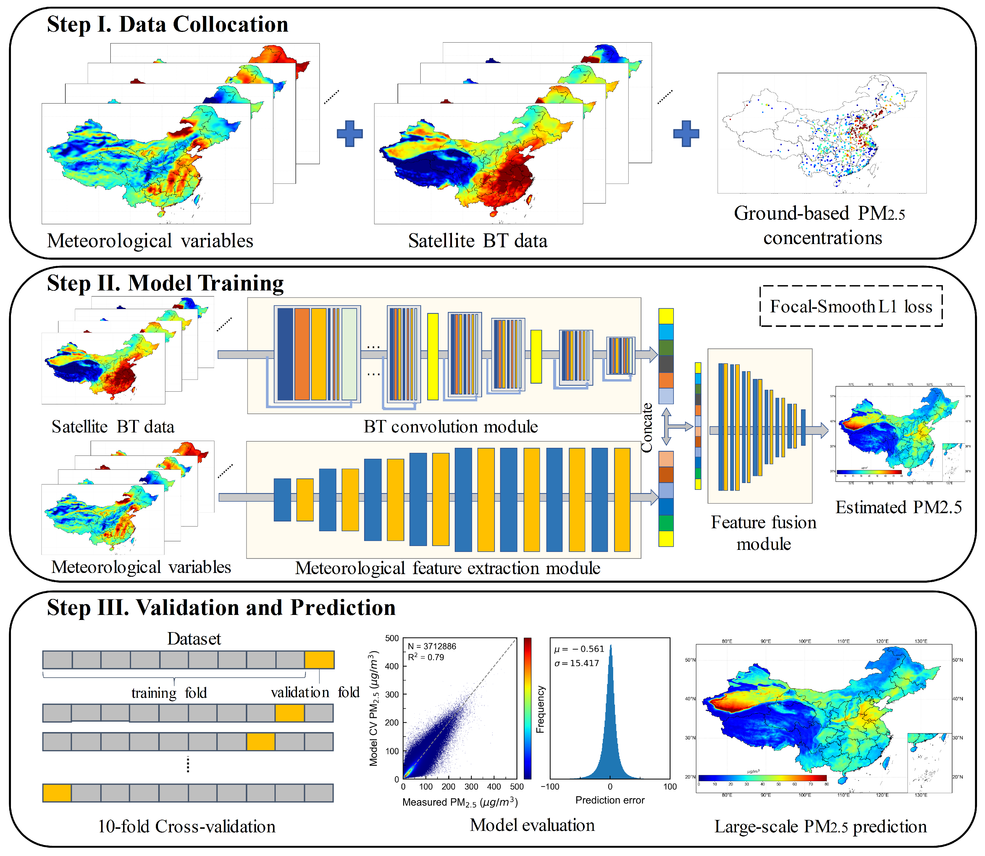
Several meteorological variables have been revealed to have significant correlations with PM_2.5 concentrations and are therefore selected as ancillary variables in satellite-based PM_2.5 estimation [50,51]. In this study, the 10 m u/v-components of neutral wind (at a height of 10 m above the surface of the Earth, the same applies hereinafter), 2 m temperature, 2 m dewpoint temperature, planetary boundary layer height, evaporation, skin temperature, surface pressure, total column water, total column ozone and total precipitation from ERA5 reanalysis data [52], with a temporal resolution of one hour and spatial resolution of 0.25° × 0.25°, are used as part of the input in the neural network to concurrently estimate PM_2.5 concentration. These parameters, which reflect the state of the atmosphere, may have influences on aerosols and also the transmission and formation process of PM_2.5.

Due to different spatial resolution from H8 data, these data are regridded to the H8 pixels grid with the cubic interpolation method. Moreover, because all the meteorological variables have different units and magnitudes, these variables need to be normalized before feeding into the neural network to have the same mean and deviation.

2. Methodology

In this study, we propose a deep-learning-based method to estimation PM_2.5 concentrations from the satellite infrared data incorporating the above mentioned meteorological variables. The overall route of our method consists of three parts, as shown in Figure 1. A specific network architecture and loss function are designed for accurate estimation, which can be seen in the second part of Figure 1. In this section, we first depict the network architecture and loss function. Model training details follow, and evaluation methods are given at last.

2.1. Network Architecture

The neural network architecture is designed based on the principle of making the model have better feature representing capacity and convergence rate. Because the two kinds of input for the network, namely brightness temperatures (BT) and meteorological variables, have different physical meanings and numerical relationships, and the network is designed to consist of three sub-modules: the BT convolution module, the meteorological feature extraction module and the feature fusion module. The overall architecture is shown in the second part of Figure 1. The detailed structure and parameters of the network are listed in tables for clarity.

BT convolution module: This module is mainly used to calculate the latent relationship among the ten infrared bands and extract the high-level features. Since the input data samples are spatially discontinuous, it is not suitable to use two-dimensional convolutional layers. In addition, because the ten input brightness temperature values have the same physical quantity, this module uses one-dimensional convolutional layers instead of fully connected layers to reduce the number of network parameters. PReLU layers are adopted as the activation function to reduce the information loss of non-positive inputs. Batch normalization [53] layers are used to normalize the input feature to the central distribution to accelerate its convergence. The residual block, composed of convolution layers, activation layers and batch normalization layers, can effectively prevent gradient vanishing and gradient exploding problem by using residual structure, and further accelerate the convergence of the network [54]. At the later part of the module, max-poling layers are used to compress the features and expand the receptive field. The detailed parameters of this module are listed in

Table 1. The detailed parameters of BT convolution module.

No.	Layer		Arguments
1	TemporalBlock		in: 10, out: 32
		1: weight_norm(Conv1d)	k3s1n32
		2: BatchNorm1d	32
		3: PReLU	/
		4: weight_norm(Conv1d)	k3s1n32
		5: BatchNorm1d	32
		6: PReLU	/
		Elementwise Sum to (1)
		7: PReLU	/
2	TemporalBlock		in: 32, out: 32
3	TemporalBlock		in: 32, out: 64
4	TemporalBlock		in: 64, out: 64
5	TemporalBlock		in: 64, out: 128
6	TemporalBlock		in: 128, out: 128
7	TemporalBlock		in: 128, out: 256
8	MaxPool1d		k2s1
9	TemporalBlock		in: 256, out: 128
10	TemporalBlock		in: 128, out: 128
8	MaxPool1d		k2s1
9	TemporalBlock		in: 128, out: 128
10	TemporalBlock		in: 128, out: 128

in: number of channels in the input, out: number of channels in the output, k: kernel size, s: stride, the same applies to the tables below.

.

Meteorological feature extraction module: The function of this module is to fit the latent relationships between the meteorological variables and map them into a high-dimensional space. Since all the meteorological variables are different physical quantities with different units and magnitudes, this module uses the fully connected layers for feature extraction. Likewise, PReLU layers are adopted as the activation function for the nonlinearity. This module is composed of cascaded fully connected layers and PReLU layers to achieve strong feature representation and nonlinear fitting capabilities of the neural network. The detailed parameters of this module are listed in

Table 2. The detailed parameters of the meteorological feature extraction module.

No.	Layer	Arguments
1	Linear	in: 10, out: 32
2	PReLU	/
3	Linear	in: 32, out: 32
4	PReLU	/
5	Linear	in: 32, out: 64
6	PReLU	/
7	Linear	in: 64, out: 128
8	PReLU	/
9	Linear	in: 128, out: 256
10	PReLU	/

.

Feature fusion module: This module is mainly to fuse the high-level features from the BT convolution module and meteorological feature extraction module and, finally, predicts the PM_2.5 concentrations. To ensure compatibility in size, the high-level features from the BT convolution module were reshaped before being concatenated with the output of the meteorological feature extraction module. These combined features are then fed as input to a cascade of fully connected layers and PReLU layers for deeper feature fusion and extraction. Finally, the corresponding PM_2.5 concentration of the input BT and meteorological variables is estimated. The detailed parameters of this module are listed in

Table 3. The detailed parameters of the feature fusion module.

No.	Layer	Arguments
1	Linear	in: 512, out: 512
2	PReLU	/
3	Linear	in: 512, out: 512
4	PReLU	/
5	Linear	in: 512, out: 256
6	PReLU	/
7	Linear	in: 256, out: 128
8	PReLU	/
9	Linear	in: 128, out: 64
10	PReLU	/
11	Linear	in: 64, out: 32
12	PReLU	/
13	Linear	in: 32, out: 16
14	PReLU	/
15	Linear	in: 16, out: 1

.

2.2. Loss Function

A proper loss function can facilitate convergence and approximation of the global optimum for the model. The PM_2.5 estimation is a regression problem, which generally use MSE (L2) or MAE (L1) loss as the optimization target. In this study, we specifically design a Focal-Smooth L1 loss to train our network, which is critical for the final performance of our model. Mathematically, the Focal-Smooth L1 loss can be defined as follows:

$$loss(y,\widehat{y})=\frac{1}{n}\sum _i\left\{\begin{array}{cc}{w}_i\ast 0.5{\left(y_i-{\widehat{y}}_i\right)}^2,\hfill & \mathrm{if}\left|y_i-{\widehat{y}}_i\right|<1\hfill \\ w_i\ast \left(\left|y_i-{\widehat{y}}_i\right|-0.5\right),\hfill & \mathrm{otherwise}\hfill \end{array}\right.,$$

(1)

where $\widehat{y}$ and y denote the model estimated PM_2.5 concentrations and ground-based measurements, respectively (the same applies hereinafter). n is the number of samples in one batch and $w_i$ is weight of the i-th sample, which can be calculated as:

$$w_i=\frac{n·w_i^{*}}{{\sum }_i{w}_i^{*}}and{w}_i^{*}=1-e^{-\left|y_i-{\widehat{y}}_i\right|-eps},$$

(2)

where $eps$ is an infinitesimal, which is typically set to $1e^{-6}$ to avoid $w_i$ being zero.

The general idea behind this formulation is that for the samples with small errors between model estimated values and true values, they would have a relatively small weight, and vice versa. This drives the network to focus training on a sparse set of hard samples with high errors and prevents the vast number of easy samples that have small errors from overwhelming the training procedure, which can accelerate the convergence and the better fit towards the hard samples.

Compared to the most widely used MSE and MAE loss, the Focal-Smooth L1 loss adopts the weighted form of Smooth L1 loss [55] that has the MSE form when $\left|y_i-{\widehat{y}}_i\right|<1$, and the MAE form otherwise. This characteristic makes the training less sensitive to outliers and have a more robust solution.

2.3. Model Training and Evaluation

After data filtering and preprocessing, all satellite data, ground-based measurements, and meteorological variables are collocated together to generate the dataset. There are a total of 3,712,886 data samples. During training, 90% of data samples are randomly selected to train the model and the remaining 10% are used as validation set. We train the model with a batch size of 5000 for 600,000 iterations (≈900 epochs). For optimization, we use Adam optimizer with ${\beta }_1$ = 0.9 and ${\beta }_2$ = 0.99. Warm-up training is adopted to accelerate convergence. The initial learning rate is set to $1\times {10}^{-3}$ and decayed to $1\times {10}^{-7}$ by a cosine annealing strategy. It takes about 13 h to train the model with an NVIDIA 3090.

To evaluate the potential over-fitting problem and robustness of the model, a 10-fold cross-validation (CV) [56] method is used. Specifically, ten subsets are randomly separated from all data samples, nine are used for training, and the remaining one for validating the model. This process is repeated ten times and, finally, all 10 validating subsets are gathered to calculate the final statistical indicators, in order to quantitatively evaluate the model performance. In this study, three statistical indicators, i.e., coefficient of determination (R²), mean prediction error (MPE) and root mean square error (RMSE), are used for model evaluation. The formulas are as follows:

$${\mathrm{R}}^2=1-\frac{{\sum }_{i=1}^N{\left(y_i-{\widehat{y}}_i\right)}^2}{{\sum }_{i=1}^N{\left(y_i-\overline{y}\right)}^2},$$

(3)

$$\mathrm{MPE}=\frac{1}{N}\sum _{i=1}^N\left|{\widehat{y}}_i-y_i\right|,$$

(4)

$$\mathrm{RMSE}=\sqrt{\frac{1}{N}\sum _{i=1}^N{\left({\widehat{y}}_i-y_i\right)}^2},$$

(5)

where N is the number of data samples in dataset and $\overline{y}$ is the mean value of the ground-based PM_2.5 measurements.

3. Results

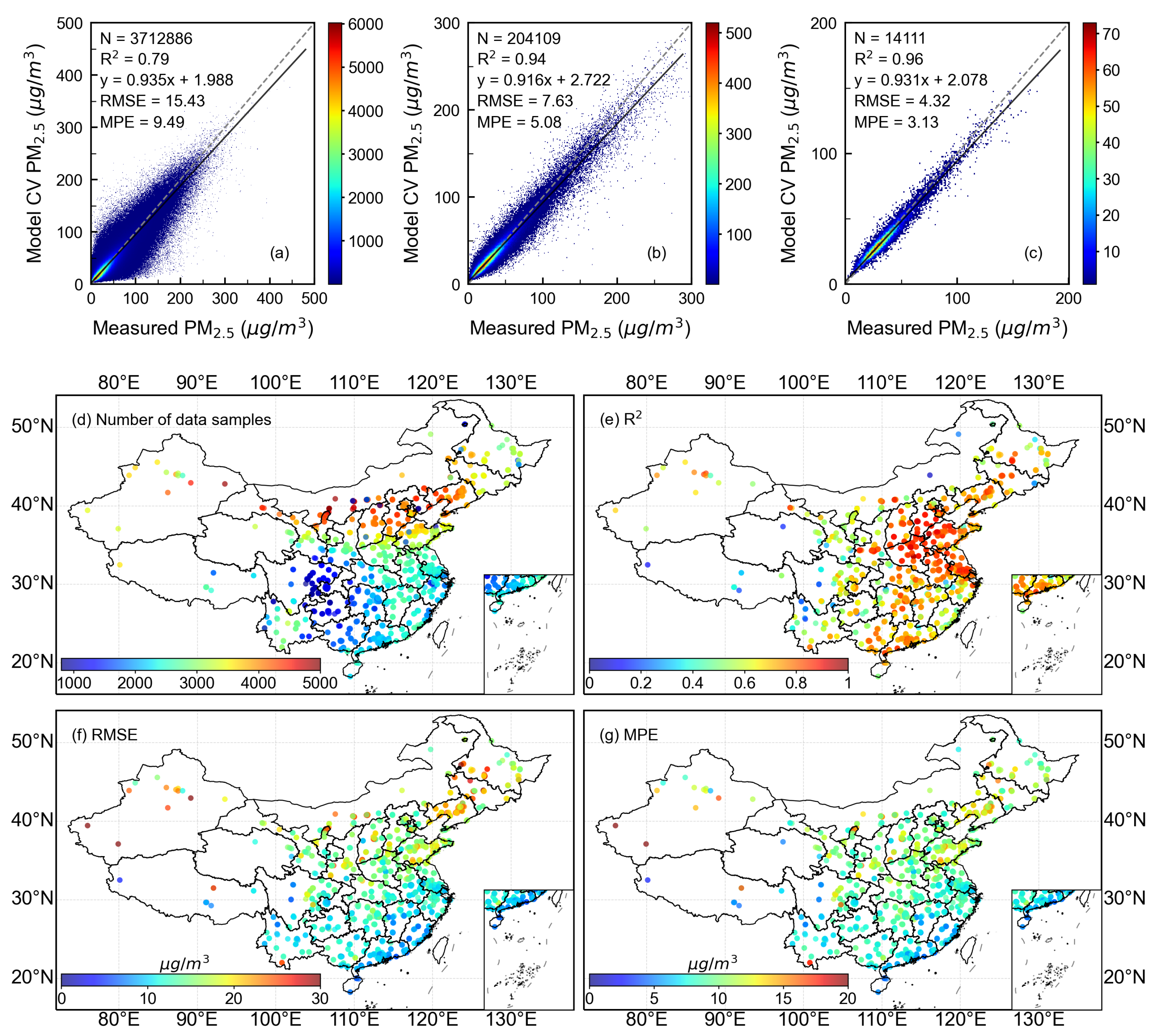
3.1. Cross-Validation Results

The model CV results of the neural network proposed in this study for different time scales are shown in Figure 2a–c. The model CV estimated PM_2.5 concentrations and those measured by ground-based monitoring sites are highly correlated with relatively low prediction errors for hourly, daily and monthly time scales, respectively. The regression lines are very close to the 1:1 line, with slopes nearly equal to one and intercept close to zero. They all suggest that the model does not suffer from substantial overfitting problems and has good performance in accurately estimating PM_2.5 concentrations from the used infrared brightness temperature data and meteorological variables. This is mainly attributed to the massive data samples to better represent data distributions, strong feature representations and nonlinear fitting capabilities of the neural network.

Quantitative results of the model CV for different time scales, which indicates the variability of model estimation for different time scales, are given in

Table 4. Model cross-validation results using the neural network proposed in this study for different time scales.

Time Scale	N	R2	RMSE	MPE	Estimated PM2.5 (Mean ± Std)	Observed PM2.5 (Mean ± Std)
hourly	3,712,886	0.79	15.43	9.49	38.71 ± 31.68	39.27 ± 33.63
daily	204,109	0.94	7.63	5.08	38.44 ± 27.48	38.99 ± 29.91
monthly	14,111	0.96	4.32	3.13	37.41 ± 18.76	37.94 ± 20.11
spring	1347	0.86	3.40	2.53	31.28 ± 7.57	31.87 ± 8.87
summer	1344	0.84	2.88	2.20	23.09 ± 5.56	23.11 ± 6.90
autumn	1363	0.90	3.60	2.71	36.54 ± 9.93	36.88 ± 11.13
winter	1364	0.94	5.06	3.70	53.32 ± 18.69	54.30 ± 20.37

Spring: 202003, 202004, 202005; Summer: 202006, 201907, 201908; Autumn: 201909, 201910, 201911; Winter: 201912, 202001, 202002.

. For hourly estimation, it has relatively high prediction errors because the hourly data samples account for the largest spatiotemporal variability. As for daily and monthly averaged results, the model has a good estimation performance, with R² values of 0.94 and 0.96, respectively. For seasonal results, the model has best performance in winter and the worst in summer. That is because the PM_2.5 concentrations in winter are generally higher than those in summer, and therefore have a higher dynamic range, which can be found in the last two columns in Table 4. In terms of the mean and standard deviation values, the model-estimated PM_2.5 concentrations agree well with the ground-based measurements, with the highest difference ≤1 $\mathsf{\mu }\mathrm{g}·{\mathrm{m}}^{-3}$ and ≤2.5 $\mathsf{\mu }\mathrm{g}·{\mathrm{m}}^{-3}$ for mean and standard deviation, respectively.

In order to investigate the estimation accuracy of the model at different hours of the day,

Table 5. Hourly CV results of the model using the neural network proposed in this study at daily and monthly time scales.

Time (Local)	Daily				Monthly				Time (Local)	Daily				Monthly
	N	R2	RMSE	MPE	N	R2	RMSE	MPE		N	R2	RMSE	MPE	N	R2	RMSE	MPE
0:00	166,377	0.81	15.47	9.53	12,368	0.92	6.55	4.63	12:00	152,564	0.80	14.54	8.91	11,728	0.91	6.20	4.30
1:00	166,577	0.82	15.08	9.38	12,330	0.93	6.36	4.53	13:00	141,850	0.82	13.17	8.16	11,249	0.92	5.67	3.97
2:00	166,300	0.82	14.81	9.22	12,313	0.93	6.17	4.46	14:00	140,156	0.83	12.35	7.69	10,994	0.92	5.04	3.64
3:00	163,446	0.82	15.06	9.28	12,194	0.93	6.22	4.50	15:00	140,360	0.81	12.43	7.61	10,768	0.92	5.00	3.60
4:00	158,182	0.81	15.02	9.31	11,843	0.93	6.11	4.45	16:00	140,209	0.79	13.41	8.00	10,647	0.91	5.24	3.71
5:00	155,585	0.80	15.43	9.61	11,907	0.92	6.36	4.67	17:00	143,018	0.75	15.04	8.84	10,893	0.89	6.24	4.21
6:00	150,552	0.77	16.24	10.09	11,414	0.90	6.91	5.00	18:00	145,908	0.76	15.34	9.38	11,157	0.90	6.30	4.46
7:00	147,568	0.75	16.67	10.59	11,223	0.89	7.11	5.17	19:00	153,659	0.78	15.54	9.67	11,848	0.90	6.63	4.71
8:00	155,714	0.73	17.48	10.96	11,755	0.88	7.44	5.37	20:00	155,622	0.79	15.96	9.92	12,031	0.91	7.00	4.93
9:00	159,155	0.74	17.68	11.03	11,938	0.89	7.53	5.34	21:00	159,746	0.79	16.36	10.07	12,195	0.91	7.07	4.96
10:00	161,732	0.76	16.87	10.41	12,105	0.90	7.22	5.07	22:00	164,020	0.79	16.50	10.09	12,381	0.91	7.14	5.00
11:00	158,642	0.79	15.46	9.49	11,916	0.91	6.61	4.61	23:00	165,944	0.80	15.87	9.73	12,454	0.92	6.73	4.76

gives the hourly results of the model CV at daily and monthly time scales. It can be seen from Table 5 that the R² ranges from 0.73 to 0.83, and from 0.88 to 0.93 for daily and monthly time scales, respectively. Likewise, for RMSE and MPE values, the ranges of variation are very small. Moreover, there is no significant difference in the performance of the model during the daytime (6:00∼18:00) and nighttime (18:00∼6:00), with the mean R² value of 0.777 and 0.797 for daily time scale and value of 0.903 and 0.916 for monthly time scale, respectively. As for the local time 0:00 and 12:00, which are midnight and midday, all the three statistical indicators are very close. It suggests that the model has no systematic bias and has consistent performance at different hours of the day, which offers a way for real-time PM_2.5 monitoring and investigation of the diurnal cycle of PM_2.5. Moreover, the results in Table 4 and Table 5 show that the model has good predictive capability at different timescales.

Figure 2d–g show the spatial distribution of the number of data samples and cross-validation results of R², RMSE and MPE at each site. From Figure 2d, it can be seen that the ground-based monitoring sites in southeastern China are dense, while the sites in northeastern China, especially in the western region, are relatively sparse. The number of data samples in southwestern China, especially in the Sichuan Basin, is relatively small due to frequent cloud cover. From Figure 2e–g, we can see the spatial distribution of estimation accuracy of the model. The R² values of most monitoring sites are greater than 0.7, especially in the North China Plain, where the R² values are generally ≥0.9. This is mainly attributed to large number of data samples and high dynamic range of PM_2.5 concentrations in that region. For some sites in Tibetan region, they usually have relatively low R² values but low RMSE and MPE values which can be seen from Figure 2f,g, because the PM_2.5 concentrations in these places are usually low. Some sites in Northwest China, despite the sparse distribution of sites, still have relatively high R² values. The RMSE and MPE have similar spatial distribution pattern with most of sites RMSE ≤ 20 $\mathsf{\mu }\mathrm{g}·{\mathrm{m}}^{-3}$ and MPE ≤ 13 $\mathsf{\mu }\mathrm{g}·{\mathrm{m}}^{-3}$. The estimation errors in northern China are relatively large because of generally high PM_2.5 concentrations due to pollutant emissions of intensive human activities. The spatial distribution of the results illustrate that our model is robust to the large spatiotemporal heterogeneities and have a good performance over mainland China.

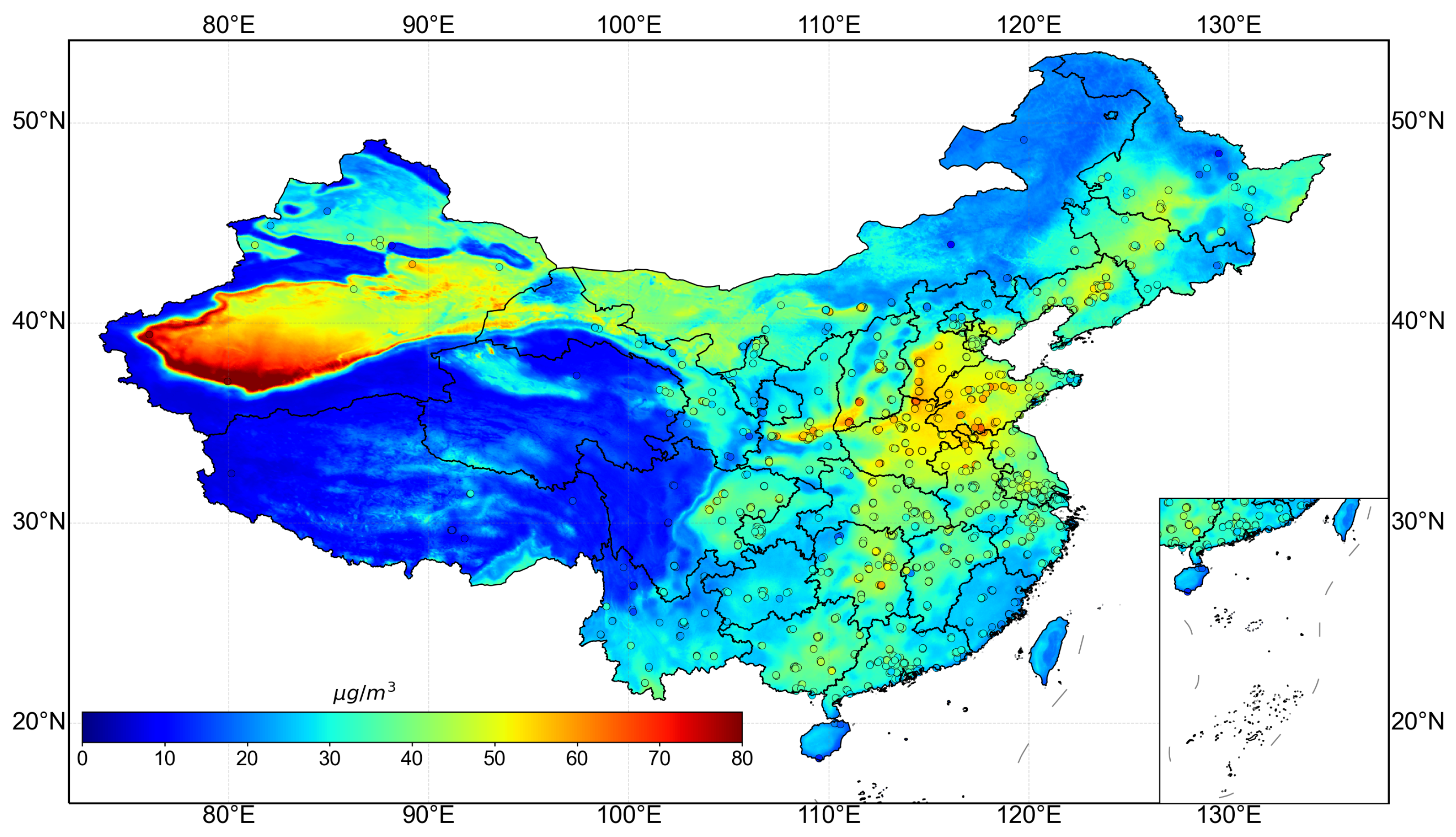
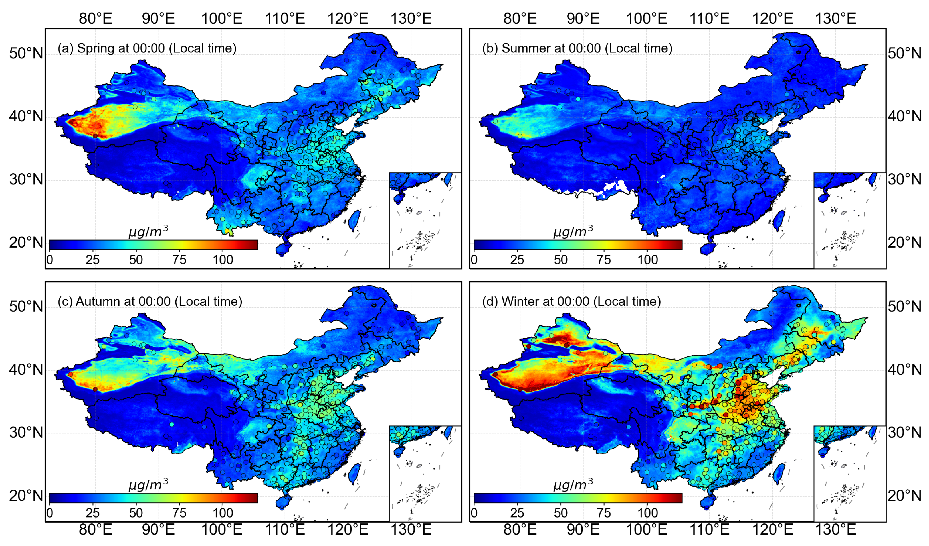
3.2. Spatiotemporal Distribution of Model-Estimated Results in China

Spatial distribution of annually averaged model-estimated PM_2.5 concentrations over China during the study period is shown in Figure 3, and the monthly distribution across China during the study period can be seen from Figure 4. From the annual PM_2.5 concentration map (Figure 3), it can be seen that high PM_2.5 areas are mainly located in densely populated urban areas and desert areas with frequent dust storms. The annual PM_2.5 concentrations in these areas are greater than 35 $\mathsf{\mu }\mathrm{g}·{\mathrm{m}}^{-3}$, which exceed the acceptable level of fine particulate matter pollution. There are obvious seasonal variations, as can be seen from Figure 4. Summer experiences the lowest average PM_2.5 concentration, which is mainly due to more precipitation and lower atmospheric stability in this season. The spatial pattern of PM_2.5 concentrations in autumn are generally similar to those in spring, but slightly higher. Winter experiences the highest pollution level, with many hot spots in the North China Plain, the Northeast Region, and the Taklimakan Desert and Gurbantonggut Desert in the Northwest Region. This is mainly because of intensive human activities, like coal burning for heating in winter, and atmospheric conditions that are limited to the diffusion of pollutants. For any time scales (i.e., monthly and annual), the model estimated PM_2.5 concentrations all have good spatial continuity. In addition, the dots in the figures, which are ground-based measurements during the same period, agree well with the model-estimated values.

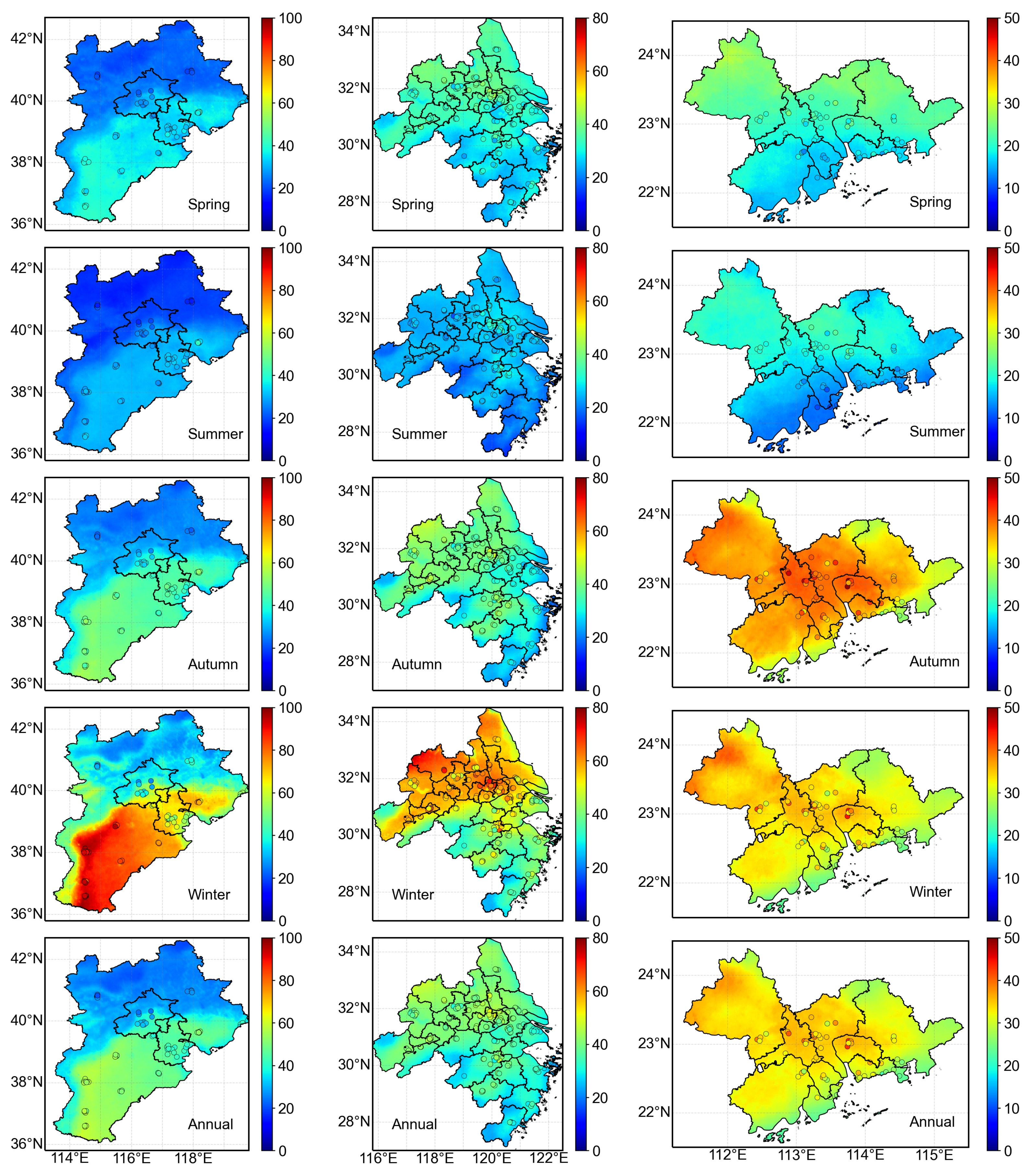
3.3. Results of Typical Regions in China

The Beijing–Tianjin–Hebei region (BTH), Yangtze River Delta region (YRD), and Pearl River Delta region (PRD) are three heavily polluted regions in China with frequent and periodical pollution. Figure 5 gives the spatial distributions of seasonally and annually averaged model-estimated PM_2.5 concentrations over these regions. Overall, the PM_2.5 concentrations in these regions revealed a trend of being higher in autumn and winter and lower in spring and summer. As for BTH, it has the highest PM_2.5 concentrations, especially for the southeastern area with heavy industries. In contrast, the northern mountainous areas have relatively low levels of pollution throughout the year due to restrictions on industrial development. In the case of YRD, the northern areas experience high PM_2.5 concentrations because of dense population and industrial activities, but lower concentrations in the southern hills less influenced by human activities. Compared to BTH and YRD, the pollution level of PRD is lower. Its main pollution comes from human industrial activities and automobile exhausts. Differently from BTH and YRD, people do not need to burn coal for heating in winter, and the average PM_2.5 concentrations are slightly lower than those in autumn, which may be due to the impact of COVID-19 that made human activities significantly reduced in that period. In general, the pollution in these three regions mainly comes from intensive human activities, and is also affected by seasonal climatic conditions that are extremely important for the transmission and diffusion of PM_2.5. By comparison with the ground-based measurements (dots in the figure), it indicates that the model-estimated values are in good agreement with the ground-based measurements, and are also similar to other related studies [1,20,21,34].

3.4. Nighttime Results across China

Besides the hourly results in Table 5 that quantitatively show that our model has consistent performance during daytime and nighttime, in order to further illustrate the model performance in nighttime, Figure 6 gives the seasonally averaged model-estimated PM_2.5 concentrations at midnight (00:00, local time) over China. The dots in the figures are the ground-based measured PM_2.5 concentrations, which are a good demonstration of the accuracy of the model estimations. In general, the PM_2.5 concentrations in the nighttime are higher than those in the daytime, mainly because it is easier to form a temperature inversion layer at night, and the air convection is weakened, which hinders the diffusion of pollutants. Another important reason is that many factories secretly discharge pollutants illegally at night to evade supervision. This also demonstrates the practical significance of this method for environmental monitoring of illegal pollution discharge at night.

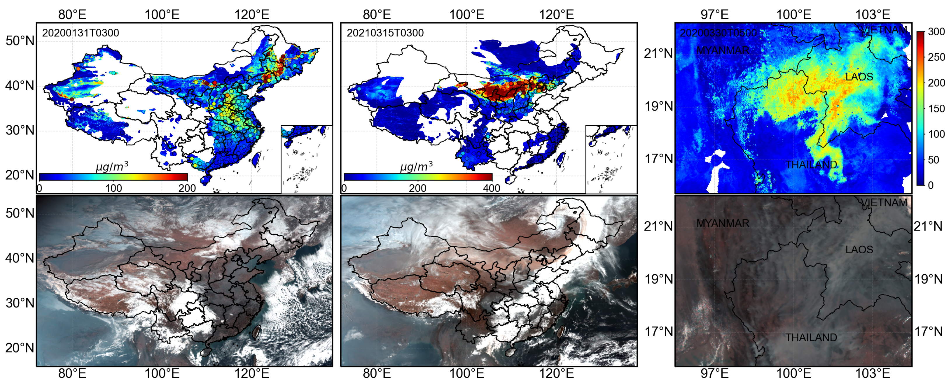
3.5. Typical Test Cases

In order to more intuitively demonstrate the effectiveness of our model, three kinds of environmental pollution incidents, namely heavy air pollution cases, dust storms and fire smoke events, are examined. The first column of Figure 7 shows the case of heavy air pollution. From the corresponding true color image, it can be seen that there is a heavy pollution in the North China Plain. The model-estimated PM_2.5 concentrations can capture the pattern well, and these are consistent with the ground-based measurements. The second column of Figure 7 presents a dust storm event occurred in China in 2021. Affected by the Mongolian cyclone and strong cold air winds, a large-scale of sandstorms, blowing sand and floating dust occurred from central and western Inner Mongolia to northwestern Hebei on 14 March 2021 (local time). From the true color image, we can clearly see the sandstorm. Parts of the dust areas are covered or mixed with clouds. The model-estimated PM_2.5 concentrations show extremely high values in dusty areas. The third column of Figure 7 shows a big forest fire in Southeast Asia. Fires often emit smoke, and this can cause air quality issues, and the distribution pattern is also consistent with that of the model-estimated PM_2.5. From the PM_2.5 concentration maps estimated by the model, and the corresponding true color images of the three kinds of environmental pollution incidents, the accuracy of the estimated PM_2.5 concentrations can be qualitatively and quantitatively verified. It suggests that the model has a robust performance, and is still suitable for extreme weather conditions.

3.6. Comparison with Other Methods

Different from most of other methods that estimate PM_2.5 concentrations through satellite AOD, TOAR or nighttime light imagery, this study develops a deep-learning-based model to estimate hourly PM_2.5 concentration from geostationary satellite infrared bands data, in both daytime and nighttime.

Table 6. Summary of satellite-based PM_2.5 estimation methods applied to China.

Model	R2	MSE	Data	Temporal Resolution	Spatial Resolution	Study Period
Geographically weighted regression [16]	0.64	32.98	AOD	daytime, daily	10 km	2000–2013
Timely structure adaptive modeling [57]	0.80	22.75	AOD	daytime, daily	10 km	2013–2014
Generalized regression neural network [58]	0.67	20.93	AOD	daytime, daily	3 km	2013–2014
Geographically weighted regression [59]	0.79	18.6	AOD	daytime, daily	3 km	2014
Deep belief network [29]	0.88	13.03	AOD	daytime, daily	3 km	2015
Space-time random forest [27]	0.85	15.57	AOD	daytime, daily	1 km	2016
Random forest [34]	0.86	16.8	TOAR	daytime, hourly	5 km	2016
Efficient gradient boosting decision tree [60]	0.86	16.9	TOAR	daytime, hourly	5 km	2016
Deep neural network(ours)	0.79	15.43	BT	full-time, hourly	2 km	2019–2020

summarizes some satellite-based PM_2.5 estimation methods applied on China; some methods that are only applicable to certain local regions in China are not listed. It should be noted that, due to the various types and spatiotemporal coverages of data used among these methods, it would be unreasonable to directly compare the absolute magnitudes of the statistical indicators. As can be seen from Table 6, although our method does not have the highest R² and lowest RMSE values, our method can have a competitive performance compared to other methods. However, our method not only circumvents the intermediate retrievals of AOD, but also takes advantage of the satellite infrared bands that can operate all day and night to estimate PM_2.5 concentrations. This incomparable advantage offers a way of real-time PM_2.5 monitoring and investigation of the day–night cycle.

It is worth mentioning that more ancillary variables, such as land use parameters, population, elevation, surface fire counts, etc., are beneficial to the performance of PM_2.5 estimation models [1]. These variables are directly linked to emission sources and affect the pollution transport conditions. The aim of this study is to demonstrate the potential of using the geostationary satellite infrared bands data, along with some meteorological parameters, to estimate large-scale and hourly PM_2.5 concentrations during both daytime and nighttime. Our method can achieve a comparable performance even without the inclusion of those variables. Integrating more ancillary variables to further improve predictive performance will be considered in future work.

4. Discussion

In this study, we attempted to estimate the PM_2.5 concentrations by leveraging the absorption characteristics of some PM_2.5-related pollutants in the infrared spectrum. We employed infrared brightness temperature measurements from satellite and several meteorological variables to estimate PM_2.5 concentration directly. Considering the correlation between these meteorological variables and PM_2.5, as well as the relatively weak association between BT and PM_2.5 concentration, it is necessary to evaluate the significance of infrared BT data in estimating PM_2.5 concentration. The model was retrained using the same method, but with either meteorological variables or infrared BT data as the inputs. This led to R² values of 0.54 and 0.51, respectively. Compared to the performance of the model that used all the data as input (R² = 0.79), this indicates that there is indeed some useful information in the satellite’s infrared BT data for effectively estimating surface PM_2.5 concentrations.

The deep-learning-based approach is a data-driven method, and the performance of the model is directly influenced by the quality of the data. In this study, there are many factors that may introduce uncertainties into the model’s estimation. For example, ground-based monitoring sites measure the surface PM_2.5 concentration, while satellite data reflects the column characteristics of the atmosphere. Moreover, the measurements from the sites may not accurately represent the PM_2.5 concentrations within a satellite observation pixel. The sample distribution within the dataset may also affect the model performance. Therefore, it is crucial to ensure dataset balance during the creation process. In fact, samples with PM_2.5 concentrations greater than 150 μg · m⁻³ account for only about 1% of the entire dataset, which may lead to underestimation when the model predicts high values. Other factors, such as mismatches caused by different time and spatial resolutions of the data used, also introduce uncertainties in PM_2.5 estimation.

This study achieves large-scale estimation of PM_2.5 concentrations by relying on satellite data with the ground-based measurements as the ground truth. This approach is particularly valuable for PM_2.5 research conducted in areas lacking ground monitoring sites. However, as described by Reichstein et al. [61], models based on machine learning algorithms are relatively effective and static within the observation time period of the dataset used, but exhibit limitations in extrapolating, particularly in situations with extensive temporal and spatial gaps, which lead to reduced predictive performance of the model. Therefore, utilizing real-time data and implementing regular model updates through life-long learning strategies is an effective means to ensure the generalization performance of the model.

It should be noted that this study only used 10 infrared channels of AHI, and the information contained in these channels is relatively weak for estimating PM_2.5. It is worth considering the use of infrared hyperspectral sounder, such as Cross Track Infrared Sounder (CrIS) and High Spectral Infrared Atmospheric Sounder (HIRAS), which has high spectral resolution and can provide rich atmospheric information and more absorption information of pollutants related to PM_2.5 through thousands of channels. Utilizing these sensors can significantly enhance the ability to retrieve PM_2.5 concentrations. However, their spatial resolution is generally low (14 km at nadir). Therefore, it is meaningful to explore the fusion of the imager instruments with the infrared hyperspectral sounder to further improve the retrieval of PM_2.5 concentrations. This research direction will be pursued in our future work.

5. Conclusions

In this paper, we propose a novel perspective to estimate surface PM_2.5 concentrations from satellite infrared bands data. Given the satellite infrared bands can operate all day and night, and some PM_2.5-related pollutants have absorption characteristics in the infrared spectrum, it is possible to directly estimate PM_2.5 concentrations from satellite infrared bands data. Different from other related AOD-based or TOAR-based methods that can not estimate PM_2.5 concentrations in the nighttime, or some other methods based on nighttime light imagery obtained from the satellite day–night band which have many limitations, this study demonstrates the potential of using the geostationary satellite infrared bands data to estimate large-scale and hourly PM_2.5 concentrations in both daytime and nighttime. A specific network and loss function are designed for accurate estimation. An attempt is made to use Himawari-8 infrared bands data to estimate full-time PM_2.5 concentrations by a deep neural network. Quantitative results show that our model has a good performance in accurate PM_2.5 estimation for different time scales and at different hours of the day. Spatiotemporal distributions of monthly, seasonally and annually averaged model-estimated PM_2.5 over China and heavily polluted regions are analyzed. Results indicate that the spatiotemporal variations in PM_2.5 at all time scales can be well captured by our model, and that the model estimated PM_2.5 concentrations are highly consistent with ground-based measurements. Three kinds of environmental pollution incidents events are examined, which suggests the robust performance of our model in extreme weather conditions.

Compared with most of AOD-based or TOAR-based methods, our method can have a competitive performance. Moreover, our method not only circumvents the intermediate retrievals of AOD, but also enable consecutive estimation of PM_2.5 concentrations all day and night. This incomparable advantage offers a way of real-time PM_2.5 monitoring and has practical significance, such as investigation of the diurnal cycle of PM_2.5 and monitoring of illegal pollution discharges at night.

References

1. Ma, Z.; Hu, X.; Sayer, A.M.; Levy, R.; Zhang, Q.; Xue, Y.; Tong, S.; Bi, J.; Huang, L.; Liu, Y. Satellite-based spatiotemporal trends in PM2.5 concentrations: China, 2004–2013. Environ. Health Perspect. 2016, 124, 184–192. [Google Scholar] [CrossRef] [PubMed]
2. Dey, S.; Purohit, B.; Balyan, P.; Dixit, K.; Bali, K.; Kumar, A.; Imam, F.; Chowdhury, S.; Ganguly, D.; Gargava, P.; et al. A satellite-based high-resolution (1-km) ambient PM2.5 database for India over two decades (2000–2019): Applications for air quality management. Remote Sens. 2020, 12, 3872. [Google Scholar] [CrossRef]
3. Semlali, B.E.B.; El Amrani, C.; Ortiz, G.; Boubeta-Puig, J.; Garcia-de Prado, A. SAT-CEP-monitor: An air quality monitoring software architecture combining complex event processing with satellite remote sensing. Comput. Electr. Eng. 2021, 93, 107257. [Google Scholar] [CrossRef]
4. Wang, J.; Christopher, S.A. Intercomparison between satellite-derived aerosol optical thickness and PM2.5 mass: Implications for air quality studies. Geophys. Res. Lett. 2003, 30, 2095. [Google Scholar] [CrossRef]
5. Koelemeijer, R.; Homan, C.; Matthijsen, J. Comparison of spatial and temporal variations of aerosol optical thickness and particulate matter over Europe. Atmos. Environ. 2006, 40, 5304–5315. [Google Scholar] [CrossRef]
6. Lin, C.; Li, Y.; Yuan, Z.; Lau, A.K.; Li, C.; Fung, J.C. Using satellite remote sensing data to estimate the high-resolution distribution of ground-level PM2.5. Remote Sens. Environ. 2015, 156, 117–128. [Google Scholar] [CrossRef]
7. Zhang, Y.; Li, Z. Remote sensing of atmospheric fine particulate matter (PM2.5) mass concentration near the ground from satellite observation. Remote Sens. Environ. 2015, 160, 252–262. [Google Scholar] [CrossRef]
8. Liu, Y.; Park, R.J.; Jacob, D.J.; Li, Q.; Kilaru, V.; Sarnat, J.A. Mapping annual mean ground-level PM2.5 concentrations using Multiangle Imaging Spectroradiometer aerosol optical thickness over the contiguous United States. J. Geophys. Res. Atmos. 2004, 109. [Google Scholar]
9. van Donkelaar, A.; Martin, R.V.; Spurr, R.J.; Drury, E.; Remer, L.A.; Levy, R.C.; Wang, J. Optimal estimation for global ground-level fine particulate matter concentrations. J. Geophys. Res. Atmos. 2013, 118, 5621–5636. [Google Scholar] [CrossRef]
10. Geng, G.; Zhang, Q.; Martin, R.V.; van Donkelaar, A.; Huo, H.; Che, H.; Lin, J.; He, K. Estimating long-term PM2.5 concentrations in China using satellite-based aerosol optical depth and a chemical transport model. Remote Sens. Environ. 2015, 166, 262–270. [Google Scholar] [CrossRef]
11. Engel-Cox, J.A.; Holloman, C.H.; Coutant, B.W.; Hoff, R.M. Qualitative and quantitative evaluation of MODIS satellite sensor data for regional and urban scale air quality. Atmos. Environ. 2004, 38, 2495–2509. [Google Scholar] [CrossRef]
12. Liu, Y.; Franklin, M.; Kahn, R.; Koutrakis, P. Using aerosol optical thickness to predict ground-level PM2.5 concentrations in the St. Louis area: A comparison between MISR and MODIS. Remote Sens. Environ. 2007, 107, 33–44. [Google Scholar] [CrossRef]
13. Sorek-Hamer, M.; Strawa, A.; Chatfield, R.; Esswein, R.; Cohen, A.; Broday, D. Improved retrieval of PM2.5 from satellite data products using non-linear methods. Environ. Pollut. 2013, 182, 417–423. [Google Scholar] [CrossRef] [PubMed]
14. Liu, Y.; Paciorek, C.J.; Koutrakis, P. Estimating regional spatial and temporal variability of PM2.5 concentrations using satellite data, meteorology, and land use information. Environ. Health Perspect. 2009, 117, 886–892. [Google Scholar] [CrossRef] [PubMed]
15. Hu, X.; Waller, L.A.; Al-Hamdan, M.Z.; Crosson, W.L.; Estes, M.G., Jr.; Estes, S.M.; Quattrochi, D.A.; Sarnat, J.A.; Liu, Y. Estimating ground-level PM2.5 concentrations in the southeastern US using geographically weighted regression. Environ. Res. 2013, 121, 1–10. [Google Scholar] [CrossRef]
16. Ma, Z.; Hu, X.; Huang, L.; Bi, J.; Liu, Y. Estimating ground-level PM2.5 in China using satellite remote sensing. Environ. Sci. Technol. 2014, 48, 7436–7444. [Google Scholar] [CrossRef]
17. Song, W.; Jia, H.; Huang, J.; Zhang, Y. A satellite-based geographically weighted regression model for regional PM2.5 estimation over the Pearl River Delta region in China. Remote Sens. Environ. 2014, 154, 1–7. [Google Scholar] [CrossRef]
18. Lee, H.; Liu, Y.; Coull, B.; Schwartz, J.; Koutrakis, P. A novel calibration approach of MODIS AOD data to predict PM2.5 concentrations. Atmos. Chem. Phys. 2011, 11, 7991–8002. [Google Scholar] [CrossRef]
19. Ma, Z.; Liu, Y.; Zhao, Q.; Liu, M.; Zhou, Y.; Bi, J. Satellite-derived high resolution PM2.5 concentrations in Yangtze River Delta Region of China using improved linear mixed effects model. Atmos. Environ. 2016, 133, 156–164. [Google Scholar] [CrossRef]
20. Guo, Y.; Tang, Q.; Gong, D.Y.; Zhang, Z. Estimating ground-level PM2.5 concentrations in Beijing using a satellite-based geographically and temporally weighted regression model. Remote Sens. Environ. 2017, 198, 140–149. [Google Scholar] [CrossRef]
21. He, Q.; Huang, B. Satellite-based mapping of daily high-resolution ground PM2.5 in China via space-time regression modeling. Remote Sens. Environ. 2018, 206, 72–83. [Google Scholar] [CrossRef]
22. Hu, X.; Waller, L.; Lyapustin, A.; Wang, Y.; Liu, Y. 10-year spatial and temporal trends of PM2.5 concentrations in the southeastern US estimated using high-resolution satellite data. Atmos. Chem. Phys. 2014, 14, 6301–6314. [Google Scholar] [CrossRef] [PubMed]
23. Xiao, Q.; Chang, H.H.; Geng, G.; Liu, Y. An ensemble machine-learning model to predict historical PM2.5 concentrations in China from satellite data. Environ. Sci. Technol. 2018, 52, 13260–13269. [Google Scholar] [CrossRef] [PubMed]
24. Xue, T.; Zheng, Y.; Tong, D.; Zheng, B.; Li, X.; Zhu, T.; Zhang, Q. Spatiotemporal continuous estimates of PM2.5 concentrations in China, 2000–2016: A machine learning method with inputs from satellites, chemical transport model, and ground observations. Environ. Int. 2019, 123, 345–357. [Google Scholar] [CrossRef]
25. Ma, Z.; Liu, R.; Liu, Y.; Bi, J. Effects of air pollution control policies on PM2.5 pollution improvement in China from 2005 to 2017: A satellite-based perspective. Atmos. Chem. Phys. 2019, 19, 6861–6877. [Google Scholar] [CrossRef]
26. Hu, X.; Belle, J.H.; Meng, X.; Wildani, A.; Waller, L.A.; Strickland, M.J.; Liu, Y. Estimating PM2.5 concentrations in the conterminous United States using the random forest approach. Environ. Sci. Technol. 2017, 51, 6936–6944. [Google Scholar] [CrossRef]
27. Wei, J.; Huang, W.; Li, Z.; Xue, W.; Peng, Y.; Sun, L.; Cribb, M. Estimating 1-km-resolution PM2.5 concentrations across China using the space-time random forest approach. Remote Sens. Environ. 2019, 231, 111221. [Google Scholar] [CrossRef]
28. Lei, C.; Xu, X.; Ma, Y.; Jin, S.; Liu, B.; Gong, W. Full Coverage Estimation of the PM Concentration Across China Based on an Adaptive Spatiotemporal Approach. IEEE Trans. Geosci. Remote. Sens. 2022, 60, 1–14. [Google Scholar] [CrossRef]
29. Li, T.; Shen, H.; Yuan, Q.; Zhang, X.; Zhang, L. Estimating ground-level PM2.5 by fusing satellite and station observations: A geo-intelligent deep learning approach. Geophys. Res. Lett. 2017, 44, 11–985. [Google Scholar] [CrossRef]
30. Gupta, P.; Christopher, S.A. Particulate matter air quality assessment using integrated surface, satellite, and meteorological products: 2. A neural network approach. J. Geophys. Res. Atmos. 2009, 114, D011497. [Google Scholar] [CrossRef]
31. Feng, X.; Li, Q.; Zhu, Y.; Hou, J.; Jin, L.; Wang, J. Artificial neural networks forecasting of PM2.5 pollution using air mass trajectory based geographic model and wavelet transformation. Atmos. Environ. 2015, 107, 118–128. [Google Scholar] [CrossRef]
32. Chen, X.; Zhang, Y.; Wang, Y.; Zhang, L.; Yi, Z.; Zhang, H.; Mathiopoulos, P.T. A Spatiotemporal Interpolation Graph Convolutional Network for Estimating PM2.5 Concentrations Based on Urban Functional Zones. IEEE Trans. Geosci. Remote. Sens. 2022, 61, 1–14. [Google Scholar] [CrossRef]
33. Wei, J.; Li, Z.; Sun, L.; Peng, Y.; Zhang, Z.; Li, Z.; Su, T.; Feng, L.; Cai, Z.; Wu, H. Evaluation and uncertainty estimate of next-generation geostationary meteorological Himawari-8/AHI aerosol products. Sci. Total Environ. 2019, 692, 879–891. [Google Scholar] [CrossRef]
34. Liu, J.; Weng, F.; Li, Z. Satellite-based PM2.5 estimation directly from reflectance at the top of the atmosphere using a machine learning algorithm. Atmos. Environ. 2019, 208, 113–122. [Google Scholar] [CrossRef]
35. Xie, Y.; Zhao, B.; Zhang, L.; Luo, R. Spatiotemporal variations of PM2.5 and PM10 concentrations between 31 Chinese cities and their relationships with SO2, NO2, CO and O3. Particuology 2015, 20, 141–149. [Google Scholar] [CrossRef]
36. Mao, F.; Hong, J.; Min, Q.; Gong, W.; Zang, L.; Yin, J. Estimating hourly full-coverage PM2.5 over China based on TOA reflectance data from the Fengyun-4A satellite. Environ. Pollut. 2021, 270, 116119. [Google Scholar] [CrossRef] [PubMed]
37. Tang, D.; Liu, D.; Tang, Y.; Seyler, B.C.; Deng, X.; Zhan, Y. Comparison of GOCI and Himawari-8 aerosol optical depth for deriving full-coverage hourly PM2.5 across the Yangtze River Delta. Atmos. Environ. 2019, 217, 116973. [Google Scholar] [CrossRef]
38. Liu, Y.; Li, C.; Liu, D.; Tang, Y.; Seyler, B.C.; Zhou, Z.; Hu, X.; Yang, F.; Zhan, Y. Deriving hourly full-coverage PM2.5 concentrations across China’s Sichuan Basin by fusing multisource satellite retrievals: A machine-learning approach. Atmos. Environ. 2022, 271, 118930. [Google Scholar] [CrossRef]
39. Wang, J.; Aegerter, C.; Xu, X.; Szykman, J.J. Potential application of VIIRS Day/Night Band for monitoring nighttime surface PM2.5 air quality from space. Atmos. Environ. 2016, 124, 55–63. [Google Scholar] [CrossRef]
40. Zhao, X.; Shi, H.; Yu, H.; Yang, P. Inversion of nighttime PM2.5 mass concentration in Beijing based on the VIIRS day-night band. Atmosphere 2016, 7, 136. [Google Scholar] [CrossRef]
41. Fu, D.; Xia, X.; Duan, M.; Zhang, X.; Li, X.; Wang, J.; Liu, J. Mapping nighttime PM2.5 from VIIRS DNB using a linear mixed-effect model. Atmos. Environ. 2018, 178, 214–222. [Google Scholar] [CrossRef]
42. Li, X.; Zhang, C.; Li, W.; Liu, K. Evaluating the use of DMSP/OLS nighttime light imagery in predicting PM2.5 concentrations in the northeastern United States. Remote Sens. 2017, 9, 620. [Google Scholar] [CrossRef]
43. Ji, G.; Tian, L.; Zhao, J.; Yue, Y.; Wang, Z. Detecting spatiotemporal dynamics of PM2.5 emission data in China using DMSP-OLS nighttime stable light data. J. Clean. Prod. 2019, 209, 363–370. [Google Scholar] [CrossRef]
44. Zhang, G.; Shi, Y.; Xu, M. Evaluation of LJ1-01 nighttime light imagery for estimating monthly PM2.5 concentration: A comparison with NPP-VIIRS nighttime light data. IEEE J. Sel. Top. Appl. Earth Obs. Remote. Sens. 2020, 13, 3618–3632. [Google Scholar] [CrossRef]
45. Wang, Y.; Wang, M.; Huang, B.; Li, S.; Lin, Y. Estimation and analysis of the nighttime PM2.5 concentration based on lj1-01 images: A case study in the pearl river delta urban agglomeration of china. Remote Sens. 2021, 13, 3405. [Google Scholar] [CrossRef]
46. Johnson, T.J.; Sams, R.L.; Sharpe, S.W. The PNNL Quantitative Infrared Database for Gas-Phase Sensing: A Spectral Library for Environmental, Hazmat, and Public Safety Standoff Detection. In Proceedings of the Chemical and Biological Point Sensors for Homeland Defense, International Society for Optics and Photonics, 8 March 2004; Volume 5269, pp. 159–167. Available online: https://www.spiedigitallibrary.org/conference-proceedings-of-spie/5269/1/The-PNNL-quantitative-infrared-database-for-gas-phase-sensing/10.1117/12.515604.short (accessed on 4 October 2023).
47. Gordon, I.; Rothman, L.; Hargreaves, R.; Hashemi, R.; Karlovets, E.; Skinner, F.; Conway, E.; Hill, C.; Kochanov, R.; Tan, Y.; et al. The HITRAN2020 molecular spectroscopic database. J. Quant. Spectrosc. Radiat. Transf. 2022, 277, 107949. [Google Scholar] [CrossRef]
48. Bessho, K.; Date, K.; Hayashi, M.; Ikeda, A.; Imai, T.; Inoue, H.; Kumagai, Y.; Miyakawa, T.; Murata, H.; Ohno, T.; et al. An introduction to Himawari-8/9—Japan’s new-generation geostationary meteorological satellites. J. Meteorol. Soc. Jpn. Ser. II 2016, 94, 151–183. [Google Scholar] [CrossRef]
49. Yamamoto, Y.; Ishikawa, H.; Oku, Y.; Hu, Z. An algorithm for land surface temperature retrieval using three thermal infrared bands of Himawari-8. J. Meteorol. Soc. Jpn. Ser. II 2018, 96B, 59–76. [Google Scholar] [CrossRef]
50. Gupta, P.; Christopher, S.A. Particulate matter air quality assessment using integrated surface, satellite, and meteorological products: Multiple regression approach. J. Geophys. Res. Atmos. 2009, 114, D011496. [Google Scholar] [CrossRef]
51. Liu, Y. New Directions: Satellite driven PM2.5 exposure models to support targeted particle pollution health effects research. Atmos. Environ. 2013, 68, 52–53. [Google Scholar] [CrossRef]
52. Hersbach, H.; Bell, B.; Berrisford, P.; Biavati, G.; Horányi, A.; Muñoz Sabater, J.; Nicolas, J.; Peubey, C.; Radu, R.; Rozum, I.; et al. ERA5 Hourly Data on Single Levels from 1940 to Present. Available online: https://cds.climate.copernicus.eu/cdsapp#!/dataset/10.24381/cds.bd0915c6 (accessed on 4 October 2023).
53. Ioffe, S.; Szegedy, C. Batch normalization: Accelerating deep network training by reducing internal covariate shift. In Proceedings of the International Conference on Machine Learning, PMLR, Lille, France, 7–9 July 2015; pp. 448–456. [Google Scholar]
54. He, K.; Zhang, X.; Ren, S.; Sun, J. Deep residual learning for image recognition. In Proceedings of the IEEE Conference on Computer Vision and Pattern Recognition, Las Vegas, NV, USA, 27–30 June 2016; pp. 770–778. [Google Scholar]
55. Girshick, R. Fast r-cnn. In Proceedings of the IEEE International Conference on Computer Vision, Santiago, Chile, 7–13 December 2015; pp. 1440–1448. [Google Scholar]
56. Rodriguez, J.D.; Perez, A.; Lozano, J.A. Sensitivity analysis of k-fold cross validation in prediction error estimation. IEEE Trans. Pattern Anal. Mach. Intell. 2009, 32, 569–575. [Google Scholar] [CrossRef] [PubMed]
57. Fang, X.; Zou, B.; Liu, X.; Sternberg, T.; Zhai, L. Satellite-based ground PM2.5 estimation using timely structure adaptive modeling. Remote Sens. Environ. 2016, 186, 152–163. [Google Scholar] [CrossRef]
58. Li, T.; Shen, H.; Zeng, C.; Yuan, Q.; Zhang, L. Point-surface fusion of station measurements and satellite observations for mapping PM2.5 distribution in China: Methods and assessment. Atmos. Environ. 2017, 152, 477–489. [Google Scholar] [CrossRef]
59. You, W.; Zang, Z.; Zhang, L.; Li, Y.; Wang, W. Estimating national-scale ground-level PM25 concentration in China using geographically weighted regression based on MODIS and MISR AOD. Environ. Sci. Pollut. Res. 2016, 23, 8327–8338. [Google Scholar] [CrossRef] [PubMed]
60. Yin, J.; Mao, F.; Zang, L.; Chen, J.; Lu, X.; Hong, J. Retrieving PM2.5 with high spatio-temporal coverage by TOA reflectance of Himawari-8. Atmos. Pollut. Res. 2021, 12, 14–20. [Google Scholar] [CrossRef]
61. Reichstein, M.; Camps-Valls, G.; Stevens, B.; Jung, M.; Denzler, J.; Carvalhais, N.; Prabhat, f. Deep learning and process understanding for data-driven Earth system science. Nature 2019, 566, 195–204. [Google Scholar] [CrossRef]
Figure 1. The overall structure of our method for satellite-based PM2.5 estimation from geostationary satellite infrared bands data. In the training and validation phases of the model, point data at the ground-based monitoring sites are used, while in the prediction stage, satellite data covering a large spatial extent is used.
Remotesensing 15 04905 g001
Figure 2. The CV results of the proposed model during the study period. The first row is density scatter plots of the results at (a) hourly, (b) daily and (c) monthly time scales. The second and third rows are spatial distribution plots of (d) number of data samples and cross-validation results of (e) R2, (f) RMSE and (g) MPE at each site over China.
Remotesensing 15 04905 g002
Figure 3. Spatial distribution of annually averaged model-estimated PM2.5 concentrations during the study period over China. The dots in the figure are ground-based measurements.
Remotesensing 15 04905 g003
Figure 4. Spatial distribution of the monthly averaged model-estimated PM2.5 concentrations for all hours of a day during the study period over China. The dots in the figures are ground-based measurements.
Remotesensing 15 04905 g004
Figure 5. Spatial distribution of seasonally and annually averaged model-estimated PM2.5 concentrations over three heavily polluted regions in China. The dots in the figures are ground-based measurements. The left column is BTH region, the middle column is YRD region, and the right column is PRD region.
Remotesensing 15 04905 g005
Figure 6. Spatial distribution of seasonally averaged model-estimated PM2.5 concentrations at midnight (00:00, local time) over China for (a) spring, (b) summer, (c) autumn and (d) winter. The dots in the figures are ground-based measurements.
Remotesensing 15 04905 g006
Figure 7. The model-estimated PM2.5 concentrations (the first row) and the corresponding true color images (the second row) for three kinds of environmental pollution incidents of heavy air pollution, dust storm and fire smoke events (from left to right column). The timestamps of the three events are in the upper left corner.
Remotesensing 15 04905 g007