Article

Assessing Landslide Drivers in Social–Ecological–Technological Systems: The Case of Metropolitan Region of São Paulo, Brazil

by
Mayumi C. M. Hirye
1,
Diógenes Salas Alves
2,
Angelo Salvador Filardo Jr.
3,
Timon McPhearson
4 and
Fabien Wagner
5,*
1
Quapá Lab, Faculty of Architecture and Urbanism, University of São Paulo, Sao Paulo 05508-900, Brazil
2
National Institute for Space Research, Sao Jose dos Campos 12227-010, SP, Brazil
3
Faculty of Architecture and Urbanism, University of São Paulo, Sao Paulo 05508-090, SP, Brazil
4
Urban Systems Lab, The New School, New York, NY 10003, USA
5
Institute of the Environment and Sustainability, University of California, Los Angeles, CA 90095, USA
*
Author to whom correspondence should be addressed.
Remote Sens. 2023, 15(12), 3048; https://doi.org/10.3390/rs15123048
Submission received: 1 April 2023 / Revised: 31 May 2023 / Accepted: 2 June 2023 / Published: 10 June 2023

Abstract

:
Urban landslides are increasing globally, mainly caused by human-induced changes in hillsides. Most of these events have caused low-intensity damages to housing and infrastructure. A total of 2038 locations of landslides in the hydrological year of 2010 were used to model landslides’ occurrence in the metropolitan region of São Paulo—Brazil—using a social–ecological–technological system’s approach, which enables the analysis of urban landslides as the outcome of dynamic socioeconomic and infrastructural conditions alongside climatic and geophysical conditions. A multi-step model approach was used to select the best set of variables related to landslides’ occurrence and assess their importance. The value of AUC of the model was 0.9087, denoting the high level of discrimination achieved. Antecedent rainfall played the most important role, followed by terrain slope. Informal settlements, associated with poor constructive practices and a lack of municipal inspection on civil works and buildings, as well as the number of households, which stands for built density and greater alteration in hillsides, yielded a slightly lower contribution. Other variables showed a marginal contribution. These results reinforce the role of local ordinances aimed at restricting occupation in steeper slopes and public policies to promote adequate housing and constructive practices. Future climate projections to MRSP point to the increase in intense rainfall days, making disasters caused by landslides a major source of risk.

Graphical Abstract

1. Introduction

As points of concentration of people and infrastructure, cities are hotspots of risk when exposed to hazards [1,2]. Moreover, the interactions among urban activities can lead, themselves, to risk situations posed by technological failures, natural disasters, such as urban floods or landslides, or even social activities, such as crime, riots, or land invasion [3]. In a context of increasing interaction between society and environment, risks are becoming systemic [4].
Landslides are common events in cities located in hilly areas. Triggered mainly by rainfall, urban landslides are polycausal phenomena [5]. For example, in the Chinese city of Zhouqu, it has been shown that the storm-triggered landslide that resulted in 1765 casualties in 2010 was also related to a combination of factors such as human activity (deforestation and topsoil erosion) alongside geological conditions and terrain modifications caused by an earthquake [6,7]. In 2017, another landslide following heavy rainfall caused more than 1000 casualties in the Regent neighborhood, city of Freetown (Sierra Leone). Poor conditions of rapid and hazardous urbanization were a pre-scenario to this disaster, while increased erosion potential from the clearance of hillsides’ vegetation and weak emergency response acted to amplify its impacts [8].
Globally, landslide occurrence triggered by human activity is increasing, particularly in relation to housing and infrastructure construction, illegal mining, and hill cutting. This supports the idea that human disturbance may be more detrimental to future landslide incidence than the climate [9]. However, countries are not equal concerning landslide risk, and it has been observed that fatal urban landslides occur primarily in less-developed tropical regions, likely because of loss of vegetation cover and alterations in terrain and drainage patterns demanded by urban development, associated with thick weathering layers characteristic of tropical environments [10].
In this context, Sao Paulo is of primary importance in understanding how landslides occur in tropical cities. The metropolitan region of São Paulo (MRSP) is the most important agglomeration in Brazil, in economical and populational terms, and the fourth biggest urban agglomeration in the world [11], with 21.6 million inhabitants. The original site of MRSP is one of the exceptions to the rugged relief of the Atlantic Plateau, a geological unit which covers the southeast of Brazil, alongside the Atlantic coast. Thus, urban development in this unit is distinguished by the coexistence of hills, discontinuous masses, and blocks of raised plateaus, interspersed by valleys with a transversal profile well marked by the dense network [12].
In MRSP, more than 12,000 geological disaster events were recorded in a period of 20 years (from 1993 to 2013) and the majority of these events caused low-intensity damages to housing and infrastructure [13]. Although landslides causing deaths and major economic losses draw public and government attention, low-intensity landslides must not be underestimated. Associated with an extensive risk, these events are more frequent and result in non-neglectable material losses. Low impacts accumulated over time reflect an ongoing erosion of development assets, such as houses, schools, health facilities, roads, and local infrastructure. They are absorbed mostly by residents, progressively undermining their capacity to recover and subsist [14].
Landslides in Southern Brazil mostly occur during the rainy season [9,15], as landslide time series in MRSP have shown the following: a higher number of landslide events were registered during the rainy season, from mid-December to mid-March (Figure 1), and January is usually the month with higher records. In this time series, 2010 was the year with the most landslide records.
While the temporal incidence of landslides has been previously shown for the urban system of MRSP, we are still lacking an analysis including dynamic socioeconomic and infrastructural conditions alongside climatic and geophysical conditions. Landslides have frequently been investigated via susceptibility analysis, which entails the examination of physical attributes of the environment and triggering events. Additionally, vulnerability analysis has been employed, whereby characteristics of the population residing in disaster-prone regions are considered to assess the risk that they face and/or their resilience.
Several methodologies have been employed to generate susceptibility maps for landslides, encompassing physical modeling (e.g., [16]), heuristic methods (e.g., [17]), statistical techniques, such as logistic regression (e.g., [18]), and hybrid approaches combining geographic information systems (GISs) and statistics (e.g., [19]). Notably, the field of landslide susceptibility assessment has witnessed a surge in the application of artificial intelligence and machine learning algorithms, including random forest, artificial neural networks, and support vector machines (e.g., [20]). Moreover, ensemble learning approaches have gained recognition for achieving enhanced performance compared to individual algorithms [21]. These advanced methodologies contribute to improved accuracy and efficiency in landslide susceptibility mapping.
Vulnerability assessment, in contrast, is reliant on expert knowledge and often employs methodologies such as the analytical hierarchy process (AHP) (e.g., [22]) or composite index approaches. These approaches utilize normalized indicators, which may (e.g., [23]) or may not be weighted (e.g., [24]).
In recent years, there has been growing interest in adopting integrated approaches to address the challenges associated with urban landslides. Arrogante-Funes et al. [25] introduced a heuristic model that integrates susceptibility and vulnerability maps to enhance landslide risk assessment. Ahmed [26] examined the underlying causes of landslide vulnerability in Bangladesh, recognizing landslides as socio-natural hazards requiring comprehensive analysis. Other studies have utilized natural and social variables to calculate urban vulnerability indexes for different hazards, including urban floods [24] and landslides [27].
Cities are, par excellence, transdisciplinary problems. Building on complexity theory and the ecosystem approach, multiple frameworks have been proposed to identify and characterize urban components and their relationships (e.g., [28]), envisioning cities as urban social–ecological systems (SESs) composed of two inter-related (sub)-systems: human, which involves social, economic, and cultural aspects of people and institutions, and natural, represented by ecological elements.
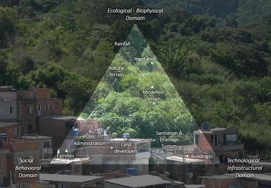
In this paper, we propose to use the socio–ecological–technological system (SETS) approach [29] to correlate dynamic and static social, biophysical, and infrastructural conditions with landslide occurrence in the MRSP. The SETS is intended to look at the cities as complex urban systems, where ecological functions are included in a socio-technological framework that explicitly considers the role of technology and infrastructure within the social–ecological system [30]. The technical–infrastructural subsystem represents the built environment itself, that mediates the relationships between human actions and the environment and can contribute to mitigating or to exacerbating impacts and stressors to this system. From a management point of view, treating infrastructure integrated in a SETS can facilitate the identification and prevention of maladaptive issues that stem from SETS interactions, such as lock-in, as well as offer new perspectives for adaptation strategies that may not traditionally be considered [31,32]. Since its only premises are the interactions between components of these domains, it is flexible enough to accommodate a variate type of analysis from distinctive perspectives to investigate urban systems’ dynamics and complexity [33]. Moreover, this approach can support the urban system characteristics of openness and its multi-scalar nature [34]. The SETS approach has been recently used in assessing urban flood vulnerability [24].
Within this framework, the objectives of this study were (i) to investigate the variables related to landslide occurrence based on the spatial incidence of landslides in MRSP in a logistic regression model, and (ii) to quantify its importance. These were achieved by modeling the landside occurrence in the MRSP, using multi-step regression with a bootstrap strategy. Going beyond a traditional susceptibility analysis, built upon static physical conditions such as lithology or slope degree, we included dynamic socioeconomic and infrastructure conditions inherent to urban systems, as well as ecological variables. Furthermore, considering rainfall alongside this, we were able to assess its importance in relation to other factors within MRSP.

2. MRSP SETS’ Core Components

For the MRSP, we identified the SETS core components that belong to each of the SETS domains: ecological–biophysical, social–behavioral, and technological–infrastructural, based on a literature review. In urban environments, where human-induced changes are prominent, landslide occurrence is the outcome of the relationships between intrinsic characteristics of the biophysical domain with the extension, level, and quality of alteration of slope geometry, surcharge, and water-related processes. These alterations are controlled by actions of dwellers, land developers, and public administration, understood as components of the social–behavioral domain. These actions are materialized in the built environment, which comprises the technological–infrastructural domain and includes buildings, sanitation systems, streets, and drainage systems, which exert influence slope stability.
Most of the literature about landslides is concerned with factors related to the biophysical domain. Rainfall is reported to be the main factor in triggering shallow landslides, i.e., single-slope movements with planar slip surfaces and small lateral dimensions [35,36,37]. There are different ways to measure their effect [38]. In investigations into the relationship between antecedent rainfall and landslides, several authors have considered different periods over which rainfall should be accumulated, ranging from hours to months, e.g., 24 h [39], 3 days [40], 4 days [41], 15 days [42], 31 days [43], or 3 to 4 months [44]. Kirschbaum and Stanley [45] proposed variable thresholds to accumulated rainfall over 7 days to indicate potential landslide activity worldwide. Different periods are due to the type of landslide and regional/local meteorological and physical conditions [46]. In MRSP, thresholds of 60 mm and 80 mm accumulated over 72 h were adopted by Civil Defense to issue a risk alert [47]. Larger periods are considered based on the assumption that the soil water capacity is not achieved by a single precipitation event [37]. Additionally, Ahrendt and Zuquette [48] observed that rainfall temporal distribution is as important as the total amount of rainfall, since cumulative rainfall can lead to complete saturation, while heavy intense rain may not infiltrate but be dissipated by surface runoff.
Common physical variables are those related to terrain characteristics as well as geological and geotechnical characteristics. Besides slope angle, other geometric features were found to influence landslides, such as slope aspect, drainage, surface roughness, topographic indices, elevation, slope length, and curvature [49,50,51]. Varnes [52] presents a compilation of situations regarding the composite materials of slopes, their texture, and structure that account for the geological setting that may be favorable for landslides. The assessment of mass movement susceptibility in municipalities of MRSP considered drainage pattern, slope length, and curvature, alongside landform and substrate characteristics [53]. Rectilinear and concave slopes, with abrupt valley-head slopes, composed of shallow and early-degree pedogenic development over migmatites and granitic gneisses, were identified as being more prone to developing landslides. These highly susceptible slopes were associated with high and low hills and a high density of lineaments/structures.
Vegetation presence can prevent soil erosion [54] and contribute to water infiltration [55] as well as to soil stability, in the sense that plant roots tend to hold soils together [56]. The removal of vegetation cover, as a man-induced process, is often a factor that causes landslides in rural areas as much as in urban areas, as noted by many authors (e.g., [8,57]), particularly in tropical regions.
Intrinsic characteristics and natural processes of the ecological–biophysical domain are altered by the urban occupation of hillsides. This process demands that vegetation is cut and requires the modification of land contours on local and large scales (grading and mass-grading), which is associated with paving, change strength stability of the slope, natural regime of runoff, and infiltration of storm water. Moreover, the introduction of new surface and subsurface water sources associated with irrigation or leaky water from utilities, and the deposition of inadequate material (such as garbage or construction waste) in fills, alter the geotechnical behavior of the natural terrain.
Inadequate building techniques and insufficient design practices employed by families and land developers as well as poor municipal ordinances and weak inspection are unfavorable factors. These are overlapping factors in illegal settlements, which are called favelas (squatters or slums), when families promote the invasion of public or private areas. A different type of illegal settlement is when there is a land developer who promotes the allotment and sells plots, but fails to obtain the legal requirements to approve it. In both cases, there is not a previous design for the land development that could set an appropriate use of terrain, enhancing safety. Sanitary systems are commonly absent. In this paper, these areas are referred to as informal settlements.
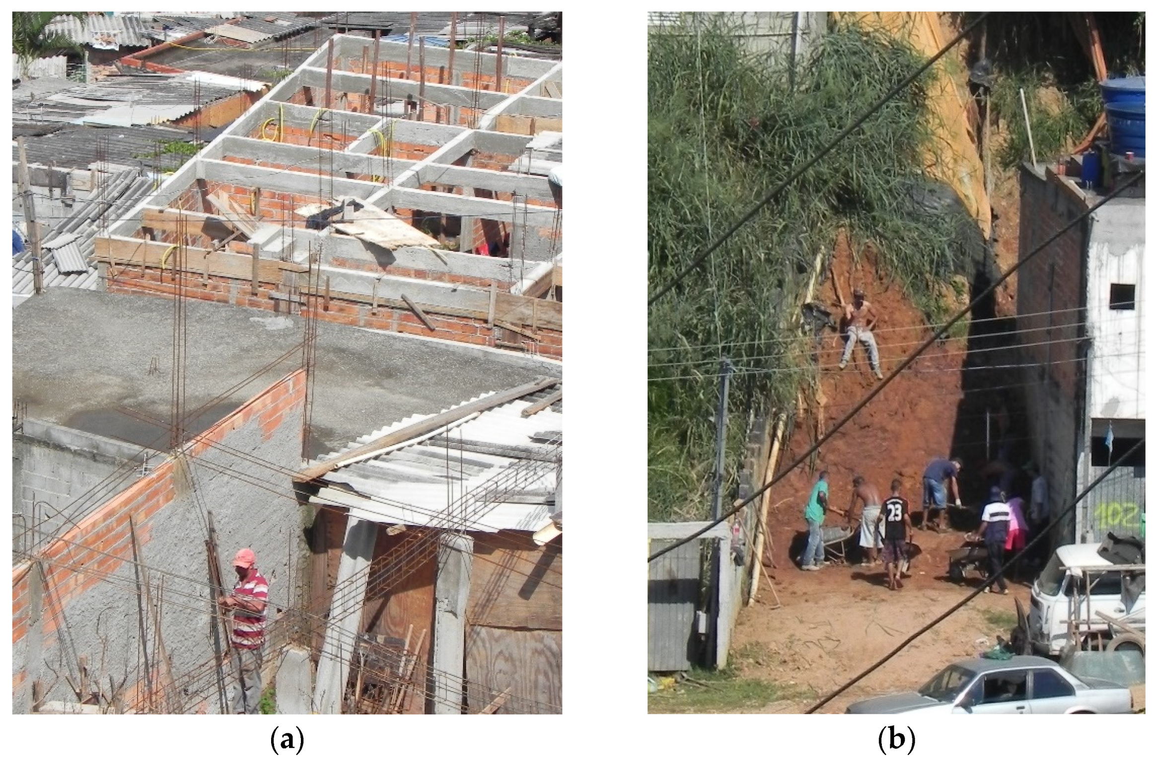
A usual technique observed in favelas is cut-and-fill, e.g., soil removal from the rear of the site and its deposit at the front of the lot, creating a flat area, filled with unconsolidated material extremely susceptible to collapsing [49]. As this is carried out without engineering or any calculation, frequently, the angle at which the headwall is excavated is defined by pursuing the maximization of a flat terrain area, which increases slopes’ susceptibility and damage if a failure occurs. Leaving cuts and fills exposed is a practice commonly observed, favoring soil erosion and destabilization. In some cases, an ordinary plastic protective cover is used to prevent storm water infiltration, resulting in temporary protection. Ref. [58] found similar cut-and-fill practices in the MRSP, also observing fills made using heterogeneous materials (organic debris, plastics, debris, wood, plant remains—trees, branches, leaves, etc.). These technogenic deposits are more instable when compared to cuts, but they may represent a minor risk because in general they are small-sized fills and mobilize less of a volume of heterogeneous materials when a landslide occurs [59]. The illegal settlement situation implicates that civil work and building public inspection that could enhance the safety in these areas are not carried out.
A low income level and limited formal education are components of families’ vulnerability [60]. These characteristics are resources to cope with disaster events. They may also be related to the families’ capacity to build more secure houses. Families with a low income level would have less economic resources to execute adequate grading in their plots and buildings or to contract professional help. A low educational level could be related to less capabilities in building houses via self-aided processes (Figure 2).
The lack of infrastructure systems or their inappropriate design or operation are clearly related to slope security [43,45,49,59,61]. When sewage collection is not universal, solutions such as septic tanks are a possible source of water infiltration, as well as the direct disposal of wastewater [62]. Leakages in sanitary systems are also a source of water infiltration. An absence of storm water drainage elements, including paved streets, accelerates slope erosion and contributes to water saturation and soil surcharge.
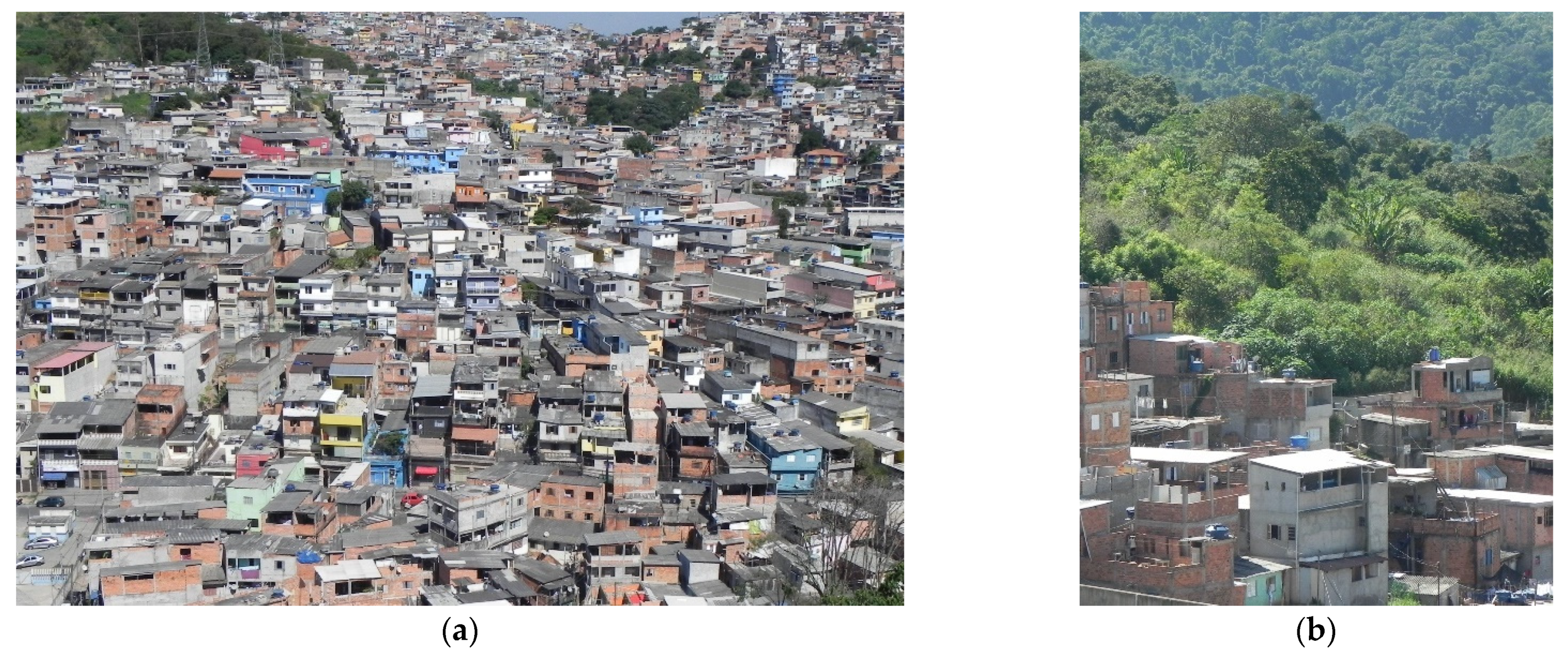
A high density of households, as a concentration of human interventions, has also been related to slope instability, as much as the settlement consolidation level, in the sense that its surfaces tend to become more impervious [36,55,61] and have less vegetation cover (Figure 3).
Smyth and Royle [49] observed that when favelas become more consolidated, materials used in the first dwellings are substituted by more permanent and heavier building materials, implicating an increased load on the terrain. This characteristic is common not only in illegal settlements but also in low-income neighborhoods, in combination with unpaved streets and poor sanitary system conditions [49,55].

3. Materials and Methods

3.1. Study Area

This study was undertaken in the metropolitan region of São Paulo (MRSP), which comprises 39 municipalities and covers an area of almost 80 km2.
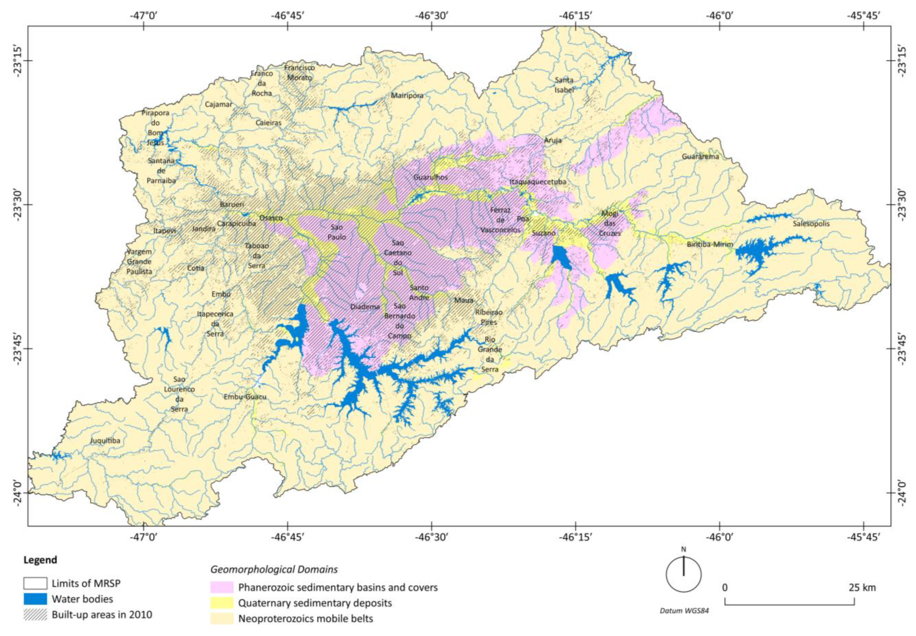
Urban development in MRSP municipalities took place in the flatter areas, formed by phanerozoic sediments, with soft hills and platforms, and by the extensive fluvial plains of the Tietê and Pinheiros rivers, formed by quaternary sedimentary deposits. However, from the second half of the XXth century, the expansion in the pioneer settlement consumed favorable areas and began to advance to the hillsides of the Neoproterozoic mobile belts, formed over a crystalline basement of metamorphic and igneous rocks [63,64] (Figure 4).
MRSP has a humid subtropical climate, with a dry–cool winter and a wet–warm summer (Cwa in Köppen’s classification). The climate is naturally controlled by relief, altitude (ranging from 600 m to 1000 m above sea level), and the short distance to the Atlantic Ocean (about 30 km) [65,66]. The mean annual rainfall is 1400 mm and it is unevenly distributed across the year and in the territory [67]. During the summer season (December, January, and February), rainfall reaches 1100 mm/year, while during the winter season (June, July, and August) it reaches 400 mm/year. Spatially, a strong variation in rainfall in the SE–NW direction can be observed. Long-duration rainfall is associated with cold fronts and it is spatially comprehensive, while lines of instability and the local movement of air, as well as summer storms, result in short-duration rainfall [68].

3.2. Independent Variables

Based on SETS components related to landslides and their relationships described in Section 2, we evaluated the available data on MRSP and selected the independent variables that represent correlated factors with model landslide occurrence (Table 1). Regarding the ecological–biophysical domain, we selected antecedent rainfall, terrain slope and aspect, and mass movement susceptibility, which account for geological, geomorphological, and hydrological–pedological conditions of natural terrain, and percentage of vegetation. Social–behavioral and technological–infrastructural variables were derived from the demographic censuses, carried out every 10 years in Brazil. These data enabled us to characterize, on the one hand, the practices of the families, expressed by their income and educational level, and families’, land developers’, and public administration’s practices associated with the settlement condition (whether informal or not). On the other hand, we characterized the technological–infrastructural domain, selecting sewage system coverage, storm water system conditions (expressed by the existence of street pavements, grating, and curbs), and building density (expressed by the number of households). To account for the settlement consolidation level, we included variables of the difference in vegetation cover, number of households and income, and whether the settlement condition had changed. A framework with SETS domains, components, and variables related to landslide occurrence is presented in Table 1.

3.2.1. Landslide Inventory

Coordinates and dates of landslides were obtained from the Georeferenced Inventory of Geodynamic Events, published by the Geological Institute of São Paulo State (IG) [13]. This database comprises geological, hydrological, and meteorological disaster events registered from 1993 to 2013, in all municipalities of MRSP, except for São Paulo. Event information was gathered from (i) public and private organizations, including state and municipal civil defense agencies, state and federal road operators, and concessionaires; (ii) news published in print and electronic media; and (iii) high-resolution remote sensing data. All registers were classified according to a level of confidence concerning the date and the address of the event, based on the original information available for each event [13]. Since 1993, a total of 30,685 events have been registered. Among them, 12,311 (40.12%) were classified as geological events, comprising the following: debris flows, rock- or landslides, erosion, erosion of the riverbanks, rock fall, soil subsidence and collapse, and mass movement. These events were mostly shallow landslides, that is, rotational or translational slides of engineering soils with small dimensions; a few of them, however, were rockslides [52].
After a consistency check, the following were excluded from the database: (i) events classified with a low level of location accuracy or an estimated/non-informed date; (ii) duplicated registers with the same coordinates and same date or with less than 5 days of difference; (iii) registers with an indication of an inexistent event recorded from field verification; and (iv) registers located out of MRSP’s municipal boundaries. Finally, we kept registers from 2001 to 2013, since until 2001, registers were not complete because data were collected only during the rainy season. This exclusion resulted in a database of 8066 landslides’ locations, and from which a total of 2038 were in the 2010 hydrological year (from October 2009 to September 2010) and were used to model the landslide occurrence. According to the inventory, these landslides caused a total of 18 fatalities, thereby characterizing them as predominantly low-intensity landslides.

3.2.2. Rainfall Data

Daily rainfall (mm) was obtained from the Climate Hazards Group InfraRed Precipitation with Station Data (CHIRPS)—version 2.0 [69]—available on Google Earth Engine. CHIRPS incorporates satellite imagery with in situ station data to create gridded rainfall time series at a resolution of 0.05 arc degrees. In MRSP, 35 in situ stations were incorporated to infrared cold cloud duration (CCD) observations calibrated using the Tropical Rainfall Measuring Mission Multi-Satellite Precipitation Analysis version 7 (TMPA 3B42 v7) to estimate daily rainfall.

3.2.3. Elevation-Related Variables

Variables related to terrain—slope and aspect—were based on a digital elevation model (DEM), with 10 m spatial resolution. DEM was derived from the digital planimetric and topographic map of MRSP, with 25 m contours [65] and a spatial scale compatible to 1:25,000, using a triangulated irregular network (TIN) calculated based on contour lines, measured points, and a river network. Terrain slope (in degrees) was obtained using the first-order derivative estimation, as proposed by [70]. Aspect is the direction that a slope faces, measured from 0° (north) to 360°, in a clockwise direction. This variable was categorized, adopting 4 directions, with each one encompassing 90°, and centered in 0° for north, 90° for east, 180° for south, and 270° for west, and was related to flat areas (where aspect was null).

3.2.4. Physical Mass Movement Susceptibility

Mass movement susceptibility classification was performed based on geological, geomorphological, and hydrological–pedological conditions [53], by the Geological Survey of Brazil (“Companhia de Pesquisa de Recursos Minerais”—CPRM), for all municipalities in MRSP, except Vargem Grande Paulista, Pirapora do Bom Jesus, Juquitiba, and São Lourenço da Serra. Maps are available as digital vector data, compatible to 1:25,000. Zones were classified into high, medium, or low susceptibility, according to the predominant characteristics in each municipality.

3.2.5. Land Cover Data

Land cover classes of vegetation, built up areas, bare soil, and water were mapped from Landsat TM, at a spatial resolution of 30 m, using Landsat Collection Tier 1, processed and made available by the U.S. Geological Survey (USGS). A supervised classification approach based on the support vector machine (SVM) was applied to visible and infrared bands (red, green, blue, and NIR bands), the normalized difference vegetation index (NDVI), the mean NDVI computed for the summer season, and the mean NDVI of the winter season. The classification model was built with 677 random samples visually classified on orthophotos of the year 2010, and divided into two equally sized groups for training and validation. An overall accuracy of 89.8% (confidence intervals of [0.873, 0.920]) and kappa index of 0.844 were obtained from the confusion matrix. This model was applied to 1992 images and the land cover classes were remapped to obtain a vegetation cover map of 1992 and 2010. The year 1992 was chosen to be a reference for the 1991 census data. Additionally, the vegetation change between 1992 and 2010 was computed based on the vegetation cover maps.

3.2.6. Demographic Census Data

In this paper, the demographic census data from the Brazilian Institute of Geography and Statistics (“Instituto Brasileiro de Geografia e Estatística”—IBGE) and georeferenced census tracts, processed and made available by the Center for Metropolitan Studies (“Centro de Estudos da Metrópole”—CEM), were used. The selected variables from the census data were as follows: number of households, to account for built density, and percentage of households without sewerage, on unpaved streets, on streets without storm sewers (curb and grating), and on streets with open sewage, to characterize the built environment.
To characterize families, variables of average income of the individual responsible for the household (household’s head) and percentage of literate household heads were selected to account for their levels of education. To characterize families’ and land developers’ built practices, as well as the public administration role, the settlement’s condition (regular or subnormal) was used. In the census database, subnormal settlements correspond to favelas and illegal allotments. They are identified as tracts with 51 or more housing units characterized by the absence of title deeds, irregularity of the roadways and the size and shape of plots, and/or lack of essential public services (such as garbage collection, sewage, water and electricity systems, and public lighting) [71,72].
Census data were interpolated into a grid, using dasymetric mapping, following similar approaches for world data [73] and for regional and local data [74,75,76]. Street networks made available by CEM and built-up areas from land cover maps, as previously described, were used as ancillary data to spatially disaggregate the census tracts.

3.3. Database Preparation

To model the occurrence of landslides in the MRSP, the hydrological year of 2010 was selected, since for this period, the most complete datasets of meteorological and census variables are available. Therefore, the period between 1 October 2009 and 30 September 2010 was adopted, contemplating the entire wet period, from October to March, in one year, in accordance with recommendations for susceptibility and hazard mapping [77,78,79].
The geocoding of landslide events reports the street name and the address number where the event occurred, which consequently results in locations systematically along the streets. To estimate where the landslide likely occurred, 30 m was adopted as a mean distance from the center of the street to the interior of the plot to account for this mis-location. All areas within the built-up area in MRSP and outside the 30 m buffers around the landslide location were considered to be areas of non-occurrence of landslides. These areas were divided into a 10 m grid cell, and to each cell center, a point was assigned to create points of non-occurrence of the landslide. A random date was assigned to each of these points.
For each point, antecedent rainfall from 1 to 120 days was computed. In this paper, we selected different periods to be tested, ranging from rainfall in the same date for each point up to the rainfall accumulated over 120 days. The upper boundary was defined based on the period between the beginning of the wet season (October) and the peak of the landslide occurrence (January). Based on the coordinates and dates, we extracted the antecedent rainfall of each point of occurrence and non-occurrence of landslides for all of the periods considered.
Before the extraction of each independent variable’s value related to each location of disaster and non-disaster, all variables were resampled to a grid with a spatial resolution of 10 m. Then, to account for the mis-location of landslide points of occurrence, variables were spatially aggregated using a sliding window of 7 × 7 grid cells in 10 m grids, using an appropriate function. For terrain slope, we used the maximum value; for mass movement susceptibility and subnormal condition of the settlement, we used the modal value; for households, we used the sum of values; and, for vegetation and family’s characteristics (income and literate status), we used the mean value. In the case of vegetation, since it is a binary map (0: non-vegetation, 1: vegetation), the mean value also expresses the percentage of vegetation within the considered distance. From these focal filtered grids, we derived four other variables that accounted for changes in the conditions between 2010 and 1991: vegetation, households, income, and settlement’s condition change.
Landslide inventory and mass movement susceptibility maps did not cover all of the municipalities of MRSP. Therefore, analysis excluded the following municipalities: Biritiba-Mirim, Cajamar, Embú-Guaçu, Embú, Franco da Rocha, Itapevi, Juquitiba, Poá, Pirapora do Bom Jesus, Salesópolis, São Caetano do Sul, São Paulo, São Lourenço da Serra, and Vargem Grande Paulista.
For validation purposes, we split the database into an 80–20% proportion, preserving the balance between categories of the dependent variable (landslide occurrence and non-occurrence).

3.4. Model Development

Modeling was developed in two steps: exploratory analysis and landslide occurrence modeling. Firstly, the association between landslide occurrence and climatic, biophysical, and census’ variables was explored using Student’s t-tests to compare the mean of the quantitative explanatory variables between the two groups: landslide and non-landslide. For the categorical variables, the equality of the proportion between the groups’ landslide and non-landslide was performed using the chi-squared test to test the difference in the distribution within each category of these variables between the two groups. In this step, we made a first selection of the variables, removing variables that were not different between the two groups. Complementing this, appropriate statistical measures were calculated to assess the correlation between all of the continuous and categorical variables.
In the second step, univariable and multi-variable logistic regression models were developed to obtain a quantitative estimation of landslide hazard and the contribution of each factor to its occurrence. A logistic regression model is a widely used approach in the literature related to landslides [18], it is reported to yield lower error rates and the best generalization capabilities [80]. This model has the following form:
g(x) = ln (π(x)/(1 − π(x)) = β0 + βi x
where g ( x ) is the logit, π ( x ) is the probability of the event occurrence given the independent variable’s value (x), and β 0 and β i x are the regression parameters.
Logit is a transformation applied to the probability of an event’s occurrence. It is also known as the odds ratio and it expresses the chance of a landslide event given an increment in any of the independent variables’ value. For continuous variables, eβi corresponds to the chance for an increase of 1 unit in this variable. For categorical variables, eβi will express the chance of landslide occurrence when the independent variable assumes one class in comparison to another class. In logistic regressions, parameters are obtained using maximum likelihood estimation.
Parameters and statistics, as well as their confidence intervals, were estimated using bootstrap as a resampling technique with a probability of 95%. This is recommended to provide stable estimates with low bias [81,82]. All models were run 1000 times with randomly generated sets of samples, each one with 1000 points of landslide occurrence and 1000 points of non-occurrence.

3.5. Model Performance Assessment

The assessment of univariable models was performed based on their significance, using a high level of tolerance (p-value < 0.25) to prevent discarding variables that could add some level of explanation in the multi-variable analysis. Therefore, variables with non-significant parameters in relation to the landslide occurrence calculated were disregarded.
Univariable logistic regression models were also calculated in order to select the best antecedent rainfall period. These models were then compared using a modified version of Cox and Snell’s index adjusted to constrain the index value not to exceed 1 (Equation (2)). This approach is analogous to R2 in an ordinary linear model but adapted for logistic regression. Although it is useful to compare logistic regression models [83], they are not recommended to be used to report final results [84], since this index, along with others such as pseudo-R2, can lead to misinterpretations of the model’s predictive strength in the sense that they yield lower values if compared to values of ordinary least squares R2 obtained under similar conditions [85].
R2n = (1 − (Lo/Lm)2⁄N)/(1 − exp (−Lo/N)
where R2 is likelihood in the chi-squared test, Lo is the likelihood functions for the constant-only model, Lm is likelihood functions for the fitted model, and N is the sample size.
A multi-variate model with all variables selected in the univariable model’s step was fit to enable the selection of significant variables and to assess the main effects from their interaction. All variables yielding a level of significance higher than 95% were retained to a preliminary complete model. The final assessment was to compare this preliminary complete model to others, fitted with a subset of its variables, using the Bayesian information criterion (BIC) [86]. From this final analysis, we selected the model yielding the highest predictive strength and the smallest and most significant set of independent variables.
To assess the predictive information of each of the independent variables, we used an adequacy index, based on the likelihood ratio test [83]. It is expressed as the ratio between the −2 log likelihood ratio statistic for testing the joint significance of a model with a full set of variables and the −2 log likelihood ratio statistic for testing the importance of a model with only one variable. This index estimates the proportion of log likelihood explained by the variable with reference to the log likelihood explained by all variables, which can be understood as the contribution of each variable to the model.
The goodness-of-fit of the final model was evaluated using the area under the receiver operating characteristics curve (AUC). This was performed using the test samples. The AUC ranges from 0 to 1 and values lower than 0.5 suggest that the model yields no discrimination between points of occurrence of landslides and non-occurrence. As a general rule, AUC values from 0.7 to 0.8 suggest acceptable discrimination and from 0.8 to 0.9 suggest excellent discrimination. Values higher than 0.9 suggest outstanding discrimination, although for logistic regression models it is extremely unusual to observe such high values [84].
All analyses were performed using the R-project software (http://www.r-project.org/, accessed on 6 June 2023).

4. Results

Our results encompass the identification of the best way to account for rainfall, the identification of relevant variables to model landslide occurrence and the mathematical expression of this relation, and the analysis of these variables in terms of their contribution to landslide occurrence and the risk associated with an increment in each of these variables.

4.1. Antecedent Rainfall

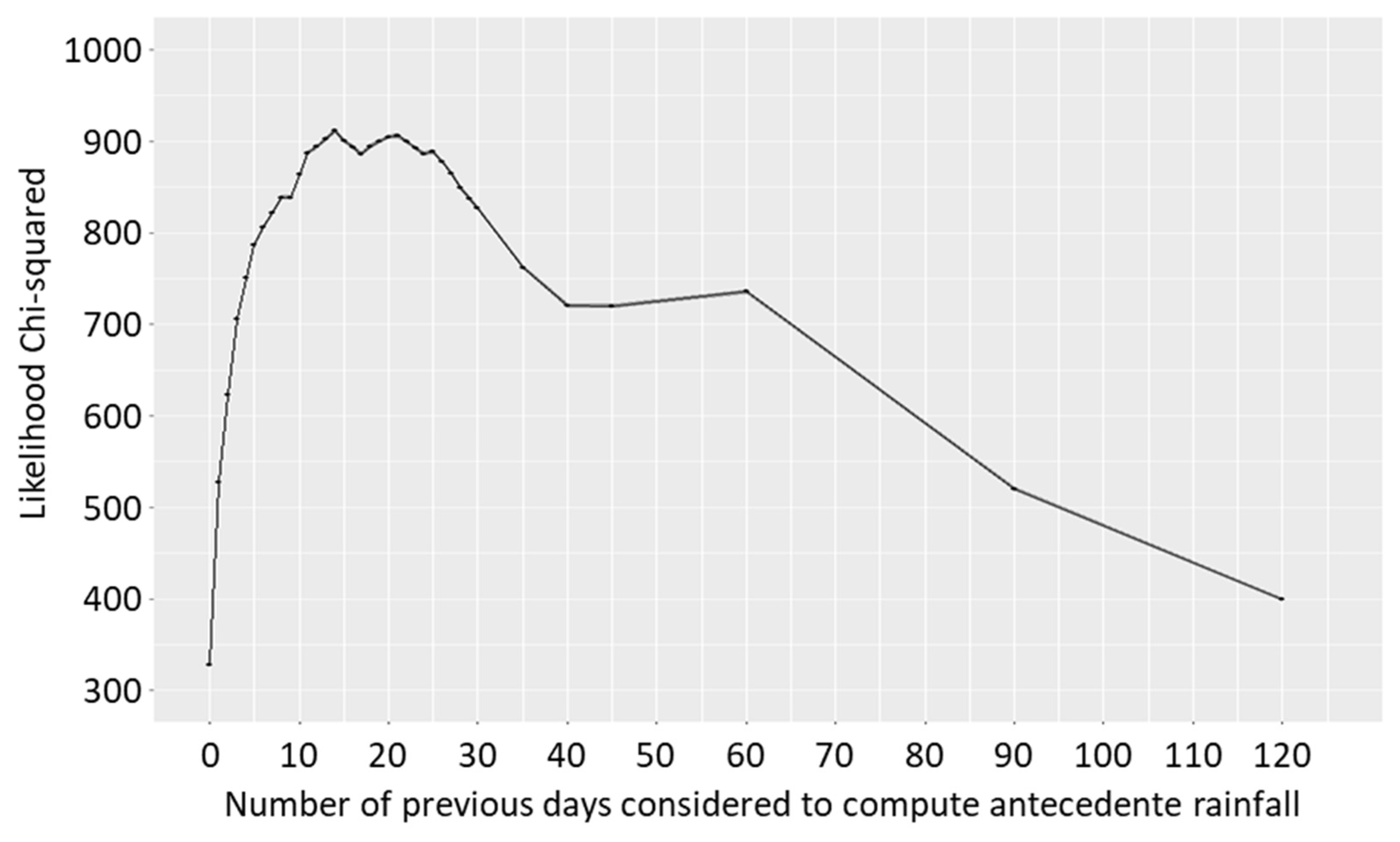
We found that the cumulative precipitation of the 14 previous days was the best way to account for the soil water saturation in MRSP. The importance of cumulative rainfall preceding the occurrence of landslides exhibits clear behavior in the univariable model (Figure 5). Up to 14–20 days, it has rising significance, estimated by the high value of the likelihood chi-squared test. This importance is maximal if computed with the 14 days of previous rainfall and declines sharply with more than 25 days.
This section may be divided by subheadings. It should provide a concise and precise description of the experimental results, their interpretation, as well as the experimental conclusions that can be drawn.

4.2. Landslide occurrence Model

The landslide occurrence model was built after carrying out an exploratory analysis of all variables and an assessment of uni- and multi-variable models. The results of these steps are presented in Appendix A and Appendix B. For the final model, the variables retained were as follows: antecedent rainfall (day and 14 previous days), two biophysical variables (slope and percentage of vegetation), two variables of the social domain (average household head’s income and settlement condition), and three variables characterizing the built environment (households, percentage of households without sewerage, and percentage of households on streets without a storm sewer (curb) in 2010). They are all statistically significant at the 5% significance level and, except for average household head’s income in 2010 and percentage of households without sewerage, they all have a positive relationship with landslide occurrence (Table 2).
The final analysis, performed using BIC criteria, showed that the model fitted with all of the selected variables was better than any other model fitted with subsets of these variables (Table 3).

4.3. Variables’ Contribution

Antecedent rainfall plays the most important role in landslide occurrence: this variable corresponds to 0.70 of the predictive information of all variables combined alone, according to the calculated index of adequacy (Table 4). For terrain slope, this index is 0.20. Settlement conditions and households have similar predictive information proportions, 0.15 and 0.14, respectively. Other variables have smaller contributions, with the index of adequacy below 0.06.

4.4. Landslide Occurrence Risk

Considering only antecedent rainfall, each increment of 10 mm will raise the chance of a landslide by 1.177 times (Table 5). Similarly, increments in terrain slope, percentage of vegetation cover, households, and percentage of households on streets without a storm sewer (curb) will result in a higher chance of landslide occurrence. Increments in the average household head’s income and percentage of households without sewerage, on the contrary, will decrease the chance. Remarkably, landslides in subnormal settlements have 4.634 times more chance of occurring than in a regular settlement.

5. Discussion

An extensive landslide inventory associated with gridded thematic data layers and a bootstrap strategy contributed to a robust statistical result. A theoretical and data-gathering effort was made to model landslides, associating them with biophysical, social, and built environment variables.

5.1. Importance of Ecological–Biophysical Variables in Landslide Occurrence

There is a strong association between landslides and rainfall in MRSP: this variable accounted for 70% of the predictive information of the model. Furthermore, we also found an important contribution of antecedent rainfall, likely representing soil water saturation, in accordance with early observations in Brazil made by [41], followed by the Civil Defense in São Paulo state in establishing the awareness level. The modeling results pointed to a period of 14 days to account for the total antecedent rainfall: for the points of landslide occurrence, this total was, on average, 216 mm, while for points of non-occurrence, it was 83 mm (Table A1, Appendix A). Climate projections for 2070 and 2100 foresee the doubling of the days with intense rain (higher than 10 mm) [67]. Accumulated rainfall in this context will increase and act to saturate the soil in a shorter period, concurring to undermine slope stability and raise landslide risk. Landslide hazards on time scales affected by climate change can be quantitatively characterized via a combination of climate models and precipitation estimates, as recently shown by Kirschbaum et al. [87].
Terrain slope gradient accounts for natural terrain’s most important characteristic related to landslide occurrence. In our model’s results, it accounted for 20% of the model’s predictive information. Other geological, geomorphological, and hydrological–pedological aspects, very often highlighted in the landslide literature (e.g., [54,79]), were treated in this research as areas of mass movement susceptibility. Nevertheless, in urban areas of MRSP, medium- and high-susceptibility classes were found to be correlated with steeper slopes and subnormal settlements. For this reason, the mass movement susceptibility variable was deprecated in fitting the logistic regression model performed in this paper, despite its importance in physical-process-based models of landslides. Slopes and settlement conditions offered greater explanation in landslide occurrence.
Vegetation is of great importance to water infiltration processes and in preventing soil erosion and instability. Nevertheless, its presence was positively related to landslides. This result is contradictory with much research that relates vegetation cut with landslides (e.g., [8,43]). The mean percentage of vegetation was of only 10% at points of non-occurrence of landslides, while at points of landslide occurrence, it was higher, at 22.7% (Table A1, Appendix A). Vegetation cover likely represents an indirect indicator of open spaces and pervious surfaces. We hypothesize that its higher percentage in landslide points denotes areas that have been left unoccupied, often because of severe physical restrictions, surrounded by impervious areas without an adequate surface water drainage system. Thus, these open spaces may become areas of accumulation and infiltration of water, causing the saturation of the soil and its eventual rupture, despite the presence of vegetation, whose roots could contribute to water absorption and soil cohesion.

5.2. Importance of Social–Behavioral Variables in Landslide Occurrence

Previous work has already pointed to the role of unfavorable housing and urbanization conditions in landslide occurrence [88,89,90]. In this paper, these conditions were identified with subnormal settlements, which are associated with illegal allotments and favelas, inadequate practices of cut-and-fills, the creation of technogenic deposits, self-aided building, and lack of inspection, reflecting poor building practices of families and land developers, as well as a weak role of public administration. They accounted for 15% of the predictive information of the landslide occurrence model. The dramatic difference in settlement conditions is expressed by the chance of landslide occurrence being 4.6 times higher in a subnormal settlement than in a regular one. Income posed a minor contribution to landslide occurrence, corresponding to 6% of the model’s predictive information. This may be due to a bias of census data, caused by the declaratory nature of this information. The average monthly household income in the points of landslide was BRL 1828 in 2010 (approximately USD 968 in 2023). An increase of BRL 100 in this income would imply a 0.99 chance of landslide occurrence. This may suggest that landslide occurrence is related to a problem of access to housing, rather than solely a matter of income. This hypothesis is reinforced by the fact that dwellers at points of landslide occurrence have a similar level of income to their neighbors, but different reasons rather than just economic resources made them occupy these areas.
Educational level did not result in being relevant to landslide occurrence, at least in terms of educational level measured by the variable available in the census data—percentage of literate individuals responsible for the household. This variable may not be adequate to measure families’ capabilities to properly build their houses via self-aided processes.

5.3. Importance of Technological–Infrastructural Variables in Landslide Occurrence

The number of households was taken as a representative measure of the number of buildings, characterizing the built environment, and yielded 14% of the predictive information of the landslide occurrence model. Therefore, a high density of buildings, and consequently major slope interventions, correspond to a higher probability of landslide occurrence.
Descriptions of landslide events reported the role of wastewater or storm water disposed directly into the soil. Strong evidence in the literature supports the causal relationship between water infiltration and landslides (e.g., [41]). Hence, variables of the percentage of households without sewerage, without a storm sewer (grating), and on streets with open sewage were expected to have higher values in landslide occurrence points. Surprisingly, for MRSP, the results were the opposite. Our hypothesis is that either sewage and storm water leakages are very often associated with a higher coverage of this infrastructure system, or these results may be related to the fact that in MRSP extensive areas have low coverage of these systems and areas where landslides have occurred are not representative of this situation. Indeed, an average of 26% of the households within the buffer of each point of landslide non-occurrence do not have access to sewerage, while within the buffer of the landslide occurrence points, the average is of 17.8%. This same difference in situations is observed regarding the inexistence of storm sewers (grating) and the presence of open sewage on streets. Regarding the former variable, averages were of 45.8% in areas of non-occurrence and 39.8% in areas of occurrence, while for the latter, averages were of 6% and 4.6%, respectively. These percentages suggest that areas of landslide occurrence are, on average, in a better situation than areas of non-occurrence, and this difference, in the case of the variable related to sewerage, may have yielded a minor contribution (2%) to the predictive information of the model.

5.4. Landslide Occurrence from Social–Ecological–Technological System’s Perspective

The fact that the majority of landslide fatalities occur in cities of less-developed countries points to their intrinsic vulnerability due to the existence of larger areas of precarious settlements [1,56,91]. Moreover, hazardous climatic conditions pose an additional challenge for landslide management and prevention [10]. In the MRSP, both conditions occur: particularly intense rainfall during the summer season, when most of the landslides occur, and precarious settlements exhibiting hazardous conditions. Vulnerability raised from precarious settlements’ existence, on the other hand, is a combination of inadequate and precarious hillside occupation with social vulnerability of a population that have this as the only solution to a housing problem. In both cases, government actors fail in their policies to ensure social and environmental protection.
In this scenario, public administration must take actions not only based on monitoring and warning systems, but mainly in preventing precarious occupation on hillsides. Moreover, a shift in culturally adopted techniques leveraging building practices, both related to buildings and cut-and-fills, would contribute to slope stability and could lead to a positive transformation in hillside occupation patterns in the MRSP.
This study is aligned with recent efforts to assess risks in an integrated framework, bridging the gap between susceptibility and vulnerability analysis [24,25,26,27]. By considering variables within a comprehensive framework, this study identifies the crucial factors that are decisive in addressing landslide risks. Notably, rainfall emerges as the most prominent factor, highlighting the formidable challenges posed by climate change in the study area, considering that future climate projections indicate an increase in the frequency of intense rainfall days [67]. Steep slopes constitute the second significant factor, along with subnormal settlement conditions. In this regard, the public administration indeed has a pivotal role in taking proactive measures to prevent slope occupation, to ensure adequate protection measures, to implement slope stabilization infrastructure, and, in some cases, to relocate families.
This study also incorporates ecological and infrastructural variables that are often overlooked in landslide assessments. In this context, two counterintuitive observations were made: (1) areas without landslide occurrence exhibited a higher prevalence of infrastructure deficiencies, particularly in sewage systems; (2) areas with landslide occurrence showed a higher presence of vegetation. While these findings do not imply a lack of association between these variables and landslides, their relatively minor significant contribution to landslide occurrence suggests that public administration should prioritize other factors when addressing landslide risks.

5.5. Considerations for Urban Landslide Modeling

High-spatial-resolution built-up maps, showing buildings and open spaces, their layout related to contour lines, and pervious and impervious surfaces, could add a higher level of detail to characterize the built environment. The availability of census data is a constraint to a fully dynamic model. In Brazil, for instance, we are currently facing a critical situation regarding the availability of up-to-date census data. The last census was carried out in 2010, and the first results of the 2020 census are expected to be publicly available in mid-2023. Data related to the ecological–biophysical domain are constrained by a compromise between spatial extent and spatial resolution, in the sense that more detailed data are only available for restricted areas (as in at the site investigation level).
Non-linearity in the extremes of distribution can be observed in the model results. For example, if a high-enough value of population density is taken to calculate the probability of landslide occurrence, this could be equal to 1, which is not a reasonable scenario. Therefore, for prediction purposes, this model should be improved to account for such non-linearity. Nevertheless, the high level of discrimination achieved by this model suggests an overall linear behavior.
The approach proposed in this work took advantage of a well-established method to map landslide susceptibility. Uni- and multi-variable logistic regression analyses were performed to identify significant factors with explanatory power. To ensure reliable results with minimal bias, we employed a bootstrapping strategy, which enabled us to obtain stable estimates of the susceptibility model. The developed model successfully quantified the contributions of physical, ecological, social, and infrastructural variables reported in the existing literature as associated with landslides in the study area. Although the scope of this study does not encompass an exhaustive or definitive guide to urban landslides, its methodology can be readily replicated in other cities. By adapting variable sets to match regional specificity and current conditions, distinct outcomes will be obtained, consequently fostering the development of context-specific responses.

6. Conclusions

A total of 2038 events recorded in the hydrological year of 2010 were used to model landslides’ occurrence in MRSP, associating them with socioeconomic and infrastructural conditions, as well as antecedent rainfall calculated for each landslide and the physical characteristics of the terrain. A multi-step model approach was used to select the best set of variables related to landslide occurrence and assess their importance, yielding an AUC of 0.9087, denoting the high level of discrimination achieved.
Variable selection and the understanding of them in a social–ecological–technological framework provides a unique validation and quantitative analysis to the ad hoc vulnerability assessment of landslides. As expected, antecedent rainfall plays the most important role, accounting for 70% of the predictive information of all of the variables combined. Terrain slope yielded 20%, while subnormal housing conditions and housing density yielded a slightly lower contribution. Despite the contribution to the model, there is a dramatic difference in settlement conditions, expressed by the chance of landslide occurrence: it is 4.6 times higher in a subnormal settlement than in a regular one. These results reinforce the role of local ordinances aiming to restrict occupation in steeper slopes and public policies to promote adequate housing and constructive practices. Still, future climate projections for MRSP point to the increase in intense rainfall days, making disasters caused by landslides a major source of risk.
Socio–environmental–technological systems (SETSs) offer a comprehensive framework for analyzing the intricate interplay among the environment, infrastructure, and society. By advancing our comprehension of the contextual factors influencing the distribution of hazards within society, SETSs facilitate a deeper understanding of the impacts and response mechanisms associated with extreme events and climate change effects. The insights gained from SETS analysis serve as valuable inputs for evidence-based policy-making aimed at fostering the development of resilient cities.

Author Contributions

Conceptualization, M.C.M.H., D.S.A., T.M., A.S.F.J., and F.W.; methodology, M.C.M.H., A.S.F.J., and F.W.; formal analysis, M.C.M.H.; writing—original draft preparation, M.C.M.H.; writing—review and editing, M.C.M.H., D.S.A., T.M., A.S.F.J., and F.W. All authors have read and agreed to the published version of the manuscript.

Funding

This study was financed in part by the Coordenação de Aperfeiçoamento de Pessoal de Nível Superior—Brazil (CAPES)—finance code 001.

Data Availability Statement

Data and codes that support the findings of this study are openly available at https://github.com/ma-hirye/SETS_RMSP.

Acknowledgments

Part of this work was carried out at the Jet Propulsion Laboratory, California Institute of Technology, under a contract with the National Aeronautics and Space Administration (NASA).

Conflicts of Interest

The authors declare no conflict of interest.

Appendix A. Model Development Results: Exploratory Analysis

The comparison between variables’ values at points of landslide occurrence and at points of non-landslide occurrence provided a characterization of SETS variables and enabled the first variable selection. It is important to note that points of non-landslide represent the totality of urbanized areas within the considered municipalities, excluding landslide points and their squared 30 m buffer.
Considering the continuous variables, almost all of them presented a significant association with landslide occurrence (Table A1). Antecedent rainfall, slope, percentage of vegetation, average income of household’s head, number of households, and household change are notably different between the two groups (Table A1). For example, for the landslide points, the antecedent 14 days rainfall value was more than 2.5 times the value of the non-occurrence points. Three variables, average household head’s income change, percentage of literate household heads, and percentage of households on unpaved streets, were not found to be associated with landslide occurrence and were therefore excluded from further analysis.
Table A1. Results for the exploratory analysis of independent continuous variables.
Independent VariableMean Value at Points of Landslide OccurrenceMean Value at Points of Landslide Non-OccurrenceStudent’s t-Testp-Value
Rainfall in the event day 18 mm6 mm−31.45<0.001
Antecedent rainfall—day and previous day37 mm11 mm−42.89<0.001
Antecedent rainfall—day and 7 previous days124 mm45 mm−64.65<0.001
Antecedent rainfall—day and 14 previous days216 mm83 mm−71.67<0.001
Antecedent rainfall—day and 21 previous days294 mm122 mm−73.79<0.001
Antecedent rainfall—day and 28 previous days367 mm162 mm−70.41<0.001
Antecedent rainfall—day and 60 previous days684 mm355 mm−67.85<0.001
Antecedent rainfall—day and 120 previous days1072 mm741 mm−53.75<0.001
Terrain slope14.45°7.09°−32.43<0.001
Percentage of vegetation in 201022.7%10.0%−16.41<0.001
Percentage of vegetation change (2010–1991)−14.4%−22.0%−12.48<0.001
Average income of the individual responsible for the household (household’s head) in 2010BRL 1828
(updated to 2018)
BRL 2647
(updated to 2018)
29.52<0.001
Average income change in the individual responsible for the household (household’s head) (2010–1991)− BRL 1207
(updated to 2018)
− BRL 1137
(updated to 2018)
2.150.032
Percentage of literate individuals responsible for the household (household’s head) in 201095%95%2.310.021
Households in 201020 households
(222 households/ha)
13 households
(144 households/ha)
−17.46<0.001
Household change (2010–1991)10 households6 households−12.17<0.001
Percentage of houses without sewerage in 201017.8%26.0%13.74<0.001
Percentage of houses on unpaved streets in 20108.2%7.8%−0.720.471
Percentage of houses on streets without storm sewer (curb) in 201012.6%9.3%−5.91<0.001
Percentage of houses on streets without storm sewer (grating) in 201039.8%45.8%7.83<0.001
Percentage of houses on streets with open sewage in 20104.6%6.0%5.08<0.001
Concerning the categorical variables, all of them yielded statistically significant different distributions (Table A2) between points of landslide occurrence and non-occurrence. A fewer number of landslides occurred in east-facing slopes while the proportion of non-landslide points was lower in the south- and north-facing slopes. Comparing the distribution of mass movement susceptibility classes in landslide and non-landslide points shows a clear pattern of landslide occurrence in areas of medium and high susceptibility. Almost 21.88% of the landslides occurred in subnormal settlements, which contrasts with the distribution of these settlements at points of non-landslide: only 3.74%. While 8.83% of the landslides fall in settlements created between 1991 and 2010 (worst situation in 2010), only 2.29% of points of non-occurrence fall in this class.
Table A2. Results for the exploratory analysis of independent categorical variables.
Independent Variable and CategoriesNumber of Points of Landslide Occurrence 1Proportion at Points of Landslide Occurrence Proportion at Points of Landslide Non-OccurrencePearson’s χ2d.f.p-Value
Terrain aspect2038 170.944<0.001
 North46422.77%18.55%
 East30615.01%21.91%
 South47923.50%16.59%
 West49124.09%21.64%
 Flat29814.62%21.31%
Mass movement susceptibility2037 1338.732<0.001
 Low160678.84%95.44%
 Medium30514.97%3.54%
 High1266.19%1.02%
Settlement condition in 20102038 1858.211<0.001
 Regular159278.12%96.26%
 Subnormal44621.88%3.74%
Settlement condition change (2010–2000)2038 396.872<0.001
 No change183990.24%97.18%
 Worsened in 20101808.83%2.29%
 Improved in 2010190.93%0.53%
1 Eventual difference between the total number of points of landslide occurrence (2038) and points presented is due to the inexistent values for the variable.
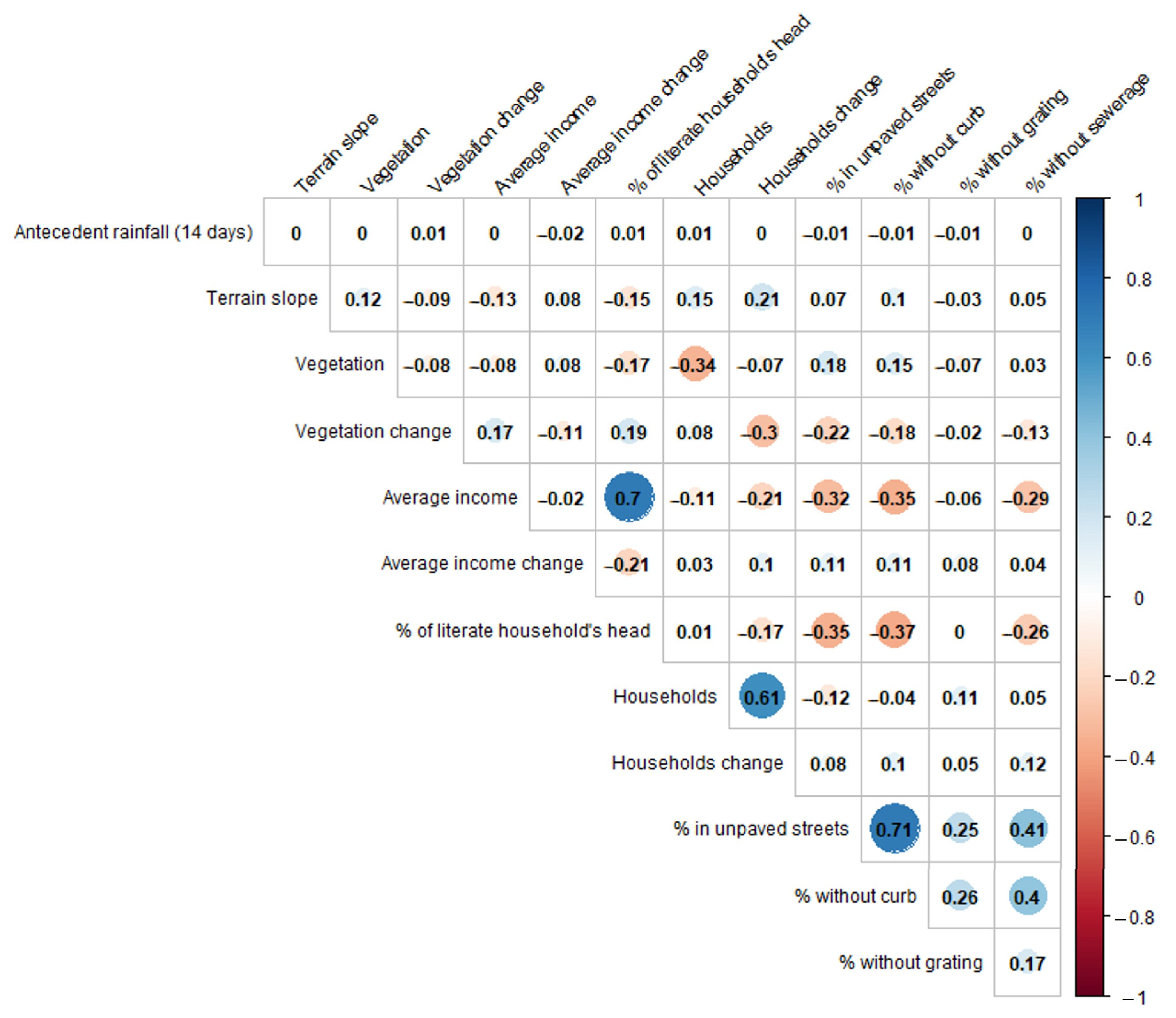
A correlation among variables was identified, although this was not used as a criterion for excluded variables. Among the continuous variables, a higher Spearman coefficient was found for average income of the household’s head and percentage of literate household heads; number of households in 2010 and household change between 1991 and 2010; and percentage of houses on unpaved streets and on streets without a storm sewer (curb). These are positive correlations, and they support the following: (a) households with a lower income are also households in which those responsible are less educated; (b) areas with a higher density of households presented a great increment between 1991 and 2010; and (c) streets without storm sewers (curbs) are frequently not paved. Both positive and inverse, less-intense correlations were also found (Figure A1).
Figure A1. Spearman correlation coefficients calculated for each pair of continuous variables.
Remotesensing 15 03048 g0a1
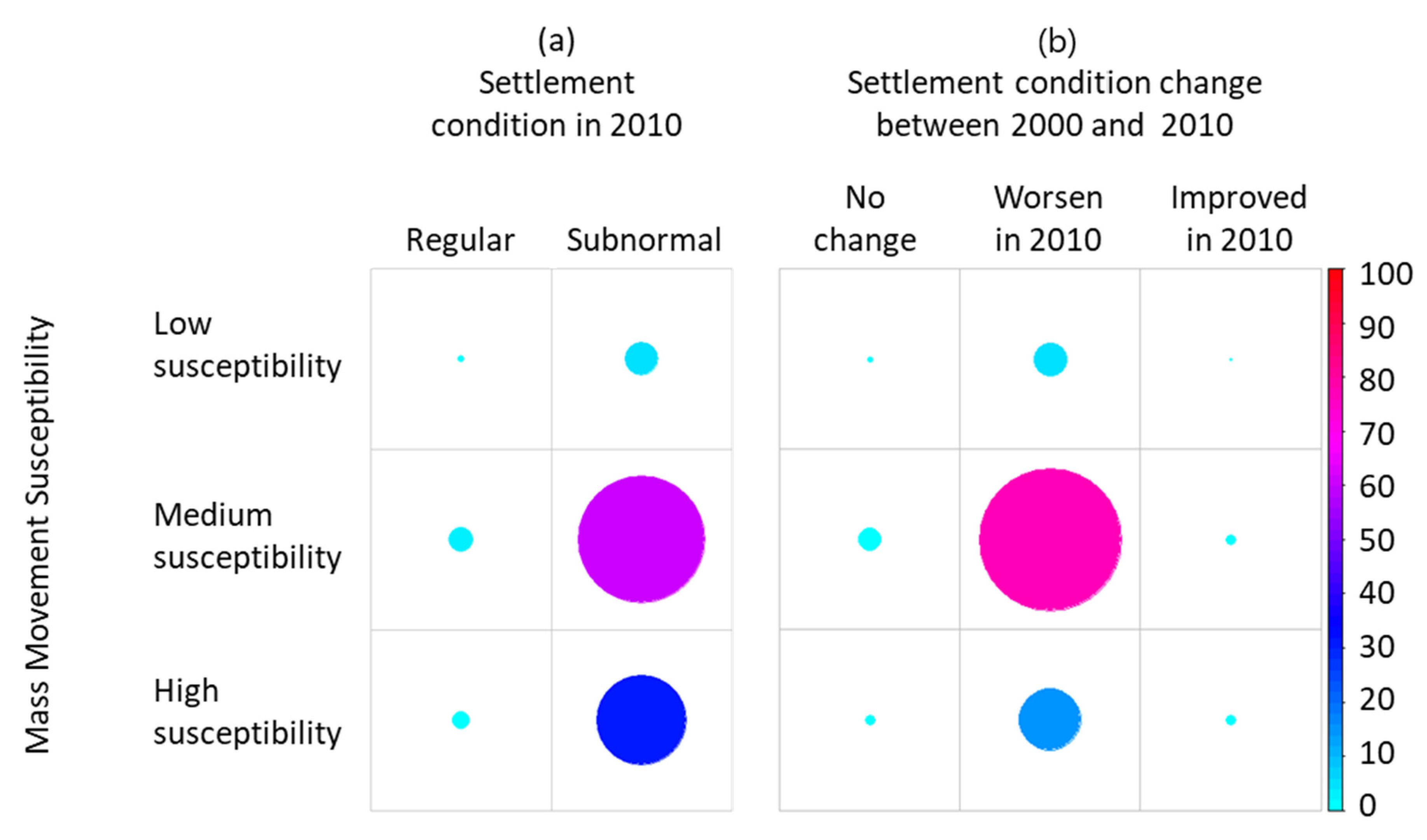
The categorical variables were dependent, according to Pearson’s chi-squared tests. The correlation between subnormal settlements in 2010 and the change in their conditions between 2000 and 2010 were expected. It is interesting to note the correlation between medium or high susceptibility to mass movement and subnormal areas (Figure A2a). These areas more prone to mass movements are also correlated with areas that became subnormal after 2000 (understood as a worsened situation in 2010) (Figure A2b).
Figure A2. Relative contribution to Pearson’s chi-squared test between mass movement susceptibility and (a) settlement condition in 2010 and (b) settlement condition change between 2000 and 2010.
Remotesensing 15 03048 g0a2
Finally, no significant correlation (i-value higher than 0.05 in F-statistic) was found between all possible pairs of a continuous variable and a categorical variable.

Appendix B. Model Development Results: Uni- and Multi-Variable Logistic Regression Assessment

Univariable models were calculated in order to select variables based on a p-value higher than 0.25. We then excluded two variables from further analyses: aspect and average, except average household head’s income change. For variables related to the percentage of households on streets without a storm sewer (curb) or with an open sewer, parameters yielded a p-value of 0.025 and 0.085, respectively, while for others, p-values associated with their parameters were lower than 0.001 (Table A3).
Table A3. Estimated coefficients, two-tailed p-values, 95% confidence intervals, and estimated likelihood ratios, χ2, for univariable logistic regression models.
Univariable ModelsInterceptCoefficientCoefficient Confidence Interval (95%)p-ValueLikelihood Ratio χ2
Antecedent rainfall (day and 14 previous days)−2.40340.0160[0.0160, 0.0161]<0.001911.7
Terrain slope−0.91480.0885[0.0882, 0.0888]<0.001296.3
Aspect0.1027 38.8
 North (in relation to flat areas) −0.0104[−0.0178, −0.0029]0.578
 East (in relation to flat areas) 0.4934[0.4858, 0.5010]0.008
 South (in relation to flat areas) 0.6820[0.6742, 0.6897]<0.001
 West (in relation to flat areas) 0.3958[0.3884, 0.4033]0.031
Mass movement susceptibility−0.1870 130.5
 Medium (in relation to low) 1.6395[1.6281, 1.6509]<0.001
 High (in relation to low) 1.9794[1.9579, 2.0008]<0.001
Percentage of vegetation in 2010−0.24451.6062[1.5976, 1.6148]<0.00194.0
Percentage of vegetation change0.15360.8527[0.8449, 0.8605]<0.00132.9
Average income of the household’s head in 20100.5021−0.0002[−0.0002, −0.0002]<0.00173.8
Average income change for the household’s head−0.023631−0.000021−0.000019]0.3901.7
Settlement condition in 2010−0.2097 162.4
 Subnormal (in relation to regular) 1.9845[1.9737, 1.9954]<0.001
Settlement condition change−0.0668 41.8
 Change (in relation to no change) 1.4055[1.3918, 1.4192]<0.001
Households in 2010−0.51840.0319[0.0316, 0.0321]<0.001102.1
Household change−0.21740.0289[0.0286, 0.0292]<0.00154.7
Percentage of households on streets without storm sewer (curb) in 2010−0.06150.5771[0.5666, 0.5876]0.0259.3
Percentage of households on streets without storm sewer (grating) in 20100.2189−0.5114[−0.5182, −0.5045]0.00316.2
Percentage of households on streets with open sewage in 20100.0384−0.7231[−0.7393, −0.7068]0.0855.7
Percentage of households without sewerage in 20100.1922−0.8958[−0.9032, −0.8884]<0.00138.8
In the complete model, where we analyzed the joint effects of variables, we excluded variables associated with a p-value > 0.05, which were those related to a change in conditions (vegetation change, subnormal settlement change, and household change), two variables related to the absence of infrastructure systems (percentage of households on streets with open sewage and percentage of households without storm sewers (grating)), and mass movement susceptibility (Table A4).
Table A4. Estimated coefficients, two-tailed p-values, and 95% confidence intervals, for the complete logistic regression model.
Variables of the Complete ModelCoefficientCoefficient
Confidence Interval (95%)
p-Value
Intercept−3.4228[−3.4369, −3.4087]<0.001
Antecedent rainfall (day and 14 previous days)0.0164[0.0164, 0.0165]<0.001
Terrain slope0.0608[0.0604, 0.0613]<0.001
Mass movement susceptibility
 Medium in relation to low0.2734[0.2573, 0.2894]0.399
 High in relation to low−0.0008[−0.0358, 0.0343]0.517
Percentage of vegetation in 20101.5938[1.5736, 1.6140]0,002
Percentage of vegetation change0.3379[0.3242, 0.3516]0.293
Average household head’s income in 2010−0.000123[−0.000125, −0.000121]0.012
Settlement condition in 20101.9657[1.9424, 1.9889]<0.001
Settlement condition change−0.9398[−0.9682, −0.9114]0.143
Households in 20100.0384[0.0379, 0.0390]0.002
Household change−0.0051[−0.0057, −0.0045]0.477
Percentage of households on streets without storm sewer (curb) in 20101.4845[1.4646, 1.5044]0.003
Percentage of households on streets without storm sewer (grating) in 2010−0.1482[−0.1598, −0.1365]0.468
Percentage of households on streets with open sewage in 2010−0.9120[−0.9394, −0.8846]0.182
Percentage of households without sewerage in 2010−1.6121[−1.6264, −1.5978]<0.001
Observations (n)
Points of landslide occurrence
Points of landslide non-occurrence
Bootstraps
2000
1000
1000
1000
Model likelihood test
Likelihood ratio χ2 d.f.
p-value
1301.8
15
<0.001

References

  1. Alexander, D. Urban landslides. Prog. Phys. Geogr. Earth Environ. 1989, 13, 157–189. [Google Scholar] [CrossRef]
  2. Burton, I.; Kates, R.W.; White, G.F. The Environment as Hazard, 2nd ed.; The Guilford Press: New York, NY, USA; London, UK, 1993; ISBN 0-89862-159-3. [Google Scholar]
  3. Horlick, J.T. Urban disasters and megacities in a Risk society. GeoJournal 1995, 37, 329–334. [Google Scholar] [CrossRef]
  4. United Nations Office for Disaster Risk Reduction (UNDRR). Global Assessment Report on Disaster Risk Reduction; Geneva, Switzerland, 2019. Available online: https://www.undrr.org/media/73965 (accessed on 16 July 2019).
  5. Alexander, D. On the causes of landslides: Human activities, perception, and natural processes. Environ. Geol. Water Sci. 1992, 20, 165–179. [Google Scholar] [CrossRef]
  6. Ren, D. The devastating Zhouqu storm-triggered debris flow of August 2010: Likely causes and possible trends in a future warming climate. J. Geophys. Res. Atmos. 2014, 119, 3643–3662. [Google Scholar] [CrossRef]
  7. EM-DAT. The OFDA/CRED International Disaster Database; Centre for Research on the Epidemiology of Disasters, Université Catholique de Louvain: Ottignies-Louvain-la-Neuve, Belgium, 2019. [Google Scholar]
  8. Cui, Y.; Cheng, D.; Choi, C.E.; Jin, W.; Lei, Y.; Kargel, J.S. The cost of rapid and haphazard urbanization: Lessons learned from the Freetown landslide disaster. Landslides 2019, 16, 1167–1176. [Google Scholar] [CrossRef] [Green Version]
  9. Froude, M.J.; Petley, D.N. Global fatal landslide occurrence from 2004 to 2016. Nat. Hazards Earth Syst. Sci. 2018, 18, 2161–2181. [Google Scholar] [CrossRef] [Green Version]
  10. Petley, D.N. On the impact of urban landslides. In Engineering Geology for Tomorrow’s Cities; Culshaw, M.G., Reeves, H.J., Jefferson, I., Spink, T.W., Eds.; Geological Society: London, UK, 2009; Volume 22, pp. 83–99. [Google Scholar] [CrossRef]
  11. United Nations—Department of Economic and Social Affairs-Population Division. The World’s Cities in 2018—Data Booklet (No. St/Esa/Ser.A/417); United Nations: New York, NY, USA, 2018. [Google Scholar]
  12. Ab’saber, A. O sítio urbano de São Paulo. In A Cidade de São Paulo—Estudos de Geografia Urbana; de Azevedo, A., Ed.; Cia. Editora Nacional: São Paulo, Brazil, 1958; Volume I, pp. 169–248. Available online: http://www.brasiliana.com.br/obras/a-cidade-de-spaulo-estudos-de-geografia-urbana-v01/preambulo/4/texto (accessed on 12 September 2017).
  13. Instituto Geológico (IG). Cadastro Georreferenciado de Eventos Geodinâmicos: 50 Municípios da Região Metropolitana de São Paulo, Baixada Santista e Litoral Norte; Instituto Geológico: São Paulo, Brazil, 2017. Available online: https://www.infraestruturameioambiente.sp.gov.br/wp-content/uploads/sites/233/2017/12/Cad_Desastres_Shapefile_50mun.zip (accessed on 16 June 2019).
  14. United Nations Office for Disaster Risk Reduction (UNDRR). Global Assessment Report on Disaster Risk Reduction; United Nations Office for Disaster Risk Reduction: Geneva, Switzerland, 2009; Available online: https://www.undrr.org/publication/global-assessment-report-disaster-risk-reduction-2009 (accessed on 16 July 2019).
  15. Ceped. Atlas Brasileiro de Desastres Naturais: 1991 a 2012, 2nd ed.; CEPED UFSC: Florianópolis, Brazil, 2013; ISBN 9788564695085. [Google Scholar]
  16. Srivastava, A.; Babu, G.L.S.; Haldar, S. Influence of Spatial Variability of Permeability Property on Steady State Seepage Flow and Slope Stability Analysis. Eng. Geol. 2009, 110, 93–101. [Google Scholar] [CrossRef]
  17. Stanley, T.; Kirschbaum, D.B. A Heuristic Approach to Global Landslide Susceptibility Mapping. Nat. Hazards 2017, 87, 145–164. [Google Scholar] [CrossRef] [Green Version]
  18. Budimir, M.E.A.; Atkinson, P.M.; Lewis, H.G. A systematic review of landslide probability mapping using logistic regression. Landslides 2015, 12, 419–436. [Google Scholar] [CrossRef] [Green Version]
  19. Miao, F.; Zao, F.; Wu, Y.; Li, L.; Török, A. Landslide Susceptibility Mapping in Three Gorges Reservoir Area Based on GIS and Boosting Decision Tree Model. Stoch. Environ. Res. Risk Assess. 2023, 37, 2283–2303. [Google Scholar] [CrossRef]
  20. Zhang, R.; Chen, Y.; Zhang, X.; Ma, Q.; Ren, L. Mapping Homogeneous Regions for Flash Floods Using Machine Learning: A Case Study in Jiangxi Province, China. Int. J. Appl. Earth Obs. Geoinf. 2022, 108, 102717. [Google Scholar] [CrossRef]
  21. Yao, J.; Zhang, X.; Luo, W.; Liu, C.; Ren, L. Applications of Stacking/Blending Ensemble Learning Approaches for Evaluating Flash Flood Susceptibility. Int. J. Appl. Earth Obs. Geoinf. 2022, 112, 102932. [Google Scholar] [CrossRef]
  22. Aksha, S.K.; Resler, L.M.; Juran, L.; Carstensen, L.W. A geospatial analysis of multi-hazard risk in Dharan, Nepal. Geomat. Nat. Hazards Risk 2020, 11, 88–111. [Google Scholar] [CrossRef] [Green Version]
  23. Zeng, J.; Zhu, Z.Y.; Zhang, J.L.; Ouyang, T.P.; Qiu, S.F.; Zou, Y.; Zeng, T. Social Vulnerability Assessment of Natural Hazards on County-Scale Using High Spatial Resolution Satellite Imagery: A Case Study in the Luogang District of Guangzhou, South China. Environ. Earth Sci. 2012, 65, 173–182. [Google Scholar] [CrossRef]
  24. Chang, H.; Pallathadka, A.; Sauer, J.; Grimm, N.B.; Zimmerman, R.; Cheng, C.; Iwaniec, D.M.; Kim, Y.; Lloyd, R.; McPhearson, T.; et al. Assessment of Urban Flood Vulnerability Using the Social-Ecological-Technological Systems Framework in Six Us Cities. Sustain. Cities Soc. 2021, 68, 102786. [Google Scholar] [CrossRef]
  25. Arrogante-Funes, P.; Bruzón, A.G.; Arrogante-Funes, F.; Ramos-Bernal, R.N.; Vázquez-Jiménez, R. Integration of Vulnerability and Hazard Factors for Landslide Risk Assessment. Int. J. Environ. Res. Public Health 2021, 18, 11987. [Google Scholar] [CrossRef]
  26. Ahmed, B. The Root Causes of Landslide Vulnerability in Bangladesh. Landslides 2021, 18, 1707–1720. [Google Scholar] [CrossRef]
  27. Kumar, D.; Bhattacharjya, R.K. Study of Integrated Social Vulnerability Index Sovi of Hilly Region of Uttarakhand, India. Environ. Clim. Technol. 2019, 24, 105–122. [Google Scholar] [CrossRef] [Green Version]
  28. Pickett, S.T.A.; Cadenasso, M.L.; Grove, J.M.; Boone, C.G.; Groffman, P.M.; Irwin, E.; Kaushal, S.S.; Marshall, V.; McGrath, B.P.; Nilon, C.H.; et al. Urban ecological systems: Scientific foundations and a decade of progress. J. Environ. Manag. 2011, 92, 331–362. [Google Scholar] [CrossRef] [PubMed]
  29. Mcphearson, T.; Haase, D.; Kabisch, N. Advancing understanding of the complex nature of urban systems. Ecol. Indic. 2016, 70, 566–573. [Google Scholar] [CrossRef]
  30. Depietri, Y.; Mcphearson, T. Integrating the Grey, Green, and Blue in Cities: Nature-Based Solutions for Climate Change Adaptation and Risk Reduction. In Nature-Based Solutions to Climate Change Adaptation in Urban Areas; Braubach, M., Egorov, A., Mudu, P., Wolf, T., Thompson, C.W., Martuzzi, M., Eds.; Springer: Berlin/Heidelberg, Germany, 2017. [Google Scholar] [CrossRef]
  31. Grabowski, Z.J.; Matsler, A.M.; Thiel, C.; Mcphillips, L.; Hum, R.; Bradshaw, A.; Redman, C. Infrastructures as Socio-Eco-Technical Systems: Five Considerations for Interdisciplinary Dialogue. J. Infrastruct. Syst. 2017, 23, 02517002. [Google Scholar] [CrossRef]
  32. Markolf, S.A.; Chester, M.V.; Eisenberg, D.A.; Iwaniec, D.M.; Davidson, C.I.; Zimmerman, R.; Chang, H. Interdependent Infrastructure as Linked Social, Ecological, and Technological Systems (SETSs) to Address Lock-in and Enhance Resilience. Earth’s Future 2018, 6, 1638–1659. [Google Scholar] [CrossRef] [Green Version]
  33. Mcphearson, T.; Pickett, S.T.A.; Grimm, N.B.; Niemelä, J.; Alberti, M.; Elmqvist, T.; Qureshi, S. Advancing Urban Ecology toward a Science of Cities. BioScience 2016, 66, 198–212. [Google Scholar] [CrossRef] [Green Version]
  34. Bai, X.; Surveyer, A.; Elmqvist, T.; Gatzweiler, F.W.; Güneralp, B.; Parnell, S.; Webb, R. Defining and advancing a systems approach for sustainable cities. Curr. Opin. Environ. Sustain. 2016, 23, 69–78. [Google Scholar] [CrossRef]
  35. Guidicini, G.; Iwasa, O.Y. Tentative correlation between rainfall and landslides in a humid tropical environment. Bull. Int. Assoc. Eng. Geol. 1977, 16, 13–20. [Google Scholar] [CrossRef]
  36. Schuster, R.L.; Highland, L.M. The Third Hans Cloos Lecture. Urban landslides: Socioeconomic impacts and overview of Mitigative strategies. Bull. Eng. Geol. Environ. 2007, 66, 1–27. [Google Scholar] [CrossRef]
  37. Ávila, A.; Justino, F.; Wilson, A.; Bromwich, D.; Amorim, M. Recent precipitation trends, flash floods and landslides in southern Brazil. Environ. Res. Lett. 2016, 11, 114029. [Google Scholar] [CrossRef]
  38. Segoni, S.; Piciullo, L.; Gariano, S.L. A review of the recent literature on rainfall thresholds for landslide occurrence. Landslides 2018, 15, 1483–1501. [Google Scholar] [CrossRef]
  39. Dai, F.C.; Lee, C.F. A spatiotemporal probabilistic modelling of storm-induced shallow landsliding using aerial photographs and logistic regression. Earth Surf. Process. Landf. 2003, 28, 527–545. [Google Scholar] [CrossRef]
  40. Santoro, J.; Mendes, R.M.; Pressinotti, M.M.N.; Manoel, G.R. Correlação Entre Chuvas e Deslizamentos Ocorridos Durante a Operação do Plano Preventivo De Defesa Civil. In Proceedings of the 7th Simpósio Brasileiro de Cartografia Geotécnica e Geoambiental, Maringá, Brazil, 8–11 August 2010. [Google Scholar]
  41. Tatizana, C.; Ogura, A.T.; Cerri, L.E.S.; Rocha, M.C.M. Modelamento numérico da análise de correlação entre chuvas e escorregamentos aplicado às encostas da Serra do Mar no município de Cubatão. In Proceedings of the 5th Congresso Brasileiro de Geologia de Engenharia; ABGE: São Paulo, Brazil, 1987; Volume 2, pp. 237–248. [Google Scholar]
  42. Pasuto, A.; Silvano, S. Rainfall as a trigger of shallow mass movements. A case study in the Dolomites, Italy. Environ. Geol. 1998, 35, 184–189. [Google Scholar] [CrossRef]
  43. Mendes, R.M.; de Andrade, M.R.M.; Tomasella, J.; de Moraes, M.A.E.; Scofield, G.B. Understanding shallow landslides in Campos do Jordão municipality-Brazil: Disentangling the anthropic effects from natural causes in the disaster of 2000. Nat. Hazards Earth Syst. Sci. 2018, 18, 15–30. [Google Scholar] [CrossRef] [Green Version]
  44. Guzzetti, F.; Reichenbach, P.; Bartoccini, P.; Galli, M.; Ardizzone, F.; Cardinali, M. Rainfall induced landslides in December 2004 in south-western Umbria, central Italy: Types, extent, damage and risk assessment. Nat. Hazards Earth Syst. Sci. 2006, 6, 237–260. [Google Scholar]
  45. Kirschbaum, D.; Stanley, T. Satellite-Based Assessment of Rainfall-Triggered Landslide Hazard for Situational Awareness. Earth’s Future 2018, 6, 505–523. [Google Scholar] [CrossRef] [PubMed]
  46. Guzzetti, F.; Peruccacci, S.; Rossi, M.; Stark, C.P. Rainfall thresholds for the initiation of landslides in central and southern Europe. Meteorol. Atmos. Phys. 2007, 98, 239–267. [Google Scholar] [CrossRef]
  47. Instituto Geológico (IG). Relatório Da Operação Dos Planos Preventivos De Defesa Civil—PPDC: Operação Verão 2016–2017; Instituto Geológico: São Paulo, Brazil, 2017. Available online: https://www.infraestruturameioambiente.sp.gov.br/wp-content/uploads/sites/233/2017/11/RELAT_PPDC_2016-2017_FINAL.pdf (accessed on 15 June 2019).
  48. Ahrendt, A.; Zuquette, L.V. Triggering factors of landslides in Campos do Jordão city, Brazil. Bull. Eng. Geol. Environ. 2003, 62, 231–244. [Google Scholar] [CrossRef]
  49. Smyth, C.G.; Royle, S.A. Urban landslide hazards: Incidence and causative factors in Niteroi, Rio de Janeiro state, Brazil. Appl. Geogr. 2000, 20, 95–118. [Google Scholar] [CrossRef]
  50. Chau, K.T.; Chan, J.E. Regional bias of landslide data in generating susceptibility maps using logistic regression: Case of Hong Kong Island. Landslides 2005, 2, 280–290. [Google Scholar] [CrossRef]
  51. Süzen, M.L.; Kaya, B.Ş. Evaluation of environmental parameters in logistic regression models for landslide susceptibility mapping. Int. J. Digit. Earth 2012, 5, 338–355. [Google Scholar] [CrossRef]
  52. Varnes, D.J. Slope Movement Types and Processes (special report No. 176). In Landslides: Analysis and Control; Schuster, R.L., Krizek, R.J., Eds.; Transportation Research Board, National Research Council: Washington, DC, USA, 1978. [Google Scholar]
  53. Bitar, O.Y. (Ed.) Cartas de Susceptibilidade a Movimentos Gravitacionais de Massa e Inundações—1:25.000: Nota Técnica Explicativa; Instituto de Pesquisas Tecnológicas do Estado de São Paulo (IPT): São Paulo, Brazil; Serviço Geológico do Brasil (CPRM): Brasília, Brazil, 2014. [Google Scholar]
  54. Kanungo, D.; Arora, M.; Sarkar, S.; Gupta, R. Landslide Susceptibility Zonation (LSZ) Mapping–A Review. J. South Asia Disaster Stud. 2009, 2, 81–105. [Google Scholar]
  55. Ross, J.L.S. Inundações e deslizamentos em São Paulo: Riscos da relação inadequada sociedade-natureza. Territorium 2016, 8, 15–23. [Google Scholar] [CrossRef] [Green Version]
  56. Alexander, D. Vulnerability to Landslides. In Landslide Hazard and Risk; Glade, T., Anderson, M., Crozier, M.J., Eds.; John Wiley & Sons, Ltd.: Hoboken, NJ, USA, 2005; pp. 175–198. [Google Scholar] [CrossRef]
  57. Imaizumi, F.; Sidle, R.C.; Kamei, R. Effects of forest harvesting on the occurrence of landslides and debris flows in steep terrain of central Japan. Earth Surf. Process. Landf. 2008, 33, 827–840. [Google Scholar] [CrossRef]
  58. Peloggia, A.U.G. Delineação e Aprofundamento Temático da Geologia do Tecnógeno do Município de São Paulo. Ph.D. Thesis, Universidade de São Paulo, Instituto de Geociências, São Paulo, Brazil, 1997. [Google Scholar]
  59. Mirandola, F.A.; de Macedo, E.S. Proposta de classificação do tecnógeno para uso no mapeamento de áreas de risco de deslizamento. Quat. Environ. Geosci. 2014, 5, 66–81. [Google Scholar] [CrossRef]
  60. Blaikie, P.; Cannon, T.; Davis, I.; Wisner, B. At Risk: Natural Hazards, People’s Vulnerability and Disasters; Routledge: London, UK, 1994. [Google Scholar] [CrossRef]
  61. Peloggia, A.U.G.; Silva, F.A.N.; Takyia, H.; Barros, L.H.S.; Fujimoto, N.A.; Figueiredo, R.B. Riscos geológicos e geotécnicos em áreas de precária ocupação urbana no município de São Paulo; Sociedade Brasileira de Geologia: São Paulo, Brazil, 1992. [Google Scholar] [CrossRef]
  62. Farah, F. Habitação e Encostas; Instituto de Pesquisas Tecnológicas: São Paulo, Brazil, 2003; Publicação IPT; p. 2795. [Google Scholar]
  63. Marcondes, M.J.D.A. Cidade e Natureza. Proteção dos Mananciais e Exclusão Social, 1st ed.; Studio Nobel, Edusp, Fapesp: São Paulo, Brazil, 1999. [Google Scholar]
  64. Instituto Brasileiro de Geografia e Estatística (IBGE). Manual Técnico de Geomorfologia (Manuais Técnicos em Geociências No. 5); Instituto Brasileiro de Geografia e Estatística: Rio de Janeiro, Brazil, 2009; ISBN 9788524042225. [Google Scholar]
  65. Empresa Paulista de Planejamento Metropolitano S.A. (EMPLASA). Folhas Planialtimétricas da Região Metropolitana de São Paulo—1980/1981 (com atualizações); EMPLASA: São Paulo, Brazil, 1980; Scale: 1:10.000. [Google Scholar]
  66. Sepe, P.M.; Takiya, H. Atlas Ambiental da Cidade de São Paulo; Secretaria Municipal do Verde e do Meio Ambiente (SVMA): São Paulo, Brazil, 2000. [Google Scholar]
  67. Nobre, C.A.; Young, A.F.; Saldiva, P.H.N.; Orsini, J.A.M.; Nobre, A.D.; Ogura, A.; Rodrigues, G.D.O. Vulnerabilidades das Megacidades Brasileiras às Mudanças Climáticas: Região Metropolitana de São Paulo; Instituto Nacional de Pesquisas Espaciais: São José dos Campos, Brazil; Universidade Estadual de Campinas: Campinas, Brazil, 2011. [Google Scholar]
  68. Xavier, T.M.B.S.; Xavier, A.F.S.; Silva Dias, M.A.F.D. Evolução da precipitação diária num ambiente urbano: O caso da cidade de São Paulo. Rev. Bras. Meteorol. 1994, 9, 44–53. [Google Scholar]
  69. Funk, C.; Peterson, P.; Landsfeld, M.; Pedreros, D.; Verdin, J.; Shukla, S.; Husak, G.; Rowland, J.; Harrison, L.; Hoell, A.; et al. The climate hazards infrared precipitation with stations - A new environmental record for monitoring extremes. Sci. Data 2015, 2, 150066. [Google Scholar] [CrossRef] [Green Version]
  70. Horn, B.K.P. Hill-Shading and the Reflectance Map. Proc. IEEE 1981, 69, 14–47. [Google Scholar] [CrossRef] [Green Version]
  71. Instituto Brasileiro de Geografia e Estatística (IBGE). Censo Demográfico 1991 (No. 21); Instituto Brasileiro de Geografia e Estatística: Rio de Janeiro, Brazil, 1991. Available online: https://www.ibge.gov.br/estatisticas/sociais/populacao/25089-censo-1991-6.html?edicao=25090 (accessed on 18 June 2019).
  72. Instituto Brasileiro de Geografia e Estatística (IBGE). Metodologia do Censo Demográfico 2010 (Série Relatórios Metodológicos No. 41; Série Relatórios Metodológicos (Vol. 41); Instituto Brasileiro de Geografia e Estatística: Rio de Janeiro, Brazil, 2013. [Google Scholar]
  73. Joint Research Centre (JRC)—European Commission. Documentation for the GHS Population Grid, Derived from Gpw4, Multitemporal (1975, 1990, 2000, 2015) (GHS-Pop); European Commission: Ispra, Italy, 2017. [Google Scholar]
  74. Langford, M.; Unwin, D.J. Generating and mapping population density surfaces within a geographical information system. Cartogr. J. 1994, 31, 21–26. [Google Scholar] [CrossRef] [PubMed]
  75. Holt, J.B.; Lo, C.P.; Hodler, T.W. Dasymetric Estimation of Population Density and Areal Interpolation of Census Data. Cartogr. Geogr. Inf. Sci. 2004, 31, 103–121. [Google Scholar] [CrossRef]
  76. Hirye, M.C.M.; McPhearson, T.; Filardo Jr., A.S.; Alves, D.S. Demographic, economic and physical data integration: Measuring hillside’s urban occupation in Metropolitan Region of São Paulo (Brazil). In Proceedings of the Proceedings American Geophysical Union Fall Meeting 2018, Washington, DC, USA, 10–14 December 2018. Abstract Number IN33B-0859. [Google Scholar]
  77. Fell, R.; Whitt, G.; Miner, T.; Flentje, P. Guidelines for landslide susceptibility, hazard and risk zoning for land use planning. Eng. Geol. 2008, 102, 83–84. [Google Scholar] [CrossRef] [Green Version]
  78. Glade, T.; Crozier, M.J. Landslide Hazard and Risk—Concluding Comment and Perspectives. In Landslide Hazard and Risk; Glade, T., Anderson, M., Crozier, M.J., Eds.; John Wiley & Sons, Ltd.: Chichester, England, 2005; pp. 765–774. [Google Scholar] [CrossRef]
  79. Van Westen, C.J.; Castellanos, E.; Kuriakose, S.L. Spatial data for landslide susceptibility, hazard, and vulnerability assessment: An overview. Eng. Geol. 2008, 102, 112–131. [Google Scholar] [CrossRef]
  80. Brenning, A. Spatial prediction models for landslide hazards: Review, comparison and evaluation. Nat. Hazards Earth Syst. Sci. 2005, 5, 853–862. [Google Scholar] [CrossRef]
  81. Steyerberg, E.W.; Harrell, F.E.; Borsboom, G.J.J.; Eijkemans, M.J.; Vergouwe, Y.; Habbema, J.D.F. Internal validation of predictive models: Efficiency of some procedures for logistic regression analysis. J. Clin. Epidemiol. 2001, 54, 774–781. [Google Scholar] [CrossRef] [PubMed]
  82. Efron, B.; Robert, J.T. An Introduction to the Bootstrap; Chapman & Hall/Crc: Boca Raton, FL, USA, 1994. [Google Scholar]
  83. Harrell, F.E. Regression Modeling Strategies; Springer International Publishing: Cham, Switzerland, 2015. [Google Scholar] [CrossRef]
  84. Hosmer, D.W.; Lemeshow, S. Applied Logistic Regression, 2nd ed.; John Wiley & Sons, Inc.: Hoboken, NJ, USA, 2000. [Google Scholar]
  85. Smith, T.J.; Mckenna, C.M. A comparison of logistic regression pseudo R2 indices. Mult. Linear Regres. Viewp. 2013, 39, 17–26. [Google Scholar]
  86. Schwarz, G. Estimating the Dimension of a Model. Ann. Stat. 1978, 6, 461–464. [Google Scholar] [CrossRef]
  87. Kirschbaum, D.; Kapnick, S.B.; Stanley, T.; Pascale, S. Changes in Extreme Precipitation and Landslides Over High Mountain Asia. Geophys. Res. Lett. 2020, 47. [Google Scholar] [CrossRef]
  88. El Kharim, Y.; Bounab, A.; Ilias, O.; Hilali, F.; Ahniche, M. Landslides in the urban and suburban perimeter of Chefchaouen (Rif, Northern Morocco): Inventory and case study. Nat. Hazards 2021, 107, 355–373. [Google Scholar] [CrossRef]
  89. Ehrlich, M.; Luiz, B.J.; Mendes, C.G.; Lacerda, W.A. Triggering factors and critical thresholds for landslides in Rio de Janeiro-Rj, Brazil. Nat. Hazards 2021, 107, 937–952. [Google Scholar] [CrossRef]
  90. Bezerra, L.; Neto, O.D.F.; Santos, O., Jr.; Mickovski, S. Landslide Risk Mapping in an Urban Area of the City of Natal, Brazil. Sustainability 2020, 12, 9601. [Google Scholar] [CrossRef]
  91. Cascini, L.; Bonnard, C.; Corominas, J.; Jibson, R.W.; Montero-Olarte, J. Landslide risk evaluation and hazard zoning for rapid and long-travel landslides in urban development areas. In Landslide Risk Management; Taylor and Francis: London, UK, 2005; pp. 199–235. [Google Scholar] [CrossRef]
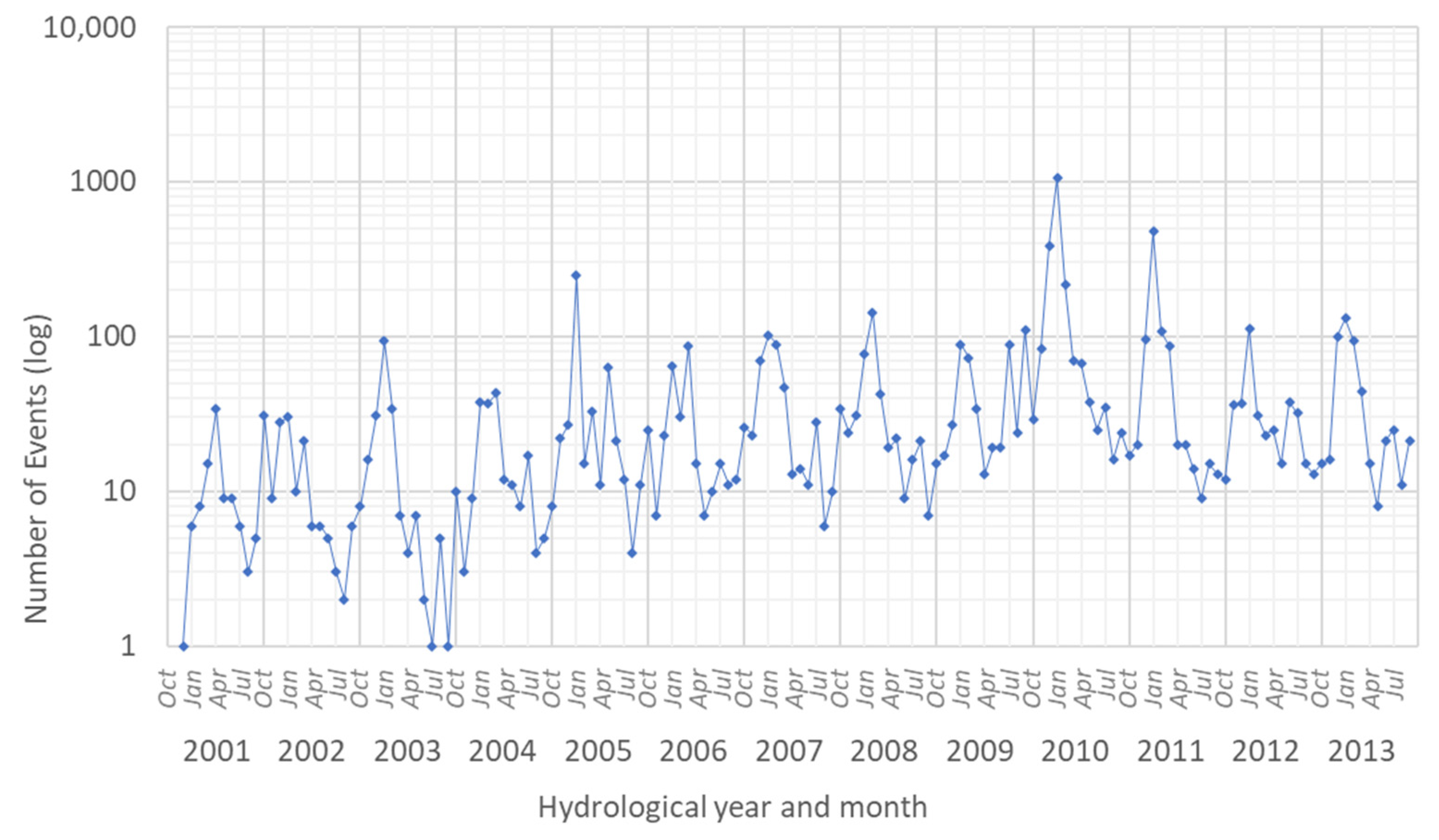
Figure 1. Recorded landslide events from 2001 to 2013 in the MRSP from the Inventory of Geodynamic Events [13].
Remotesensing 15 03048 g001
Figure 2. Common self-aided practices in informal settlements: (a) building houses; (b) terrain cut.
Remotesensing 15 03048 g002
Figure 3. Dense urban development of hillsides in the MRSP: (a) a general overview of Jardim Paraná, a low-income neighborhood on the hillsides of Cantareira Mountain Ridge, in São Paulo city; (b) looking to the opposite side of Jardim Paraná, a new favela is forming, where houses are substituting native vegetation cover.
Remotesensing 15 03048 g003
Figure 4. Urban occupation and geomorphological domains in the MRSP.
Remotesensing 15 03048 g004
Figure 5. Likelihood chi-squared test values for univariable models of antecedent rainfall computed with periods from 1 to 120 days.
Remotesensing 15 03048 g005
Table 1. Independent variables selected to model the occurrence of landslides in the MRSP.
DomainIndependent Variable
Ecological–Biophysical DomainDaily rainfall
Antecedent rainfall
Terrain slope
Terrain aspect
Mass movement susceptibility
Percentage of vegetation in 2010
Percentage of vegetation change (2010–1991)
Social–Behavioral DomainAverage income of the individual responsible for the household in 2010
Average change in income of the individual responsible for the household (2010–1991)
Percentage of literate individuals responsible for the household (household’s head) in 2010
Settlement condition in 2010
Settlement condition change (2010–1991)
Technological–Infrastructural DomainHouseholds in 2010
Household changes (2010–1991)
Percentage of households without sewerage in 2010
Percentage of households on unpaved streets in 2010
Percentage of households on streets without storm sewer (curb) in 2010
Percentage of households on streets without storm sewer (grating) in 2010
Percentage of households on streets with open sewage in 2010
Table 2. Estimated coefficients, two-tailed p-values, and 95% confidence intervals for the final logistic regression model.
Variables of Final ModelCoefficientCoefficient Confidence Interval (95%)p-Value
Intercept−3.5869[−3.5997, −3.5740]<0.001
Antecedent rainfall (day and 14 previous days)0.0163[0.0162, 0.0163]<0.001
Terrain slope0.0621[0.0617, 0.0625]<0.001
Percentage of vegetation in 20101.7894[1.7699, 1.8089]<0.001
Average household head’s income in 2010 −0.0001[−0.0001, −0.0001]0.019
Settlement condition in 20101.5335[1.5180, 1.5489]<0.001
Households in 20100.0370[0.0365, 0.0374]<0.001
Percentage of households on streets without storm sewer (curb) in 20101.1494[1.1329, 1.1659]0.007
Percentage of households without sewerage in 2010−1.7180[−1.7317, −1.7044]<0.001
Final model
Observations (n)
Points of landslide occurrence
Points of landslide non-occurrence
Bootstraps

2000
1000
1000
1000
Model likelihood test
Likelihood ratio χ2 d.f.
p-value
1280.3
8
<0.001
Table 3. Top three ranked models according to Bayesian information criterion (BIC).
Final Model and
Models with Subset of Selected Variables
RankNumber of Times as Rank #1BIC ValueBIC Value
Confidence Interval (95%)
Final model15491561[1559, 1564]
Final model, except average household head’s income in 201022741557[1554, 1559]
Final model, except percentage of households on streets without storm sewer (curb) in 201031551559[1556, 1562]
Table 4. Index of adequacy of each variable of the final logistic regression model.
VariableLikelihood Ratio χ2Adequacy
Antecedent rainfall (day and 14 previous days)900.60.70
Terrain slope262.20.20
Percentage of vegetation in 201020.70.02
Average household head’s income in 2010 73.70.06
Settlement condition in 2010191.30.15
Households in 2010174.90.14
Percentage of households on streets without storm sewer (curb) in 201016.90.01
Percentage of households without sewerage in 201024.50.02
Combined1280.31.00
Table 5. Index of adequacy of each variable of the final logistic regression model.
VariableIncrementOdds RatioOdds Ratio Confidence Interval (95%)
Antecedent rainfall (day and 14 previous days)10 mm1.177[1.176, 1.177]
Terrain slope1.064[1.064, 1.065]
Percentage of vegetation in 201010%1.196[1.194, 1.199]
Average household head’s income in 2010 BRL 10,0000.989[0.9887, 0.9891]
Settlement condition in 2010Subnormal in relation to regular4.634[4.705, 4.863]
Households in 20101 household1.038[1.037, 1.038]
Percentage of households on streets without storm sewer (curb) in 201010%1.122[1.120, 1.124]
Percentage of households without sewerage in 201010%0.842[0.841, 0.843]
Disclaimer/Publisher’s Note: The statements, opinions and data contained in all publications are solely those of the individual author(s) and contributor(s) and not of MDPI and/or the editor(s). MDPI and/or the editor(s) disclaim responsibility for any injury to people or property resulting from any ideas, methods, instructions or products referred to in the content.