Semi-Supervised Classification for Intra-Pulse Modulation of Radar Emitter Signals Using Convolutional Neural Network

Abstract

Intra-pulse modulation classification of radar emitter signals is beneficial in analyzing radar systems. Recently, convolutional neural networks (CNNs) have been used in classification of intra-pulse modulation of radar emitter signals, and the results proved better than the traditional methods. However, there is a key disadvantage in these CNN-based methods: the CNN requires enough labeled samples. Labeling the modulations of radar emitter signal samples requires a tremendous amount of prior knowledge and human resources. In many circumstances, the labeled samples are quite limited compared with the unlabeled samples, which means that the classification will be semi-supervised. In this paper, we propose a method which could adapt the CNN-based intra-pulse classification approach to the case where a very limited number of labeled samples and a large number of unlabeled samples are provided, to classify the intra-pulse modulations of radar emitter signals. The method is based on a one-dimensional CNN and uses pseudo labels and self-paced data augmentation, which could improve the accuracy of intra-pulse classification. Extensive experiments show that our proposed method can improve the intra-pulse modulation classification performance in the semi-supervised situations.

1. Introduction

Intra-pulse modulation classification of radar emitter signals is a key technology in electronic support measure systems, electronic intelligence systems and radar warning receivers [1,2,3] that is beneficial in analyzing radar systems. The accurate classification of the intra-pulse modulation of radar emitter signals could increase the reliability of estimating the function of the radar and indicate the presence of a potential threat, such that necessary measures or countermeasures against enemy radars could be taken by the ELINT system [4].

In recent years, deep learning [5] has attracted great attention in the field of artificial intelligence. Some deep-learning-based methods, especially convolutional neural networks (CNNs) [6,7,8,9,10,11], have been applied in many tasks in radar systems, such as synthetic aperture radar (SAR) automatic target recognition [12]. Apart from this, they have been used in intra-pulse modulation classification of radar emitter signals. In [13], Kong et al. used Choi−Williams Distribution (CWD) images of low probability of intercept (LPI) radar signals and recognized the intra-pulse modulations. Similarly, Yu et al. [14] obtained time-frequency images (TFIs) of the radar signal using CWD and extracted the contour of the signal in the TFIs. After that, a CNN model was trained with the contour images. In [15], Zhang et al. used Wigner−Ville Distribution (WVD) images of radar signals, which contained five types of intra-pulse modulations, to train the CNN model. In [16], Huynh-The et al. designed a cost-efficient convolutional neural network which could learn the spatiotemporal signal correlations via different asymmetric convolution kernels to classify automatic modulation classification. In [17], Peng et al. used two CNN models and three conventional machine-learning-based methods to classify the modulations, and the results show that CNN models are superior to other machine-learning-based methods. In [18], Yu et al. firstly preprocessed the radar signal by Short-Time Fourier Transformation (STFT), and then a CNN model was trained to classify the intra-pulse modulation of the radar signals. These methods mentioned above are based on a two-dimensional (2-D) CNN model. In terms of the dimension of radar signals, one-dimensional (1-D) CNN-based method are more suitable to classify the modulations task. Wu et al. [19] designed a 1-D CNN with an attention mechanism to recognize seven types of radar emitter signals in the time domain, where the intra-pulse modulations of the signals are different. In our previous work [20], a 1-D Selective Kernel Convolutional Neural Network (SKCNN) was proposed to classify eleven types of intra-pulse modulations of radar emitter signals. According to our experimental results, the proposed method based on 1-D SKCNN has the advantage of faster speed in data preprocessing and higher accuracy in intra-pulse modulation classification of radar emitter signals.

For the methods mentioned above, the performance of the CNN models depends on the number of labeled samples. The similarity among these methods is that the labeled samples are enough. However, labeling the radar emitter signal samples requires a tremendous amount of prior knowledge and human resources, such as a probability model or some other parameters of the signals including spectrum autocorrelation, time-frequency analysis, high-order cumulants and various transform domain analyses, which increases the difficulty of labeling and leads to a situation in which the labeled samples are quite limited. In the real application of classification intra-pulse modulations of radar emitter signals, unlabeled samples are much greater than the labeled samples. Therefore, the original fully supervised classification tasks often do not exist, and tasks will be semi-supervised. Semi-supervised tasks have been widely studied in image classification. In [21], Lee proposed a pseudo label learning method for deep neural networks, which shows a state-of-the-art performance in the MNIST dataset. In [22], the authors produced a new algorithm called MixMatch by guessing low-entropy labels for data-augmented unlabeled examples and mixing labeled and unlabeled data using MixUp, which reduced the error rate from 38% to 11% in the CIFAR-10 dataset. In [23], the authors simplified the existing semi-supervised methods and proposed FixMatch by using the pseudo labels generated from the weakly augmented unlabeled samples and the corresponding strongly augmented samples to train a CNN model, which combined the techniques of pseudo label learning and consistency regularization [24,25,26]. The experimental results show that FixMatch achieved state-of-the-art performance across a variety of standard semi-supervised learning benchmarks.

For intra-pulse modulation classification of radar emitter signals, most of the deep-learning-based methods focus on the fully supervised cases. As a result, in this paper, we have proposed a method to classify the intra-pulse modulation of radar emitter signals in the case where a very limited number of labeled samples and a large number of unlabeled samples are provided. The method uses the techniques of a CNN based on a mixed attention mechanism, pseudo labels and self-paced data augmentation, which could improve the accuracy for intra-pulse classification. The method could classify eleven types of intra-pulse modulations signals, including single-carrier frequency (SCF) signals, linear frequency modulation (LFM) signals, sinusoidal frequency modulation (SFM) signals, binary frequency shift keying (BFSK) signals, quadrature frequency shift keying (QFSK) signals, even quadratic frequency modulation (EQFM) signals, dual frequency modulation (DLFM) signals, multiple linear frequency modulation (MLFM) signals, binary phase shift keying (BPSK) signals, Frank phase-coded (Frank) signals, and composite modulation of LFM and BPSK (LFM-BPSK) signals.

The main contribution of this paper is that unlike most of the fully supervised situations, we focus on a more common semi-supervised situation, where a very limited number of labeled samples and a large number of unlabeled samples are provided. Another contribution is that our method is based on a one-dimensional CNN, and it uses pseudo labels and self-paced data augmentation, which could improve the accuracy for intra-pulse classification. The specific results can be seen in Section 4 and Section 5.

This paper is organized as follows: In Section 2, the proposed method will be introduced in detail. The dataset and setting of parameters will be shown in Section 3. The extensive experiments and corresponding analysis will be carried out in Section 4. The ablation study and application scenarios will be given in Section 5. Finally, the conclusion will be presented in Section 6.

2. The Proposed Method

Semi-supervised classification for intra-pulse modulation of radar emitter signals refers to the case in which a very limited number of labeled samples and a huge number of unlabeled samples are provided. For an L-class classification problem, let $X=\{(x_b,y_b):b\in (1,\dots ,B)\}$ be $B$ labeled samples, where $x_b$ are the training samples and $y_b$ are true labels. Let $U=\{u_{b^{\prime }}:b^{\prime }\in (1,\dots ,B^{\prime })\}$ be $B^{\prime }$ labeled samples, where $u_{b^{\prime }}$ are the unlabeled samples, and $B^{\prime }$ is always much larger than $B$. In this paper, the method mainly consists of the following steps:

(1)

Preprocess the original raw radar emitter signal samples.

(2)

Generate pseudo labels of unlabeled samples and their confidence. Select the high-confidence unlabeled samples.

(3)

Make self-paced data augmentation for the selected unlabeled samples. Train the CNN model with the true-label samples and the selected pseudo-label samples.

The flow chart of our proposed method is provided in Figure 1, where the parts linked by red arrow are executed only once, and the parts in the black circle will be executed several times. Finally, the well-trained CNN will be obtained for the testing sessions.

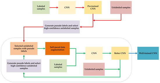
Figure 1. The flow chart of our proposed method.

2.1. The Structure of CNN

It is widely known that a more complicated CNN model such as VGG network or ResNet, where the depth, floating point operations and parameters of the model are very high, could bring about better classification results. However, the training cost would be huge. As radar systems have higher real-time requirements, the model should be light-weighted. Attention mechanisms have been widely used in CNN model designing for their light-weighted structure, for instance, channel attention [27] and spatial attention [28]. In addition, inspired by our previous work in [20], which employed different scales of convolutional kernel size, in this paper, we design a light-weighted CNN model (MA-CNN) with mixed attention mechanism as the classification backbones, where the attention features are extracted by multi-scale components. The structure of the proposed MA-CNN and the structure of the mixed attention block is shown in Figure 2 and Figure 3, respectively.

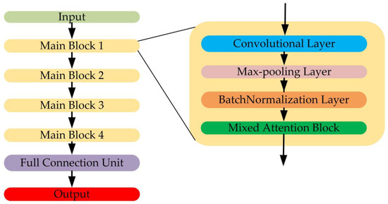
Figure 2. The structure of mixed attention convolutional neural network (MA-CNN).

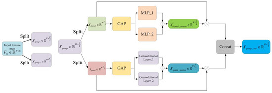
Figure 3. The structure of mixed attention block.

The MA-CNN contains four main blocks, and each block contains a convolutional layer with a “ReLU” activation function [29], a Max-Pooling layer, a batch-normalization layer [30] and a mixed attention block. The details of the MA-CNN will be introduced in Section 3.2.

In the mixed attention block, for a given input feature map $F_{in}\in {ℝ}^{W\times C}$, where $W$ is the length and $C$ is the number of channel, firstly, $F_{in}$ is split into two groups, $X_{group1}\in {ℝ}^{W\times \frac{C}{2}}$ and $X_{group2}\in {ℝ}^{W\times \frac{C}{2}}$, in a channel-wise way. Then, each group is split channel-wise into two parts named $X_{channel}\in {ℝ}^{W\times \frac{C}{4}}$ and $X_{spatial}\in {ℝ}^{W\times \frac{C}{4}}$.

For the $X_{channel}$, we extract the channel attention by fusing the output of two different Multi-Layer Perceptrons (MLPs). This process can be written as:

$$X_{channel\_attention}=\mathrm{MLP}\_1({\mathrm{GAP}}^s(X_{group}))+\mathrm{MLP}\_2({\mathrm{GAP}}^s(X_{group}))$$

(1)

where $X_{channel\_attention}\in {ℝ}^{1\times \frac{C}{4}}$, $\mathrm{MLP}\_1(\cdot )$ and $\mathrm{MLP}\_2(\cdot )$ refer to the two MLPs with different nodes in the hidden layer. ${\mathrm{GAP}}^s(\cdot )$ refers to global average pooling in a wide-wise way. $X_{group}$ refers to $X_{group1}$ or $X_{group2}$.

Similarly, for the $X_{spatial}$, we extract the spatial attention by fusing the output of two different convolutional layers. This process could be written as:

$$X_{spatial\_attention}=\mathrm{Conv}\text{\_}1({\mathrm{GAP}}^{\mathrm{c}}(X_{group}))+\mathrm{Conv}\text{\_}2({\mathrm{GAP}}^{\mathrm{c}}(X_{group}))$$

(2)

where $X_{spatial\_attention}\in {ℝ}^{W\times 1}$, ${\mathrm{GAP}}^s(\cdot )$ refers to global average pooling in a channel-wise way.$\mathrm{Conv}\_1(\cdot )$ and $\mathrm{Conv}\_2(\cdot )$ refer to the computation of convolution by the two convolutional layers with different kernel sizes.

After that, we can obtain the weighted feature maps according to the channel attention and spatial attention, respectively. Then, the output result for $X_{group}$ can be obtained by concatenating the two weighted feature maps in a channel-wise way. This process can be written as:

$$X_{group\_out}=\mathrm{Concat}(X_{channel\_attention}{\otimes }^c{X}_{group},X_{spatial\_attention}{\otimes }^s{X}_{group})$$

(3)

where $X_{group\_out}\in {ℝ}^{W\times \frac{C}{2}}$, ${\otimes }^c$ and ${\otimes }^s$ refers to the multiplication for channel attention and spatial attention, respectively.

After obtaining the output results for $X_{group1}$ and $X_{group2}$, the final result of mixed attention block can be expressed as:

$$X_{mix\_attention\_out}=\mathrm{Concat}(X_{group\_out1},X_{group\_out2})$$

(4)

where $X_{mix\_attention\_out}\in {ℝ}^{W\times C}$. $X_{group\_out1}\in {ℝ}^{W\times \frac{C}{2}}$ and $X_{group\_out2}\in {ℝ}^{W\times \frac{C}{2}}$ refer to the output result for $X_{group1}$ and $X_{group2}$, respectively.

2.2. Preprocessing of Data

In intra-pulse modulation classification of radar emitter signals, the wave modes of radars can be multiple, where the pulse widths may range from a microsecond to hundreds of microseconds. However, the commonly used wave mode of radars is the short pulse width mode, and the pulses can be collected separately according to their pulse widths.

In this paper, we assume that the collected radar signals vary in a certain range. Moreover, we choose to use IQ-sampling to sample the time-domain sequence in the digital domain. Therefore, the sampled radar signal can be written as:

$$y_{receive}(n)=A(n)e^{j\phi (n)}+\mu (n) n=[0,1,2,\dots ,N-1]$$

(5)

$$I_{receive}(n)=real(y_{receive}(n))$$

(6)

$$Q_{receive}(n)=imag(y_{receive}(n))$$

(7)

where $N$ refers to the total sampling point of $y_{receive}(n)$, $A(n)$ represents the amplitude of radar signals at sampling point $n$, $\phi (n)$ refers to the phase at sampling point $n$, and $\mu (n)$ represents the noise at sampling point $n$, which is considered to be additive white Gaussian noise (AWGN) [22]. $I_{receive}(n)$ and $Q_{receive}(n)$, which are also the real part and imaginary part of $y_{receive}(n)$, refer to the time-domain sampled sequence in I-channel and Q-channel, respectively. When the sampling frequency is given, the length of $y_{receive}(n)$ is determined.

Then, we choose to use Fast Fourier Transformation (FFT) to speed up the process of Discrete Fourier Transformation (DFT) to transfer the time-domain sequence into the frequency domain. As FFT requires the length sequence to be the k-th power of two, padding $y_{receive}(n)$ with zero is needed. The number of k is calculated by:

$$k=\lceil {\log }_2(Max\_len)\rceil$$

(8)

where $Max\_len$ refers to the max length of the whole sampled sequences, and “$\lceil \cdot \rceil$” refers to the computation that rounds the input element to the nearest integer, which is greater than or equal to the input element.

According to k, the number of padded zero can be determined. The padded sequence $y_{padded}$ can be written as:

$$y_{padded}=[y_{receive}(n),0,\dots ,0]$$

(9)

where the length of $y_{padded}$ is $2^k$.

Then, the frequency-domain sequence of the sample can be obtained by:

$$y_{frequency}(m)={\displaystyle \sum _{i=0}^{2^k-1}{y}_{padded}(i)\cdot e^{-j\frac{2\pi mi}{2^k}}}$$

(10)

where $m\in [0,1,\dots ,2^k-1]$, and the process of calculation can use FFT to reduce the times of addition and multiplication. Next, we calculate the modulus of $y_{frequency}(m)$ and normalize the result to reduce the influence of different amplitudes on classification. This process can be written as:

$$y_{abs}(m)=\sqrt{\left(y_{frequency}(m)\cdot y_{frequency}^{\ast }(m)\right)}$$

(11)

$$y_{normalization}(m)=\frac{y_{abs}(m)}{\max \{y_{abs}(a)|a\in [0,1,\dots ,2^k-1]\}}$$

(12)

where $y_{frequency}^{\ast }(m)$ refers to the conjugation of $y_{frequency}(m)$, and the value of $y_{normalization}(m)$ ranges from 0 to 1. $a$ is the element index of $y_{abs}$, and $\max \{\cdot \}$ in Equation (12) refers to the operation that obtains the maximum value of vector $y_{abs}$ in $2^k$ length.

2.3. Generating Pseudo Labels and Selecting Unlabeled Samples

Pseudo label is the method for training CNN in semi-supervised classification tasks. In semi-supervised classification for intra-pulse modulation of radar emitter signals, an original CNN model can be trained firstly by the limited number of labeled samples. A general way to generate pseudo labels for unlabeled samples is using the pre-trained CNN to predict the classes of the unlabeled samples. However, as the number of samples for training the CNN is limited, the pre-trained CNN cannot predict the unlabeled sample accurately. For an L-class classification problem, the last layer in CNN contains L nodes with “SoftMax” activation function. Therefore, the class of the sample $y_{out}$ and the confidence of the sample $y_{confidence}$ can be written as:

$$y_{out}=\arg \max (y_0,y_1,\dots ,y_L)$$

(13)

$$y_{confidence}=\max (y_0,y_1,\dots ,y_L)$$

(14)

where $[y_0,y_1,\dots ,y_L]$ refers to the output of the last layer in CNN model and ${\displaystyle \sum _{i=0}^L{y}_i}=1$.

Generally, a typical way to select the high-confidence samples is setting a threshold. This can be written as:

$$y_{selected}=\{\begin{array}{c}1 \mathrm{if} y_{confidence}\ge threhold\\ 0 \mathrm{if} y_{confidence}<threhold\end{array}$$

(15)

where the value of $y_{selected}$ is binary and refers to the status of whether the pseudo-labeled samples should be selected: “1” for the status “selected” and “0” for the status “unselected”.

In this case, the algorithm of accomplishing the semi-supervised classification task based on CNN and selecting samples according to the threshold of confidence is shown in Algorithm 1:

Algorithm 1. The algorithm of accomplishing the semi-supervised classification task based on CNN and selecting samples according to the threshold of confidence
Step 1	Train a CNN model: $f$ with labeled samples $X=\{(x_b,y_b):b\in (1,\dots ,B)\}$. Thus, the pre-trained CNN model $f_{pre-trained}$ can be obtained.
Step 2	Generate pseudo labels for unlabeled samples by the latest trained CNN. This can be written as: $$U\stackrel{f_{latest}}{\to }{U}_{pseudo}=\{(u_{b^{\prime }},y_{b^{\prime }}):b^{\prime }\in (1,\dots ,B^{\prime })\}$$ (16) where $f_{latest}$ refers to the latest trained CNN and $y_{b^{\prime }}$ refers to the pseudo label. If it is the first time to generate pseudo labels, $f_{latest}$ will be $f_{pre-trained}$. Otherwise, $f_{latest}$ will be $f_{better}$ in Step 4.
Step 3	Set the threshold and select high-confidence samples based on Equation (15). We can obtain a sub-collection of samples $U_{pseudo\_selected}$ from $U_{pseudo}$.
Step 4	Train a better CNN model: $f_{better}$ with $U_{pseudo\_selected}$ and $X$.
Step 5	Perform Step 2 to Step 4 until the threshold meets the stop condition or other conditions.

However, the threshold is difficult to set. If there are some samples that are hard for CNN to classify, which refers to the case that the classification results are right but the value of $y_{confidence}$ is lower, a higher threshold value would prevent these samples from participating in training the CNN. On the other hand, if the threshold value is lower, some unlabeled samples whose classification results are actually wrong will be selected, which would have a negative impact on training the CNN.

Considering these limitations, we do not apply the threshold in selecting samples. Instead, we first calculate the number of the labeled samples and the number of unlabeled samples. Based on the numbers of these two types of samples, we can control the number of selected samples: $NUM$ for training CNN on each cycle. The algorithm of accomplishing the semi-supervised classification task based on CNN and selecting samples by controlling the number is shown in Algorithm 2:

Algorithm 2. The algorithm of accomplishing the semi-supervised classification task based on CNN and selecting samples by controlling the number
Step 1	Train a CNN model: $f$ with labeled samples $X=\{(x_b,y_b):b\in (1,\dots ,B)\}$. The pre-trained CNN model: $f_{pre-trained}$ can be obtained.
Step 2	Generate pseudo labels for unlabeled samples by the latest trained CNN according to mentioned Equation (16): $U\stackrel{f_{latest}}{\to }{U}_{pseudo}=\{(u_{b^{\prime }},y_{b^{\prime }}):b^{\prime }\in (1,\dots ,B^{\prime })\}$ where $f_{latest}$ refers to the latest trained CNN and $y_{b^{\prime }}$ refers to the pseudo label. If it is the first time to generate pseudo labels, $f_{latest}$ will be $f_{pre-trained}$. Otherwise, $f_{latest}$ will be $f_{better}$ in Step 4.
Step 3	Set the number of selected samples: $NUM$ and select $NUM$ samples with highest confidence. Through this process, the selected pseudo-labeled samples $U_{pseudo\_selected}$ in this session can be obtained, where the number of samples in $U_{pseudo\_selected}$ is $NUM$.
Step 4	Train a better CNN model: $f_{better}$ with $U_{pseudo\_selected}$ and $X$.
Step 5	Perform Step 2 to Step 4 until $NUM$ meets the stop condition or other conditions.

Compared with the threshold method, our method is smoother in selecting samples. For example, in the threshold methods, as the training session goes, more unlabeled samples should be added. At this time, the threshold should be lower than the previous value. However, the decrement is hard to control, and even a small decrement would bring more unlabeled samples which contains more wrong pseudo labels. In our method, we can increase the value of $NUM$ linearly so that the uncertainty would be lower, and the initial value for $NUM$ can be set lower in order to allow the right unlabeled sample being selected, which would be helpful for next training cycle.

2.4. Self-Paced Data Augmentation

Data augmentation is widely used in classification tasks, and it can improve the performance of CNN models. In Reference [23], the author firstly used weakly augmented unlabeled samples to obtain their pseudo labels and computed the prediction for the corresponding strongly augmented samples. Then, the model was trained to make the predictions on the strongly augmented version match the pseudo label via a cross-entropy loss.

For the received radar signals, their frequency-domain amplitude spectra have been polluted by the noise. Unlike the technique used in [23], in this paper, we obtain the pseudo labels of the unlabeled samples without weak augmentation. For the strong augmentation part, we proposed a self-paced data augmentation strategy for the unlabeled samples.

Similar to the description in Section 2.3, when the pseudo labels and the selected samples are determined, we add an even-distributed noise sequence to the selected data-preprocessed samples and normalize the results. The amplitude of the noise sequence ranges from 0 to d, where d is greater or equal than 0, and the value of d depends on the number of training cycles. The data augmentation for the unlabeled samples in this paper can be written as:

$$y_{extra\_noise}(m)=y_{normalization}(m)+d\cdot \gamma (m)$$

(17)

$$y_{augmentation}(m)=\frac{y_{extra\_noise}(m)}{\max \{y_{extra\_noise}(m)|a\in [0,1,\dots ,2^k-1]\}}$$

(18)

where $\gamma (m)$ is an even-distributed noise sequence, and the amplitude ranges from 0 to 1.

Then, the CNN will be trained by the selected pseudo-labeled augmented samples and the labeled samples. The algorithm of accomplishing the semi-supervised classification task based on CNN and selecting samples by controlling the number and self-paced data augmentation is shown in Algorithm 3.

Algorithm 3. The algorithm of accomplishing the semi-supervised classification task based on CNN and selecting samples by controlling the number and self-paced data augmentation
Step 1	Train a CNN model: $f$ with labeled samples $X=\{(x_b,y_b):b\in (1,\dots ,B)\}$. Thus, the pre-trained CNN model: $f_{pre-trained}$ can be obtained.
Step 2	Generate pseudo labels for unlabeled samples by the latest trained CNN according to mentioned Equation (16): $U\stackrel{f_{latest}}{\to }{U}_{pseudo}=\{(u_{b^{\prime }},y_{b^{\prime }}):b^{\prime }\in (1,\dots ,B^{\prime })\}$ where $f_{latest}$ refers to the latest trained CNN and $y_{b^{\prime }}$ refers to the pseudo label. If it is the first time to generate pseudo labels, $f_{latest}$ will be $f_{pre-trained}$. Otherwise, $f_{latest}$ will be $f_{better}$ in Step 4.
Step 3	Set the number of selected samples: $NUM$ and select $NUM$ samples with highest confidence. Through this process, the selected pseudo-labeled samples $U_{pseudo\_selected}$ in this session can be obtained, where the number of samples in $U_{pseudo\_selected}$ is $NUM$.
Step 4	Set the value of d. Augment the selected samples and normalize the results based on Equations (17) and (18). Then, the selected pseudo-labeled augmented samples $U_{pseudo\_selected\&augmented}$ can be obtained.
Step 5	Train a better CNN model: $f_{better}$ with $U_{pseudo\_selected\&augmented}$ and $X$.
Step 6	Perform Step 3 to Step 5 until $NUM$ meets the stop condition or other conditions.

3. Dataset and Parameters of MA-CNN

In this section, a simulation dataset will be introduced. In addition, the parameters of MA-CNN will be shown in detail. A computer with Intel 10,900 K, 128 GB RAM, RTX 3090 GPU hardware capabilities, “MATLAB 2021a” software, “Keras” and “Python” programming language was used.

3.1. Dataset

Typically, the carrier frequency of radar can be from 300 MHz to 300 GHz, and the receivers usually have the adaptive local oscillators, which can down mix the frequency of the received signals and output the signals with lower frequency after the low-pass filter. In addition, relatively short pulse width mode is commonly used, and it is the typical wave mode of radar.

In this case, we used the simulation dataset to examine the proposed method. Eleven different varieties of radar emitter signals whose pulse widths varied from 4 μs to 40 μs, including SCF signals, LFM signals, SFM signals, BFSK signals, QFSK signals, EQFM signals, DLFM signals, MLFM signals, BPSK signals, Frank signals and LFM-BPSK signals, were used. The method of sampling is IQ-sampling. The sampling frequency is 400 MHz, and the signal parameters are shown in Table 1.

Table 1. Parameters of radar emitter signals with eleven different intra-pulse modulations.

Class ID	Type	Carrier Frequency	Parameters	Details
1	SCF	0.05–0.95	None	None
2	LFM	0.05–0.95	Bandwidth: 0.05–0.8	1. Up LFM and down LFM are included 2. Both max value and min value of the instantaneous frequency for LFM range from 0.05 to 0.95
3	SFM	0.05–0.95	Bandwidth: 0.05–0.8	Both max value and min value of the instantaneous frequency for LFM range from 0.05 to 0.95
4	BFSK	0.05–0.95 0.05–0.95	5, 7, 11, 13-bit Barker code	The distance of two-carrier frequency is longer than 0.05
5	QFSK	0.05–0.95 0.05–0.95 0.05–0.95 0.05–0.95	16-bit Frank code	The distance of each two-carrier frequency is longer than 0.05
6	EQFM	0.05–0.95	Bandwidth: 0.05–0.8	1. The instantaneous frequency increases first and then decreases, or decreases first and then increases2. Both max value and min value of the instantaneous frequency for EQFM range from 0.05 to 0.95
7	DLFM	0.05–0.95	Bandwidth: 0.05–0.8	1. The instantaneous frequency increases first and then decreases, or decreases first and then increases 2. Both max value and min value of the instantaneous frequency for EQFM range from 0.05 to 0.95
8	MLFM	0.05–0.95 0.05–0.95	Bandwidth: 0.05–0.8 Bandwidth: 0.05–0.8 Segment: 20–80%	1. Up LFM and down LFM are included in each of the two parts 2. Both max value and min value of the instantaneous frequency for each part of the MLFM range from 0.05 to 0.95 3. The distance of the instantaneous frequency in the end of first part and the instantaneous frequency in the start of last part is longer than 0.05
9	BPSK	0.05–0.95	5, 7, 11, 13-bit Barker code	5, 7, 11, 13-bit Barker code
10	FRANK	0.05–0.95	Phase number: 6, 7, 8	Phase number: 6, 7, 8
11	LFM-BPSK	0.05–0.95	Bandwidth: 0.05–0.8 5, 7, 11, 13-bit Barker code	1. Up LFM and down LFM are included 2. Both max value and min value of the instantaneous frequency for LFM range from 0.05 to 0.95

Note: The carrier frequency and bandwidth are normalized. For instance, if sampling frequency is 400 MHz, the carrier frequency of LFM (0.05–0.95) ranges from 20 MHz to 380 MHz, and the bandwidth of LFM (0.05–0.8) ranges from 20 MHz to 320 MHz.

The signal-to-noise ratio (SNR) is controlled as the power of the signals over the noise. In Equation (9), the received sampled signal contains the pure signal part: $A(n)e^{j\phi (n)}$ and noise part $\mu (n)$. Therefore, the SNR can be defined as:

$$\begin{array}{l}SNR[dB]=10{\log }_{10}(\frac{{\displaystyle \sum _{i=0}^{N-1}A(n)e^{j\phi (n)}\cdot A(n)e^{-j\phi (n)}}}{N}/\frac{{\displaystyle \sum _{i=0}^{N-1}\mu (n)\cdot {\mu }^{\ast }(n)}}{N})\\ \hspace{1em}\hspace{1em}\hspace{1em} =10{\log }_{10}(\frac{{\displaystyle \sum _{i=0}^{N-1}(A(n)}{)}^2}{{\displaystyle \sum _{i=0}^{N-1}\mu (n)\cdot {\mu }^{\ast }(n)}})\end{array}$$

(19)

Figure 4 provides the frequency-domain amplitude spectra of eleven intra-pulse modulations of the radar emitter signal samples without noise and the according frequency-domain amplitude spectra when SNR is 0 dB.

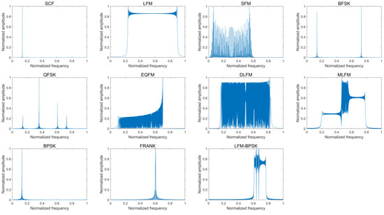
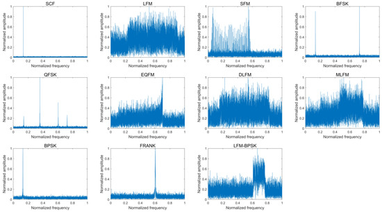
Figure 4. The frequency-domain amplitude spectra of eleven intra-pulse modulations of some radar emitter signal samples without noise (upper) and the according frequency-domain amplitude spectra when SNR is 0 dB (lower).

The SNR ranges from −12 dB to 0 dB with 1 dB increment. At each value of SNR, the number of samples for each type of intra-pulse modulation is 1200. That is, there are 171,600 samples in the dataset. In this paper, the proposed method aims to solve the semi-supervised classification problem, and we split the dataset with the following steps:

(1)

For the testing dataset, we select 400 samples for each type of intra-pulse modulation at each value of SNR from the original dataset.

(2)

For the labeled dataset, we select 30 samples for each type of intra-pulse modulation at each value of SNR from the original dataset.

(3)

The labeled dataset is divided into training dataset and validation dataset. For the training dataset, we select 15 samples for each type of intra-pulse modulation at each value of SNR from the labeled dataset. Similarly, for the validation dataset, we select 15 samples for each type of intra-pulse modulation at each value of SNR from the labeled dataset.

(4)

For the unlabeled dataset, we select 770 samples for each type of intra-pulse modulation at each value of SNR from the original dataset.

(5)

The unlabeled dataset is divided into two datasets: the 1th unlabeled dataset and the 2nd unlabeled dataset. For the 1th unlabeled dataset, we select 385 samples for each type of intra-pulse modulation at each value of SNR from the unlabeled dataset. Similarly, for the 2nd unlabeled dataset, we select 385 samples for each type of intra-pulse modulation at each value of SNR from the unlabeled dataset.

Note that there is no intersection of samples among the training dataset with 2145 samples, the validation dataset with 2145 samples, the 1th unlabeled dataset with 55,055 samples, the 2nd unlabeled dataset with 55,055 samples and the testing dataset with 57,200 samples. In addition, the number of each modulation at each value of SNR is the same in each dataset mentioned.

The reason why the number of samples in the validation dataset is larger and is the same as that of the training dataset is that a metric for judging the time when the weights are saved for the next training cycles is the accuracy of CNN for the validation dataset. Based on the experimental results in [19], if the number of samples in validation dataset is lower, the minimum graduation value for the accuracy will be higher, which will cause a larger difference in testing sessions. As the number of labeled samples is limited, splitting the labeled dataset in a half-to-half way would be suitable.

In addition, two unlabeled datasets, the 1-st unlabeled dataset and the 2nd unlabeled dataset, could reduce the uncertainty and increase the universality of the proposed method.

3.2. Parameters of MA-CNN

Due to the sampling frequency and the maximum of pulse width, based on Equation (8), the value of $k$ is calculated at 14, which represents that the point of FFT is 16,384. Therefore, the parameters of designed MA-CNN are shown in Table 2.

Table 2. The parameters of MA-CNN.

Input	Input Layer	Shape: 16384
Main Block 1	Convolutional Layer	Filters: 16 Kernel size: 16
	Max-Pooling	Stride: 6 Pooling_size: 6
	BatchNormalization	BatchNormalization
	Mixed Attention Block	MLP_1: Hidden layer 1: 16 nodes, activation: “ReLU” Hidden layer 2: 4 nodes, activation: “Sigmoid” MLP_2: Hidden layer 1: 32 nodes, activation: “ReLU” Hidden layer 2: 4 nodes, activation: “Sigmoid” Convolution Layer_1: Kernel size: 9, activation: “Sigmoid” Convolution Layer_2: Kernel size: 16, activation: “Sigmoid”
Main Block 2	Selective Convolutional Block	Filters: 32 First kernel size: 9 Second kernel size: 16 Nodes of first hidden layer in MLP: 8
	Max-Pooling	Stride: 6 Pooling_size: 6
	BatchNormalization	BatchNormalization
	Mixed Attention Block	MLP_1: Hidden layer 1: 32 nodes, activation: “ReLU” Hidden layer 2: 8 nodes, activation: “Sigmoid” MLP_2: Hidden layer 1: 64 nodes, activation: “ReLU” Hidden layer 2: 8 nodes, activation: “Sigmoid” Convolution Layer_1: Kernel size: 9, activation: “Sigmoid” Convolution Layer_2: Kernel size: 16, activation: “Sigmoid”
Main Block 3	Selective Convolutional Block	Filters: 64 First kernel size: 9 Second kernel size: 16 Nodes of first hidden layer in MLP: 8
	Max-Pooling	Stride: 6 Pooling_size: 6
	BatchNormalization	BatchNormalization
	Mixed Attention Block	MLP_1: Hidden layer 1: 64 nodes, activation: “ReLU” Hidden layer 2: 16 nodes, activation: “Sigmoid” MLP_2: Hidden layer 1: 128 nodes, activation: “ReLU” Hidden layer 2: 16 nodes, activation: “Sigmoid” Convolution Layer_1: Kernel size: 5, activation: “Sigmoid” Convolution Layer_2: Kernel size: 9, activation: “Sigmoid”
Main Block 4	Selective Convolutional Block	Filters: 128 First kernel size: 9 Second kernel size: 16 Nodes of first hidden layer in MLP: 8
	Max-Pooling	Stride: 6 Pooling_size: 6
	BatchNormalization	BatchNormalization
	Mixed Attention Block	MLP_1: Hidden layer 1: 128 nodes, activation: “ReLU” Hidden layer 2: 32 nodes, activation: “Sigmoid” MLP_2: Hidden layer 1: 256 nodes, activation: “ReLU” Hidden layer 2: 32 nodes, activation: “Sigmoid” Convolution Layer_1: Kernel size: 3, activation: “Sigmoid” Convolution Layer_2: Kernel size: 5, activation: “Sigmoid”
Full Connection Unit	Full Connection layer	Nodes: 512 Activation: “ReLU”
Output	Full Connection layer	Nodes: 11 Activation: “SoftMax”
Total Parameters: 1,033,195	Floating point operations: 2,063,221	Training time/10,000 iterations with 64 batch size: 410 s

The time usage for training the proposed MA-CNN based on different settings in Section 4 and Section 5 will be shown in Appendix A.8.

4. Experiments

To test the effectiveness of the proposed method, we apply it to the dataset and provide an extensive ablation study to tease apart the contribution of each of the proposed components. For convenience, we list the situations of the datasets that are used for training the MA-CNN in Table 3.

Table 3. The situations of the datasets that are used for training the MA-CNN.

Situation	Details
Situation Dataset1	Labeled dataset
Situation Dataset2	Labeled dataset + 1-st unlabeled dataset with true labels
Situation Dataset3	Labeled dataset + 2nd unlabeled dataset with true labels
Situation Dataset4	Labeled dataset + 1-st unlabeled dataset without true labels
Situation Dataset5	Labeled dataset + 2nd unlabeled dataset without true labels

The datasets in Situation Dataset 1, Situation Dataset 2 and Situation Dataset 3 are based on fully supervised conditions where the MA-CNN models trained by the datasets in these three situations can provide the standards of classification results with different numbers of labeled samples.

The samples in the Situation Dataset 4 and Situation Dataset 5 are in same distribution. These two situations are conducted to reduce the uncertainty and increase the universality of the proposed method. The datasets in the Situation Dataset 4 and Situation Dataset 5 are based on semi-supervised conditions, which will be used in our proposed methods.

In order to help readers understand the datasets used in different situations more intuitively, a visual diagram is shown in Figure 5, which describes the situations and their datasets visually.

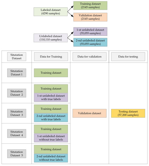
Figure 5. The datasets in different situations.

4.1. Implementation Details

In all experiments, we use the same structure of MA-CNN. Overall, the learning rate is set as 0.001 and the batch size as 64. The cross-entropy function is selected as the loss function. The optimization algorithm for MA-CNN is adaptive moment estimation (ADAM) [31]. There are 50 epochs in each training cycle. In addition, the initial weights of MA-CNN will be generated firstly and will be loaded at the start of each training cycle for the initialization. For each training cycle, the weights are saved based on the standard that the weights in this training cycle have the highest accuracy for the samples on validation dataset. Therefore, if the number of training cycle is, for example, 100, there will be 100 groups of weights. When all the training sessions are finished, we will select the best group of weights from all training cycles, which has the best accuracy for the validation dataset, to test the real performance.

The framework of our proposed method is shown in Algorithm 4.

Algorithm 4. The framework of our proposed method
Step 1	Train a MA-CNN model: $f$ with labeled samples $X$ and obtain the pre-trained CNN model: $f_{pre-trained}$.
Step 2	Set the value of training cycles: $T_{cycle}$. Set the value of $NUM$ and d in each round of training cycle.
Step 3	Generate pseudo labels for unlabeled samples by the latest well-trained MA-CNN: $f_{latest}$ and obtain the pseudo-labeled samples $U_{pseudo}$. Note that $f_{latest}$ refers to the latest trained MA-CNN. If it is the first time to generate pseudo labels, $f_{latest}$ will be $f_{pre-trained}$. Otherwise, $f_{latest}$ will be $f_{better}$ in Step 7.
Step 4	Based on the value of the current round of training cycle, select the $NUM$ samples with highest confidence in this round.
Step 5	Augment the selected pseudo-labeled samples $U_{pseudo}$ and normalize the results based on the value of d in this round.
Step 6	Train a better MA-CNN model: $f_{better}$ with the selected pseudo-labeled augmented samples and the labeled samples.
Step 7	Perform Step 3 to Step 7 until the training cycle reaches $T_{cycle}$.

In our proposed method, the value of $T_{cycle}$ is 100. The value of $NUM$ increases linearly, starting from 551 with 551 increments (in the last training cycle, the $NUM$ will be 55055). The value of d decreases linearly according to the value of $T_{cycle}$, starting from 1 to 0.

4.2. Experiments of Fully Supervised Baseline Methods

In this section, we analyze the classification performance of the model trained by the datasets in Situation Dataset 1, Situation Dataset 2 and Situation Dataset 3. Three fully supervision-based experiments with the datasets in Situation Dataset 1, Situation Dataset 2 and Situation Dataset 3, respectively, are carried out, and their classification results are shown in Table 4 and Table 5. The results in detail can be found in Table A1, Table A2 and Table A3 of Appendix A.1.

Table 4. The fully supervised classification accuracy for SNR with the datasets in Situation Dataset 1, Situation Dataset 2 and Situation Dataset 3.

SNR	−12	−11	−10	−9	−8	−7	−6	−5	−4	−3	−2	−1	0	Average
Situation Dataset 1	0.5625	0.5970	0.6370	0.6570	0.6820	0.7007	0.7370	0.7455	0.7730	0.7939	0.8073	0.8268	0.8193	0.7184
Situation Dataset 2	0.7884	0.8189	0.8650	0.8925	0.9130	0.9345	0.9548	0.9673	0.9823	0.9882	0.9923	0.9932	0.9957	0.9297
Situation Dataset 3	0.8127	0.8439	0.8750	0.8989	0.9173	0.9339	0.9577	0.9709	0.9848	0.9870	0.9907	0.9927	0.9948	0.9354

Table 5. The fully supervised classification accuracy for the classes with the datasets in Situation Dataset 1, Situation Dataset 2 and Situation Dataset 3.

	Situation	Situation Dataset 1	Situation Dataset 2	Situation Dataset 3
Class
SCF		0.9602	0.9990	0.9996
LFM		0.3217	0.8517	0.8175
SFM		0.9340	0.9879	0.9823
BFSK		0.8533	0.9954	0.9933
QFSK		0.9165	0.9969	0.9938
EQFM		0.7169	0.9829	0.9925
DLFM		0.5958	0.8769	0.9367
MLFM		0.3254	0.8113	0.8044
BPSK		0.9506	0.9990	0.9985
FRANK		0.9706	0.9996	0.9971
LFM-BPSK		0.3573	0.7258	0.7737
Average		0.7184	0.9297	0.9354

From the tables, we can find that the LFM signals, MLFM signals and LFM-BPSK signals are more difficult to be classified compared with other types of intra-pulse modulations. Besides, for these three types of signals, the classification accuracy of the model, which only uses a labeled dataset, is quite low. For other modulations, such as DLFM signals and EQFM signals, this model cannot classify them accurately when SNR is lower. In addition, there is a huge average accuracy gap between the model trained by labeled dataset and the model trained by both labeled dataset and unlabeled dataset with true labels. In summary, using only the labeled dataset with limited samples cannot bring about good classification results.

4.3. Experiments of the Proposed Method

In this section, we evaluate the accuracy of the proposed method trained by datasets in Situation Dataset 4 and Situation Dataset 5. The results can be seen in Table 6 and Table 7. The results of our proposed method in detail can be found from Table A4 and Table A5 of Appendix A.2.

Table 6. The semi-supervised classification accuracy of our proposed method for SNR with the datasets in Situation Dataset 4 and Situation Dataset 5.

SNR	−12	−11	−10	−9	−8	−7	−6	−5	−4	−3	−2	−1	0	Average
Situation Dataset 4	0.7398	0.7764	0.8136	0.8418	0.8595	0.8839	0.9030	0.9125	0.9225	0.9255	0.9318	0.9334	0.9309	0.8750
Situation Dataset 5	0.7305	0.7741	0.8168	0.8411	0.8650	0.8845	0.9030	0.9089	0.9186	0.9286	0.9407	0.9459	0.9350	0.8764

Table 7. The semi-supervised classification accuracy of our proposed method for the classes with the datasets in Situation Dataset 4 and Situation Dataset 5.

	Situation	Situation Dataset 4	Situation Dataset 5
Class
SCF		0.9935	0.9998
LFM		0.6925	0.5242
SFM		0.9781	0.9821
BFSK		0.9885	0.9713
QFSK		0.9938	0.9940
EQFM		0.9610	0.9798
DLFM		0.7444	0.7900
MLFM		0.6204	0.6487
BPSK		0.9965	0.9948
FRANK		0.9950	0.9948
LFM-BPSK		0.6610	0.7604
Average		0.8750	0.8764

Moreover, we provide the average classification accuracy of the model at each end of training cycle on the validation dataset in Figure 6.

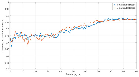
Figure 6. The average classification accuracy of the model at the end of each training cycle in the validation dataset.

Compared with the results in Section 4.2, we find that the classification accuracy of LFM signals, EQFM signals, DLFM signals, MLFM signals and LFM-BPSK signals improves a lot, especially for the LFM-BPSK signals.

Although the classification accuracy gap of our proposed method and the fully supervised method in classifying LFM signals, DLFM signals and MLFM signals still exists, for other modulations, the classification performance has little difference. In terms of average accuracy, the proposed method could improve the performance of classifying eleven intra-pulse modulations and could compete with the fully supervised situation-based model.

Figure 6 shows that the average accuracy of two experiments in the validation dataset at the first 30 training cycles is not stable and varies in range. However, the accuracy turns out to be stable and higher than the initial accuracy (the accuracy when training cycle is 0) as the training session goes, which shows the effectiveness of our proposed framework.

5. Discussion

Since our proposed method consists of selecting unlabeled samples and self-paced data augmentation, we study the effect of changing components in order to provide additional insight into what makes our method performant. Specifically, we measure the effects of changing the values of $T_{cycle}$ and $NUM$, removing the data augmentation and changing the strategy of self-paced data augmentation. The situations of the dataset are Situation Dataset 4 and Situation Dataset 5.

In addition, to verify the generality of the frameworks, specifically for generating pseudo labels, selecting unlabeled samples and self-paced data augmentation, we replace the proposed MA-CNN by 1-D SKCNN in [20], and the details can be found in Section 5.4. In Section 5.5, we provide some scenarios in which our method could be applied.

5.1. Ablation Study on the Value of $T_{cycle}$ and $NUM$

In this section, we will change the value of $T_{cycle}$ and $NUM$. Specifically, three experiments with different pairs of ($T_{cycle}$, $NUM$) are carried out. The value of d in self-paced data augmentation is still 1 to 0, decreasing linearly. The experimental results of ($T_{cycle}=26$, $NUM=2145$), ($T_{cycle}=50$, $NUM=1102$), ($T_{cycle}=100$, $NUM=551$) and ($T_{cycle}=200$, $NUM=276$) are shown in Table 8. The corresponding results in detail can be found from Table A6, Table A7, Table A8, Table A9, Table A10 and Table A11 of Appendix A.3.

Table 8. Semi-supervised classification results with the datasets with different values of $T_{cycle}$ and $NUM$.

SNR		−12	−11	−10	−9	−8	−7	−6	−5	−4	−3	−2	−1	0	Average
Situation Dataset 4	(26, 2145)	0.7309	0.7620	0.8052	0.8352	0.8530	0.8800	0.8977	0.9161	0.9200	0.9252	0.9257	0.9364	0.9255	0.8702
	(50, 1102)	0.7275	0.7607	0.7945	0.8357	0.8591	0.8718	0.8964	0.9157	0.9261	0.9334	0.9439	0.9491	0.9414	0.8735
	(100, 551)	0.7398	0.7764	0.8136	0.8418	0.8595	0.8839	0.9030	0.9125	0.9225	0.9255	0.9318	0.9334	0.9309	0.8750
	(200, 276)	0.7414	0.7773	0.8182	0.8470	0.8752	0.8982	0.9225	0.9282	0.9407	0.9489	0.9480	0.9523	0.9411	0.8876
Situation Dataset 5	(26, 2145)	0.7073	0.7439	0.7923	0.8186	0.8373	0.8652	0.8818	0.9043	0.9084	0.9123	0.9186	0.9270	0.9234	0.8570
	(50, 1102)	0.7086	0.7511	0.7809	0.8227	0.8509	0.8730	0.9057	0.9132	0.9314	0.9486	0.9559	0.9536	0.9550	0.8731
	(100, 551)	0.7305	0.7741	0.8168	0.8411	0.8650	0.8845	0.9030	0.9089	0.9186	0.9286	0.9407	0.9459	0.9350	0.8764
	(200, 276)	0.7436	0.7757	0.8209	0.8489	0.8666	0.8941	0.9109	0.9227	0.9307	0.9380	0.9425	0.9484	0.9407	0.8834

Combined with the results in Section 4.3, we find that when the value of $T_{cycle}$ increases, the average accuracy tends to increase. Although the experiments using the 2nd unlabeled dataset with ($T_{cycle}=26$, $NUM=2145$) and ($T_{cycle}=50$, $NUM=1102$) do not meet the tendency, the average accuracy of them is similarly lower than the other experimental group using the same datasets. In addition, although the tendency is that more training cycles can bring higher accuracy, the price is that more training cycles would cost more training time as they contain more iterations in total. The time usage for training the model based on these four pairs can be found in Appendix A.8.

As a result, it is important to balance the number of training cycles and the demand of classification accuracy. In this paper, the pair of ($T_{cycle}=100$, $NUM=551$) is more suitable.

5.2. Ablation Study on Data Augmentation

In this section, we will remove the self-paced data augmentation. Therefore, the unlabeled samples without any augmentation are used for training MA-CNN. Four experiments with pairs of ($T_{cycle}=26$, $NUM=2145$), ($T_{cycle}=50$, $NUM=1102$), ($T_{cycle}=100$, $NUM=551$) and ($T_{cycle}=200$, $NUM=276$) are carried out. The experimental results are shown in Table 9. The corresponding results in detail can be found from Table A12, Table A13, Table A14, Table A15, Table A16, Table A17, Table A18 and Table A19 of Appendix A.4.

Table 9. Semi-supervised classification results with the datasets without self-paced data augmentation.

SNR		−12	−11	−10	−9	−8	−7	−6	−5	−4	−3	−2	−1	0	Average
Situation Dataset 4	(26, 2145)	0.7005	0.7170	0.7409	0.7641	0.7880	0.8000	0.8114	0.8273	0.8318	0.8423	0.8475	0.8570	0.8552	0.7987
	(50, 1102)	0.7120	0.7243	0.7570	0.7745	0.7884	0.8009	0.8052	0.8211	0.8314	0.8382	0.8439	0.8482	0.8402	0.7989
	(100, 551)	0.7057	0.7286	0.7632	0.7825	0.7961	0.8180	0.8298	0.8420	0.8461	0.8539	0.8570	0.8652	0.8643	0.8117
	(200, 276)	0.7125	0.7266	0.7686	0.7905	0.8025	0.8332	0.8550	0.8664	0.8764	0.8907	0.8957	0.8995	0.8961	0.8318
Situation Dataset 5	(26, 2145)	0.7073	0.7252	0.7482	0.7668	0.7843	0.7959	0.8161	0.8218	0.8361	0.8393	0.8439	0.8543	0.8420	0.7986
	(50, 1102)	0.6836	0.7041	0.7336	0.7552	0.7800	0.7993	0.8177	0.8314	0.8384	0.8532	0.8614	0.8657	0.8593	0.7987
	(100, 551)	0.7105	0.7295	0.7723	0.7934	0.8145	0.8280	0.8427	0.8509	0.8652	0.8623	0.8659	0.8745	0.8702	0.8215
	(200, 276)	0.7075	0.7282	0.7686	0.7923	0.8134	0.8295	0.8561	0.8611	0.8755	0.8834	0.8880	0.8945	0.8907	0.8299

Combined with the tables in Section 4.3 and Section 5.1, we can find that pseudo-label learning without self-paced data augmentation can improve the classification accuracy compared with the classification result that only uses labeled datasets. However, the classification performance of these four models is all worse than the models in Section 5.1, where all the average accuracy of the models is at least 5% lower than that of the corresponding models in Section 5.1. Based on these experimental results, a conclusion can be drawn that the self-paced data augmentation in our proposed framework is necessary and effective, which can improve the performance of MA-CNN.

5.3. Ablation Study on the Strategy of Self-Paced Data Augmentation

In this section, we will change the strategy of self-paced data augmentation. Specifically, three experiments with the same pair of ($T_{cycle}=100$, $NUM=551$) are carried out. The differences between them are that, for the first experiment, the value of d in Equation (17) is constant at 1; for the second experiment, the value of d is constant at 0.5; and for the third experiment, the value of d decreases linearly, starting from 0.5 to 0. The experimental results are shown in Table 10. The corresponding results in detail can be found in Table A20, Table A21, Table A22, Table A23, Table A24 and Table A25 of Appendix A.5.

Table 10. Semi-supervised classification result with the datasets with different strategies of self-paced data augmentation.

SNR		−12	−11	−10	−9	−8	−7	−6	−5	−4	−3	−2	−1	0	Average
Situation Dataset 4	d = 1 constant	0.6511	0.6868	0.7198	0.7527	0.7655	0.7882	0.8243	0.8464	0.8723	0.8859	0.8930	0.9002	0.9050	0.8070
	d = 0.5 constant	0.6775	0.7155	0.7518	0.7768	0.8102	0.8398	0.8664	0.8936	0.9023	0.9084	0.9277	0.9330	0.9298	0.8410
	d = 0.5 decreasing linearly	0.6957	0.7275	0.7675	0.8048	0.8252	0.8595	0.8820	0.9109	0.9343	0.9459	0.9516	0.9561	0.9548	0.8628
Situation Dataset 5	d = 1 constant	0.6511	0.6768	0.7186	0.7420	0.7639	0.7864	0.8186	0.8386	0.8618	0.8757	0.8841	0.8882	0.8918	0.7998
	d = 0.5 constant	0.6934	0.7180	0.7489	0.7866	0.8091	0.8373	0.8686	0.8875	0.9057	0.9070	0.9184	0.9298	0.9243	0.8411
	d = 0.5 decreasing linearly	0.7132	0.7295	0.7761	0.8027	0.8293	0.8632	0.8852	0.9027	0.9186	0.9270	0.9334	0.9364	0.9370	0.8580

Combined with the tables in Section 4.3, we find the value of d influences the classification performance. Specifically, the strategy of the self-paced data augmentation that decreases the value of d according to the training cycles can improve the accuracy of the model. Moreover, in the case of this self-paced strategy, a higher initial value of d can lead a better result compared with a lower initial value of d.

5.4. Generality Study on Generating Pseudo Labels, Selecting Unlabeled Samples and Augmenting Self-Paced Data

In this section, we will evaluate the generality of generating pseudo labels, selecting unlabeled samples and augmenting self-paced data. Specifically, MA-CNN is replaced by an existing complicated 1-D SKCNN model in [20]. The structure of 1-D SKCNN can be found in Appendix A.6. Similarly, three fully supervision-based experiments with the datasets in Situation Dataset 1, Situation Dataset 2 and Situation Dataset 3, respectively, are carried out. Meanwhile, the semi-supervised classification is conducted based on the same strategies in Section 4.1. The classification results are shown in Table 11. The results in detail can be found in Table A26, Table A27, Table A28, Table A29 and Table A30 of Appendix A.7.

Table 11. The fully supervised classification accuracy for SNR with the datasets in Situation Dataset 1, Situation Dataset 2 and Situation Dataset 3 based on 1-D SKCNN.

SNR	−12	−11	−10	−9	−8	−7	−6	−5	−4	−3	−2	−1	0	Average
Situation Dataset 1	0.5927	0.6252	0.6532	0.6686	0.7055	0.7377	0.7564	0.7705	0.7936	0.8055	0.8182	0.8355	0.8207	0.7372
Situation Dataset 2	0.7955	0.8305	0.8707	0.8961	0.9157	0.9384	0.9586	0.9727	0.9811	0.9875	0.9916	0.9941	0.9927	0.9327
Situation Dataset 3	0.8093	0.8466	0.8750	0.9039	0.9182	0.9443	0.9589	0.9780	0.9866	0.9900	0.9939	0.9952	0.9970	0.9382
Situation Dataset 4	0.7559	0.7834	0.8200	0.8527	0.8770	0.9084	0.9275	0.9377	0.9495	0.9593	0.9636	0.9707	0.9675	0.8980
Situation Dataset 5	0.7434	0.7718	0.8236	0.8514	0.8818	0.9070	0.9330	0.9409	0.9539	0.9593	0.9645	0.9725	0.9675	0.8977

According to the table, we can find that although the classification results of 1-D SKCNN in semi-supervised conditions are better than those of MA-CNN, the tendency of accuracy based on 1-D SKCNN is same as that of MA-CNN, where the average accuracy rises by about 16% compared with the original 1-D SKCNN model that was trained only by the labeled samples. Focusing on the improvement of accuracy, we can draw the conclusion that the framework, specifically generating pseudo labels, selecting unlabeled samples and augmenting self-paced data, can be widely used in different structures of CNN models for semi-supervised intra-pulse modulation classification.

5.5. Application Scenarios

CNNs have been widely used in classification tasks, and the existing literature has proven the effectiveness of CNNs in intra-pulse modulation classification. However, the problem is that in the real environment, unlabeled samples are much greater than labeled samples, where the intra-pulse modulation classification tasks are semi-supervised. Through the experiments of MA-CNN and the extra experiments, which use 1-D SKCNN as the classification backbones, we can obtain the conclusion that generating pseudo labels, selecting unlabeled samples and augmenting self-paced data can increase the performance of the CNN model in a semi-supervised condition. At the same time, we also find that our framework requires more training cycles. Therefore, it would be essential to design the classification backbones in a light-weighted way if the computation resources are limited.

Currently, there are few studies focusing on semi-supervised classification of intra-pulse modulations of radar signals. Our method provides guidance for this type of classification.

6. Conclusions

In this paper, we focused on a more common semi-supervised instead of fully supervised situation and proposed a method to classify the intra-pulse modulation of radar emitter signals in the case where a very limited number of labeled samples and a large number of unlabeled samples are provided. Through the extensive experiments including the fully supervised baseline methods and other ablation study, we found that our proposed method, which combines generating pseudo labels, selecting high-confidence samples and augmenting self-paced data, can significantly improve the classification accuracy of eleven types of intra-pulse modulations of radar emitter signals in the semi-supervised situations. Additionally, the results of the generality study proved the generality of the components in our proposed method. Our proposed method in this paper could provide guidance for this type of semi-supervised classification.

In future work, we will attempt to focus on the extreme situation where the dataset only includes limited labeled samples. Furthermore, to reduce the training time and apply this framework into the real radar system is another problem for the future.

Appendix A.1. The Classification Results of the Experiments

Table A1. The fully supervised classification results with the datasets in Situation Dataset 1.

SNR	−12	−11	−10	−9	−8	−7	−6	−5	−4	−3	−2	−1	0	Average
SCF	0.9200	0.9375	0.9350	0.9700	0.9750	0.9650	0.9675	0.9875	0.9650	0.9650	0.9675	0.9675	0.9600	0.9602
LFM	0.2300	0.2125	0.2525	0.2425	0.2175	0.2650	0.2650	0.2925	0.3125	0.3775	0.4600	0.5325	0.5225	0.3217
SFM	0.7450	0.8475	0.9025	0.9275	0.9525	0.9550	0.9500	0.9600	0.9875	0.9775	0.9775	0.9775	0.9825	0.9340
BFSK	0.6900	0.7550	0.7900	0.8525	0.8650	0.8675	0.8725	0.8750	0.8900	0.9025	0.8825	0.9275	0.9225	0.8533
QFSK	0.7975	0.8700	0.9025	0.9275	0.9125	0.9275	0.9150	0.9050	0.9350	0.9575	0.9525	0.9625	0.9500	0.9165
EQFM	0.2900	0.3925	0.4825	0.5425	0.6450	0.7025	0.8100	0.8325	0.9025	0.9275	0.9250	0.9250	0.9425	0.7169
DLFM	0.2550	0.2550	0.3325	0.3425	0.4550	0.5375	0.6625	0.6750	0.7900	0.8125	0.8600	0.8950	0.8725	0.5958
MLFM	0.2100	0.1900	0.2125	0.2525	0.2675	0.2500	0.3325	0.3350	0.3475	0.4175	0.4400	0.4875	0.4875	0.3254
BPSK	0.9550	0.9475	0.9725	0.9625	0.9425	0.9400	0.9525	0.9550	0.9600	0.9200	0.9475	0.9525	0.9500	0.9506
FRANK	0.8575	0.9300	0.9500	0.9750	0.9875	0.9825	0.9900	0.9950	0.9775	0.9900	0.9975	0.9925	0.9925	0.9706
LFM-BPSK	0.2375	0.2300	0.2750	0.2325	0.2825	0.3150	0.3900	0.3875	0.4350	0.4850	0.4700	0.4750	0.4300	0.3573
Average	0.5625	0.5970	0.6370	0.6570	0.6820	0.7007	0.7370	0.7455	0.7730	0.7939	0.8073	0.8268	0.8193	0.7184

Table A1. The fully supervised classification results with the datasets in Situation Dataset 1.

SNR	−12	−11	−10	−9	−8	−7	−6	−5	−4	−3	−2	−1	0	Average
SCF	0.9200	0.9375	0.9350	0.9700	0.9750	0.9650	0.9675	0.9875	0.9650	0.9650	0.9675	0.9675	0.9600	0.9602
LFM	0.2300	0.2125	0.2525	0.2425	0.2175	0.2650	0.2650	0.2925	0.3125	0.3775	0.4600	0.5325	0.5225	0.3217
SFM	0.7450	0.8475	0.9025	0.9275	0.9525	0.9550	0.9500	0.9600	0.9875	0.9775	0.9775	0.9775	0.9825	0.9340
BFSK	0.6900	0.7550	0.7900	0.8525	0.8650	0.8675	0.8725	0.8750	0.8900	0.9025	0.8825	0.9275	0.9225	0.8533
QFSK	0.7975	0.8700	0.9025	0.9275	0.9125	0.9275	0.9150	0.9050	0.9350	0.9575	0.9525	0.9625	0.9500	0.9165
EQFM	0.2900	0.3925	0.4825	0.5425	0.6450	0.7025	0.8100	0.8325	0.9025	0.9275	0.9250	0.9250	0.9425	0.7169
DLFM	0.2550	0.2550	0.3325	0.3425	0.4550	0.5375	0.6625	0.6750	0.7900	0.8125	0.8600	0.8950	0.8725	0.5958
MLFM	0.2100	0.1900	0.2125	0.2525	0.2675	0.2500	0.3325	0.3350	0.3475	0.4175	0.4400	0.4875	0.4875	0.3254
BPSK	0.9550	0.9475	0.9725	0.9625	0.9425	0.9400	0.9525	0.9550	0.9600	0.9200	0.9475	0.9525	0.9500	0.9506
FRANK	0.8575	0.9300	0.9500	0.9750	0.9875	0.9825	0.9900	0.9950	0.9775	0.9900	0.9975	0.9925	0.9925	0.9706
LFM-BPSK	0.2375	0.2300	0.2750	0.2325	0.2825	0.3150	0.3900	0.3875	0.4350	0.4850	0.4700	0.4750	0.4300	0.3573
Average	0.5625	0.5970	0.6370	0.6570	0.6820	0.7007	0.7370	0.7455	0.7730	0.7939	0.8073	0.8268	0.8193	0.7184

Table A2. The fully supervised classification results with the datasets in Situation Dataset 2.

SNR	−12	−11	−10	−9	−8	−7	−6	−5	−4	−3	−2	−1	0	Average
SCF	0.9950	0.9925	1.0000	1.0000	1.0000	1.0000	1.0000	1.0000	1.0000	1.0000	1.0000	1.0000	1.0000	0.9990
LFM	0.4500	0.5725	0.6775	0.7725	0.8075	0.9000	0.9600	0.9700	0.9800	0.9900	0.9975	0.9975	0.9975	0.8517
SFM	0.9250	0.9700	0.9850	0.9925	0.9950	0.9975	0.9975	0.9950	0.9975	0.9975	0.9975	1.0000	0.9925	0.9879
BFSK	0.9800	0.9875	0.9950	0.9950	0.9975	0.9925	0.9975	0.9975	1.0000	0.9975	1.0000	1.0000	1.0000	0.9954
QFSK	0.9800	0.9875	0.9975	0.9975	1.0000	0.9975	1.0000	1.0000	1.0000	1.0000	1.0000	1.0000	1.0000	0.9969
EQFM	0.8825	0.9425	0.9775	0.9825	0.9950	0.9975	1.0000	1.0000	1.0000	1.0000	1.0000	1.0000	1.0000	0.9829
DLFM	0.5125	0.6000	0.7325	0.8375	0.9075	0.9300	0.9500	0.9600	0.9875	0.9900	0.9975	0.9950	1.0000	0.8769
MLFM	0.5200	0.5150	0.6400	0.6775	0.7400	0.8275	0.8800	0.9275	0.9475	0.9675	0.9675	0.9650	0.9725	0.8113
BPSK	0.9925	0.9975	1.0000	0.9975	1.0000	1.0000	1.0000	1.0000	1.0000	1.0000	1.0000	1.0000	1.0000	0.9990
FRANK	0.9950	1.0000	1.0000	1.0000	1.0000	1.0000	1.0000	1.0000	1.0000	1.0000	1.0000	1.0000	1.0000	0.9996
LFM-BPSK	0.4400	0.4425	0.5100	0.5650	0.6000	0.6375	0.7175	0.7900	0.8925	0.9275	0.9550	0.9675	0.9900	0.7258
Average	0.7884	0.8189	0.8650	0.8925	0.9130	0.9345	0.9548	0.9673	0.9823	0.9882	0.9923	0.9932	0.9957	0.9297

Table A2. The fully supervised classification results with the datasets in Situation Dataset 2.

SNR	−12	−11	−10	−9	−8	−7	−6	−5	−4	−3	−2	−1	0	Average
SCF	0.9950	0.9925	1.0000	1.0000	1.0000	1.0000	1.0000	1.0000	1.0000	1.0000	1.0000	1.0000	1.0000	0.9990
LFM	0.4500	0.5725	0.6775	0.7725	0.8075	0.9000	0.9600	0.9700	0.9800	0.9900	0.9975	0.9975	0.9975	0.8517
SFM	0.9250	0.9700	0.9850	0.9925	0.9950	0.9975	0.9975	0.9950	0.9975	0.9975	0.9975	1.0000	0.9925	0.9879
BFSK	0.9800	0.9875	0.9950	0.9950	0.9975	0.9925	0.9975	0.9975	1.0000	0.9975	1.0000	1.0000	1.0000	0.9954
QFSK	0.9800	0.9875	0.9975	0.9975	1.0000	0.9975	1.0000	1.0000	1.0000	1.0000	1.0000	1.0000	1.0000	0.9969
EQFM	0.8825	0.9425	0.9775	0.9825	0.9950	0.9975	1.0000	1.0000	1.0000	1.0000	1.0000	1.0000	1.0000	0.9829
DLFM	0.5125	0.6000	0.7325	0.8375	0.9075	0.9300	0.9500	0.9600	0.9875	0.9900	0.9975	0.9950	1.0000	0.8769
MLFM	0.5200	0.5150	0.6400	0.6775	0.7400	0.8275	0.8800	0.9275	0.9475	0.9675	0.9675	0.9650	0.9725	0.8113
BPSK	0.9925	0.9975	1.0000	0.9975	1.0000	1.0000	1.0000	1.0000	1.0000	1.0000	1.0000	1.0000	1.0000	0.9990
FRANK	0.9950	1.0000	1.0000	1.0000	1.0000	1.0000	1.0000	1.0000	1.0000	1.0000	1.0000	1.0000	1.0000	0.9996
LFM-BPSK	0.4400	0.4425	0.5100	0.5650	0.6000	0.6375	0.7175	0.7900	0.8925	0.9275	0.9550	0.9675	0.9900	0.7258
Average	0.7884	0.8189	0.8650	0.8925	0.9130	0.9345	0.9548	0.9673	0.9823	0.9882	0.9923	0.9932	0.9957	0.9297

Table A3. The fully supervised classification results with the datasets in Situation Dataset 3.

SNR	−12	−11	−10	−9	−8	−7	−6	−5	−4	−3	−2	−1	0	Average
SCF	0.9975	0.9975	1.0000	1.0000	1.0000	1.0000	1.0000	1.0000	1.0000	1.0000	1.0000	1.0000	1.0000	0.9996
LFM	0.4425	0.5575	0.6400	0.7200	0.7525	0.7975	0.8750	0.9300	0.9600	0.9775	0.9825	0.9975	0.9950	0.8175
SFM	0.9150	0.9475	0.9825	0.9850	0.9975	0.9900	0.9900	0.9925	1.0000	0.9925	0.9950	0.9950	0.9875	0.9823
BFSK	0.9750	0.9800	0.9900	0.9950	0.9950	0.9950	0.9925	0.9975	1.0000	1.0000	1.0000	0.9975	0.9950	0.9933
QFSK	0.9675	0.9800	0.9950	0.9925	0.9950	0.9975	0.9975	1.0000	0.9975	0.9975	1.0000	1.0000	1.0000	0.9938
EQFM	0.9250	0.9850	0.9950	0.9975	1.0000	1.0000	1.0000	1.0000	1.0000	1.0000	1.0000	1.0000	1.0000	0.9925
DLFM	0.7125	0.7900	0.8700	0.9225	0.9550	0.9700	0.9850	0.9875	1.0000	0.9950	0.9925	0.9975	1.0000	0.9367
MLFM	0.5600	0.5775	0.6250	0.6600	0.7325	0.7900	0.8625	0.9000	0.9150	0.9350	0.9625	0.9575	0.9800	0.8044
BPSK	0.9850	0.9975	0.9975	1.0000	1.0000	1.0000	1.0000	1.0000	1.0000	1.0000	1.0000	1.0000	1.0000	0.9985
FRANK	0.9950	0.9975	1.0000	0.9975	1.0000	1.0000	1.0000	1.0000	1.0000	0.9975	0.9925	0.9950	0.9875	0.9971
LFM-BPSK	0.4650	0.4725	0.5300	0.6175	0.6625	0.7325	0.8325	0.8725	0.9600	0.9625	0.9725	0.9800	0.9975	0.7737
Average	0.8127	0.8439	0.8750	0.8989	0.9173	0.9339	0.9577	0.9709	0.9848	0.9870	0.9907	0.9927	0.9948	0.9354

Table A3. The fully supervised classification results with the datasets in Situation Dataset 3.

SNR	−12	−11	−10	−9	−8	−7	−6	−5	−4	−3	−2	−1	0	Average
SCF	0.9975	0.9975	1.0000	1.0000	1.0000	1.0000	1.0000	1.0000	1.0000	1.0000	1.0000	1.0000	1.0000	0.9996
LFM	0.4425	0.5575	0.6400	0.7200	0.7525	0.7975	0.8750	0.9300	0.9600	0.9775	0.9825	0.9975	0.9950	0.8175
SFM	0.9150	0.9475	0.9825	0.9850	0.9975	0.9900	0.9900	0.9925	1.0000	0.9925	0.9950	0.9950	0.9875	0.9823
BFSK	0.9750	0.9800	0.9900	0.9950	0.9950	0.9950	0.9925	0.9975	1.0000	1.0000	1.0000	0.9975	0.9950	0.9933
QFSK	0.9675	0.9800	0.9950	0.9925	0.9950	0.9975	0.9975	1.0000	0.9975	0.9975	1.0000	1.0000	1.0000	0.9938
EQFM	0.9250	0.9850	0.9950	0.9975	1.0000	1.0000	1.0000	1.0000	1.0000	1.0000	1.0000	1.0000	1.0000	0.9925
DLFM	0.7125	0.7900	0.8700	0.9225	0.9550	0.9700	0.9850	0.9875	1.0000	0.9950	0.9925	0.9975	1.0000	0.9367
MLFM	0.5600	0.5775	0.6250	0.6600	0.7325	0.7900	0.8625	0.9000	0.9150	0.9350	0.9625	0.9575	0.9800	0.8044
BPSK	0.9850	0.9975	0.9975	1.0000	1.0000	1.0000	1.0000	1.0000	1.0000	1.0000	1.0000	1.0000	1.0000	0.9985
FRANK	0.9950	0.9975	1.0000	0.9975	1.0000	1.0000	1.0000	1.0000	1.0000	0.9975	0.9925	0.9950	0.9875	0.9971
LFM-BPSK	0.4650	0.4725	0.5300	0.6175	0.6625	0.7325	0.8325	0.8725	0.9600	0.9625	0.9725	0.9800	0.9975	0.7737
Average	0.8127	0.8439	0.8750	0.8989	0.9173	0.9339	0.9577	0.9709	0.9848	0.9870	0.9907	0.9927	0.9948	0.9354

Appendix A.2. The Classification Results of the Experiments

Table A4. Semi-supervised classification results of our proposed method with the datasets in Situation Dataset 4.

SNR	−12	−11	−10	−9	−8	−7	−6	−5	−4	−3	−2	−1	0	Average
SCF	0.9975	0.9900	0.9975	0.9975	0.9900	0.9950	0.9975	0.9925	0.9925	0.9900	0.9925	0.9925	0.9900	0.9935
LFM	0.4075	0.5025	0.5450	0.6300	0.6300	0.6875	0.7675	0.7900	0.7700	0.7950	0.8050	0.8350	0.8375	0.6925
SFM	0.8600	0.9375	0.9700	0.9800	0.9875	0.9975	0.9925	0.9950	1.0000	1.0000	1.0000	0.9975	0.9975	0.9781
BFSK	0.9675	0.9750	0.9700	0.9850	0.9875	0.9950	0.9975	0.9950	0.9975	0.9950	0.9950	0.9925	0.9975	0.9885
QFSK	0.9825	0.9750	0.9900	0.9850	0.9950	0.9925	1.0000	1.0000	1.0000	1.0000	1.0000	1.0000	1.0000	0.9938
EQFM	0.7850	0.8675	0.9300	0.9500	0.9925	0.9775	0.9925	1.0000	0.9975	1.0000	1.0000	1.0000	1.0000	0.9610
DLFM	0.3900	0.4225	0.5500	0.6000	0.6975	0.7875	0.8325	0.8650	0.8975	0.8850	0.9325	0.9175	0.9000	0.7444
MLFM	0.5000	0.5250	0.6175	0.6675	0.6125	0.6600	0.6475	0.6325	0.6650	0.6425	0.6450	0.6525	0.5975	0.6204
BPSK	0.9925	0.9900	0.9925	0.9950	0.9950	0.9975	1.0000	0.9975	1.0000	1.0000	1.0000	1.0000	0.9950	0.9965
FRANK	0.9825	0.9950	0.9975	1.0000	0.9950	1.0000	0.9975	1.0000	0.9950	0.9975	0.9925	0.9975	0.9850	0.9950
LFM-BPSK	0.2725	0.3600	0.3900	0.4700	0.5725	0.6325	0.7075	0.7700	0.8325	0.8750	0.8875	0.8825	0.9400	0.6610
Average	0.7398	0.7764	0.8136	0.8418	0.8595	0.8839	0.9030	0.9125	0.9225	0.9255	0.9318	0.9334	0.9309	0.8750

Table A4. Semi-supervised classification results of our proposed method with the datasets in Situation Dataset 4.

SNR	−12	−11	−10	−9	−8	−7	−6	−5	−4	−3	−2	−1	0	Average
SCF	0.9975	0.9900	0.9975	0.9975	0.9900	0.9950	0.9975	0.9925	0.9925	0.9900	0.9925	0.9925	0.9900	0.9935
LFM	0.4075	0.5025	0.5450	0.6300	0.6300	0.6875	0.7675	0.7900	0.7700	0.7950	0.8050	0.8350	0.8375	0.6925
SFM	0.8600	0.9375	0.9700	0.9800	0.9875	0.9975	0.9925	0.9950	1.0000	1.0000	1.0000	0.9975	0.9975	0.9781
BFSK	0.9675	0.9750	0.9700	0.9850	0.9875	0.9950	0.9975	0.9950	0.9975	0.9950	0.9950	0.9925	0.9975	0.9885
QFSK	0.9825	0.9750	0.9900	0.9850	0.9950	0.9925	1.0000	1.0000	1.0000	1.0000	1.0000	1.0000	1.0000	0.9938
EQFM	0.7850	0.8675	0.9300	0.9500	0.9925	0.9775	0.9925	1.0000	0.9975	1.0000	1.0000	1.0000	1.0000	0.9610
DLFM	0.3900	0.4225	0.5500	0.6000	0.6975	0.7875	0.8325	0.8650	0.8975	0.8850	0.9325	0.9175	0.9000	0.7444
MLFM	0.5000	0.5250	0.6175	0.6675	0.6125	0.6600	0.6475	0.6325	0.6650	0.6425	0.6450	0.6525	0.5975	0.6204
BPSK	0.9925	0.9900	0.9925	0.9950	0.9950	0.9975	1.0000	0.9975	1.0000	1.0000	1.0000	1.0000	0.9950	0.9965
FRANK	0.9825	0.9950	0.9975	1.0000	0.9950	1.0000	0.9975	1.0000	0.9950	0.9975	0.9925	0.9975	0.9850	0.9950
LFM-BPSK	0.2725	0.3600	0.3900	0.4700	0.5725	0.6325	0.7075	0.7700	0.8325	0.8750	0.8875	0.8825	0.9400	0.6610
Average	0.7398	0.7764	0.8136	0.8418	0.8595	0.8839	0.9030	0.9125	0.9225	0.9255	0.9318	0.9334	0.9309	0.8750

Table A5. Semi-supervised classification results of our proposed method with the datasets in Situation Dataset 5.

SNR	−12	−11	−10	−9	−8	−7	−6	−5	−4	−3	−2	−1	0	Average
SCF	1.0000	0.9975	1.0000	1.0000	1.0000	1.0000	1.0000	1.0000	1.0000	1.0000	1.0000	1.0000	1.0000	0.9998
LFM	0.2975	0.3475	0.3500	0.3775	0.4400	0.4975	0.5075	0.5350	0.6025	0.6775	0.6975	0.7475	0.7375	0.5242
SFM	0.9075	0.9525	0.9725	0.9850	0.9900	0.9975	0.9900	0.9900	1.0000	0.9950	0.9975	0.9975	0.9925	0.9821
BFSK	0.8400	0.9400	0.9550	0.9750	0.9775	0.9875	0.9925	0.9850	1.0000	0.9950	0.9900	0.9975	0.9925	0.9713
QFSK	0.9750	0.9850	1.0000	0.9925	0.9950	0.9900	0.9950	0.9950	0.9975	0.9975	1.0000	1.0000	1.0000	0.9940
EQFM	0.8550	0.9475	0.9650	0.9850	0.9975	0.9875	1.0000	1.0000	1.0000	1.0000	1.0000	1.0000	1.0000	0.9798
DLFM	0.3600	0.4500	0.5900	0.6625	0.7625	0.8275	0.8950	0.9175	0.9375	0.9550	0.9800	0.9700	0.9625	0.7900
MLFM	0.5275	0.5125	0.6075	0.6575	0.6175	0.6750	0.7275	0.6900	0.6575	0.6650	0.7250	0.7325	0.6375	0.6487
BPSK	0.9750	0.9825	0.9900	0.9875	1.0000	0.9975	1.0000	1.0000	1.0000	1.0000	1.0000	1.0000	1.0000	0.9948
FRANK	0.9700	0.9875	0.9975	0.9975	0.9975	1.0000	1.0000	1.0000	1.0000	0.9950	0.9975	0.9975	0.9925	0.9948
LFM-BPSK	0.3275	0.4125	0.5575	0.6325	0.7375	0.7700	0.8250	0.8850	0.9100	0.9350	0.9600	0.9625	0.9700	0.7604
Average	0.7305	0.7741	0.8168	0.8411	0.8650	0.8845	0.9030	0.9089	0.9186	0.9286	0.9407	0.9459	0.9350	0.8764

Table A5. Semi-supervised classification results of our proposed method with the datasets in Situation Dataset 5.

SNR	−12	−11	−10	−9	−8	−7	−6	−5	−4	−3	−2	−1	0	Average
SCF	1.0000	0.9975	1.0000	1.0000	1.0000	1.0000	1.0000	1.0000	1.0000	1.0000	1.0000	1.0000	1.0000	0.9998
LFM	0.2975	0.3475	0.3500	0.3775	0.4400	0.4975	0.5075	0.5350	0.6025	0.6775	0.6975	0.7475	0.7375	0.5242
SFM	0.9075	0.9525	0.9725	0.9850	0.9900	0.9975	0.9900	0.9900	1.0000	0.9950	0.9975	0.9975	0.9925	0.9821
BFSK	0.8400	0.9400	0.9550	0.9750	0.9775	0.9875	0.9925	0.9850	1.0000	0.9950	0.9900	0.9975	0.9925	0.9713
QFSK	0.9750	0.9850	1.0000	0.9925	0.9950	0.9900	0.9950	0.9950	0.9975	0.9975	1.0000	1.0000	1.0000	0.9940
EQFM	0.8550	0.9475	0.9650	0.9850	0.9975	0.9875	1.0000	1.0000	1.0000	1.0000	1.0000	1.0000	1.0000	0.9798
DLFM	0.3600	0.4500	0.5900	0.6625	0.7625	0.8275	0.8950	0.9175	0.9375	0.9550	0.9800	0.9700	0.9625	0.7900
MLFM	0.5275	0.5125	0.6075	0.6575	0.6175	0.6750	0.7275	0.6900	0.6575	0.6650	0.7250	0.7325	0.6375	0.6487
BPSK	0.9750	0.9825	0.9900	0.9875	1.0000	0.9975	1.0000	1.0000	1.0000	1.0000	1.0000	1.0000	1.0000	0.9948
FRANK	0.9700	0.9875	0.9975	0.9975	0.9975	1.0000	1.0000	1.0000	1.0000	0.9950	0.9975	0.9975	0.9925	0.9948
LFM-BPSK	0.3275	0.4125	0.5575	0.6325	0.7375	0.7700	0.8250	0.8850	0.9100	0.9350	0.9600	0.9625	0.9700	0.7604
Average	0.7305	0.7741	0.8168	0.8411	0.8650	0.8845	0.9030	0.9089	0.9186	0.9286	0.9407	0.9459	0.9350	0.8764

Appendix A.3. The Classification Results of the Experiments

Table A6. Semi-supervised classification results with the datasets in Situation Dataset 4 ($T_{cycle}=26$, $NUM=2145$).

SNR	−12	−11	−10	−9	−8	−7	−6	−5	−4	−3	−2	−1	0	Average
SCF	0.9750	0.9675	0.9625	0.9625	0.9650	0.9750	0.9675	0.9800	0.9700	0.9550	0.9525	0.9625	0.9500	0.9650
LFM	0.4725	0.4925	0.5675	0.6625	0.7075	0.7325	0.7600	0.7825	0.7675	0.8000	0.7875	0.8300	0.7975	0.7046
SFM	0.8925	0.9400	0.9700	0.9775	0.9875	0.9900	0.9850	0.9900	0.9950	0.9975	0.9975	0.9950	0.9925	0.9777
BFSK	0.9425	0.9675	0.9925	0.9750	0.9900	0.9875	0.9950	0.9950	0.9950	0.9950	0.9975	0.9950	0.9950	0.9863
QFSK	0.9500	0.9750	0.9850	0.9775	0.9875	0.9925	0.9975	0.9950	1.0000	1.0000	0.9975	1.0000	1.0000	0.9890
EQFM	0.8800	0.9525	0.9625	0.9850	1.0000	0.9975	1.0000	1.0000	1.0000	1.0000	1.0000	1.0000	1.0000	0.9829
DLFM	0.3350	0.3775	0.5600	0.6200	0.6975	0.8100	0.8850	0.9025	0.9150	0.9100	0.9250	0.9325	0.9125	0.7525
MLFM	0.4250	0.4775	0.5575	0.6400	0.5800	0.6450	0.6475	0.6975	0.6525	0.6625	0.6500	0.6825	0.6175	0.6104
BPSK	0.9325	0.9525	0.9500	0.9600	0.9775	0.9675	0.9875	0.9875	0.9875	0.9800	0.9850	0.9825	0.9700	0.9708
FRANK	0.9675	0.9825	0.9825	0.9975	0.9975	0.9950	0.9950	0.9975	0.9975	0.9950	0.9975	0.9975	0.9975	0.9923
LFM-BPSK	0.2675	0.2975	0.3675	0.4300	0.4925	0.5875	0.6550	0.7500	0.8400	0.8825	0.8925	0.9225	0.9475	0.6410
Average	0.7309	0.7620	0.8052	0.8352	0.8530	0.8800	0.8977	0.9161	0.9200	0.9252	0.9257	0.9364	0.9255	0.8702

Table A6. Semi-supervised classification results with the datasets in Situation Dataset 4 ($T_{cycle}=26$, $NUM=2145$).

SNR	−12	−11	−10	−9	−8	−7	−6	−5	−4	−3	−2	−1	0	Average
SCF	0.9750	0.9675	0.9625	0.9625	0.9650	0.9750	0.9675	0.9800	0.9700	0.9550	0.9525	0.9625	0.9500	0.9650
LFM	0.4725	0.4925	0.5675	0.6625	0.7075	0.7325	0.7600	0.7825	0.7675	0.8000	0.7875	0.8300	0.7975	0.7046
SFM	0.8925	0.9400	0.9700	0.9775	0.9875	0.9900	0.9850	0.9900	0.9950	0.9975	0.9975	0.9950	0.9925	0.9777
BFSK	0.9425	0.9675	0.9925	0.9750	0.9900	0.9875	0.9950	0.9950	0.9950	0.9950	0.9975	0.9950	0.9950	0.9863
QFSK	0.9500	0.9750	0.9850	0.9775	0.9875	0.9925	0.9975	0.9950	1.0000	1.0000	0.9975	1.0000	1.0000	0.9890
EQFM	0.8800	0.9525	0.9625	0.9850	1.0000	0.9975	1.0000	1.0000	1.0000	1.0000	1.0000	1.0000	1.0000	0.9829
DLFM	0.3350	0.3775	0.5600	0.6200	0.6975	0.8100	0.8850	0.9025	0.9150	0.9100	0.9250	0.9325	0.9125	0.7525
MLFM	0.4250	0.4775	0.5575	0.6400	0.5800	0.6450	0.6475	0.6975	0.6525	0.6625	0.6500	0.6825	0.6175	0.6104
BPSK	0.9325	0.9525	0.9500	0.9600	0.9775	0.9675	0.9875	0.9875	0.9875	0.9800	0.9850	0.9825	0.9700	0.9708
FRANK	0.9675	0.9825	0.9825	0.9975	0.9975	0.9950	0.9950	0.9975	0.9975	0.9950	0.9975	0.9975	0.9975	0.9923
LFM-BPSK	0.2675	0.2975	0.3675	0.4300	0.4925	0.5875	0.6550	0.7500	0.8400	0.8825	0.8925	0.9225	0.9475	0.6410
Average	0.7309	0.7620	0.8052	0.8352	0.8530	0.8800	0.8977	0.9161	0.9200	0.9252	0.9257	0.9364	0.9255	0.8702

Table A7. Semi-supervised classification results with the datasets in Situation Dataset 5 ($T_{cycle}=26$, $NUM=2145$).

SNR	−12	−11	−10	−9	−8	−7	−6	−5	−4	−3	−2	−1	0	Average
SCF	0.9750	0.9650	0.9675	0.9575	0.9600	0.9600	0.9700	0.9875	0.9625	0.9425	0.9575	0.9650	0.9500	0.9631
LFM	0.3650	0.4200	0.4350	0.4550	0.5300	0.5425	0.6075	0.6525	0.7100	0.7500	0.7725	0.8100	0.8225	0.6056
SFM	0.8400	0.9050	0.9450	0.9550	0.9750	0.9900	0.9775	0.9900	1.0000	0.9925	0.9950	0.9975	0.9850	0.9652
BFSK	0.9300	0.9225	0.9200	0.9525	0.9625	0.9700	0.9800	0.9775	0.9875	0.9850	0.9800	0.9875	0.9825	0.9644
QFSK	0.8950	0.9150	0.9500	0.9300	0.9550	0.9800	0.9850	0.9975	0.9975	1.0000	0.9975	1.0000	1.0000	0.9694
EQFM	0.8700	0.9400	0.9575	0.9775	0.9950	0.9775	0.9950	0.9950	1.0000	0.9975	0.9975	0.9975	1.0000	0.9769
DLFM	0.2925	0.3300	0.5450	0.6500	0.6925	0.7550	0.8375	0.8775	0.9025	0.8975	0.9150	0.9350	0.9325	0.7356
MLFM	0.4300	0.4650	0.5600	0.5850	0.5250	0.6450	0.6050	0.6675	0.6100	0.6375	0.6625	0.6550	0.6100	0.5890
BPSK	0.9500	0.9600	0.9550	0.9725	0.9625	0.9700	0.9875	0.9850	0.9825	0.9925	0.9950	0.9825	0.9875	0.9756
FRANK	0.9400	0.9750	0.9950	0.9875	0.9925	0.9900	0.9850	0.9900	0.9850	0.9725	0.9675	0.9550	0.9750	0.9777
LFM-BPSK	0.2925	0.3850	0.4850	0.5825	0.6600	0.7375	0.7700	0.8275	0.8550	0.8675	0.8650	0.9125	0.9125	0.7040
Average	0.7073	0.7439	0.7923	0.8186	0.8373	0.8652	0.8818	0.9043	0.9084	0.9123	0.9186	0.9270	0.9234	0.8570

Table A7. Semi-supervised classification results with the datasets in Situation Dataset 5 ($T_{cycle}=26$, $NUM=2145$).

SNR	−12	−11	−10	−9	−8	−7	−6	−5	−4	−3	−2	−1	0	Average
SCF	0.9750	0.9650	0.9675	0.9575	0.9600	0.9600	0.9700	0.9875	0.9625	0.9425	0.9575	0.9650	0.9500	0.9631
LFM	0.3650	0.4200	0.4350	0.4550	0.5300	0.5425	0.6075	0.6525	0.7100	0.7500	0.7725	0.8100	0.8225	0.6056
SFM	0.8400	0.9050	0.9450	0.9550	0.9750	0.9900	0.9775	0.9900	1.0000	0.9925	0.9950	0.9975	0.9850	0.9652
BFSK	0.9300	0.9225	0.9200	0.9525	0.9625	0.9700	0.9800	0.9775	0.9875	0.9850	0.9800	0.9875	0.9825	0.9644
QFSK	0.8950	0.9150	0.9500	0.9300	0.9550	0.9800	0.9850	0.9975	0.9975	1.0000	0.9975	1.0000	1.0000	0.9694
EQFM	0.8700	0.9400	0.9575	0.9775	0.9950	0.9775	0.9950	0.9950	1.0000	0.9975	0.9975	0.9975	1.0000	0.9769
DLFM	0.2925	0.3300	0.5450	0.6500	0.6925	0.7550	0.8375	0.8775	0.9025	0.8975	0.9150	0.9350	0.9325	0.7356
MLFM	0.4300	0.4650	0.5600	0.5850	0.5250	0.6450	0.6050	0.6675	0.6100	0.6375	0.6625	0.6550	0.6100	0.5890
BPSK	0.9500	0.9600	0.9550	0.9725	0.9625	0.9700	0.9875	0.9850	0.9825	0.9925	0.9950	0.9825	0.9875	0.9756
FRANK	0.9400	0.9750	0.9950	0.9875	0.9925	0.9900	0.9850	0.9900	0.9850	0.9725	0.9675	0.9550	0.9750	0.9777
LFM-BPSK	0.2925	0.3850	0.4850	0.5825	0.6600	0.7375	0.7700	0.8275	0.8550	0.8675	0.8650	0.9125	0.9125	0.7040
Average	0.7073	0.7439	0.7923	0.8186	0.8373	0.8652	0.8818	0.9043	0.9084	0.9123	0.9186	0.9270	0.9234	0.8570

Table A8. Semi-supervised classification results with the datasets in Situation Dataset 4 ($T_{cycle}=50$, $NUM=1102$).

SNR	−12	−11	−10	−9	−8	−7	−6	−5	−4	−3	−2	−1	0	Average
SCF	0.9975	1.0000	0.9975	1.0000	0.9975	1.0000	0.9950	1.0000	0.9950	0.9800	0.9750	0.9925	0.9750	0.9927
LFM	0.3250	0.3600	0.3850	0.4875	0.5575	0.5400	0.6200	0.6800	0.6750	0.7325	0.7375	0.7725	0.7650	0.5875
SFM	0.9175	0.9375	0.9775	0.9900	0.9925	0.9975	0.9950	0.9950	1.0000	1.0000	1.0000	0.9975	0.9950	0.9842
BFSK	0.9725	0.9700	0.9850	0.9825	0.9950	0.9925	0.9850	0.9950	0.9975	0.9975	0.9950	0.9925	0.9900	0.9885
QFSK	0.9000	0.9250	0.9525	0.9775	0.9850	0.9925	0.9975	0.9975	1.0000	1.0000	1.0000	1.0000	1.0000	0.9790
EQFM	0.9175	0.9700	0.9725	0.9925	0.9975	0.9975	0.9950	1.0000	1.0000	1.0000	1.0000	1.0000	1.0000	0.9879
DLFM	0.3300	0.4000	0.5250	0.5925	0.6900	0.7275	0.7800	0.8100	0.8875	0.8900	0.9225	0.9525	0.9500	0.7275
MLFM	0.4475	0.4975	0.5775	0.6750	0.7025	0.7125	0.7625	0.7850	0.8050	0.8075	0.8650	0.8575	0.7900	0.7142
BPSK	0.9200	0.9175	0.9375	0.9525	0.9425	0.9500	0.9650	0.9725	0.9575	0.9500	0.9500	0.9350	0.9250	0.9442
FRANK	0.9750	0.9975	0.9925	0.9975	0.9950	1.0000	1.0000	1.0000	1.0000	0.9975	1.0000	1.0000	1.0000	0.9965
LFM-BPSK	0.3000	0.3925	0.4375	0.5450	0.5950	0.6800	0.7650	0.8375	0.8700	0.9125	0.9375	0.9400	0.9650	0.7060
Average	0.7275	0.7607	0.7945	0.8357	0.8591	0.8718	0.8964	0.9157	0.9261	0.9334	0.9439	0.9491	0.9414	0.8735

Table A8. Semi-supervised classification results with the datasets in Situation Dataset 4 ($T_{cycle}=50$, $NUM=1102$).

SNR	−12	−11	−10	−9	−8	−7	−6	−5	−4	−3	−2	−1	0	Average
SCF	0.9975	1.0000	0.9975	1.0000	0.9975	1.0000	0.9950	1.0000	0.9950	0.9800	0.9750	0.9925	0.9750	0.9927
LFM	0.3250	0.3600	0.3850	0.4875	0.5575	0.5400	0.6200	0.6800	0.6750	0.7325	0.7375	0.7725	0.7650	0.5875
SFM	0.9175	0.9375	0.9775	0.9900	0.9925	0.9975	0.9950	0.9950	1.0000	1.0000	1.0000	0.9975	0.9950	0.9842
BFSK	0.9725	0.9700	0.9850	0.9825	0.9950	0.9925	0.9850	0.9950	0.9975	0.9975	0.9950	0.9925	0.9900	0.9885
QFSK	0.9000	0.9250	0.9525	0.9775	0.9850	0.9925	0.9975	0.9975	1.0000	1.0000	1.0000	1.0000	1.0000	0.9790
EQFM	0.9175	0.9700	0.9725	0.9925	0.9975	0.9975	0.9950	1.0000	1.0000	1.0000	1.0000	1.0000	1.0000	0.9879
DLFM	0.3300	0.4000	0.5250	0.5925	0.6900	0.7275	0.7800	0.8100	0.8875	0.8900	0.9225	0.9525	0.9500	0.7275
MLFM	0.4475	0.4975	0.5775	0.6750	0.7025	0.7125	0.7625	0.7850	0.8050	0.8075	0.8650	0.8575	0.7900	0.7142
BPSK	0.9200	0.9175	0.9375	0.9525	0.9425	0.9500	0.9650	0.9725	0.9575	0.9500	0.9500	0.9350	0.9250	0.9442
FRANK	0.9750	0.9975	0.9925	0.9975	0.9950	1.0000	1.0000	1.0000	1.0000	0.9975	1.0000	1.0000	1.0000	0.9965
LFM-BPSK	0.3000	0.3925	0.4375	0.5450	0.5950	0.6800	0.7650	0.8375	0.8700	0.9125	0.9375	0.9400	0.9650	0.7060
Average	0.7275	0.7607	0.7945	0.8357	0.8591	0.8718	0.8964	0.9157	0.9261	0.9334	0.9439	0.9491	0.9414	0.8735

Table A9. Semi-supervised classification results with the datasets in Situation Dataset 5 ($T_{cycle}=50$, $NUM=1102$).

SNR	−12	−11	−10	−9	−8	−7	−6	−5	−4	−3	−2	−1	0	Average
SCF	0.9950	0.9975	0.9975	0.9925	0.9950	1.0000	1.0000	1.0000	0.9975	0.9950	0.9950	0.9975	0.9950	0.9967
LFM	0.2225	0.3350	0.3325	0.3900	0.4475	0.5550	0.6250	0.6675	0.6850	0.7825	0.7900	0.8000	0.8250	0.5737
SFM	0.8600	0.9275	0.9475	0.9700	0.9925	0.9950	0.9950	0.9925	1.0000	0.9950	1.0000	1.0000	0.9900	0.9742
BFSK	0.8175	0.9000	0.9100	0.9550	0.9675	0.9825	0.9850	0.9850	0.9850	0.9750	0.9850	0.9775	0.9800	0.9542
QFSK	0.9975	0.9950	0.9975	0.9975	1.0000	0.9975	1.0000	1.0000	1.0000	1.0000	1.0000	1.0000	0.9950	0.9985
EQFM	0.8575	0.9225	0.9525	0.9725	0.9925	0.9750	0.9950	1.0000	0.9975	1.0000	1.0000	1.0000	1.0000	0.9742
DLFM	0.4050	0.3825	0.5050	0.6175	0.6975	0.7400	0.8475	0.8650	0.9275	0.9275	0.9625	0.9575	0.9550	0.7531
MLFM	0.4475	0.4925	0.5575	0.6475	0.6675	0.6975	0.7325	0.7450	0.7800	0.8300	0.8450	0.8250	0.8050	0.6979
BPSK	0.9825	0.9875	0.9775	0.9650	0.9750	0.9775	0.9925	0.9950	0.9975	1.0000	0.9975	0.9950	1.0000	0.9879
FRANK	0.9775	0.9950	0.9950	0.9975	0.9975	1.0000	1.0000	1.0000	0.9975	1.0000	1.0000	1.0000	1.0000	0.9969
LFM-BPSK	0.2325	0.3275	0.4175	0.5450	0.6275	0.6825	0.7900	0.7950	0.8775	0.9300	0.9400	0.9375	0.9600	0.6971
Average	0.7086	0.7511	0.7809	0.8227	0.8509	0.8730	0.9057	0.9132	0.9314	0.9486	0.9559	0.9536	0.9550	0.8731

Table A9. Semi-supervised classification results with the datasets in Situation Dataset 5 ($T_{cycle}=50$, $NUM=1102$).

SNR	−12	−11	−10	−9	−8	−7	−6	−5	−4	−3	−2	−1	0	Average
SCF	0.9950	0.9975	0.9975	0.9925	0.9950	1.0000	1.0000	1.0000	0.9975	0.9950	0.9950	0.9975	0.9950	0.9967
LFM	0.2225	0.3350	0.3325	0.3900	0.4475	0.5550	0.6250	0.6675	0.6850	0.7825	0.7900	0.8000	0.8250	0.5737
SFM	0.8600	0.9275	0.9475	0.9700	0.9925	0.9950	0.9950	0.9925	1.0000	0.9950	1.0000	1.0000	0.9900	0.9742
BFSK	0.8175	0.9000	0.9100	0.9550	0.9675	0.9825	0.9850	0.9850	0.9850	0.9750	0.9850	0.9775	0.9800	0.9542
QFSK	0.9975	0.9950	0.9975	0.9975	1.0000	0.9975	1.0000	1.0000	1.0000	1.0000	1.0000	1.0000	0.9950	0.9985
EQFM	0.8575	0.9225	0.9525	0.9725	0.9925	0.9750	0.9950	1.0000	0.9975	1.0000	1.0000	1.0000	1.0000	0.9742
DLFM	0.4050	0.3825	0.5050	0.6175	0.6975	0.7400	0.8475	0.8650	0.9275	0.9275	0.9625	0.9575	0.9550	0.7531
MLFM	0.4475	0.4925	0.5575	0.6475	0.6675	0.6975	0.7325	0.7450	0.7800	0.8300	0.8450	0.8250	0.8050	0.6979
BPSK	0.9825	0.9875	0.9775	0.9650	0.9750	0.9775	0.9925	0.9950	0.9975	1.0000	0.9975	0.9950	1.0000	0.9879
FRANK	0.9775	0.9950	0.9950	0.9975	0.9975	1.0000	1.0000	1.0000	0.9975	1.0000	1.0000	1.0000	1.0000	0.9969
LFM-BPSK	0.2325	0.3275	0.4175	0.5450	0.6275	0.6825	0.7900	0.7950	0.8775	0.9300	0.9400	0.9375	0.9600	0.6971
Average	0.7086	0.7511	0.7809	0.8227	0.8509	0.8730	0.9057	0.9132	0.9314	0.9486	0.9559	0.9536	0.9550	0.8731

Table A10. Semi-supervised classification results with the datasets in Situation Dataset 4 ($T_{cycle}=200$, $NUM=276$).

SNR	−12	−11	−10	−9	−8	−7	−6	−5	−4	−3	−2	−1	0	Average
SCF	0.9975	1.0000	0.9975	0.9975	1.0000	0.9975	0.9950	1.0000	1.0000	1.0000	0.9975	1.0000	0.9900	0.9979
LFM	0.2625	0.3825	0.4275	0.5300	0.5975	0.6400	0.7300	0.7275	0.7600	0.8000	0.8050	0.8175	0.8175	0.6383
SFM	0.8925	0.9475	0.9750	0.9800	0.9875	1.0000	0.9950	0.9950	1.0000	0.9975	1.0000	0.9975	0.9900	0.9813
BFSK	0.9175	0.9300	0.9500	0.9750	0.9825	0.9850	0.9900	0.9800	0.9975	0.9925	0.9875	0.9900	0.9850	0.9740
QFSK	0.9900	0.9925	0.9950	0.9950	0.9950	0.9900	1.0000	1.0000	1.0000	1.0000	1.0000	1.0000	1.0000	0.9967
EQFM	0.9075	0.9400	0.9725	0.9825	0.9975	0.9925	0.9975	1.0000	1.0000	0.9975	0.9975	1.0000	1.0000	0.9835
DLFM	0.3550	0.4375	0.6050	0.6800	0.7675	0.8725	0.9050	0.9500	0.9875	0.9950	0.9925	0.9950	0.9800	0.8094
MLFM	0.5825	0.5625	0.6725	0.6750	0.7050	0.7175	0.7725	0.7375	0.7250	0.7400	0.7450	0.7600	0.6725	0.6975
BPSK	0.9550	0.9675	0.9750	0.9950	0.9950	0.9950	1.0000	0.9975	0.9950	0.9975	0.9875	0.9725	0.9675	0.9846
FRANK	0.9700	0.9825	0.9900	0.9900	0.9950	1.0000	0.9950	0.9975	0.9975	0.9975	1.0000	0.9975	0.9925	0.9927
LFM-BPSK	0.3250	0.4075	0.4400	0.5175	0.6050	0.6900	0.7675	0.8250	0.8850	0.9200	0.9150	0.9450	0.9575	0.7077
Average	0.7414	0.7773	0.8182	0.8470	0.8752	0.8982	0.9225	0.9282	0.9407	0.9489	0.9480	0.9523	0.9411	0.8876

Table A10. Semi-supervised classification results with the datasets in Situation Dataset 4 ($T_{cycle}=200$, $NUM=276$).

SNR	−12	−11	−10	−9	−8	−7	−6	−5	−4	−3	−2	−1	0	Average
SCF	0.9975	1.0000	0.9975	0.9975	1.0000	0.9975	0.9950	1.0000	1.0000	1.0000	0.9975	1.0000	0.9900	0.9979
LFM	0.2625	0.3825	0.4275	0.5300	0.5975	0.6400	0.7300	0.7275	0.7600	0.8000	0.8050	0.8175	0.8175	0.6383
SFM	0.8925	0.9475	0.9750	0.9800	0.9875	1.0000	0.9950	0.9950	1.0000	0.9975	1.0000	0.9975	0.9900	0.9813
BFSK	0.9175	0.9300	0.9500	0.9750	0.9825	0.9850	0.9900	0.9800	0.9975	0.9925	0.9875	0.9900	0.9850	0.9740
QFSK	0.9900	0.9925	0.9950	0.9950	0.9950	0.9900	1.0000	1.0000	1.0000	1.0000	1.0000	1.0000	1.0000	0.9967
EQFM	0.9075	0.9400	0.9725	0.9825	0.9975	0.9925	0.9975	1.0000	1.0000	0.9975	0.9975	1.0000	1.0000	0.9835
DLFM	0.3550	0.4375	0.6050	0.6800	0.7675	0.8725	0.9050	0.9500	0.9875	0.9950	0.9925	0.9950	0.9800	0.8094
MLFM	0.5825	0.5625	0.6725	0.6750	0.7050	0.7175	0.7725	0.7375	0.7250	0.7400	0.7450	0.7600	0.6725	0.6975
BPSK	0.9550	0.9675	0.9750	0.9950	0.9950	0.9950	1.0000	0.9975	0.9950	0.9975	0.9875	0.9725	0.9675	0.9846
FRANK	0.9700	0.9825	0.9900	0.9900	0.9950	1.0000	0.9950	0.9975	0.9975	0.9975	1.0000	0.9975	0.9925	0.9927
LFM-BPSK	0.3250	0.4075	0.4400	0.5175	0.6050	0.6900	0.7675	0.8250	0.8850	0.9200	0.9150	0.9450	0.9575	0.7077
Average	0.7414	0.7773	0.8182	0.8470	0.8752	0.8982	0.9225	0.9282	0.9407	0.9489	0.9480	0.9523	0.9411	0.8876

Table A11. Semi-supervised classification results with the datasets in Situation Dataset 5 ($T_{cycle}=200$, $NUM=276$).

SNR	−12	−11	−10	−9	−8	−7	−6	−5	−4	−3	−2	−1	0	Average
SCF	0.9975	0.9975	1.0000	1.0000	1.0000	1.0000	0.9975	1.0000	0.9975	0.9875	0.9825	0.9950	0.9775	0.9948
LFM	0.3325	0.4375	0.5150	0.5600	0.6125	0.6850	0.7500	0.7550	0.7925	0.8075	0.8075	0.8275	0.8200	0.6694
SFM	0.8175	0.9100	0.9475	0.9800	0.9875	0.9975	0.9975	0.9925	0.9975	0.9975	1.0000	1.0000	0.9950	0.9708
BFSK	0.9275	0.9575	0.9750	0.9925	0.9950	0.9900	0.9925	0.9975	1.0000	0.9950	0.9975	0.9900	0.9975	0.9852
QFSK	0.9925	0.9900	0.9925	0.9950	0.9950	0.9925	1.0000	1.0000	1.0000	1.0000	1.0000	1.0000	1.0000	0.9967
EQFM	0.8675	0.9450	0.9775	0.9800	0.9975	0.9900	0.9975	0.9900	0.9900	1.0000	0.9950	0.9975	1.0000	0.9790
DLFM	0.4075	0.4475	0.5950	0.6750	0.7450	0.8475	0.8800	0.9100	0.9450	0.9200	0.9500	0.9750	0.9550	0.7887
MLFM	0.5625	0.5125	0.5950	0.5900	0.5750	0.6325	0.6450	0.6900	0.6525	0.7100	0.7275	0.7200	0.6550	0.6360
BPSK	0.9325	0.9525	0.9775	0.9800	0.9875	0.9800	0.9875	0.9950	0.9975	0.9925	0.9975	0.9975	0.9975	0.9827
FRANK	0.9850	0.9925	0.9950	1.0000	0.9925	0.9950	0.9975	0.9925	0.9950	0.9950	0.9950	0.9975	1.0000	0.9948
LFM-BPSK	0.3575	0.3900	0.4600	0.5850	0.6450	0.7250	0.7750	0.8275	0.8700	0.9125	0.9150	0.9325	0.9500	0.7188
Average	0.7436	0.7757	0.8209	0.8489	0.8666	0.8941	0.9109	0.9227	0.9307	0.9380	0.9425	0.9484	0.9407	0.8834

Table A11. Semi-supervised classification results with the datasets in Situation Dataset 5 ($T_{cycle}=200$, $NUM=276$).

SNR	−12	−11	−10	−9	−8	−7	−6	−5	−4	−3	−2	−1	0	Average
SCF	0.9975	0.9975	1.0000	1.0000	1.0000	1.0000	0.9975	1.0000	0.9975	0.9875	0.9825	0.9950	0.9775	0.9948
LFM	0.3325	0.4375	0.5150	0.5600	0.6125	0.6850	0.7500	0.7550	0.7925	0.8075	0.8075	0.8275	0.8200	0.6694
SFM	0.8175	0.9100	0.9475	0.9800	0.9875	0.9975	0.9975	0.9925	0.9975	0.9975	1.0000	1.0000	0.9950	0.9708
BFSK	0.9275	0.9575	0.9750	0.9925	0.9950	0.9900	0.9925	0.9975	1.0000	0.9950	0.9975	0.9900	0.9975	0.9852
QFSK	0.9925	0.9900	0.9925	0.9950	0.9950	0.9925	1.0000	1.0000	1.0000	1.0000	1.0000	1.0000	1.0000	0.9967
EQFM	0.8675	0.9450	0.9775	0.9800	0.9975	0.9900	0.9975	0.9900	0.9900	1.0000	0.9950	0.9975	1.0000	0.9790
DLFM	0.4075	0.4475	0.5950	0.6750	0.7450	0.8475	0.8800	0.9100	0.9450	0.9200	0.9500	0.9750	0.9550	0.7887
MLFM	0.5625	0.5125	0.5950	0.5900	0.5750	0.6325	0.6450	0.6900	0.6525	0.7100	0.7275	0.7200	0.6550	0.6360
BPSK	0.9325	0.9525	0.9775	0.9800	0.9875	0.9800	0.9875	0.9950	0.9975	0.9925	0.9975	0.9975	0.9975	0.9827
FRANK	0.9850	0.9925	0.9950	1.0000	0.9925	0.9950	0.9975	0.9925	0.9950	0.9950	0.9950	0.9975	1.0000	0.9948
LFM-BPSK	0.3575	0.3900	0.4600	0.5850	0.6450	0.7250	0.7750	0.8275	0.8700	0.9125	0.9150	0.9325	0.9500	0.7188
Average	0.7436	0.7757	0.8209	0.8489	0.8666	0.8941	0.9109	0.9227	0.9307	0.9380	0.9425	0.9484	0.9407	0.8834

Appendix A.4. The Classification Results of the Experiments

Table A12. Semi-supervised classification results with the datasets in Situation Dataset 4 without self-paced data augmentation ($T_{cycle}=26$, $NUM=2145$).

SNR	−12	−11	−10	−9	−8	−7	−6	−5	−4	−3	−2	−1	0	Average
SCF	0.9975	0.9975	1.0000	1.0000	1.0000	1.0000	1.0000	1.0000	1.0000	1.0000	1.0000	1.0000	1.0000	0.9996
LFM	0.1725	0.2175	0.2200	0.2475	0.3425	0.3850	0.4425	0.4875	0.5275	0.5475	0.5875	0.6050	0.6050	0.4144
SFM	0.8950	0.9350	0.9525	0.9750	0.9675	0.9800	0.9825	0.9850	1.0000	0.9900	0.9900	0.9875	0.9825	0.9710
BFSK	0.9700	0.9825	0.9700	0.9850	0.9975	0.9900	0.9925	0.9900	1.0000	0.9925	0.9925	0.9975	0.9950	0.9888
QFSK	0.9750	0.9750	0.9775	0.9675	0.9950	0.9925	0.9975	0.9950	1.0000	0.9975	1.0000	1.0000	1.0000	0.9902
EQFM	0.8125	0.8925	0.9500	0.9775	0.9900	0.9850	0.9950	1.0000	0.9975	1.0000	1.0000	1.0000	1.0000	0.9692
DLFM	0.3650	0.3950	0.5000	0.6325	0.7525	0.8200	0.8950	0.9025	0.9575	0.9575	0.9875	0.9825	0.9925	0.7800
MLFM	0.4600	0.4300	0.4550	0.4900	0.4900	0.5150	0.4575	0.4775	0.4275	0.5125	0.4800	0.5175	0.5000	0.4779
BPSK	0.9625	0.9800	0.9825	0.9850	0.9875	0.9700	0.9900	0.9925	0.9825	0.9800	0.9800	0.9900	0.9950	0.9829
FRANK	0.9800	1.0000	0.9975	1.0000	1.0000	1.0000	1.0000	1.0000	0.9975	1.0000	1.0000	1.0000	1.0000	0.9981
LFM-BPSK	0.1150	0.0825	0.1450	0.1450	0.1450	0.1625	0.1725	0.2700	0.2600	0.2875	0.3050	0.3475	0.3375	0.2135
Average	0.7005	0.7170	0.7409	0.7641	0.7880	0.8000	0.8114	0.8273	0.8318	0.8423	0.8475	0.8570	0.8552	0.7987

Table A12. Semi-supervised classification results with the datasets in Situation Dataset 4 without self-paced data augmentation ($T_{cycle}=26$, $NUM=2145$).

SNR	−12	−11	−10	−9	−8	−7	−6	−5	−4	−3	−2	−1	0	Average
SCF	0.9975	0.9975	1.0000	1.0000	1.0000	1.0000	1.0000	1.0000	1.0000	1.0000	1.0000	1.0000	1.0000	0.9996
LFM	0.1725	0.2175	0.2200	0.2475	0.3425	0.3850	0.4425	0.4875	0.5275	0.5475	0.5875	0.6050	0.6050	0.4144
SFM	0.8950	0.9350	0.9525	0.9750	0.9675	0.9800	0.9825	0.9850	1.0000	0.9900	0.9900	0.9875	0.9825	0.9710
BFSK	0.9700	0.9825	0.9700	0.9850	0.9975	0.9900	0.9925	0.9900	1.0000	0.9925	0.9925	0.9975	0.9950	0.9888
QFSK	0.9750	0.9750	0.9775	0.9675	0.9950	0.9925	0.9975	0.9950	1.0000	0.9975	1.0000	1.0000	1.0000	0.9902
EQFM	0.8125	0.8925	0.9500	0.9775	0.9900	0.9850	0.9950	1.0000	0.9975	1.0000	1.0000	1.0000	1.0000	0.9692
DLFM	0.3650	0.3950	0.5000	0.6325	0.7525	0.8200	0.8950	0.9025	0.9575	0.9575	0.9875	0.9825	0.9925	0.7800
MLFM	0.4600	0.4300	0.4550	0.4900	0.4900	0.5150	0.4575	0.4775	0.4275	0.5125	0.4800	0.5175	0.5000	0.4779
BPSK	0.9625	0.9800	0.9825	0.9850	0.9875	0.9700	0.9900	0.9925	0.9825	0.9800	0.9800	0.9900	0.9950	0.9829
FRANK	0.9800	1.0000	0.9975	1.0000	1.0000	1.0000	1.0000	1.0000	0.9975	1.0000	1.0000	1.0000	1.0000	0.9981
LFM-BPSK	0.1150	0.0825	0.1450	0.1450	0.1450	0.1625	0.1725	0.2700	0.2600	0.2875	0.3050	0.3475	0.3375	0.2135
Average	0.7005	0.7170	0.7409	0.7641	0.7880	0.8000	0.8114	0.8273	0.8318	0.8423	0.8475	0.8570	0.8552	0.7987

Table A13. Semi-supervised classification results with the datasets in Situation Dataset 5 without self-paced data augmentation ($T_{cycle}=26$, $NUM=2145$).

SNR	−12	−11	−10	−9	−8	−7	−6	−5	−4	−3	−2	−1	0	Average
SCF	0.9950	0.9875	0.9925	0.9975	0.9975	1.0000	1.0000	1.0000	1.0000	1.0000	1.0000	1.0000	1.0000	0.9977
LFM	0.3125	0.3225	0.3750	0.3800	0.4025	0.4025	0.4725	0.4450	0.4700	0.4900	0.4775	0.4875	0.4750	0.4240
SFM	0.9225	0.9500	0.9725	0.9825	0.9825	0.9900	0.9825	0.9975	1.0000	0.9900	0.9950	0.9900	0.9875	0.9802
BFSK	0.9125	0.9600	0.9625	0.9925	0.9950	0.9950	0.9975	0.9900	0.9975	0.9950	0.9925	0.9975	0.9950	0.9833
QFSK	0.9800	0.9875	0.9950	0.9900	1.0000	0.9975	0.9950	1.0000	1.0000	1.0000	1.0000	1.0000	1.0000	0.9958
EQFM	0.8425	0.9025	0.9475	0.9675	0.9950	0.9775	1.0000	1.0000	0.9975	1.0000	1.0000	1.0000	1.0000	0.9715
DLFM	0.2475	0.2800	0.3925	0.5025	0.6375	0.7475	0.8275	0.8825	0.9425	0.9700	0.9875	0.9950	0.9975	0.7238
MLFM	0.4725	0.4675	0.4225	0.4675	0.4325	0.4500	0.4475	0.4350	0.4125	0.4525	0.4775	0.5150	0.4725	0.4558
BPSK	0.9300	0.9400	0.9425	0.9375	0.9550	0.9350	0.9625	0.9375	0.9425	0.9450	0.9300	0.9200	0.9225	0.9385
FRANK	0.9725	0.9950	0.9975	1.0000	0.9975	1.0000	1.0000	1.0000	1.0000	1.0000	1.0000	1.0000	1.0000	0.9971
LFM-BPSK	0.1925	0.1850	0.2300	0.2175	0.2325	0.2600	0.2925	0.3525	0.4350	0.3900	0.4225	0.4925	0.4125	0.3165
Average	0.7073	0.7252	0.7482	0.7668	0.7843	0.7959	0.8161	0.8218	0.8361	0.8393	0.8439	0.8543	0.8420	0.7986

Table A13. Semi-supervised classification results with the datasets in Situation Dataset 5 without self-paced data augmentation ($T_{cycle}=26$, $NUM=2145$).

SNR	−12	−11	−10	−9	−8	−7	−6	−5	−4	−3	−2	−1	0	Average
SCF	0.9950	0.9875	0.9925	0.9975	0.9975	1.0000	1.0000	1.0000	1.0000	1.0000	1.0000	1.0000	1.0000	0.9977
LFM	0.3125	0.3225	0.3750	0.3800	0.4025	0.4025	0.4725	0.4450	0.4700	0.4900	0.4775	0.4875	0.4750	0.4240
SFM	0.9225	0.9500	0.9725	0.9825	0.9825	0.9900	0.9825	0.9975	1.0000	0.9900	0.9950	0.9900	0.9875	0.9802
BFSK	0.9125	0.9600	0.9625	0.9925	0.9950	0.9950	0.9975	0.9900	0.9975	0.9950	0.9925	0.9975	0.9950	0.9833
QFSK	0.9800	0.9875	0.9950	0.9900	1.0000	0.9975	0.9950	1.0000	1.0000	1.0000	1.0000	1.0000	1.0000	0.9958
EQFM	0.8425	0.9025	0.9475	0.9675	0.9950	0.9775	1.0000	1.0000	0.9975	1.0000	1.0000	1.0000	1.0000	0.9715
DLFM	0.2475	0.2800	0.3925	0.5025	0.6375	0.7475	0.8275	0.8825	0.9425	0.9700	0.9875	0.9950	0.9975	0.7238
MLFM	0.4725	0.4675	0.4225	0.4675	0.4325	0.4500	0.4475	0.4350	0.4125	0.4525	0.4775	0.5150	0.4725	0.4558
BPSK	0.9300	0.9400	0.9425	0.9375	0.9550	0.9350	0.9625	0.9375	0.9425	0.9450	0.9300	0.9200	0.9225	0.9385
FRANK	0.9725	0.9950	0.9975	1.0000	0.9975	1.0000	1.0000	1.0000	1.0000	1.0000	1.0000	1.0000	1.0000	0.9971
LFM-BPSK	0.1925	0.1850	0.2300	0.2175	0.2325	0.2600	0.2925	0.3525	0.4350	0.3900	0.4225	0.4925	0.4125	0.3165
Average	0.7073	0.7252	0.7482	0.7668	0.7843	0.7959	0.8161	0.8218	0.8361	0.8393	0.8439	0.8543	0.8420	0.7986

Table A14. Semi-supervised classification results with the datasets in Situation Dataset 4 without self-paced data augmentation ($T_{cycle}=50$, $NUM=1102$).

SNR	−12	−11	−10	−9	−8	−7	−6	−5	−4	−3	−2	−1	0	Average
SCF	1.0000	1.0000	1.0000	1.0000	1.0000	1.0000	1.0000	1.0000	1.0000	1.0000	1.0000	1.0000	1.0000	1.0000
LFM	0.2900	0.2750	0.3300	0.3500	0.3325	0.3325	0.3450	0.3750	0.4425	0.4275	0.4725	0.5000	0.5025	0.3827
SFM	0.8825	0.9325	0.9550	0.9775	0.9800	0.9900	0.9825	0.9875	1.0000	0.9925	0.9925	0.9875	0.9825	0.9725
BFSK	0.9425	0.9700	0.9850	0.9925	0.9950	0.9950	0.9975	0.9925	1.0000	0.9950	1.0000	0.9975	0.9950	0.9890
QFSK	0.9950	0.9900	1.0000	0.9950	1.0000	1.0000	1.0000	1.0000	1.0000	1.0000	1.0000	1.0000	1.0000	0.9985
EQFM	0.8225	0.9125	0.9450	0.9750	0.9975	0.9850	0.9975	1.0000	1.0000	1.0000	1.0000	1.0000	1.0000	0.9719
DLFM	0.1775	0.2050	0.3500	0.4800	0.5800	0.6900	0.7650	0.8275	0.9075	0.9350	0.9725	0.9925	0.9675	0.6808
MLFM	0.5825	0.5225	0.5200	0.5100	0.4825	0.4700	0.4250	0.4450	0.3975	0.4575	0.4250	0.4375	0.4050	0.4677
BPSK	0.9775	0.9825	0.9875	0.9850	0.9950	0.9975	0.9975	1.0000	0.9975	1.0000	0.9975	1.0000	1.0000	0.9937
FRANK	0.9750	0.9925	0.9950	1.0000	1.0000	0.9975	1.0000	0.9975	1.0000	1.0000	1.0000	1.0000	1.0000	0.9967
LFM-BPSK	0.1875	0.1850	0.2600	0.2550	0.3100	0.3525	0.3475	0.4075	0.4000	0.4125	0.4225	0.4150	0.3900	0.3342
Average	0.7120	0.7243	0.7570	0.7745	0.7884	0.8009	0.8052	0.8211	0.8314	0.8382	0.8439	0.8482	0.8402	0.7989

Table A14. Semi-supervised classification results with the datasets in Situation Dataset 4 without self-paced data augmentation ($T_{cycle}=50$, $NUM=1102$).

SNR	−12	−11	−10	−9	−8	−7	−6	−5	−4	−3	−2	−1	0	Average
SCF	1.0000	1.0000	1.0000	1.0000	1.0000	1.0000	1.0000	1.0000	1.0000	1.0000	1.0000	1.0000	1.0000	1.0000
LFM	0.2900	0.2750	0.3300	0.3500	0.3325	0.3325	0.3450	0.3750	0.4425	0.4275	0.4725	0.5000	0.5025	0.3827
SFM	0.8825	0.9325	0.9550	0.9775	0.9800	0.9900	0.9825	0.9875	1.0000	0.9925	0.9925	0.9875	0.9825	0.9725
BFSK	0.9425	0.9700	0.9850	0.9925	0.9950	0.9950	0.9975	0.9925	1.0000	0.9950	1.0000	0.9975	0.9950	0.9890
QFSK	0.9950	0.9900	1.0000	0.9950	1.0000	1.0000	1.0000	1.0000	1.0000	1.0000	1.0000	1.0000	1.0000	0.9985
EQFM	0.8225	0.9125	0.9450	0.9750	0.9975	0.9850	0.9975	1.0000	1.0000	1.0000	1.0000	1.0000	1.0000	0.9719
DLFM	0.1775	0.2050	0.3500	0.4800	0.5800	0.6900	0.7650	0.8275	0.9075	0.9350	0.9725	0.9925	0.9675	0.6808
MLFM	0.5825	0.5225	0.5200	0.5100	0.4825	0.4700	0.4250	0.4450	0.3975	0.4575	0.4250	0.4375	0.4050	0.4677
BPSK	0.9775	0.9825	0.9875	0.9850	0.9950	0.9975	0.9975	1.0000	0.9975	1.0000	0.9975	1.0000	1.0000	0.9937
FRANK	0.9750	0.9925	0.9950	1.0000	1.0000	0.9975	1.0000	0.9975	1.0000	1.0000	1.0000	1.0000	1.0000	0.9967
LFM-BPSK	0.1875	0.1850	0.2600	0.2550	0.3100	0.3525	0.3475	0.4075	0.4000	0.4125	0.4225	0.4150	0.3900	0.3342
Average	0.7120	0.7243	0.7570	0.7745	0.7884	0.8009	0.8052	0.8211	0.8314	0.8382	0.8439	0.8482	0.8402	0.7989

Table A15. Semi-supervised classification results with the datasets in Situation Dataset 5 without self-paced data augmentation ($T_{cycle}=50$, $NUM=1102$).

SNR	−12	−11	−10	−9	−8	−7	−6	−5	−4	−3	−2	−1	0	Average
SCF	0.9950	0.9975	0.9975	1.0000	1.0000	1.0000	1.0000	1.0000	1.0000	1.0000	1.0000	1.0000	1.0000	0.9992
LFM	0.3075	0.2650	0.2975	0.2850	0.3750	0.3300	0.3275	0.3700	0.3950	0.4375	0.4500	0.4525	0.4475	0.3646
SFM	0.8825	0.9175	0.9675	0.9750	0.9775	0.9850	0.9875	0.9950	1.0000	0.9950	1.0000	0.9925	0.9875	0.9740
BFSK	0.8550	0.9200	0.9400	0.9550	0.9800	0.9900	0.9925	0.9725	0.9950	0.9900	0.9900	0.9925	0.9925	0.9665
QFSK	0.9825	0.9925	0.9950	0.9850	0.9850	0.9975	0.9925	1.0000	1.0000	1.0000	1.0000	1.0000	1.0000	0.9946
EQFM	0.8150	0.9025	0.9425	0.9675	0.9950	0.9825	0.9975	0.9975	0.9975	0.9975	0.9950	1.0000	1.0000	0.9685
DLFM	0.0875	0.0750	0.1600	0.3150	0.4550	0.6175	0.7425	0.8100	0.8875	0.8950	0.9500	0.9675	0.9600	0.6094
MLFM	0.5025	0.5325	0.6075	0.6200	0.6050	0.6350	0.6675	0.6600	0.5875	0.6825	0.6775	0.6550	0.6350	0.6206
BPSK	0.9900	0.9975	0.9975	0.9975	1.0000	1.0000	1.0000	1.0000	0.9975	1.0000	1.0000	1.0000	1.0000	0.9985
FRANK	0.9600	0.9850	0.9850	0.9875	0.9975	0.9975	1.0000	1.0000	1.0000	1.0000	1.0000	1.0000	0.9975	0.9931
LFM-BPSK	0.1425	0.1600	0.1800	0.2200	0.2100	0.2575	0.2875	0.3400	0.3625	0.3875	0.4125	0.4625	0.4325	0.2965
Average	0.6836	0.7041	0.7336	0.7552	0.7800	0.7993	0.8177	0.8314	0.8384	0.8532	0.8614	0.8657	0.8593	0.7987

Table A15. Semi-supervised classification results with the datasets in Situation Dataset 5 without self-paced data augmentation ($T_{cycle}=50$, $NUM=1102$).

SNR	−12	−11	−10	−9	−8	−7	−6	−5	−4	−3	−2	−1	0	Average
SCF	0.9950	0.9975	0.9975	1.0000	1.0000	1.0000	1.0000	1.0000	1.0000	1.0000	1.0000	1.0000	1.0000	0.9992
LFM	0.3075	0.2650	0.2975	0.2850	0.3750	0.3300	0.3275	0.3700	0.3950	0.4375	0.4500	0.4525	0.4475	0.3646
SFM	0.8825	0.9175	0.9675	0.9750	0.9775	0.9850	0.9875	0.9950	1.0000	0.9950	1.0000	0.9925	0.9875	0.9740
BFSK	0.8550	0.9200	0.9400	0.9550	0.9800	0.9900	0.9925	0.9725	0.9950	0.9900	0.9900	0.9925	0.9925	0.9665
QFSK	0.9825	0.9925	0.9950	0.9850	0.9850	0.9975	0.9925	1.0000	1.0000	1.0000	1.0000	1.0000	1.0000	0.9946
EQFM	0.8150	0.9025	0.9425	0.9675	0.9950	0.9825	0.9975	0.9975	0.9975	0.9975	0.9950	1.0000	1.0000	0.9685
DLFM	0.0875	0.0750	0.1600	0.3150	0.4550	0.6175	0.7425	0.8100	0.8875	0.8950	0.9500	0.9675	0.9600	0.6094
MLFM	0.5025	0.5325	0.6075	0.6200	0.6050	0.6350	0.6675	0.6600	0.5875	0.6825	0.6775	0.6550	0.6350	0.6206
BPSK	0.9900	0.9975	0.9975	0.9975	1.0000	1.0000	1.0000	1.0000	0.9975	1.0000	1.0000	1.0000	1.0000	0.9985
FRANK	0.9600	0.9850	0.9850	0.9875	0.9975	0.9975	1.0000	1.0000	1.0000	1.0000	1.0000	1.0000	0.9975	0.9931
LFM-BPSK	0.1425	0.1600	0.1800	0.2200	0.2100	0.2575	0.2875	0.3400	0.3625	0.3875	0.4125	0.4625	0.4325	0.2965
Average	0.6836	0.7041	0.7336	0.7552	0.7800	0.7993	0.8177	0.8314	0.8384	0.8532	0.8614	0.8657	0.8593	0.7987

Table A16. Semi-supervised classification results with the datasets in Situation Dataset 4 without self-paced data augmentation ($T_{cycle}=100$, $NUM=551$).

SNR	−12	−11	−10	−9	−8	−7	−6	−5	−4	−3	−2	−1	0	Average
SCF	0.9975	1.0000	1.0000	1.0000	1.0000	1.0000	1.0000	1.0000	1.0000	1.0000	1.0000	1.0000	1.0000	0.9998
LFM	0.1875	0.1850	0.2600	0.2650	0.3325	0.3450	0.3925	0.3900	0.4175	0.4150	0.4725	0.4700	0.5175	0.3577
SFM	0.9250	0.9450	0.9800	0.9800	0.9800	0.9925	0.9825	0.9925	1.0000	0.9950	1.0000	0.9900	0.9875	0.9808
BFSK	0.9525	0.9700	0.9750	0.9975	0.9950	0.9900	0.9950	0.9950	0.9975	0.9975	0.9950	0.9950	0.9975	0.9887
QFSK	0.9975	1.0000	1.0000	1.0000	1.0000	1.0000	1.0000	1.0000	1.0000	1.0000	1.0000	1.0000	1.0000	0.9998
EQFM	0.8100	0.9100	0.9375	0.9675	0.9875	0.9900	1.0000	1.0000	1.0000	1.0000	1.0000	1.0000	1.0000	0.9694
DLFM	0.1375	0.2050	0.3600	0.4825	0.5950	0.7300	0.8125	0.8675	0.9275	0.9275	0.9650	0.9900	0.9875	0.6913
MLFM	0.5500	0.5800	0.6200	0.6225	0.5825	0.6075	0.6100	0.6050	0.5800	0.6325	0.6025	0.6325	0.5800	0.6004
BPSK	0.9800	0.9925	0.9950	0.9950	0.9975	1.0000	0.9950	1.0000	1.0000	1.0000	1.0000	1.0000	1.0000	0.9965
FRANK	0.9775	0.9950	0.9975	1.0000	0.9975	0.9975	1.0000	1.0000	1.0000	1.0000	1.0000	1.0000	1.0000	0.9973
LFM-BPSK	0.2475	0.2325	0.2700	0.2975	0.2900	0.3450	0.3400	0.4125	0.3850	0.4250	0.3925	0.4400	0.4375	0.3473
Average	0.7057	0.7286	0.7632	0.7825	0.7961	0.8180	0.8298	0.8420	0.8461	0.8539	0.8570	0.8652	0.8643	0.8117

Table A16. Semi-supervised classification results with the datasets in Situation Dataset 4 without self-paced data augmentation ($T_{cycle}=100$, $NUM=551$).

SNR	−12	−11	−10	−9	−8	−7	−6	−5	−4	−3	−2	−1	0	Average
SCF	0.9975	1.0000	1.0000	1.0000	1.0000	1.0000	1.0000	1.0000	1.0000	1.0000	1.0000	1.0000	1.0000	0.9998
LFM	0.1875	0.1850	0.2600	0.2650	0.3325	0.3450	0.3925	0.3900	0.4175	0.4150	0.4725	0.4700	0.5175	0.3577
SFM	0.9250	0.9450	0.9800	0.9800	0.9800	0.9925	0.9825	0.9925	1.0000	0.9950	1.0000	0.9900	0.9875	0.9808
BFSK	0.9525	0.9700	0.9750	0.9975	0.9950	0.9900	0.9950	0.9950	0.9975	0.9975	0.9950	0.9950	0.9975	0.9887
QFSK	0.9975	1.0000	1.0000	1.0000	1.0000	1.0000	1.0000	1.0000	1.0000	1.0000	1.0000	1.0000	1.0000	0.9998
EQFM	0.8100	0.9100	0.9375	0.9675	0.9875	0.9900	1.0000	1.0000	1.0000	1.0000	1.0000	1.0000	1.0000	0.9694
DLFM	0.1375	0.2050	0.3600	0.4825	0.5950	0.7300	0.8125	0.8675	0.9275	0.9275	0.9650	0.9900	0.9875	0.6913
MLFM	0.5500	0.5800	0.6200	0.6225	0.5825	0.6075	0.6100	0.6050	0.5800	0.6325	0.6025	0.6325	0.5800	0.6004
BPSK	0.9800	0.9925	0.9950	0.9950	0.9975	1.0000	0.9950	1.0000	1.0000	1.0000	1.0000	1.0000	1.0000	0.9965
FRANK	0.9775	0.9950	0.9975	1.0000	0.9975	0.9975	1.0000	1.0000	1.0000	1.0000	1.0000	1.0000	1.0000	0.9973
LFM-BPSK	0.2475	0.2325	0.2700	0.2975	0.2900	0.3450	0.3400	0.4125	0.3850	0.4250	0.3925	0.4400	0.4375	0.3473
Average	0.7057	0.7286	0.7632	0.7825	0.7961	0.8180	0.8298	0.8420	0.8461	0.8539	0.8570	0.8652	0.8643	0.8117

Table A17. Semi-supervised classification results with the datasets in Situation Dataset 5 without self-paced data augmentation ($T_{cycle}=100$, $NUM=551$).

SNR	−12	−11	−10	−9	−8	−7	−6	−5	−4	−3	−2	−1	0	Average
SCF	0.9900	0.9875	0.9900	0.9875	1.0000	0.9950	1.0000	1.0000	1.0000	0.9950	0.9850	0.9500	0.9325	0.9856
LFM	0.3850	0.3275	0.4050	0.3600	0.3625	0.3200	0.3650	0.3600	0.4300	0.4300	0.4300	0.4425	0.4725	0.3915
SFM	0.8400	0.9100	0.9400	0.9575	0.9775	0.9775	0.9700	0.9825	1.0000	0.9875	0.9850	0.9850	0.9825	0.9612
BFSK	0.9225	0.9375	0.9525	0.9850	0.9800	0.9850	0.9875	0.9850	0.9975	0.9925	0.9900	0.9950	0.9925	0.9771
QFSK	0.9575	0.9575	0.9775	0.9750	0.9850	0.9825	0.9850	0.9975	0.9925	0.9925	1.0000	1.0000	1.0000	0.9848
EQFM	0.9125	0.9550	0.9650	0.9725	0.9975	0.9900	1.0000	1.0000	1.0000	1.0000	1.0000	1.0000	1.0000	0.9840
DLFM	0.2550	0.2925	0.5050	0.6500	0.7650	0.8800	0.9350	0.9600	0.9925	0.9875	0.9925	1.0000	1.0000	0.7858
MLFM	0.4025	0.4625	0.5400	0.5750	0.5650	0.6075	0.6200	0.6025	0.6150	0.6450	0.6275	0.6725	0.6375	0.5825
BPSK	0.9525	0.9700	0.9900	0.9925	0.9950	1.0000	0.9950	1.0000	1.0000	1.0000	1.0000	1.0000	1.0000	0.9919
FRANK	0.9800	0.9975	0.9975	1.0000	1.0000	1.0000	1.0000	1.0000	1.0000	1.0000	1.0000	1.0000	1.0000	0.9981
LFM-BPSK	0.2175	0.2275	0.2325	0.2725	0.3325	0.3700	0.4125	0.4725	0.4900	0.4550	0.5150	0.5750	0.5550	0.3944
Average	0.7105	0.7295	0.7723	0.7934	0.8145	0.8280	0.8427	0.8509	0.8652	0.8623	0.8659	0.8745	0.8702	0.8215

Table A17. Semi-supervised classification results with the datasets in Situation Dataset 5 without self-paced data augmentation ($T_{cycle}=100$, $NUM=551$).

SNR	−12	−11	−10	−9	−8	−7	−6	−5	−4	−3	−2	−1	0	Average
SCF	0.9900	0.9875	0.9900	0.9875	1.0000	0.9950	1.0000	1.0000	1.0000	0.9950	0.9850	0.9500	0.9325	0.9856
LFM	0.3850	0.3275	0.4050	0.3600	0.3625	0.3200	0.3650	0.3600	0.4300	0.4300	0.4300	0.4425	0.4725	0.3915
SFM	0.8400	0.9100	0.9400	0.9575	0.9775	0.9775	0.9700	0.9825	1.0000	0.9875	0.9850	0.9850	0.9825	0.9612
BFSK	0.9225	0.9375	0.9525	0.9850	0.9800	0.9850	0.9875	0.9850	0.9975	0.9925	0.9900	0.9950	0.9925	0.9771
QFSK	0.9575	0.9575	0.9775	0.9750	0.9850	0.9825	0.9850	0.9975	0.9925	0.9925	1.0000	1.0000	1.0000	0.9848
EQFM	0.9125	0.9550	0.9650	0.9725	0.9975	0.9900	1.0000	1.0000	1.0000	1.0000	1.0000	1.0000	1.0000	0.9840
DLFM	0.2550	0.2925	0.5050	0.6500	0.7650	0.8800	0.9350	0.9600	0.9925	0.9875	0.9925	1.0000	1.0000	0.7858
MLFM	0.4025	0.4625	0.5400	0.5750	0.5650	0.6075	0.6200	0.6025	0.6150	0.6450	0.6275	0.6725	0.6375	0.5825
BPSK	0.9525	0.9700	0.9900	0.9925	0.9950	1.0000	0.9950	1.0000	1.0000	1.0000	1.0000	1.0000	1.0000	0.9919
FRANK	0.9800	0.9975	0.9975	1.0000	1.0000	1.0000	1.0000	1.0000	1.0000	1.0000	1.0000	1.0000	1.0000	0.9981
LFM-BPSK	0.2175	0.2275	0.2325	0.2725	0.3325	0.3700	0.4125	0.4725	0.4900	0.4550	0.5150	0.5750	0.5550	0.3944
Average	0.7105	0.7295	0.7723	0.7934	0.8145	0.8280	0.8427	0.8509	0.8652	0.8623	0.8659	0.8745	0.8702	0.8215

Table A18. Semi-supervised classification results with the datasets in Situation Dataset 4 without self-paced data augmentation ($T_{cycle}=200$, $NUM=276$).

SNR	−12	−11	−10	−9	−8	−7	−6	−5	−4	−3	−2	−1	0	Average
SCF	0.9925	0.9925	0.9975	0.9975	1.0000	1.0000	1.0000	1.0000	1.0000	1.0000	1.0000	1.0000	1.0000	0.9985
LFM	0.2350	0.2150	0.2300	0.2450	0.2750	0.2850	0.3375	0.3525	0.3575	0.4150	0.4125	0.4425	0.4150	0.3244
SFM	0.8950	0.9425	0.9725	0.9775	0.9825	0.9950	0.9825	0.9900	1.0000	0.9950	0.9975	0.9875	0.9825	0.9769
BFSK	0.8800	0.9350	0.9600	0.9850	0.9950	0.9925	0.9975	0.9975	1.0000	1.0000	0.9975	0.9975	0.9975	0.9796
QFSK	0.9950	0.9950	1.0000	1.0000	1.0000	1.0000	0.9975	0.9975	1.0000	1.0000	1.0000	1.0000	1.0000	0.9988
EQFM	0.8325	0.8725	0.9325	0.9600	0.9825	0.9675	0.9975	1.0000	1.0000	1.0000	0.9975	0.9975	1.0000	0.9646
DLFM	0.1775	0.1875	0.2975	0.4300	0.5175	0.6900	0.7925	0.8525	0.9250	0.9600	0.9675	0.9825	0.9975	0.6752
MLFM	0.5275	0.5450	0.6675	0.7200	0.7125	0.7750	0.8250	0.8350	0.8675	0.8900	0.9025	0.8900	0.8900	0.7729
BPSK	0.9775	0.9850	0.9975	0.9875	0.9925	0.9900	0.9950	0.9975	0.9925	0.9975	0.9950	0.9925	0.9975	0.9921
FRANK	0.9850	0.9975	0.9975	0.9925	0.9975	0.9975	1.0000	0.9975	0.9975	1.0000	1.0000	1.0000	1.0000	0.9971
LFM-BPSK	0.3400	0.3250	0.4025	0.4000	0.3725	0.4725	0.4800	0.5100	0.5000	0.5400	0.5825	0.6050	0.5775	0.4698
Average	0.7125	0.7266	0.7686	0.7905	0.8025	0.8332	0.8550	0.8664	0.8764	0.8907	0.8957	0.8995	0.8961	0.8318

Table A18. Semi-supervised classification results with the datasets in Situation Dataset 4 without self-paced data augmentation ($T_{cycle}=200$, $NUM=276$).

SNR	−12	−11	−10	−9	−8	−7	−6	−5	−4	−3	−2	−1	0	Average
SCF	0.9925	0.9925	0.9975	0.9975	1.0000	1.0000	1.0000	1.0000	1.0000	1.0000	1.0000	1.0000	1.0000	0.9985
LFM	0.2350	0.2150	0.2300	0.2450	0.2750	0.2850	0.3375	0.3525	0.3575	0.4150	0.4125	0.4425	0.4150	0.3244
SFM	0.8950	0.9425	0.9725	0.9775	0.9825	0.9950	0.9825	0.9900	1.0000	0.9950	0.9975	0.9875	0.9825	0.9769
BFSK	0.8800	0.9350	0.9600	0.9850	0.9950	0.9925	0.9975	0.9975	1.0000	1.0000	0.9975	0.9975	0.9975	0.9796
QFSK	0.9950	0.9950	1.0000	1.0000	1.0000	1.0000	0.9975	0.9975	1.0000	1.0000	1.0000	1.0000	1.0000	0.9988
EQFM	0.8325	0.8725	0.9325	0.9600	0.9825	0.9675	0.9975	1.0000	1.0000	1.0000	0.9975	0.9975	1.0000	0.9646
DLFM	0.1775	0.1875	0.2975	0.4300	0.5175	0.6900	0.7925	0.8525	0.9250	0.9600	0.9675	0.9825	0.9975	0.6752
MLFM	0.5275	0.5450	0.6675	0.7200	0.7125	0.7750	0.8250	0.8350	0.8675	0.8900	0.9025	0.8900	0.8900	0.7729
BPSK	0.9775	0.9850	0.9975	0.9875	0.9925	0.9900	0.9950	0.9975	0.9925	0.9975	0.9950	0.9925	0.9975	0.9921
FRANK	0.9850	0.9975	0.9975	0.9925	0.9975	0.9975	1.0000	0.9975	0.9975	1.0000	1.0000	1.0000	1.0000	0.9971
LFM-BPSK	0.3400	0.3250	0.4025	0.4000	0.3725	0.4725	0.4800	0.5100	0.5000	0.5400	0.5825	0.6050	0.5775	0.4698
Average	0.7125	0.7266	0.7686	0.7905	0.8025	0.8332	0.8550	0.8664	0.8764	0.8907	0.8957	0.8995	0.8961	0.8318

Table A19. Semi-supervised classification results with the datasets in Situation Dataset 5 without self-paced data augmentation ($T_{cycle}=200$, $NUM=276$).

SNR	−12	−11	−10	−9	−8	−7	−6	−5	−4	−3	−2	−1	0	Average
SCF	0.9950	1.0000	1.0000	1.0000	1.0000	1.0000	1.0000	1.0000	1.0000	1.0000	1.0000	1.0000	1.0000	0.9996
LFM	0.3300	0.2650	0.2850	0.2675	0.2950	0.2350	0.3075	0.2575	0.2825	0.2875	0.3000	0.2900	0.2900	0.2840
SFM	0.8400	0.9075	0.9300	0.9600	0.9700	0.9825	0.9775	0.9900	0.9975	0.9875	0.9850	0.9825	0.9800	0.9608
BFSK	0.9125	0.9425	0.9575	0.9850	0.9800	0.9875	0.9950	0.9875	0.9925	0.9900	0.9900	0.9950	0.9950	0.9777
QFSK	0.9675	0.9675	0.9850	0.9825	0.9950	0.9850	0.9875	0.9950	1.0000	0.9975	1.0000	1.0000	0.9975	0.9892
EQFM	0.7850	0.8950	0.9600	0.9650	0.9975	0.9800	0.9975	1.0000	1.0000	1.0000	1.0000	1.0000	1.0000	0.9677
DLFM	0.2325	0.2825	0.4200	0.5650	0.6775	0.7775	0.8300	0.8500	0.9150	0.9575	0.9700	0.9925	0.9925	0.7279
MLFM	0.4900	0.4525	0.5450	0.5900	0.5575	0.6550	0.7125	0.7475	0.7575	0.8300	0.8525	0.8650	0.8775	0.6871
BPSK	0.9875	1.0000	0.9975	1.0000	1.0000	1.0000	1.0000	1.0000	1.0000	1.0000	1.0000	1.0000	1.0000	0.9988
FRANK	0.9725	0.9800	0.9950	0.9975	1.0000	1.0000	1.0000	1.0000	1.0000	1.0000	1.0000	1.0000	1.0000	0.9958
LFM-BPSK	0.2700	0.3175	0.3800	0.4025	0.4750	0.5225	0.6100	0.6450	0.6850	0.6675	0.6700	0.7150	0.6650	0.5404
Average	0.7075	0.7282	0.7686	0.7923	0.8134	0.8295	0.8561	0.8611	0.8755	0.8834	0.8880	0.8945	0.8907	0.8299

Table A19. Semi-supervised classification results with the datasets in Situation Dataset 5 without self-paced data augmentation ($T_{cycle}=200$, $NUM=276$).

SNR	−12	−11	−10	−9	−8	−7	−6	−5	−4	−3	−2	−1	0	Average
SCF	0.9950	1.0000	1.0000	1.0000	1.0000	1.0000	1.0000	1.0000	1.0000	1.0000	1.0000	1.0000	1.0000	0.9996
LFM	0.3300	0.2650	0.2850	0.2675	0.2950	0.2350	0.3075	0.2575	0.2825	0.2875	0.3000	0.2900	0.2900	0.2840
SFM	0.8400	0.9075	0.9300	0.9600	0.9700	0.9825	0.9775	0.9900	0.9975	0.9875	0.9850	0.9825	0.9800	0.9608
BFSK	0.9125	0.9425	0.9575	0.9850	0.9800	0.9875	0.9950	0.9875	0.9925	0.9900	0.9900	0.9950	0.9950	0.9777
QFSK	0.9675	0.9675	0.9850	0.9825	0.9950	0.9850	0.9875	0.9950	1.0000	0.9975	1.0000	1.0000	0.9975	0.9892
EQFM	0.7850	0.8950	0.9600	0.9650	0.9975	0.9800	0.9975	1.0000	1.0000	1.0000	1.0000	1.0000	1.0000	0.9677
DLFM	0.2325	0.2825	0.4200	0.5650	0.6775	0.7775	0.8300	0.8500	0.9150	0.9575	0.9700	0.9925	0.9925	0.7279
MLFM	0.4900	0.4525	0.5450	0.5900	0.5575	0.6550	0.7125	0.7475	0.7575	0.8300	0.8525	0.8650	0.8775	0.6871
BPSK	0.9875	1.0000	0.9975	1.0000	1.0000	1.0000	1.0000	1.0000	1.0000	1.0000	1.0000	1.0000	1.0000	0.9988
FRANK	0.9725	0.9800	0.9950	0.9975	1.0000	1.0000	1.0000	1.0000	1.0000	1.0000	1.0000	1.0000	1.0000	0.9958
LFM-BPSK	0.2700	0.3175	0.3800	0.4025	0.4750	0.5225	0.6100	0.6450	0.6850	0.6675	0.6700	0.7150	0.6650	0.5404
Average	0.7075	0.7282	0.7686	0.7923	0.8134	0.8295	0.8561	0.8611	0.8755	0.8834	0.8880	0.8945	0.8907	0.8299

Appendix A.5. The Classification Results of the Experiments

Table A20. Semi-supervised classification results with the datasets in Situation Dataset 4 (d = 1 constant).

SNR	−12	−11	−10	−9	−8	−7	−6	−5	−4	−3	−2	−1	0	Average
SCF	0.9725	0.9650	0.9525	0.9625	0.9550	0.9575	0.9425	0.9750	0.9450	0.9225	0.9250	0.9425	0.9425	0.9508
LFM	0.3475	0.3025	0.3175	0.3700	0.3600	0.3600	0.4525	0.5075	0.5950	0.6675	0.6975	0.7700	0.8075	0.5042
SFM	0.8125	0.8750	0.9275	0.9425	0.9575	0.9675	0.9825	0.9775	1.0000	0.9875	0.9900	0.9925	0.9850	0.9537
BFSK	0.9350	0.9450	0.9650	0.9625	0.9525	0.9450	0.9475	0.9600	0.9650	0.9825	0.9575	0.9475	0.9550	0.9554
QFSK	0.7625	0.8225	0.8900	0.9125	0.9200	0.9300	0.9250	0.9575	0.9525	0.9775	0.9750	0.9900	0.9675	0.9217
EQFM	0.6150	0.7650	0.8225	0.8875	0.9500	0.9425	0.9700	0.9800	0.9875	0.9900	0.9900	0.9975	0.9975	0.9150
DLFM	0.1925	0.2700	0.3275	0.3725	0.4675	0.5600	0.7150	0.7175	0.8425	0.8825	0.9350	0.9325	0.9450	0.6277
MLFM	0.3575	0.3525	0.4275	0.4225	0.4025	0.4975	0.5250	0.5775	0.6125	0.6200	0.6225	0.6025	0.5825	0.5079
BPSK	0.8625	0.8625	0.8550	0.9025	0.8850	0.8400	0.8500	0.8625	0.8425	0.8000	0.8200	0.7975	0.8050	0.8450
FRANK	0.9450	0.9775	0.9700	0.9825	0.9925	0.9925	0.9900	0.9950	0.9950	0.9900	0.9975	0.9925	0.9925	0.9856
LFM-BPSK	0.3600	0.4175	0.4625	0.5625	0.5775	0.6775	0.7675	0.8000	0.8575	0.9250	0.9125	0.9375	0.9750	0.7102
Average	0.6511	0.6868	0.7198	0.7527	0.7655	0.7882	0.8243	0.8464	0.8723	0.8859	0.8930	0.9002	0.9050	0.8070

Table A20. Semi-supervised classification results with the datasets in Situation Dataset 4 (d = 1 constant).

SNR	−12	−11	−10	−9	−8	−7	−6	−5	−4	−3	−2	−1	0	Average
SCF	0.9725	0.9650	0.9525	0.9625	0.9550	0.9575	0.9425	0.9750	0.9450	0.9225	0.9250	0.9425	0.9425	0.9508
LFM	0.3475	0.3025	0.3175	0.3700	0.3600	0.3600	0.4525	0.5075	0.5950	0.6675	0.6975	0.7700	0.8075	0.5042
SFM	0.8125	0.8750	0.9275	0.9425	0.9575	0.9675	0.9825	0.9775	1.0000	0.9875	0.9900	0.9925	0.9850	0.9537
BFSK	0.9350	0.9450	0.9650	0.9625	0.9525	0.9450	0.9475	0.9600	0.9650	0.9825	0.9575	0.9475	0.9550	0.9554
QFSK	0.7625	0.8225	0.8900	0.9125	0.9200	0.9300	0.9250	0.9575	0.9525	0.9775	0.9750	0.9900	0.9675	0.9217
EQFM	0.6150	0.7650	0.8225	0.8875	0.9500	0.9425	0.9700	0.9800	0.9875	0.9900	0.9900	0.9975	0.9975	0.9150
DLFM	0.1925	0.2700	0.3275	0.3725	0.4675	0.5600	0.7150	0.7175	0.8425	0.8825	0.9350	0.9325	0.9450	0.6277
MLFM	0.3575	0.3525	0.4275	0.4225	0.4025	0.4975	0.5250	0.5775	0.6125	0.6200	0.6225	0.6025	0.5825	0.5079
BPSK	0.8625	0.8625	0.8550	0.9025	0.8850	0.8400	0.8500	0.8625	0.8425	0.8000	0.8200	0.7975	0.8050	0.8450
FRANK	0.9450	0.9775	0.9700	0.9825	0.9925	0.9925	0.9900	0.9950	0.9950	0.9900	0.9975	0.9925	0.9925	0.9856
LFM-BPSK	0.3600	0.4175	0.4625	0.5625	0.5775	0.6775	0.7675	0.8000	0.8575	0.9250	0.9125	0.9375	0.9750	0.7102
Average	0.6511	0.6868	0.7198	0.7527	0.7655	0.7882	0.8243	0.8464	0.8723	0.8859	0.8930	0.9002	0.9050	0.8070

Table A21. Semi-supervised classification results with the datasets in Situation Dataset 5 (d = 1 constant).

SNR	−12	−11	−10	−9	−8	−7	−6	−5	−4	−3	−2	−1	0	Average
SCF	0.9275	0.9050	0.9075	0.9050	0.9125	0.9000	0.9150	0.9125	0.9125	0.8800	0.8825	0.8825	0.9025	0.9035
LFM	0.3375	0.4025	0.4325	0.4900	0.4875	0.4925	0.5850	0.6250	0.7000	0.7225	0.7400	0.7600	0.8150	0.5838
SFM	0.8500	0.8925	0.9250	0.9325	0.9475	0.9650	0.9775	0.9725	0.9900	0.9850	0.9900	0.9850	0.9800	0.9533
BFSK	0.9350	0.9275	0.9400	0.9425	0.9275	0.9325	0.9225	0.8875	0.9175	0.9375	0.9300	0.9000	0.9025	0.9233
QFSK	0.8425	0.8300	0.9025	0.9325	0.9300	0.9300	0.9450	0.9600	0.9600	0.9775	0.9650	0.9850	0.9800	0.9338
EQFM	0.7075	0.8350	0.8925	0.9375	0.9725	0.9550	0.9750	0.9950	0.9875	0.9875	0.9925	0.9875	0.9900	0.9396
DLFM	0.2325	0.2400	0.3425	0.3825	0.4950	0.5925	0.6900	0.7075	0.7975	0.8325	0.8850	0.8700	0.8725	0.6108
MLFM	0.2850	0.2900	0.3550	0.3175	0.3850	0.4375	0.4600	0.5300	0.5600	0.5725	0.6200	0.6200	0.5550	0.4606
BPSK	0.9150	0.9250	0.9050	0.9025	0.9175	0.8800	0.9075	0.8825	0.8550	0.8625	0.8400	0.8600	0.8800	0.8871
FRANK	0.9450	0.9725	0.9825	0.9700	0.9750	0.9850	0.9650	0.9850	0.9650	0.9725	0.9725	0.9825	0.9625	0.9719
LFM-BPSK	0.1850	0.2250	0.3200	0.4500	0.4525	0.5800	0.6625	0.7675	0.8350	0.9025	0.9075	0.9375	0.9700	0.6304
Average	0.6511	0.6768	0.7186	0.7420	0.7639	0.7864	0.8186	0.8386	0.8618	0.8757	0.8841	0.8882	0.8918	0.7998

Table A21. Semi-supervised classification results with the datasets in Situation Dataset 5 (d = 1 constant).

SNR	−12	−11	−10	−9	−8	−7	−6	−5	−4	−3	−2	−1	0	Average
SCF	0.9275	0.9050	0.9075	0.9050	0.9125	0.9000	0.9150	0.9125	0.9125	0.8800	0.8825	0.8825	0.9025	0.9035
LFM	0.3375	0.4025	0.4325	0.4900	0.4875	0.4925	0.5850	0.6250	0.7000	0.7225	0.7400	0.7600	0.8150	0.5838
SFM	0.8500	0.8925	0.9250	0.9325	0.9475	0.9650	0.9775	0.9725	0.9900	0.9850	0.9900	0.9850	0.9800	0.9533
BFSK	0.9350	0.9275	0.9400	0.9425	0.9275	0.9325	0.9225	0.8875	0.9175	0.9375	0.9300	0.9000	0.9025	0.9233
QFSK	0.8425	0.8300	0.9025	0.9325	0.9300	0.9300	0.9450	0.9600	0.9600	0.9775	0.9650	0.9850	0.9800	0.9338
EQFM	0.7075	0.8350	0.8925	0.9375	0.9725	0.9550	0.9750	0.9950	0.9875	0.9875	0.9925	0.9875	0.9900	0.9396
DLFM	0.2325	0.2400	0.3425	0.3825	0.4950	0.5925	0.6900	0.7075	0.7975	0.8325	0.8850	0.8700	0.8725	0.6108
MLFM	0.2850	0.2900	0.3550	0.3175	0.3850	0.4375	0.4600	0.5300	0.5600	0.5725	0.6200	0.6200	0.5550	0.4606
BPSK	0.9150	0.9250	0.9050	0.9025	0.9175	0.8800	0.9075	0.8825	0.8550	0.8625	0.8400	0.8600	0.8800	0.8871
FRANK	0.9450	0.9725	0.9825	0.9700	0.9750	0.9850	0.9650	0.9850	0.9650	0.9725	0.9725	0.9825	0.9625	0.9719
LFM-BPSK	0.1850	0.2250	0.3200	0.4500	0.4525	0.5800	0.6625	0.7675	0.8350	0.9025	0.9075	0.9375	0.9700	0.6304
Average	0.6511	0.6768	0.7186	0.7420	0.7639	0.7864	0.8186	0.8386	0.8618	0.8757	0.8841	0.8882	0.8918	0.7998

Table A22. Semi-supervised classification results with the datasets in Situation Dataset 4 (d = 0.5 constant).

SNR	−12	−11	−10	−9	−8	−7	−6	−5	−4	−3	−2	−1	0	Average
SCF	0.9800	0.9625	0.9650	0.9525	0.9475	0.9500	0.9550	0.9725	0.9425	0.9200	0.9250	0.9450	0.9300	0.9498
LFM	0.2100	0.2125	0.3075	0.3525	0.4125	0.4525	0.5525	0.6500	0.6300	0.7025	0.7550	0.7700	0.7900	0.5229
SFM	0.7525	0.8300	0.8875	0.9325	0.9550	0.9650	0.9675	0.9800	1.0000	0.9875	0.9950	0.9875	0.9875	0.9406
BFSK	0.9375	0.9575	0.9800	0.9875	0.9950	0.9875	0.9950	0.9925	0.9875	0.9925	0.9800	0.9900	0.9750	0.9813
QFSK	0.9650	0.9650	0.9850	0.9850	0.9875	0.9875	0.9850	0.9875	0.9875	0.9975	0.9925	0.9950	0.9900	0.9854
EQFM	0.7525	0.8625	0.9050	0.9125	0.9800	0.9775	0.9825	0.9900	0.9975	1.0000	0.9950	0.9900	0.9950	0.9492
DLFM	0.2675	0.2775	0.4025	0.4575	0.6100	0.7025	0.7625	0.8375	0.8900	0.8850	0.9475	0.9500	0.9575	0.6883
MLFM	0.4800	0.5125	0.5250	0.5275	0.5275	0.6100	0.6800	0.7100	0.7500	0.7275	0.7950	0.8100	0.7300	0.6450
BPSK	0.9325	0.9550	0.9650	0.9675	0.9650	0.9575	0.9575	0.9675	0.9475	0.9375	0.9450	0.9450	0.9475	0.9531
FRANK	0.9225	0.9700	0.9600	0.9650	0.9850	0.9825	0.9750	0.9825	0.9800	0.9750	0.9750	0.9775	0.9700	0.9708
LFM-BPSK	0.2525	0.3650	0.3875	0.5050	0.5475	0.6650	0.7175	0.7600	0.8125	0.8675	0.9000	0.9025	0.9550	0.6644
Average	0.6775	0.7155	0.7518	0.7768	0.8102	0.8398	0.8664	0.8936	0.9023	0.9084	0.9277	0.9330	0.9298	0.8410

Table A22. Semi-supervised classification results with the datasets in Situation Dataset 4 (d = 0.5 constant).

SNR	−12	−11	−10	−9	−8	−7	−6	−5	−4	−3	−2	−1	0	Average
SCF	0.9800	0.9625	0.9650	0.9525	0.9475	0.9500	0.9550	0.9725	0.9425	0.9200	0.9250	0.9450	0.9300	0.9498
LFM	0.2100	0.2125	0.3075	0.3525	0.4125	0.4525	0.5525	0.6500	0.6300	0.7025	0.7550	0.7700	0.7900	0.5229
SFM	0.7525	0.8300	0.8875	0.9325	0.9550	0.9650	0.9675	0.9800	1.0000	0.9875	0.9950	0.9875	0.9875	0.9406
BFSK	0.9375	0.9575	0.9800	0.9875	0.9950	0.9875	0.9950	0.9925	0.9875	0.9925	0.9800	0.9900	0.9750	0.9813
QFSK	0.9650	0.9650	0.9850	0.9850	0.9875	0.9875	0.9850	0.9875	0.9875	0.9975	0.9925	0.9950	0.9900	0.9854
EQFM	0.7525	0.8625	0.9050	0.9125	0.9800	0.9775	0.9825	0.9900	0.9975	1.0000	0.9950	0.9900	0.9950	0.9492
DLFM	0.2675	0.2775	0.4025	0.4575	0.6100	0.7025	0.7625	0.8375	0.8900	0.8850	0.9475	0.9500	0.9575	0.6883
MLFM	0.4800	0.5125	0.5250	0.5275	0.5275	0.6100	0.6800	0.7100	0.7500	0.7275	0.7950	0.8100	0.7300	0.6450
BPSK	0.9325	0.9550	0.9650	0.9675	0.9650	0.9575	0.9575	0.9675	0.9475	0.9375	0.9450	0.9450	0.9475	0.9531
FRANK	0.9225	0.9700	0.9600	0.9650	0.9850	0.9825	0.9750	0.9825	0.9800	0.9750	0.9750	0.9775	0.9700	0.9708
LFM-BPSK	0.2525	0.3650	0.3875	0.5050	0.5475	0.6650	0.7175	0.7600	0.8125	0.8675	0.9000	0.9025	0.9550	0.6644
Average	0.6775	0.7155	0.7518	0.7768	0.8102	0.8398	0.8664	0.8936	0.9023	0.9084	0.9277	0.9330	0.9298	0.8410

Table A23. Semi-supervised classification results with the datasets in Situation Dataset 5 (d = 0.5 constant).

SNR	−12	−11	−10	−9	−8	−7	−6	−5	−4	−3	−2	−1	0	Average
SCF	0.9850	0.9575	0.9600	0.9625	0.9525	0.9575	0.9475	0.9850	0.9500	0.9250	0.9300	0.9425	0.9400	0.9535
LFM	0.3325	0.3275	0.3500	0.4200	0.4925	0.5250	0.6175	0.6500	0.6850	0.7325	0.7175	0.7625	0.7875	0.5692
SFM	0.8125	0.8825	0.9300	0.9500	0.9600	0.9775	0.9625	0.9800	1.0000	0.9875	0.9925	0.9950	0.9925	0.9556
BFSK	0.9325	0.9500	0.9700	0.9725	0.9825	0.9850	0.9800	0.9675	0.9825	0.9875	0.9825	0.9750	0.9650	0.9717
QFSK	0.9625	0.9500	0.9675	0.9775	0.9800	0.9725	0.9800	0.9900	0.9975	0.9975	0.9975	1.0000	0.9975	0.9823
EQFM	0.7425	0.8625	0.8825	0.9225	0.9625	0.9650	0.9700	0.9825	0.9925	0.9900	0.9800	0.9950	0.9875	0.9412
DLFM	0.3300	0.3850	0.4525	0.5150	0.6525	0.7300	0.8000	0.8175	0.8900	0.8700	0.9275	0.9450	0.9250	0.7108
MLFM	0.3950	0.4000	0.4750	0.5550	0.5025	0.6000	0.6500	0.6475	0.6775	0.6800	0.7075	0.7475	0.6875	0.5942
BPSK	0.9375	0.9625	0.9750	0.9650	0.9500	0.9525	0.9700	0.9700	0.9575	0.9350	0.9475	0.9550	0.9550	0.9563
FRANK	0.9600	0.9725	0.9775	0.9625	0.9675	0.9750	0.9725	0.9875	0.9825	0.9650	0.9675	0.9675	0.9650	0.9710
LFM-BPSK	0.2375	0.2475	0.2975	0.4500	0.4975	0.5700	0.7050	0.7850	0.8475	0.9075	0.9525	0.9425	0.9650	0.6465
Average	0.6934	0.7180	0.7489	0.7866	0.8091	0.8373	0.8686	0.8875	0.9057	0.9070	0.9184	0.9298	0.9243	0.8411

Table A23. Semi-supervised classification results with the datasets in Situation Dataset 5 (d = 0.5 constant).

SNR	−12	−11	−10	−9	−8	−7	−6	−5	−4	−3	−2	−1	0	Average
SCF	0.9850	0.9575	0.9600	0.9625	0.9525	0.9575	0.9475	0.9850	0.9500	0.9250	0.9300	0.9425	0.9400	0.9535
LFM	0.3325	0.3275	0.3500	0.4200	0.4925	0.5250	0.6175	0.6500	0.6850	0.7325	0.7175	0.7625	0.7875	0.5692
SFM	0.8125	0.8825	0.9300	0.9500	0.9600	0.9775	0.9625	0.9800	1.0000	0.9875	0.9925	0.9950	0.9925	0.9556
BFSK	0.9325	0.9500	0.9700	0.9725	0.9825	0.9850	0.9800	0.9675	0.9825	0.9875	0.9825	0.9750	0.9650	0.9717
QFSK	0.9625	0.9500	0.9675	0.9775	0.9800	0.9725	0.9800	0.9900	0.9975	0.9975	0.9975	1.0000	0.9975	0.9823
EQFM	0.7425	0.8625	0.8825	0.9225	0.9625	0.9650	0.9700	0.9825	0.9925	0.9900	0.9800	0.9950	0.9875	0.9412
DLFM	0.3300	0.3850	0.4525	0.5150	0.6525	0.7300	0.8000	0.8175	0.8900	0.8700	0.9275	0.9450	0.9250	0.7108
MLFM	0.3950	0.4000	0.4750	0.5550	0.5025	0.6000	0.6500	0.6475	0.6775	0.6800	0.7075	0.7475	0.6875	0.5942
BPSK	0.9375	0.9625	0.9750	0.9650	0.9500	0.9525	0.9700	0.9700	0.9575	0.9350	0.9475	0.9550	0.9550	0.9563
FRANK	0.9600	0.9725	0.9775	0.9625	0.9675	0.9750	0.9725	0.9875	0.9825	0.9650	0.9675	0.9675	0.9650	0.9710
LFM-BPSK	0.2375	0.2475	0.2975	0.4500	0.4975	0.5700	0.7050	0.7850	0.8475	0.9075	0.9525	0.9425	0.9650	0.6465
Average	0.6934	0.7180	0.7489	0.7866	0.8091	0.8373	0.8686	0.8875	0.9057	0.9070	0.9184	0.9298	0.9243	0.8411

Table A24. Semi-supervised classification results with the datasets in Situation Dataset 4 (d = 0.5 decreasing linearly).

SNR	−12	−11	−10	−9	−8	−7	−6	−5	−4	−3	−2	−1	0	Average
SCF	0.9800	0.9800	0.9950	0.9950	0.9975	1.0000	0.9975	0.9925	0.9925	0.9850	0.9850	0.9875	0.9800	0.9898
LFM	0.1700	0.2175	0.2500	0.3275	0.3825	0.4625	0.5450	0.6650	0.7450	0.8025	0.8325	0.8850	0.8825	0.5513
SFM	0.8500	0.9100	0.9500	0.9725	0.9775	0.9925	0.9850	0.9875	0.9975	0.9925	1.0000	0.9975	0.9925	0.9696
BFSK	0.9300	0.9500	0.9475	0.9750	0.9825	0.9850	0.9925	0.9850	0.9975	0.9925	0.9925	0.9975	0.9975	0.9788
QFSK	0.9900	0.9825	0.9950	0.9875	0.9900	0.9950	0.9975	1.0000	0.9975	1.0000	0.9950	1.0000	1.0000	0.9946
EQFM	0.7250	0.8600	0.9425	0.9550	0.9925	0.9850	0.9950	1.0000	0.9950	1.0000	0.9975	0.9950	0.9850	0.9560
DLFM	0.1575	0.2100	0.3375	0.4650	0.5675	0.7150	0.8125	0.8875	0.9400	0.9675	0.9875	0.9950	0.9875	0.6946
MLFM	0.5650	0.5800	0.5875	0.6000	0.5525	0.6200	0.6275	0.6800	0.7200	0.7350	0.7325	0.7075	0.6925	0.6462
BPSK	0.9850	0.9825	0.9800	0.9900	0.9850	0.9825	0.9925	0.9950	0.9975	0.9975	1.0000	0.9900	0.9975	0.9904
FRANK	0.9825	0.9950	0.9925	0.9975	1.0000	1.0000	1.0000	1.0000	0.9975	1.0000	0.9975	0.9975	0.9950	0.9965
LFM-BPSK	0.3175	0.3350	0.4650	0.5875	0.6500	0.7175	0.7575	0.8275	0.8975	0.9325	0.9475	0.9650	0.9925	0.7225
Average	0.6957	0.7275	0.7675	0.8048	0.8252	0.8595	0.8820	0.9109	0.9343	0.9459	0.9516	0.9561	0.9548	0.8628

Table A24. Semi-supervised classification results with the datasets in Situation Dataset 4 (d = 0.5 decreasing linearly).

SNR	−12	−11	−10	−9	−8	−7	−6	−5	−4	−3	−2	−1	0	Average
SCF	0.9800	0.9800	0.9950	0.9950	0.9975	1.0000	0.9975	0.9925	0.9925	0.9850	0.9850	0.9875	0.9800	0.9898
LFM	0.1700	0.2175	0.2500	0.3275	0.3825	0.4625	0.5450	0.6650	0.7450	0.8025	0.8325	0.8850	0.8825	0.5513
SFM	0.8500	0.9100	0.9500	0.9725	0.9775	0.9925	0.9850	0.9875	0.9975	0.9925	1.0000	0.9975	0.9925	0.9696
BFSK	0.9300	0.9500	0.9475	0.9750	0.9825	0.9850	0.9925	0.9850	0.9975	0.9925	0.9925	0.9975	0.9975	0.9788
QFSK	0.9900	0.9825	0.9950	0.9875	0.9900	0.9950	0.9975	1.0000	0.9975	1.0000	0.9950	1.0000	1.0000	0.9946
EQFM	0.7250	0.8600	0.9425	0.9550	0.9925	0.9850	0.9950	1.0000	0.9950	1.0000	0.9975	0.9950	0.9850	0.9560
DLFM	0.1575	0.2100	0.3375	0.4650	0.5675	0.7150	0.8125	0.8875	0.9400	0.9675	0.9875	0.9950	0.9875	0.6946
MLFM	0.5650	0.5800	0.5875	0.6000	0.5525	0.6200	0.6275	0.6800	0.7200	0.7350	0.7325	0.7075	0.6925	0.6462
BPSK	0.9850	0.9825	0.9800	0.9900	0.9850	0.9825	0.9925	0.9950	0.9975	0.9975	1.0000	0.9900	0.9975	0.9904
FRANK	0.9825	0.9950	0.9925	0.9975	1.0000	1.0000	1.0000	1.0000	0.9975	1.0000	0.9975	0.9975	0.9950	0.9965
LFM-BPSK	0.3175	0.3350	0.4650	0.5875	0.6500	0.7175	0.7575	0.8275	0.8975	0.9325	0.9475	0.9650	0.9925	0.7225
Average	0.6957	0.7275	0.7675	0.8048	0.8252	0.8595	0.8820	0.9109	0.9343	0.9459	0.9516	0.9561	0.9548	0.8628

Table A25. Semi-supervised classification results with the datasets in Situation Dataset 5 (d = 0.5 decreasing linearly).

SNR	−12	−11	−10	−9	−8	−7	−6	−5	−4	−3	−2	−1	0	Average
SCF	0.9875	0.9875	0.9875	0.9925	0.9850	0.9950	0.9725	0.9925	0.9350	0.9025	0.9100	0.9025	0.9150	0.9588
LFM	0.2275	0.2525	0.3375	0.4050	0.4900	0.5025	0.5450	0.5975	0.6925	0.7225	0.7525	0.8175	0.8425	0.5527
SFM	0.8425	0.9125	0.9400	0.9625	0.9725	0.9925	0.9875	0.9900	1.0000	0.9925	0.9975	0.9975	0.9900	0.9675
BFSK	0.9625	0.9700	0.9750	0.9850	0.9900	0.9900	0.9950	0.9900	0.9900	0.9925	0.9900	0.9950	0.9925	0.9860
QFSK	0.9675	0.9650	0.9850	0.9775	0.9825	0.9825	0.9675	0.9900	0.9900	0.9925	0.9950	1.0000	1.0000	0.9842
EQFM	0.8400	0.8950	0.9450	0.9575	0.9875	0.9775	0.9925	0.9975	0.9950	0.9950	1.0000	0.9975	0.9975	0.9675
DLFM	0.4100	0.3600	0.4850	0.5175	0.5975	0.7350	0.8050	0.8500	0.9200	0.9675	0.9775	0.9975	1.0000	0.7402
MLFM	0.4675	0.4450	0.5650	0.5650	0.5550	0.6550	0.6850	0.7075	0.6550	0.6875	0.6775	0.6550	0.6250	0.6112
BPSK	0.9850	0.9900	0.9825	0.9925	0.9950	0.9900	0.9900	0.9875	0.9900	0.9950	0.9950	0.9775	0.9800	0.9885
FRANK	0.9800	0.9950	0.9925	0.9925	0.9950	0.9950	0.9950	0.9975	0.9975	0.9950	0.9950	0.9850	0.9750	0.9915
LFM-BPSK	0.1750	0.2525	0.3425	0.4825	0.5725	0.6800	0.8025	0.8300	0.9400	0.9550	0.9775	0.9750	0.9900	0.6904
Average	0.7132	0.7295	0.7761	0.8027	0.8293	0.8632	0.8852	0.9027	0.9186	0.9270	0.9334	0.9364	0.9370	0.8580

Table A25. Semi-supervised classification results with the datasets in Situation Dataset 5 (d = 0.5 decreasing linearly).

SNR	−12	−11	−10	−9	−8	−7	−6	−5	−4	−3	−2	−1	0	Average
SCF	0.9875	0.9875	0.9875	0.9925	0.9850	0.9950	0.9725	0.9925	0.9350	0.9025	0.9100	0.9025	0.9150	0.9588
LFM	0.2275	0.2525	0.3375	0.4050	0.4900	0.5025	0.5450	0.5975	0.6925	0.7225	0.7525	0.8175	0.8425	0.5527
SFM	0.8425	0.9125	0.9400	0.9625	0.9725	0.9925	0.9875	0.9900	1.0000	0.9925	0.9975	0.9975	0.9900	0.9675
BFSK	0.9625	0.9700	0.9750	0.9850	0.9900	0.9900	0.9950	0.9900	0.9900	0.9925	0.9900	0.9950	0.9925	0.9860
QFSK	0.9675	0.9650	0.9850	0.9775	0.9825	0.9825	0.9675	0.9900	0.9900	0.9925	0.9950	1.0000	1.0000	0.9842
EQFM	0.8400	0.8950	0.9450	0.9575	0.9875	0.9775	0.9925	0.9975	0.9950	0.9950	1.0000	0.9975	0.9975	0.9675
DLFM	0.4100	0.3600	0.4850	0.5175	0.5975	0.7350	0.8050	0.8500	0.9200	0.9675	0.9775	0.9975	1.0000	0.7402
MLFM	0.4675	0.4450	0.5650	0.5650	0.5550	0.6550	0.6850	0.7075	0.6550	0.6875	0.6775	0.6550	0.6250	0.6112
BPSK	0.9850	0.9900	0.9825	0.9925	0.9950	0.9900	0.9900	0.9875	0.9900	0.9950	0.9950	0.9775	0.9800	0.9885
FRANK	0.9800	0.9950	0.9925	0.9925	0.9950	0.9950	0.9950	0.9975	0.9975	0.9950	0.9950	0.9850	0.9750	0.9915
LFM-BPSK	0.1750	0.2525	0.3425	0.4825	0.5725	0.6800	0.8025	0.8300	0.9400	0.9550	0.9775	0.9750	0.9900	0.6904
Average	0.7132	0.7295	0.7761	0.8027	0.8293	0.8632	0.8852	0.9027	0.9186	0.9270	0.9334	0.9364	0.9370	0.8580

Appendix A.6. The Parameters of 1-D SKCNN

Input	Input Layer	Shape: 16384
Main Block 1	Selective Convolutional Block	Filters: 16 First kernel size: 9 Second kernel size: 16 Nodes of first hidden layer in MLP: 8
	Max-Pooling	Stride: 6 Pooling_size: 6
	BatchNormalization	BatchNormalization
Main Block 2	Selective Convolutional Block	Filters: 32 First kernel size: 9 Second kernel size: 16 Nodes of first hidden layer in MLP: 8
	Max-Pooling	Stride: 6 Pooling_size: 6
	BatchNormalization	BatchNormalization
Main Block 3	Selective Convolutional Block	Filters: 64 First kernel size: 9 Second kernel size: 16 Nodes of first hidden layer in MLP: 8
	Max-Pooling	Stride: 6 Pooling_size: 6
	BatchNormalization	BatchNormalization
Main Block 4	Selective Convolutional Block	Filters: 128 First kernel size: 9 Second kernel size: 16 Nodes of first hidden layer in MLP: 8
	Max-Pooling	Stride: 6 Pooling_size: 6
	BatchNormalization	BatchNormalization
Full Connection Unit	Full Connection Layer	Nodes: 512 Activation function: “ReLU”
Output	Full Connection Layer	Nodes: 11 Activation function = “SoftMax”
Total Parameters: 1,096,467	Floating point operations: 2,191,445	Training time/10000 iterations with 64 batch size: 485 s

Appendix A.7. The Classification Results of the Experiments

Table A26. The fully supervised classification results with the datasets in Situation Dataset 1.

SNR	−12	−11	−10	−9	−8	−7	−6	−5	−4	−3	−2	−1	0	Average
SCF	0.9725	0.9725	0.9850	0.9925	0.9900	0.9950	0.9900	1.0000	0.9800	0.9850	0.9875	0.9875	0.9750	0.9856
LFM	0.2525	0.2400	0.2750	0.2350	0.3025	0.3475	0.3550	0.3850	0.4375	0.5100	0.5300	0.5850	0.4925	0.3806
SFM	0.7975	0.8550	0.9100	0.9350	0.9600	0.9675	0.9750	0.9800	0.9975	0.9875	0.9900	0.9900	0.9850	0.9485
BFSK	0.7650	0.8225	0.8550	0.9000	0.8950	0.9425	0.9175	0.9225	0.9250	0.9250	0.9150	0.9475	0.9275	0.8969
QFSK	0.8825	0.9275	0.9500	0.9500	0.9450	0.9600	0.9650	0.9500	0.9825	0.9675	0.9675	0.9800	0.9750	0.9540
EQFM	0.2600	0.3875	0.4600	0.5400	0.6200	0.7025	0.8200	0.8875	0.9275	0.9500	0.9575	0.9850	0.9925	0.7300
DLFM	0.2575	0.2175	0.3150	0.3425	0.5350	0.5900	0.6750	0.7075	0.8100	0.8575	0.8750	0.8950	0.8875	0.6127
MLFM	0.3025	0.3275	0.2975	0.2950	0.2925	0.3450	0.3525	0.3450	0.3750	0.3775	0.3925	0.4025	0.4025	0.3467
BPSK	0.9550	0.9675	0.9775	0.9800	0.9850	0.9850	0.9900	0.9900	0.9875	0.9825	0.9750	0.9875	0.9925	0.9812
FRANK	0.8800	0.9400	0.9750	0.9775	0.9975	0.9950	1.0000	0.9925	0.9925	0.9925	0.9975	0.9925	0.9750	0.9775
LFM-BPSK	0.1950	0.2200	0.1850	0.2075	0.2375	0.2850	0.2800	0.3150	0.3150	0.3250	0.4125	0.4375	0.4225	0.2952
Average	0.5927	0.6252	0.6532	0.6686	0.7055	0.7377	0.7564	0.7705	0.7936	0.8055	0.8182	0.8355	0.8207	0.7372

Table A26. The fully supervised classification results with the datasets in Situation Dataset 1.

SNR	−12	−11	−10	−9	−8	−7	−6	−5	−4	−3	−2	−1	0	Average
SCF	0.9725	0.9725	0.9850	0.9925	0.9900	0.9950	0.9900	1.0000	0.9800	0.9850	0.9875	0.9875	0.9750	0.9856
LFM	0.2525	0.2400	0.2750	0.2350	0.3025	0.3475	0.3550	0.3850	0.4375	0.5100	0.5300	0.5850	0.4925	0.3806
SFM	0.7975	0.8550	0.9100	0.9350	0.9600	0.9675	0.9750	0.9800	0.9975	0.9875	0.9900	0.9900	0.9850	0.9485
BFSK	0.7650	0.8225	0.8550	0.9000	0.8950	0.9425	0.9175	0.9225	0.9250	0.9250	0.9150	0.9475	0.9275	0.8969
QFSK	0.8825	0.9275	0.9500	0.9500	0.9450	0.9600	0.9650	0.9500	0.9825	0.9675	0.9675	0.9800	0.9750	0.9540
EQFM	0.2600	0.3875	0.4600	0.5400	0.6200	0.7025	0.8200	0.8875	0.9275	0.9500	0.9575	0.9850	0.9925	0.7300
DLFM	0.2575	0.2175	0.3150	0.3425	0.5350	0.5900	0.6750	0.7075	0.8100	0.8575	0.8750	0.8950	0.8875	0.6127
MLFM	0.3025	0.3275	0.2975	0.2950	0.2925	0.3450	0.3525	0.3450	0.3750	0.3775	0.3925	0.4025	0.4025	0.3467
BPSK	0.9550	0.9675	0.9775	0.9800	0.9850	0.9850	0.9900	0.9900	0.9875	0.9825	0.9750	0.9875	0.9925	0.9812
FRANK	0.8800	0.9400	0.9750	0.9775	0.9975	0.9950	1.0000	0.9925	0.9925	0.9925	0.9975	0.9925	0.9750	0.9775
LFM-BPSK	0.1950	0.2200	0.1850	0.2075	0.2375	0.2850	0.2800	0.3150	0.3150	0.3250	0.4125	0.4375	0.4225	0.2952
Average	0.5927	0.6252	0.6532	0.6686	0.7055	0.7377	0.7564	0.7705	0.7936	0.8055	0.8182	0.8355	0.8207	0.7372

Table A27. The fully supervised classification results with the datasets in Situation Dataset 2.

SNR	−12	−11	−10	−9	−8	−7	−6	−5	−4	−3	−2	−1	0	Average
SCF	0.9900	0.9975	1.0000	1.0000	1.0000	0.9975	1.0000	1.0000	1.0000	0.9975	1.0000	1.0000	1.0000	0.9987
LFM	0.3675	0.4375	0.5550	0.6200	0.6700	0.7875	0.8425	0.9075	0.9400	0.9575	0.9675	0.9925	0.9850	0.7715
SFM	0.9300	0.9575	0.9825	0.9925	1.0000	0.9950	0.9975	0.9975	0.9975	0.9975	1.0000	1.0000	0.9950	0.9879
BFSK	0.8575	0.9025	0.9350	0.9775	0.9600	0.9750	0.9750	0.9750	0.9850	0.9775	0.9725	0.9875	0.9850	0.9588
QFSK	0.9925	0.9875	1.0000	1.0000	1.0000	1.0000	0.9975	1.0000	1.0000	1.0000	1.0000	1.0000	1.0000	0.9983
EQFM	0.9175	0.9575	0.9825	0.9800	1.0000	0.9950	1.0000	1.0000	1.0000	1.0000	0.9975	0.9975	1.0000	0.9867
DLFM	0.6150	0.7125	0.8350	0.8850	0.9200	0.9425	0.9725	0.9825	0.9825	0.9975	0.9950	1.0000	1.0000	0.9108
MLFM	0.5900	0.6400	0.6575	0.7250	0.7825	0.8225	0.8850	0.9150	0.9175	0.9600	0.9750	0.9650	0.9550	0.8300
BPSK	1.0000	0.9975	1.0000	1.0000	1.0000	1.0000	0.9975	1.0000	0.9950	1.0000	1.0000	1.0000	1.0000	0.9992
FRANK	0.9850	1.0000	0.9975	1.0000	1.0000	1.0000	1.0000	1.0000	1.0000	1.0000	1.0000	1.0000	1.0000	0.9987
LFM-BPSK	0.5050	0.5450	0.6325	0.6775	0.7400	0.8075	0.8775	0.9225	0.9750	0.9750	1.0000	0.9925	1.0000	0.8192
Average	0.7955	0.8305	0.8707	0.8961	0.9157	0.9384	0.9586	0.9727	0.9811	0.9875	0.9916	0.9941	0.9927	0.9327

Table A27. The fully supervised classification results with the datasets in Situation Dataset 2.

SNR	−12	−11	−10	−9	−8	−7	−6	−5	−4	−3	−2	−1	0	Average
SCF	0.9900	0.9975	1.0000	1.0000	1.0000	0.9975	1.0000	1.0000	1.0000	0.9975	1.0000	1.0000	1.0000	0.9987
LFM	0.3675	0.4375	0.5550	0.6200	0.6700	0.7875	0.8425	0.9075	0.9400	0.9575	0.9675	0.9925	0.9850	0.7715
SFM	0.9300	0.9575	0.9825	0.9925	1.0000	0.9950	0.9975	0.9975	0.9975	0.9975	1.0000	1.0000	0.9950	0.9879
BFSK	0.8575	0.9025	0.9350	0.9775	0.9600	0.9750	0.9750	0.9750	0.9850	0.9775	0.9725	0.9875	0.9850	0.9588
QFSK	0.9925	0.9875	1.0000	1.0000	1.0000	1.0000	0.9975	1.0000	1.0000	1.0000	1.0000	1.0000	1.0000	0.9983
EQFM	0.9175	0.9575	0.9825	0.9800	1.0000	0.9950	1.0000	1.0000	1.0000	1.0000	0.9975	0.9975	1.0000	0.9867
DLFM	0.6150	0.7125	0.8350	0.8850	0.9200	0.9425	0.9725	0.9825	0.9825	0.9975	0.9950	1.0000	1.0000	0.9108
MLFM	0.5900	0.6400	0.6575	0.7250	0.7825	0.8225	0.8850	0.9150	0.9175	0.9600	0.9750	0.9650	0.9550	0.8300
BPSK	1.0000	0.9975	1.0000	1.0000	1.0000	1.0000	0.9975	1.0000	0.9950	1.0000	1.0000	1.0000	1.0000	0.9992
FRANK	0.9850	1.0000	0.9975	1.0000	1.0000	1.0000	1.0000	1.0000	1.0000	1.0000	1.0000	1.0000	1.0000	0.9987
LFM-BPSK	0.5050	0.5450	0.6325	0.6775	0.7400	0.8075	0.8775	0.9225	0.9750	0.9750	1.0000	0.9925	1.0000	0.8192
Average	0.7955	0.8305	0.8707	0.8961	0.9157	0.9384	0.9586	0.9727	0.9811	0.9875	0.9916	0.9941	0.9927	0.9327

Table A28. The fully supervised classification results with the datasets in Situation Dataset 3.

SNR	−12	−11	−10	−9	−8	−7	−6	−5	−4	−3	−2	−1	0	Average
SCF	1.0000	1.0000	1.0000	1.0000	1.0000	1.0000	1.0000	1.0000	1.0000	1.0000	1.0000	1.0000	1.0000	1.0000
LFM	0.4950	0.5950	0.6325	0.7550	0.7375	0.8275	0.8900	0.9400	0.9750	0.9750	0.9925	0.9975	1.0000	0.8317
SFM	0.9050	0.9575	0.9875	0.9925	0.9925	0.9950	0.9925	0.9950	1.0000	0.9975	1.0000	0.9975	0.9925	0.9850
BFSK	0.9775	0.9925	0.9975	0.9975	1.0000	0.9975	0.9975	1.0000	1.0000	0.9975	1.0000	0.9975	0.9975	0.9963
QFSK	0.9925	0.9950	0.9950	1.0000	0.9975	1.0000	1.0000	1.0000	0.9975	1.0000	0.9975	0.9975	1.0000	0.9979
EQFM	0.9075	0.9550	0.9775	0.9800	1.0000	0.9975	0.9975	1.0000	1.0000	1.0000	1.0000	1.0000	1.0000	0.9858
DLFM	0.6350	0.7500	0.8350	0.8900	0.9300	0.9725	0.9775	0.9975	0.9925	0.9975	0.9975	0.9975	1.0000	0.9210
MLFM	0.6000	0.5800	0.6375	0.6625	0.7350	0.7950	0.8325	0.9225	0.9300	0.9525	0.9625	0.9725	0.9775	0.8123
BPSK	0.9975	1.0000	0.9975	1.0000	1.0000	1.0000	1.0000	1.0000	1.0000	1.0000	1.0000	1.0000	1.0000	0.9996
FRANK	0.9925	1.0000	0.9975	0.9975	1.0000	1.0000	1.0000	1.0000	1.0000	1.0000	1.0000	1.0000	1.0000	0.9990
LFM-BPSK	0.4000	0.4875	0.5675	0.6675	0.7075	0.8025	0.8600	0.9025	0.9575	0.9700	0.9825	0.9875	1.0000	0.7917
Average	0.8093	0.8466	0.8750	0.9039	0.9182	0.9443	0.9589	0.9780	0.9866	0.9900	0.9939	0.9952	0.9970	0.9382

Table A28. The fully supervised classification results with the datasets in Situation Dataset 3.

SNR	−12	−11	−10	−9	−8	−7	−6	−5	−4	−3	−2	−1	0	Average
SCF	1.0000	1.0000	1.0000	1.0000	1.0000	1.0000	1.0000	1.0000	1.0000	1.0000	1.0000	1.0000	1.0000	1.0000
LFM	0.4950	0.5950	0.6325	0.7550	0.7375	0.8275	0.8900	0.9400	0.9750	0.9750	0.9925	0.9975	1.0000	0.8317
SFM	0.9050	0.9575	0.9875	0.9925	0.9925	0.9950	0.9925	0.9950	1.0000	0.9975	1.0000	0.9975	0.9925	0.9850
BFSK	0.9775	0.9925	0.9975	0.9975	1.0000	0.9975	0.9975	1.0000	1.0000	0.9975	1.0000	0.9975	0.9975	0.9963
QFSK	0.9925	0.9950	0.9950	1.0000	0.9975	1.0000	1.0000	1.0000	0.9975	1.0000	0.9975	0.9975	1.0000	0.9979
EQFM	0.9075	0.9550	0.9775	0.9800	1.0000	0.9975	0.9975	1.0000	1.0000	1.0000	1.0000	1.0000	1.0000	0.9858
DLFM	0.6350	0.7500	0.8350	0.8900	0.9300	0.9725	0.9775	0.9975	0.9925	0.9975	0.9975	0.9975	1.0000	0.9210
MLFM	0.6000	0.5800	0.6375	0.6625	0.7350	0.7950	0.8325	0.9225	0.9300	0.9525	0.9625	0.9725	0.9775	0.8123
BPSK	0.9975	1.0000	0.9975	1.0000	1.0000	1.0000	1.0000	1.0000	1.0000	1.0000	1.0000	1.0000	1.0000	0.9996
FRANK	0.9925	1.0000	0.9975	0.9975	1.0000	1.0000	1.0000	1.0000	1.0000	1.0000	1.0000	1.0000	1.0000	0.9990
LFM-BPSK	0.4000	0.4875	0.5675	0.6675	0.7075	0.8025	0.8600	0.9025	0.9575	0.9700	0.9825	0.9875	1.0000	0.7917
Average	0.8093	0.8466	0.8750	0.9039	0.9182	0.9443	0.9589	0.9780	0.9866	0.9900	0.9939	0.9952	0.9970	0.9382

Table A29. Semi-supervised classification results of our proposed method with the datasets in Situation Dataset 4.

SNR	−12	−11	−10	−9	−8	−7	−6	−5	−4	−3	−2	−1	0	Average
SCF	1.0000	1.0000	1.0000	1.0000	1.0000	1.0000	1.0000	1.0000	1.0000	1.0000	1.0000	0.9950	0.9875	0.9987
LFM	0.3600	0.3475	0.4225	0.4075	0.4650	0.5350	0.5925	0.6650	0.7425	0.8000	0.8375	0.8900	0.8900	0.6119
SFM	0.8700	0.9300	0.9475	0.9750	0.9875	1.0000	0.9975	0.9975	0.9975	1.0000	1.0000	1.0000	0.9950	0.9767
BFSK	0.9750	0.9950	0.9825	0.9925	0.9900	0.9925	0.9925	0.9950	1.0000	0.9950	0.9900	0.9925	0.9950	0.9913
QFSK	0.9900	0.9950	0.9950	0.9975	0.9975	1.0000	0.9975	1.0000	1.0000	1.0000	1.0000	1.0000	1.0000	0.9979
EQFM	0.8950	0.9700	0.9825	0.9825	1.0000	0.9875	0.9925	0.9950	0.9975	0.9975	1.0000	1.0000	1.0000	0.9846
DLFM	0.3700	0.4175	0.5700	0.7150	0.8050	0.8750	0.9075	0.9425	0.9300	0.9550	0.9575	0.9475	0.9625	0.7965
MLFM	0.5050	0.5500	0.5975	0.6400	0.6800	0.7550	0.8200	0.7850	0.8100	0.8300	0.8450	0.8650	0.8350	0.7321
BPSK	0.9825	0.9850	0.9875	0.9925	0.9950	0.9950	0.9950	0.9875	0.9875	0.9975	0.9950	0.9950	0.9900	0.9912
FRANK	0.9875	0.9975	0.9925	1.0000	1.0000	1.0000	1.0000	1.0000	0.9975	1.0000	0.9975	1.0000	0.9975	0.9977
LFM-BPSK	0.3800	0.4300	0.5425	0.6775	0.7275	0.8525	0.9075	0.9475	0.9825	0.9775	0.9775	0.9925	0.9900	0.7988
Average	0.7559	0.7834	0.8200	0.8527	0.8770	0.9084	0.9275	0.9377	0.9495	0.9593	0.9636	0.9707	0.9675	0.8980

Table A29. Semi-supervised classification results of our proposed method with the datasets in Situation Dataset 4.

SNR	−12	−11	−10	−9	−8	−7	−6	−5	−4	−3	−2	−1	0	Average
SCF	1.0000	1.0000	1.0000	1.0000	1.0000	1.0000	1.0000	1.0000	1.0000	1.0000	1.0000	0.9950	0.9875	0.9987
LFM	0.3600	0.3475	0.4225	0.4075	0.4650	0.5350	0.5925	0.6650	0.7425	0.8000	0.8375	0.8900	0.8900	0.6119
SFM	0.8700	0.9300	0.9475	0.9750	0.9875	1.0000	0.9975	0.9975	0.9975	1.0000	1.0000	1.0000	0.9950	0.9767
BFSK	0.9750	0.9950	0.9825	0.9925	0.9900	0.9925	0.9925	0.9950	1.0000	0.9950	0.9900	0.9925	0.9950	0.9913
QFSK	0.9900	0.9950	0.9950	0.9975	0.9975	1.0000	0.9975	1.0000	1.0000	1.0000	1.0000	1.0000	1.0000	0.9979
EQFM	0.8950	0.9700	0.9825	0.9825	1.0000	0.9875	0.9925	0.9950	0.9975	0.9975	1.0000	1.0000	1.0000	0.9846
DLFM	0.3700	0.4175	0.5700	0.7150	0.8050	0.8750	0.9075	0.9425	0.9300	0.9550	0.9575	0.9475	0.9625	0.7965
MLFM	0.5050	0.5500	0.5975	0.6400	0.6800	0.7550	0.8200	0.7850	0.8100	0.8300	0.8450	0.8650	0.8350	0.7321
BPSK	0.9825	0.9850	0.9875	0.9925	0.9950	0.9950	0.9950	0.9875	0.9875	0.9975	0.9950	0.9950	0.9900	0.9912
FRANK	0.9875	0.9975	0.9925	1.0000	1.0000	1.0000	1.0000	1.0000	0.9975	1.0000	0.9975	1.0000	0.9975	0.9977
LFM-BPSK	0.3800	0.4300	0.5425	0.6775	0.7275	0.8525	0.9075	0.9475	0.9825	0.9775	0.9775	0.9925	0.9900	0.7988
Average	0.7559	0.7834	0.8200	0.8527	0.8770	0.9084	0.9275	0.9377	0.9495	0.9593	0.9636	0.9707	0.9675	0.8980

Table A30. Semi-supervised classification results of our proposed method with the datasets in Situation Dataset 5.

SNR	−12	−11	−10	−9	−8	−7	−6	−5	−4	−3	−2	−1	0	Average
SCF	0.9925	0.9875	0.9975	0.9875	0.9900	0.9975	0.9875	0.9950	0.9875	0.9725	0.9650	0.9750	0.9625	0.9844
LFM	0.5050	0.5000	0.5725	0.6250	0.6850	0.7150	0.8175	0.8150	0.8500	0.8575	0.8875	0.9275	0.9175	0.7442
SFM	0.8875	0.9500	0.9725	0.9825	0.9875	0.9975	0.9975	0.9950	0.9975	1.0000	1.0000	0.9975	0.9950	0.9815
BFSK	0.9550	0.9775	1.0000	0.9900	0.9975	0.9975	1.0000	0.9975	1.0000	1.0000	1.0000	1.0000	0.9925	0.9929
QFSK	0.9700	0.9925	0.9900	0.9975	1.0000	0.9950	0.9950	1.0000	1.0000	0.9975	1.0000	1.0000	1.0000	0.9952
EQFM	0.8650	0.9275	0.9600	0.9600	0.9875	0.9925	0.9975	1.0000	1.0000	0.9975	1.0000	1.0000	1.0000	0.9760
DLFM	0.3850	0.5000	0.6425	0.7825	0.8700	0.9350	0.9425	0.9725	0.9775	0.9875	0.9850	0.9900	0.9800	0.8423
MLFM	0.3825	0.4125	0.5150	0.5125	0.6250	0.6375	0.7350	0.7400	0.7725	0.8150	0.8475	0.8525	0.8250	0.6671
BPSK	0.9400	0.9225	0.9575	0.9750	0.9800	0.9900	0.9775	0.9700	0.9850	0.9900	0.9550	0.9900	0.9850	0.9706
FRANK	0.9850	0.9875	0.9975	0.9900	0.9950	0.9950	0.9975	0.9950	1.0000	1.0000	0.9975	0.9950	0.9975	0.9948
LFM-BPSK	0.3100	0.3325	0.4550	0.5625	0.5825	0.7250	0.8150	0.8700	0.9225	0.9350	0.9725	0.9700	0.9875	0.7262
Average	0.7434	0.7718	0.8236	0.8514	0.8818	0.9070	0.9330	0.9409	0.9539	0.9593	0.9645	0.9725	0.9675	0.8977

Table A30. Semi-supervised classification results of our proposed method with the datasets in Situation Dataset 5.

SNR	−12	−11	−10	−9	−8	−7	−6	−5	−4	−3	−2	−1	0	Average
SCF	0.9925	0.9875	0.9975	0.9875	0.9900	0.9975	0.9875	0.9950	0.9875	0.9725	0.9650	0.9750	0.9625	0.9844
LFM	0.5050	0.5000	0.5725	0.6250	0.6850	0.7150	0.8175	0.8150	0.8500	0.8575	0.8875	0.9275	0.9175	0.7442
SFM	0.8875	0.9500	0.9725	0.9825	0.9875	0.9975	0.9975	0.9950	0.9975	1.0000	1.0000	0.9975	0.9950	0.9815
BFSK	0.9550	0.9775	1.0000	0.9900	0.9975	0.9975	1.0000	0.9975	1.0000	1.0000	1.0000	1.0000	0.9925	0.9929
QFSK	0.9700	0.9925	0.9900	0.9975	1.0000	0.9950	0.9950	1.0000	1.0000	0.9975	1.0000	1.0000	1.0000	0.9952
EQFM	0.8650	0.9275	0.9600	0.9600	0.9875	0.9925	0.9975	1.0000	1.0000	0.9975	1.0000	1.0000	1.0000	0.9760
DLFM	0.3850	0.5000	0.6425	0.7825	0.8700	0.9350	0.9425	0.9725	0.9775	0.9875	0.9850	0.9900	0.9800	0.8423
MLFM	0.3825	0.4125	0.5150	0.5125	0.6250	0.6375	0.7350	0.7400	0.7725	0.8150	0.8475	0.8525	0.8250	0.6671
BPSK	0.9400	0.9225	0.9575	0.9750	0.9800	0.9900	0.9775	0.9700	0.9850	0.9900	0.9550	0.9900	0.9850	0.9706
FRANK	0.9850	0.9875	0.9975	0.9900	0.9950	0.9950	0.9975	0.9950	1.0000	1.0000	0.9975	0.9950	0.9975	0.9948
LFM-BPSK	0.3100	0.3325	0.4550	0.5625	0.5825	0.7250	0.8150	0.8700	0.9225	0.9350	0.9725	0.9700	0.9875	0.7262
Average	0.7434	0.7718	0.8236	0.8514	0.8818	0.9070	0.9330	0.9409	0.9539	0.9593	0.9645	0.9725	0.9675	0.8977

Appendix A.8. The Time Usage for Training the Proposed MA-CNN Based on Different Pairs of $T_{cycle}$ and $NUM$

Table 2 shows that the training time of proposed MA-CNN is approximately 410 s per 10,000 iterations with 64 batch size. As the values of $T_{cycle}$ and $NUM$ in the experiments in Section 4 and Section 5 have four pairs, the total training time is different. The details of training time for different values of $T_{cycle}$ and $NUM$ are shown in Table A31.

Table A31. The details of training time for different values of $T_{cycle}$ and $NUM$ with 64 batch size and 50 epochs per $T_{cycle}$.

($T_{cycle}$,$NUM$)	(26, 2145)	(50, 1102)	(100, 551)	(200, 276)
Iterations in total	610 k	1181 k	2341 k	4977 k
Training time	7 h	14 h	27 h	58 h

Table A31. The details of training time for different values of $T_{cycle}$ and $NUM$ with 64 batch size and 50 epochs per $T_{cycle}$.

($T_{cycle}$,$NUM$)	(26, 2145)	(50, 1102)	(100, 551)	(200, 276)
Iterations in total	610 k	1181 k	2341 k	4977 k
Training time	7 h	14 h	27 h	58 h

Based on the experiment results of Section 4 and Section 5, a large value of $T_{cycle}$ and a small value of $NUM$ will increase the accuracy. However, the cost of training is growing with the increment of iterations, which leads to more training time to obtain the final well-trained MA-CNN. As Table A31 shows, when the value of $T_{cycle}$ becomes twice as large and the value of $NUM$ reduces by half, the iterations in total will be around twice as large as before, which leads to approximately twice the training time.

As a result, in the real application, it is important to balance the accuracy requirement and the training time usage. Moreover, extra GPU cards could reduce the training time if the computation resource permits.

References

- Barton, D.K. Radar System Analysis and Modeling; Artech: London, UK, 2004. [Google Scholar]
- Richards, M.A. Fundamentals of Radar Signal Processing, 2nd ed.; McGraw-Hill Education: New York, NY, USA, 2005. [Google Scholar]
- Wiley, R.G.; Ebrary, I. ELINT: The Interception and Analysis of Radar Signals; Artech: London, UK, 2006. [Google Scholar]
- Qu, Z.; Hou, C.; Hou, C.; Wang, W. Radar Signal Intra-Pulse Modulation Recognition Based on Convolutional Neural Network and Deep Q-Learning Network. IEEE Access 2020, 8, 49125–49136. [Google Scholar] [CrossRef]
- Schmidhuber, J. Deep learning in neural networks: An overview. Neural Netw. 2015, 61, 85–117. [Google Scholar] [CrossRef] [PubMed] [Green Version]
- Krizhevsky, A.; Sutskever, I.; Hinton, G.E. ImageNet Classification with Deep Convolutional Neural Networks; NIPS Curran Associates Inc.: New York, NY, USA, 2012. [Google Scholar]
- Szegedy, C.; Liu, W.; Jia, Y.; Sermanet, P.; Reed, S.; Anguelov, D.; Erhan, D.; Vanhoucke, V.; Rabinovich, A. Going deeper with convolutions. In Proceedings of the 2015 IEEE Conference on Computer Vision and Pattern Recognition (CVPR), Boston, MA, USA, 7–12 June 2015; pp. 1–9. [Google Scholar] [CrossRef] [Green Version]
- Srivastava, R.K.; Greff, K.; Schmidhuber, J. Highway networks. arXiv 2015, arXiv:1505.00387. [Google Scholar]
- He, K.; Zhang, X.; Ren, S.; Sun, J. Deep Residual Learning for Image Recognition. In Proceedings of the 2016 IEEE Conference on Computer Vision and Pattern Recognition (CVPR), Las Vegas, NV, USA, 27–30 June 2016; pp. 770–778. [Google Scholar] [CrossRef] [Green Version]
- Huang, G.; Liu, Z.; van der Maaten, L.; Weinberger, K.Q. Densely Connected Convolutional Networks. In Proceedings of the 2017 IEEE Conference on Computer Vision and Pattern Recognition (CVPR), Honolulu, HI, USA, 21–26 July 2017; pp. 2261–2269. [Google Scholar] [CrossRef] [Green Version]
- Li, X.; Wang, W.; Hu, X.; Yang, J. Selective Kernel Networks. In Proceedings of the 2019 IEEE/CVF Conference on Computer Vision and Pattern Recognition (CVPR), Long Beach, CA, USA, 15–20 June 2019; pp. 510–519. [Google Scholar] [CrossRef] [Green Version]
- Wang, L.; Bai, X.; Gong, C.; Zhou, F. Hybrid Inference Network for Few-Shot SAR Automatic Target Recognition. IEEE Trans. Geosci. Remote Sens. 2021, 59, 9257–9269. [Google Scholar] [CrossRef]
- Kong, S.; Kim, M.; Hoang, L.M.; Kim, E. Automatic LPI Radar Waveform Recognition Using CNN. IEEE Access 2018, 6, 4207–4219. [Google Scholar] [CrossRef]
- Yu, Z.; Tang, J. Radar Signal Intra-Pulse Modulation Recognition Based on Contour Extraction. In Proceedings of the IGARSS 2020—2020 IEEE International Geoscience and Remote Sensing Symposium, Waikoloa, HI, USA, 26 September–2 October 2020; pp. 2783–2786. [Google Scholar] [CrossRef]
- Zhang, J.; Li, Y.; Yin, J. Modulation classification method for frequency modulation signals based on the time–frequency distribution and CNN. IET Radar Sonar Navigat. 2017, 12, 244–249. [Google Scholar] [CrossRef]
- Huynh-The, T.; Hua, C.; Pham, Q.; Kim, D. MCNet: An Efficient CNN Architecture for Robust Automatic Modulation Classification. IEEE Commun. Lett. 2020, 24, 811–815. [Google Scholar] [CrossRef]
- Peng, S.; Jiang, H.; Wang, H.; Alwageed, H.; Zhou, Y.; Sebdani, M.M.; Yao, Y.-D. Modulation Classification Based on Signal Constellation Diagrams and Deep Learning. IEEE Trans. Neural Netw. Learn. Syst. 2019, 30, 718–727. [Google Scholar] [CrossRef] [PubMed]
- Yu, Z.; Tang, J.; Wang, Z. GCPS: A CNN Performance Evaluation Criterion for Radar Signal Intrapulse Modulation Recognition. IEEE Commun. Lett. 2021, 25, 2290–2294. [Google Scholar] [CrossRef]
- Wu, B.; Yuan, S.; Li, P.; Jing, Z.; Huang, S.; Zhao, Y. Radar Emitter Signal Recognition Based on One-Dimensional Convolutional Neural Network with Attention Mechanism. Sensors 2020, 20, 6350. [Google Scholar] [CrossRef] [PubMed]
- Yuan, S.; Wu, B.; Li, P. Intra-Pulse Modulation Classification of Radar Emitter Signals Based on a 1-D Selective Kernel Convolutional Neural Network. Remote Sens. 2021, 13, 2799. [Google Scholar] [CrossRef]
- Lee, D.H. Pseudo-label: The simple and efficient semi-supervised learning method for deep neural networks. In Workshop on Challenges in Representation Learning; ICML: Atlanta, GA, USA, 2013; Volume 3, p. 2. [Google Scholar]
- Berthelot, D.; Carlini, N.; Goodfellow, I.; Papernot, N.; Oliver, A.; Raffel, C.A. Mixmatch: A holistic approach to semi-supervised learning. arXiv 2019, arXiv:1905.02249. [Google Scholar]
- Sohn, K.; Berthelot, D.; Li, C.L.; Zhang, Z.; Carlini, N.; Cubuk, E.D.; Kurakin, A.; Zhang, H.; Raffel, C. FixMatch: Simplifying Semi-Supervised Learning with Consistency and Confidence. arXiv 2020, arXiv:2001.07685. [Google Scholar]
- Bachman, P.; Alsharif, O.; Precup, D. Learning with pseudo-ensembles. Adv. Neural Inf. Process. Syst. 2014, 3365–3373. [Google Scholar]
- Sajjadi, M.; Javanmardi, M.; Tasdizen, T. Regularization with stochastic transformations and perturbations for deep semi-supervised learning. Adv. Neural Inf. Process. Syst. 2016, 1171–1179. [Google Scholar]
- Laine, S.; Aila, T. Temporal ensembling for semi-supervised learning. arXiv 2016, arXiv:1610.02242. [Google Scholar]
- Hu, J.; Shen, L.; Albanie, S.; Sun, G.; Wu, E. Squeeze-and-Excitation Networks. IEEE Trans. Pattern Anal. Mach. Intell. 2020, 42, 2011–2023. [Google Scholar] [CrossRef] [PubMed] [Green Version]
- Chen, L.; Zhang, H.; Xiao, J.; Nie, L.; Shao, J.; Liu, W.; Chua, T.-S. SCA-CNN: Spatial and Channel-Wise Attention in Convolutional Networks for Image Captioning. In Proceedings of the 2017 IEEE Conference on Computer Vision and Pattern Recognition (CVPR), Honolulu, HI, USA, 21–26 July 2017; pp. 6298–6306. [Google Scholar] [CrossRef] [Green Version]
- Nair, V.; Hinton, G.E. Rectified linear units improve restricted boltzmann machines. In Proceedings of the 27th International Conference on Machine Learning (ICML-10), Haifa, Israel, 21–24 June 2010. [Google Scholar]
- Ioffe, S.; Szegedy, C. Batch normalization: Accelerating deep network training by reducing internal covariate shift. arXiv 2015, arXiv:1502.03167. [Google Scholar]
- Kingma, D.P.; Ba, J. Adam: A Method for Stochastic Optimization. arXiv 2014, arXiv:1412.6980. [Google Scholar]
Publisher’s Note: MDPI stays neutral with regard to jurisdictional claims in published maps and institutional affiliations. |
© 2022 by the authors. Licensee MDPI, Basel, Switzerland. This article is an open access article distributed under the terms and conditions of the Creative Commons Attribution (CC BY) license (https://creativecommons.org/licenses/by/4.0/).