
Aerosols over East and South Asia: Type Identification, Optical Properties, and Implications for Radiative Forcing


Abstract
:
1. Introduction
2. Data and Methods
2.1. Data
2.2. Clustering Method to Distinguish Meteorological States
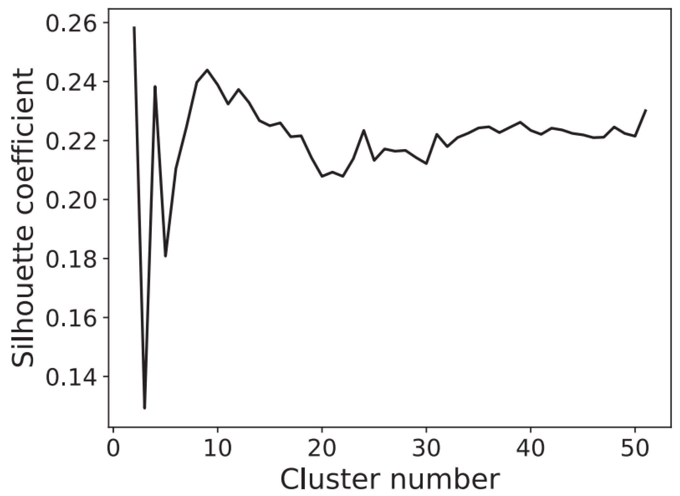
2.3. Clustering Methods to Distinguish Aerosol Types
2.3.1. The 2-D Clustering Method
2.3.2. Multi-Dimensional Mahalanobis Distance Clustering Method
3. Results
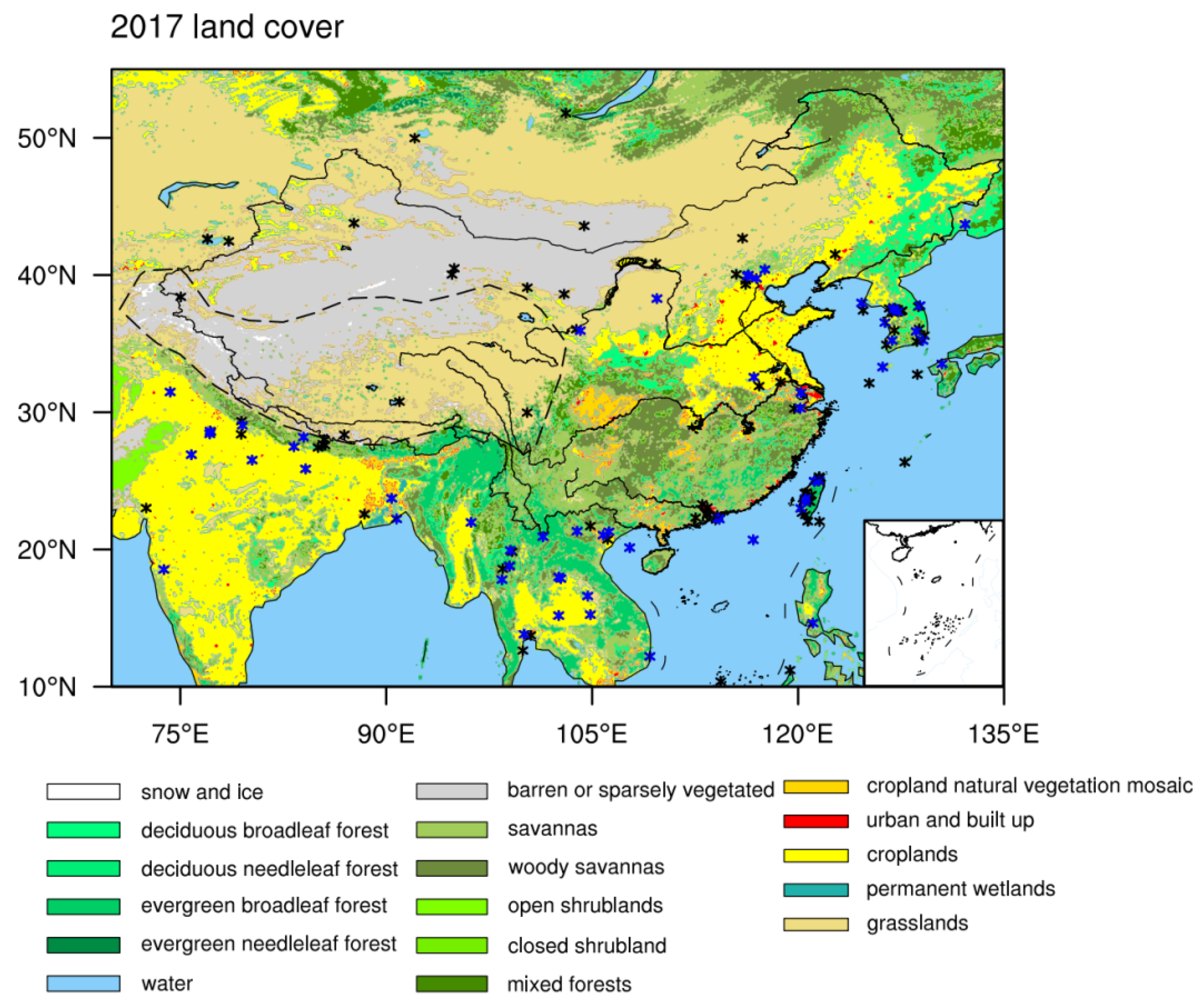
3.1. Land Cover and Meteorological States
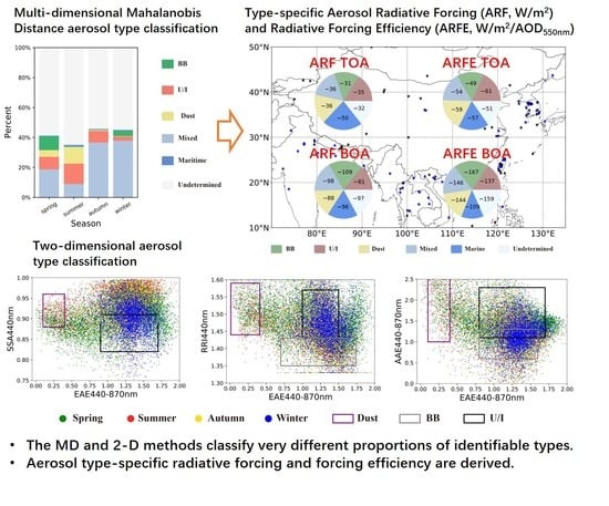
3.2. Aerosol Classification Using Multi-Dimensional Mahalanobis Distance Method
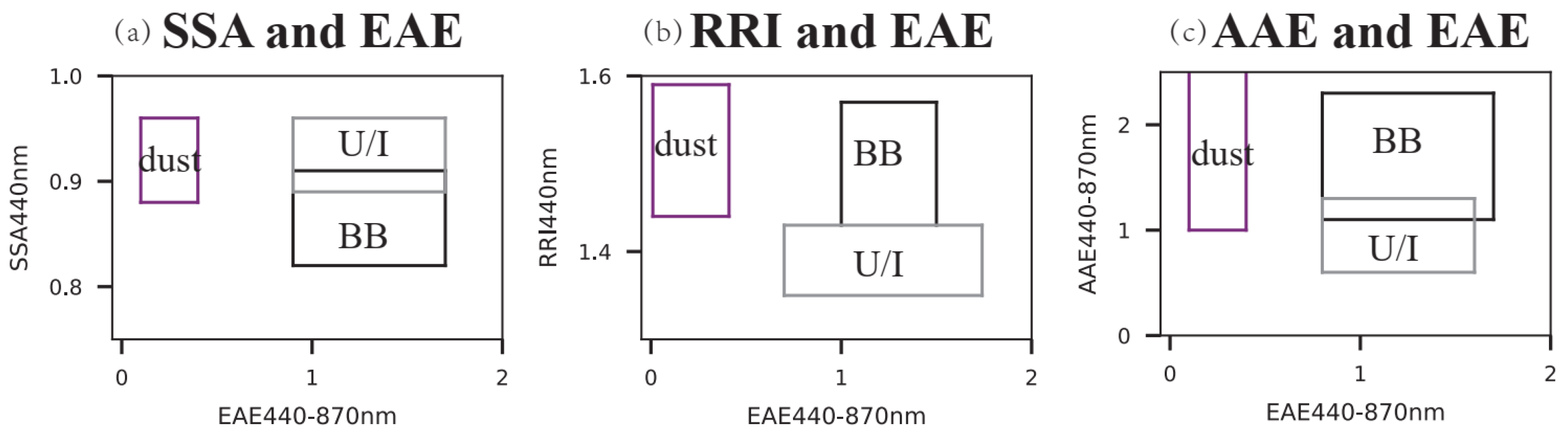
3.3. Aerosol Characteristics Identified by the 2-D Methods
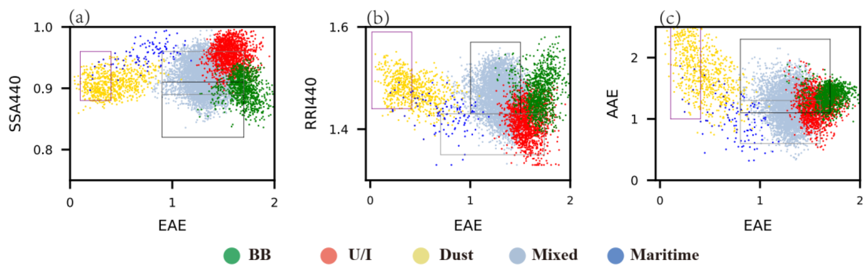
3.3.1. The 2-D Aerosol Classification Using AAE and EAE
3.3.2. The 2-D Aerosol Classification Using SSA and EAE
3.3.3. The 2-D Aerosol Classification Using RRI and EAE
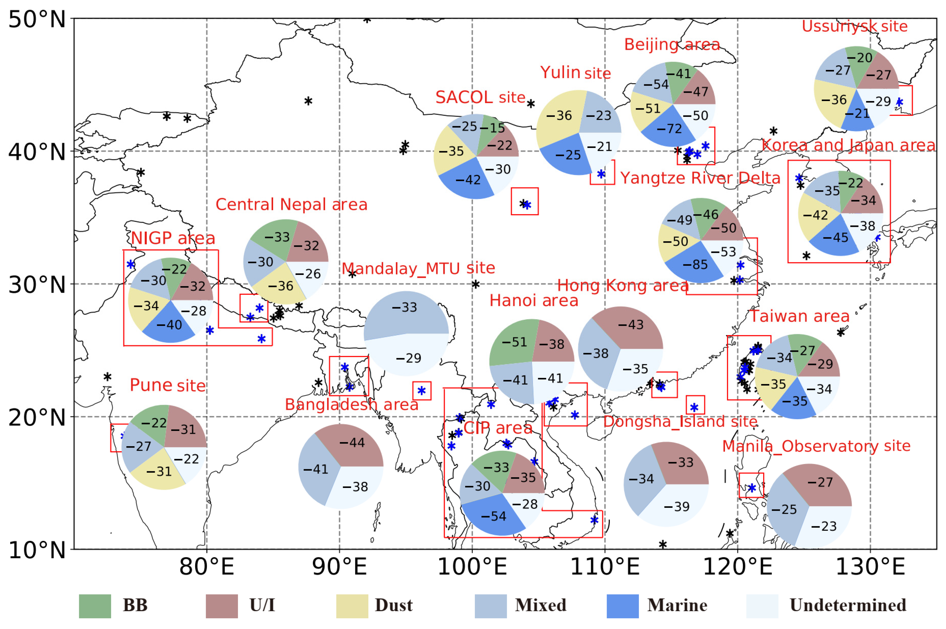
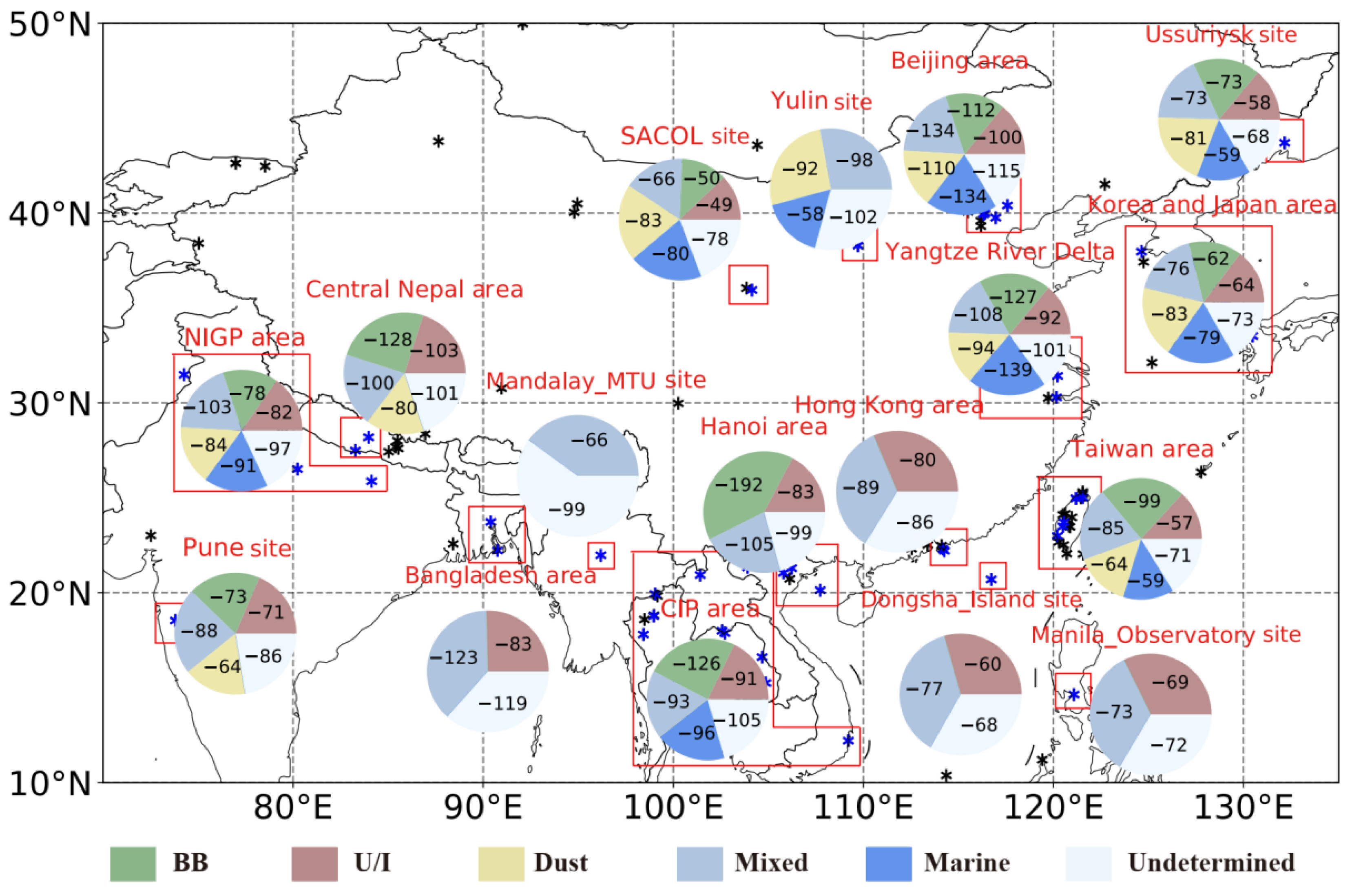
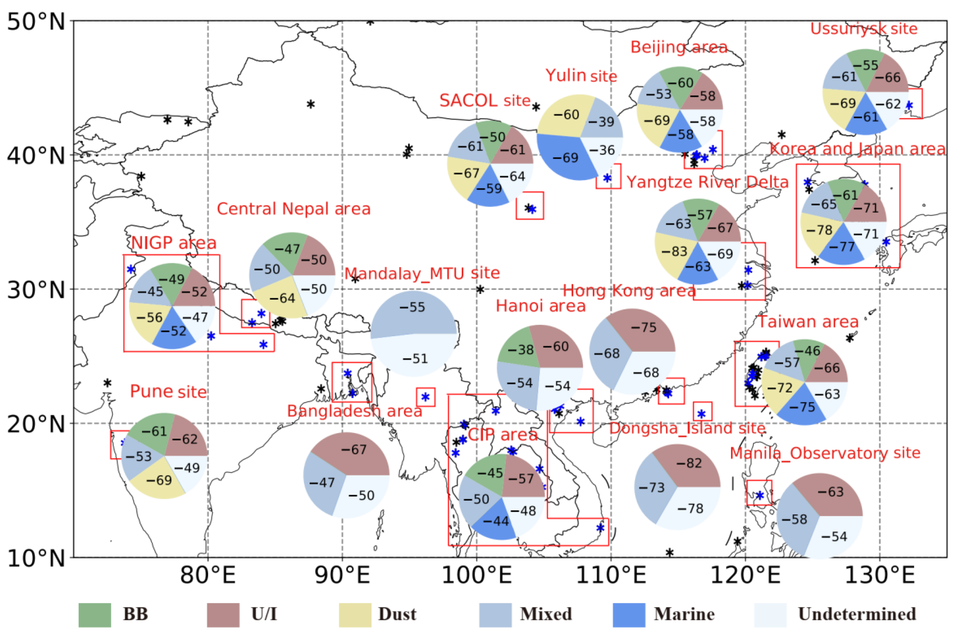
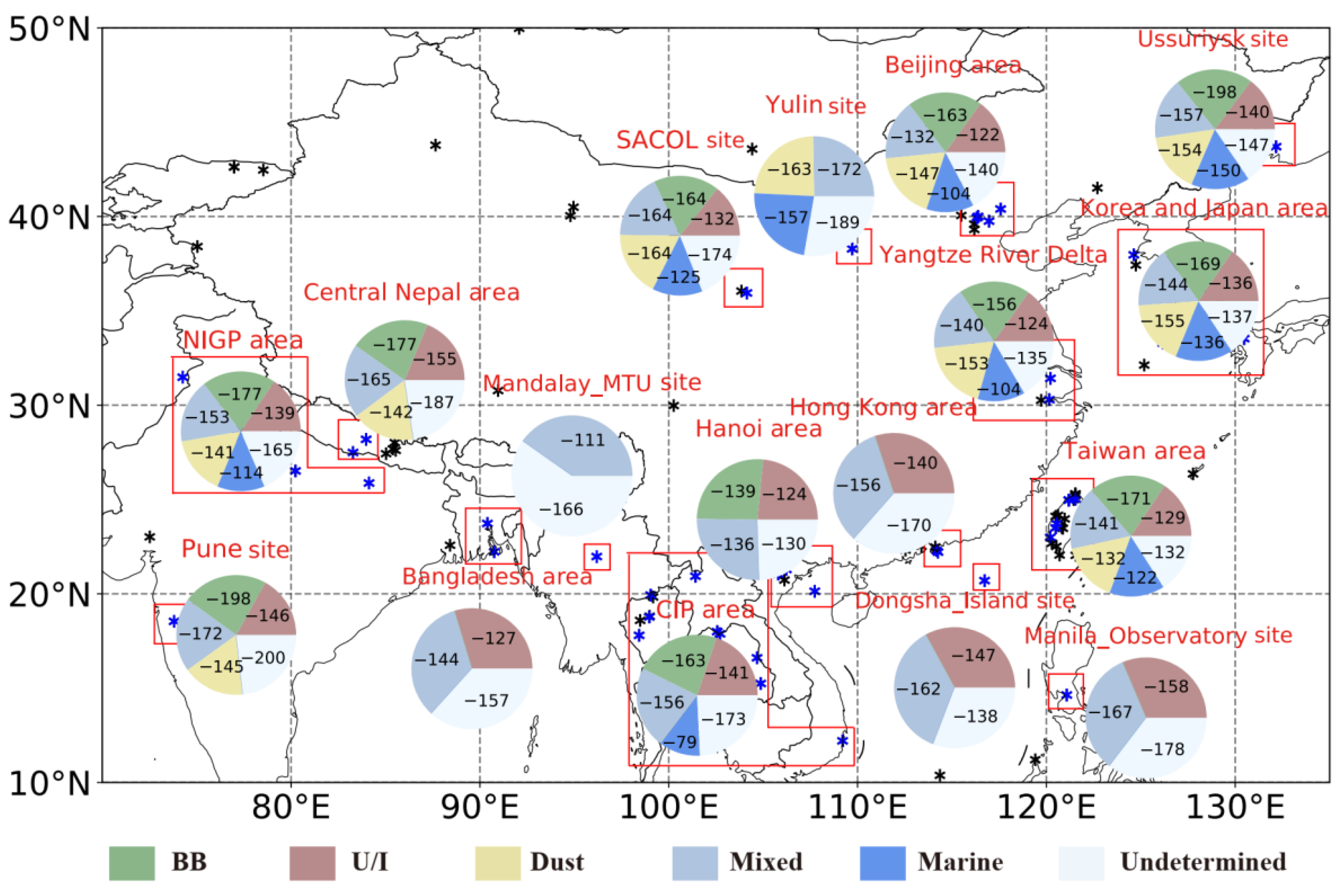
3.4. Aerosol Radiative Forcing and Radiative Forcing Efficiencies of Various Aerosol Types
4. Discussion
4.1. The Differences in the Proportions of Various Aerosol Type Classified by 2-D and MD Methods
4.2. The Differences in Aerosol Radiative Forcing and Forcing Efficiency by the 2-D and MD Classification
5. Conclusions
Supplementary Materials
Author Contributions
Funding
Data Availability Statement
Acknowledgments
Conflicts of Interest
Appendix A
References
- Boucher, O.; Randall, D.; Artaxo, P.; Bretherton, C.; Feingold, G.; Forster, P.; Kerminen, V.M.; Kondo, Y.; Liao, H.; Lohmann, U.; et al. Clouds and aerosols. In Climate Change 2013: The Physical Science Basis. Contribution of Working Group I to the Fifth Assessment Report of the Intergovernmental Panel on Climate Change; Stocker, T.F., Qin, D., Plattner, G.K., Tignor, M., Allen, S.K., Boschung, J., Nauels, A., Xia, Y., Bex, V., Midgley, P.M., Eds.; Cambridge University Press: Cambridge, UK; New York, NY, USA, 2013. [Google Scholar]
- Sakerin, S.M.; Pavlov, A.N.; Bukin, O.A.; Kabanov, D.M.; Kornienko, G.I.; Pol’kin, V.V.; Stolyarchuk, S.Y.; Turchinovich, Y.S.; Shmirko, K.A.; Mayor, A.Y. Results of an integrated aerosol experiment in the continent-ocean transition zone (Primorye and the Sea of Japan); Part 1: Variations of atmospheric aerosol optical depth and vertical profiles. Atmos. Ocean. Opt. 2011, 24, 64–73. [Google Scholar] [CrossRef]
- Hsu, C.Y.; Chiang, H.C.; Lin, S.L.; Chen, M.J.; Lin, T.Y.; Chen, Y.C. Elemental characterization and source apportionment of PM10 and PM2.5 in the western coastal area of central Taiwan. Sci. Total Environ. 2015, 541, 1139–1150. [Google Scholar] [CrossRef]
- Duc, H.N.; Bang, H.Q.; Quan, N.H.; Quang, N.X. Impact of biomass burnings in Southeast Asia on air quality and pollutant transport during the end of the 2019 dry season. Environ. Monit. Assess. 2021, 193, 565. [Google Scholar] [CrossRef] [PubMed]
- Lei, Y.L.; Shen, Z.X.; Wang, Q.Y.; Zhang, T.; Cao, J.J.; Sun, J.; Zhang, Q.; Wang, L.Q.; Xu, H.M.; Tian, J.; et al. Optical characteristics and source apportionment of brown carbon in winter PM2.5 over Yulin in Northern China. Atmos. Res. 2018, 213, 27–33. [Google Scholar] [CrossRef]
- Twomey, S. Influence of Pollution on the Shortwave Albedo of Clouds. J. Atmos. Sci. 1977, 34, 1149–1152. [Google Scholar] [CrossRef] [Green Version]
- Li, Z.Q.; Lau, W.K.M.; Ramanathan, V.; Wu, G.; Ding, Y.; Manoj, M.G.; Liu, J.; Qian, Y.; Li, J.; Zhou, T.; et al. Aerosol and monsoon climate interactions over Asia. Rev. Geophys. 2016, 54, 866–929. [Google Scholar] [CrossRef]
- Hua, Y.; Wang, S.X.; Jiang, J.K.; Zhou, W.; Xu, Q.C.; Li, X.X.; Liu, B.X.; Zhang, D.W.; Zheng, M. Characteristics and sources of aerosol pollution at a polluted rural site southwest in Beijing, China. Sci. Total Environ. 2018, 626, 519–527. [Google Scholar] [CrossRef]
- Mishra, A.K.; Shibata, T. Synergistic analyses of optical and microphysical properties of agricultural crop residue burning aerosols over the Indo-Gangetic Basin (IGB). Atmos. Environ. 2012, 57, 205–218. [Google Scholar] [CrossRef]
- Kim, Y.J. Asian Dust particles impacts on air quality and radiative forcing over Korea. In IOP Conference Series: Earth and Environmental Science; IOP Publishing: Bristol, UK, 2009; Volume 7, p. 012005. [Google Scholar] [CrossRef]
- Guo, J.; Deng, M.J.; Lee, S.S.; Wang, F.; Li, Z.Q.; Zhai, P.M.; Liu, H.; Lv, W.T.; Yao, W.; Li, X.W. Delaying precipitation and lightning by air pollution over the Pearl River Delta. Part I: Observational analyses. J. Geophys. Res. Atmos. 2016, 121, 6472–6488. [Google Scholar] [CrossRef]
- Liu, Y.U.; Sun, J.R.; Yang, B. The effects of black carbon and sulphate aerosols in China regions on East Asia monsoons. Tellus 2009, 61, 642–656. [Google Scholar] [CrossRef] [Green Version]
- Jiang, J.H.; Su, H.; Huang, L.; Wang, Y.; Massie, S.; Zhao, B.; Omar, A.; Wang, Z.E. Contrasting effects on deep convective clouds by different types of aerosols. Nat. Commun. 2018, 9, 3874. [Google Scholar] [CrossRef]
- Holben, B.N.; Eck, T.F.; Slutsker, I.; Smirnov, A.; Sinyuk, A.; Schafer, V.; Giles, D.; Dubovik, O. Aeronet’s Version 2.0 quality assurance criteria. Remote Sens. Atmos. Clouds 2006, 6408, 64080Q. [Google Scholar] [CrossRef]
- Che, H.Z.; Zhang, X.Y.; Chen, H.B.; Damiri, B.; Goloub, P.; Li, Z.Q.; Zhang, X.C.; Wei, Y.; Zhou, H.G.; Dong, F.; et al. Instrument calibration and aerosol optical depth validation of the China aerosol remote sensing network. J. Geophys. Res. Atmos. 2009, 114, D03206. [Google Scholar] [CrossRef]
- Li, Z.Q.; Xu, H.; Li, K.T.; Li, D.H.; Xie, Y.S.; Li, L.; Zhang, Y.; Gu, X.F.; ZHao, W.; Tian, Q.J.; et al. Comprehensive study of optical, physical, chemical, and radiative properties of total columnar atmospheric aerosols over China: An overview of sun–Sky radiometer observation network measurements. Bull. Amer. Meteor. Soc. 2018, 99, 739–755. [Google Scholar] [CrossRef]
- Hamill, P.; Giordano, M.; Ward, C.; Giles, D.; Holbene, B. An AERONET-Based aerosol classification using the Mahalanobis distance. Atmos. Environ. 2016, 140, 213–233. [Google Scholar] [CrossRef]
- Li, Z.; Zhang, Y.; Xu, H.; Li, K.; Dubovik, O.; Goloub, P. The Fundamental Aerosol Models over China Region: A Cluster Analysis of the Ground-Based Remote Sensing Measurements of Total Columnar Atmosphere. Geophys. Res. Lett. 2019, 46, 4924–4932. [Google Scholar] [CrossRef]
- Zheng, Y.; Che, H.Z.; Xia, X.G.; Wang, Y.Q.; Yang, L.K.; Chen, J.; Wang, H.; Zhao, H.J.; Li, L.; Zhang, L.; et al. Aerosol optical properties and its type classification based on multiyear joint observation campaign in north China plain megalopolis. Chemosphere 2020, 273, 128560. [Google Scholar] [CrossRef] [PubMed]
- Chen, H.; Cheng, T.H.; Gu, X.F.; Wu, Y. Characterization of aerosols in Beijing during severe aerosol loadings. Atmos. Environ. 2015, 119, 273–281. [Google Scholar] [CrossRef]
- Bibi, H.; Alam, K.; Bibi, S. In-depth discrimination of aerosol types using multiple clustering techniques over four locations in Indo-Gangetic plains. Atmos. Res. 2016, 181, 106–114. [Google Scholar] [CrossRef]
- Russell, P.B.; Bergstrom, R.W.; Shinozuka, Y.; Clarke, A.D.; DeCarlo, P.F.; Jimenez, J.L.; Livingston, J.M.; Redemann, J.; Dubovik, O.; Strawa, A. Absorption Angstrom Exponent in AERONET and related data as an indicator of aerosol composition. Atmos. Chem. Phys. 2010, 10, 1155–1169. [Google Scholar] [CrossRef] [Green Version]
- Xia, X.G.; Li, Z.Q.; Holben, B.; Wang, P.C.; Eck, T.; Chen, H.B.; Cribb, M.; Zhao, Y.X. Aerosol optical properties and radiative effects in the Yangtze Delta region of China. J. Geophys. Res. 2007, 112, D22S12. [Google Scholar] [CrossRef]
- Lau, K.M.; Kim, M.K.; Kim, K.M. Asian summer monsoon anomalies induced by aerosol direct forcing: The role of the Tibetan Plateau. Clim. Dyn. 2006, 26, 855–864. [Google Scholar] [CrossRef] [Green Version]
- Liu, J.J.; Zheng, Y.F.; Li, Z.Q.; Flynn, C.; Cribb, M. Seasonal variations of aerosol optical properties, vertical distribution and associated radiative effects in the Yangtze Delta region of China. J. Geophys. Res. Atmos. 2012, 117, D00K38. [Google Scholar] [CrossRef]
- Gautam, R.; Hsu, N.C.; Tsay, S.C.; Lau, K.M.; Holben, B.; Bell, S.; Smirnov, A.; Li, C.; Hansell, R.; Ji, Q.; et al. Accumulation of aerosols over the Indo-Gangetic plains and southern slopes of the Himalayas: Distribution, properties and radiative effects during the 2009 pre-monsoon season. Atmos. Chem. Phys. 2011, 11, 12841–12863. [Google Scholar] [CrossRef] [Green Version]
- Pavlidis, V.; Katragkou, E.; Prein, A.; Georgoulias, A.K.; Kartsios, S.; Zanis, P.; Karacostas, T. Investigating the sensitivity to resolving aerosol interactions in downscaling regional model experiments with WRFv3.8.1 over Europe. Geosci. Model Dev. 2020, 13, 2511–2532. [Google Scholar] [CrossRef]
- Wang, H.; Zhang, X.Y.; Gong, S.L.; Chen, Y.; Shi, G.Y.; Li, W. Radiative feedback of dust aerosols on the East Asian dust storms. J. Geophys. Res. 2010, 115, D23214. [Google Scholar] [CrossRef]
- Déandreis, C.; Balkanski, Y.; Dufresne, J.L.; Cozic, A. Radiative forcing estimates of sulfate aerosol in coupled climate-chemistry models with emphasis on the role of the temporal variability. Atmos. Chem. Phys. 2012, 12, 5583–5602. [Google Scholar] [CrossRef] [Green Version]
- Li, L.; Li, Z.; Li, K.; Wang, Y.; Tian, Q.; Su, X.; Yang, L.; Ye, S.; Xu, H. Aerosol Direct Radiative Effects over China Based on Long-Term Observations within the Sun–Sky Radiometer Observation Network (SONET). Remote Sens. 2020, 12, 3296. [Google Scholar] [CrossRef]
- Markowicz, K.M.; Zawadzka-Manko, O.; Lisok, J.; Chilinski, M.T.; Xian, P. The impact of moderately absorbing aerosol on surface sensible, latent, and net radiative fluxes during the summer of 2015 in Central Europe. J. Aerosol. Sci. 2020, 151, 105627. [Google Scholar] [CrossRef]
- García, O.E.; Díaz, J.P.; Expósito, F.J.; Díaz, A.M.; Dubovik, O.; Derimian, Y.; Dubuisson, P.; Roger, J.C. Shortwave radiative forcing and efficiency of key aerosol types using AERONET data. Atmos. Chem. Phys. 2012, 12, 5129–5145. [Google Scholar] [CrossRef] [Green Version]
- Dubovik, O.; Holben, B.; Eck, T.F.; Smirnov, A.; Kaufman, Y.J.; King, M.D.; Tanré, D.; Slutsker, I. Variability of absorption and optical properties of key aerosol types observed in worldwide locations. J. Atmos. Sci. 2002, 59, 590–608. [Google Scholar] [CrossRef]
- Latha, R.; Murthy, B.S.; Kumar, M.; Lipi, K.; Jyotsna, S. Aerosol radiative forcing controls: Results from an Indian table-top mining region. Atmos. Environ. 2013, 81, 687–694. [Google Scholar] [CrossRef]
- Sulla-Menashe, D.; Gray, J.M.; Abercrombie, S.P.; Friedla, M.A. Hierarchical mapping of annual global land cover 2001 to present: The MODIS Collection 6 Land Cover product. Remote. Sens. Environ. 2019, 222, 183–194. [Google Scholar] [CrossRef]
- Dee, D.P.; Uppala, S.M.; Simmons, A.J.; Berrisford, P.; Poli, P.; Kobayashi, S.; Andrae, U.; Balmaseda, M.A.; Balsamo, G.; Bauer, P.; et al. The ERA-Interim reanalysis: Configuration and performance of the data assimilation system. Q. J. R. Meteorol. Soc. 2011, 137, 553–597. [Google Scholar] [CrossRef]
- Huffman, G.J.; Bolvin, D.T.; Nelkin, E.J.; Adler, R.F. TRMM (TMPA) Precipitation L3 1 Day 0.25 Degree X 0.25 Degree V7; Andrey, S., Ed.; Goddard Earth Sciences Data and Information Services Center (GES DISC), 2016. Available online: https://disc.gsfc.nasa.gov/datasets/TRMM_3B42_Daily_7/summary (accessed on 15 March 2022). [CrossRef]
- Fox, W.R. Review of Finding Groups in Data: An Introduction to Cluster Analysis; Kaufman, L., Rousseeuw, P.J., Eds.; Journal of the Royal Statistical Society. Series C; Wiley: Hoboken, NJ, USA, 1991; Volume 40, pp. 486–487. [Google Scholar] [CrossRef]
- Rousseeuw, P.J. Silhouettes: A graphical aid to the interpretation and validation of cluster analysis. J. Comput. Appl. Math. 1987, 20, 53–65. [Google Scholar] [CrossRef] [Green Version]
- Mahalanobis, P.C. On the generalized distance in statistics. Proc. Natl. Inst. Sci. India 1936, 2, 49–55. [Google Scholar]
- Huang, K.; Fu, J.S.; Hsu, N.C.; Gao, Y.; Dong, X.Y.; Tsay, S.C.; Lam, Y.F. Impact assessment of biomass burning on air quality in Southeast and East Asia during BASE-ASIA. Atmos. Environ. 2013, 78, 291–302. [Google Scholar] [CrossRef] [Green Version]
- Ding, Y.H.; Chan, J. The East Asian summer monsoon: An overview. Meteorol. Atmos. Phys. 2005, 89, 117–142. [Google Scholar] [CrossRef]
- Prijith, S.S.; Babu, S.S.; Lakshmi, N.B.; Satheesh, S.K.; Moorthy, K.K. Meridional gradients in aerosol vertical distribution over Indian Mainland: Observations and model simulations. Atmos. Environ. 2016, 125, 337–345. [Google Scholar] [CrossRef]
- Kansakar, S.R.; Hannah, D.M.; Gerrard, J.; Rees, R. Spatial pattern in the precipitation regime of Nepal. Int. J. Climatol. 2004, 24, 1645–1659. [Google Scholar] [CrossRef]
- Li, J.; Zhang, Y.Q.; Wang, Z.F.; Sun, Y.L.; Fu, P.Q.; Yang, Y.C.; Huang, H.L.; Li, J.J.; Zhang, Q.; Lin, C.Y.; et al. Regional impact of biomass burning in Southeast Asia on atmospheric aerosols during the 2013 Seven South-East Asian Studies Project. Aerosol Air Qual. Res. 2017, 17, 2924–2941. [Google Scholar] [CrossRef]
- Kozlov, V.S.; Pol’kin, V.V.; Panchenko, M.V.; Golobokova, L.P.; Turchinovich, U.S.; Hodzher, T.V. Results of integrated aerosol experiment in the continent-ocean transition zone (Primorye and the Japan Sea). Part 3. Microphysical characteristics and ion composition of aerosol in the near-ground and near-water layers. Atmos. Ocean. Opt. 2011, 24, 207–217. [Google Scholar] [CrossRef]
- Ozdemir, E.; Tuygun, G.T.; Elbir, T. Application of aerosol classification methods based on AERONET version 3 product over eastern Mediterranean and Black Sea. Atmos. Pollut. Res. 2020, 11, 2226–2243. [Google Scholar] [CrossRef]
- Zhang, L.; Zheng, X.S. Spatial-temporal Variation of Aerosol Optical Properties in Coastal Region, China Based on CALIPSO Data. J. Earth Sci. Environ. 2021, 43, 1033–1049. [Google Scholar] [CrossRef]
- Dementeva, A.; Zhamsueva, G.; Zayakhanov, A.; Tcydypov, V. Interannual and Seasonal Variation of Optical and Microphysical Properties of Aerosol in the Baikal Region. Atmosphere 2022, 13, 211. [Google Scholar] [CrossRef]
- Stefan, S.; Voinea, S.; Iorga, G. Study of the aerosol optical characteristics over the Romanian Black Sea Coast using AERONET data. Atmos. Pollut. Res. 2020, 11, 1165–1178. [Google Scholar] [CrossRef]
- Cuneo, L.; Ulke, A.G.; Cerne, B. Advances in the characterization of aerosol optical properties using long-term data from AERONET in Buenos Aires. Atmos. Pollut. Res. 2022, 13, 101360. [Google Scholar] [CrossRef]
- Rupakheti, D.; Adhikary, B.; Praveen, P.S.; Rupakheti, M.; Kang, S.C.; Mahata, K.S.; Naja, M.; Zhang, Q.G.; Panday, A.K.; Lawrence, M.G. Pre-monsoon air quality over Lumbini, a world heritage site along the Himalayan foothills. Atmos. Chem. Phys. 2017, 17, 11041–11063. [Google Scholar] [CrossRef] [Green Version]
- Rupakheti, D.; Kang, S.C.; Rupakheti, M.; Cong, Z.Y.; Tripathee, L.; Panday, A.K.; Holben, B.N. Observation of optical properties and sources of aerosols at Buddha’s birthplace, Lumbini, Nepal: Environmental implications. Environ. Sci. Pollut. Res. 2018, 25, 14868–14881. [Google Scholar] [CrossRef] [PubMed]
- Cao, C.X.; Zheng, S.; Singh, R.P. Characteristics of aerosol optical properties and meteorological parameters during three major dust events (2005–2010) over Beijing, China. Atmos. Res. 2014, 150, 129–142. [Google Scholar] [CrossRef]
- Du, C.L.; Li, X.M.; Chen, C.; Wang, F.Q.; Peng, Y.; Dong, Y.; Dong, Z.P. Concentration variation and absorption charracteristics of black carbon during autumn and winter in Yulin near Mu Us Sandy Land. J. Desert Res. 2014, 34, 869–877. [Google Scholar] [CrossRef]
- Yan, C.Q.; Zheng, M.; Sullivan, A.P.; Bosch, C.; Desyaterik, Y.; Andersson, A.; Li, X.Y.; Guo, X.S.; Zhou, T.; Gustafssonc, Ö.; et al. Chemical characteristics and light-absorbing property of water-soluble organic carbon in Beijing: Biomass burning contributions. Atmos. Environ. 2015, 121, 4–12. [Google Scholar] [CrossRef] [Green Version]
- You, C.; Gao, S.P.; Xu, C. Biomass burning emissions contaminate winter snowfalls in urban Beijing: A case study in 2012. Atmos. Pollut. Res. 2015, 6, 376–381. [Google Scholar] [CrossRef] [Green Version]
- Yang, Y.; Li, X.R.; Shen, R.R.; Liu, Z.R.; Ji, D.S.; Wang, Y.S. Seasonal variation and sources of derivatized phenols in atmospheric fine particulate matter in North China Plain. J. Atmos. Sci. 2020, 89, 139–147. [Google Scholar] [CrossRef]
- Cheng, Y.; Engling, G.; He, K.B.; Duan, F.K.; Ma, Y.L.; Du, Z.Y.; Liu, J.M.; Zheng, M.; Weber, R.J. Biomass burning contribution to Beijing aerosol. Atmos. Chem. Phys. 2013, 13, 7765–7781. [Google Scholar] [CrossRef] [Green Version]
- Emilenko, A.S.; Isakov, A.A.; Kopeikin, V.M.; Wang, G.C. Relative contributions of regional, urban, and local sources of atmospheric aerosol pollution in regions with different levels of anthropogenic load. In 21st International Symposium Atmospheric and Ocean Optics: Atmospheric Physics; SPIE: Bellingham, WA, USA, 2015; Volume 9680, p. 968046. [Google Scholar] [CrossRef]
- Dong, X.; Fu, J.S. Understanding interannual variations of biomass burning from Peninsular Southeast Asia, part II: Variability and different influences in lower and higher atmosphere levels. Atmos. Environ. 2015, 115, 9–18. [Google Scholar] [CrossRef]
- Sang, X.F.; Chan, C.Y.; Engling, G.; Chan, L.Y.; Wang, X.M.; Zhang, Y.N.; Shi, S.; Zhang, Z.S.; Zhang, T.; Hu, M. Levoglucosan enhancement in ambient aerosol during springtime transport events of biomass burning smoke to southeast China. Tellus B Chem. Phys. Meteorol. 2011, 63, 129–139. [Google Scholar] [CrossRef]
- Ding, A.; Wang, T.; Fu, C. Transport characteristics and origins of carbon monoxide and ozone in Hong Kong, south China. J. Geophys. Res. Atmos. 2013, 118, 9475–9488. [Google Scholar] [CrossRef]
- Logan, T.; Xi, B.K.; Dong, X.Q. A Comparison of the Mineral Dust Absorptive Properties between Two Asian Dust Events. Atmosphere 2015, 4, 1–16. [Google Scholar] [CrossRef] [Green Version]
- Choi, J.K.; Heo, J.B.; Ban, S.J.; Yi, S.M.; Zoh, K.D. Source apportionment of PM2.5 at the coastal area in Korea. Sci. Total Environ. 2013, 447, 370–380. [Google Scholar] [CrossRef]
- Shon, Z.H. Long-term variations in PM2.5 emission from open biomass burning in Northeast Asia derived from satellite-derived data for 2000–2013. Atmos. Environ. 2015, 107, 342–350. [Google Scholar] [CrossRef]
- Titos, G.; Burgos, M.A.; Zieger, P.; Alados-Arboledas, L.; Baltensperger, U.; Jefferson, A.; Sherman, J.; Weingartner, E.; Henzing, B.; Luoma, K.; et al. A global study of hygroscopicity-driven light-scattering enhancement in the context of other in situ aerosol optical properties. Atmos. Chem. Phys. 2021, 21, 13031–13050. [Google Scholar] [CrossRef]
- Yoon, S.C.; Kim, J. Influences of relative humidity on aerosol optical properties and aerosol radiative forcing during ACE-Asia. Atmos. Environ. 2006, 40, 4328–4338. [Google Scholar] [CrossRef]


| Aerosol Types | Thresholds | |||||
|---|---|---|---|---|---|---|
| SSA and EAE | RRI and EAE | AAE and EAE | ||||
| SSA | EAE | RRI | EAE | AAE | EAE | |
| U/I | 0.89–0.96 | 0.90–1.70 | 1.35–1.43 | 0.70–1.74 | 0.60–1.30 | 0.80–1.60 |
| Dust | 0.88–0.96 | 0.10–0.40 | 1.44–1.59 | 0.01–0.41 | 1.00–3.00 | 0.01–0.40 |
| BB | 0.82–0.91 | 0.90–1.70 | 1.43–1.57 | 1.00–1.50 | 1.10–2.30 | 0.80–1.70 |
| Aerosol Type | SSA | EAE | RRI | AAE | IRI |
|---|---|---|---|---|---|
| BB | 0.89 | 1.87 | 1.48 | 1.3 | 0.02 |
| U/I | 0.96 | 1.76 | 1.4 | 1.15 | 0.005 |
| Dust | 0.91 | 0.28 | 1.47 | 1.75 | 0.004 |
| Mixed | 0.92 | 1.32 | 1.45 | 1.2 | 0.011 |
| Marine | 0.97 | 0.59 | 1.4 | 0.93 | 0.001 |
| MS 1 | MS 2 | MS 3 | MS 4 | MS 5 | MS 6 | MS 7 | MS 8 | MS 9 | |
|---|---|---|---|---|---|---|---|---|---|
| T (°C) | 25.6 | 28.2 | 26.7 | 17.3 | 12.7 | 21.3 | 20.5 | 21.2 | 25.8 |
| PR (mm/d) | 5.6 | 2.7 | 4 | 4.2 | 1 | 4.2 | 0.2 | 1.2 | 5.2 |
| U (m/s) | −3 | 0.6 | 3 | −0.2 | 0.9 | −2.9 | −1.1 | 1.2 | 0.4 |
| V (m/s) | −1 | −0.1 | −2.2 | −1.1 | −0.3 | −3.3 | −1.2 | 0.5 | 0.5 |
| RH (%) | 78.9 | 59.3 | 75.1 | 73.7 | 55.6 | 81.2 | 31.1 | 60.3 | 78.1 |
| TCC (%) | 60.8 | 31.4 | 45 | 55.4 | 42.7 | 49.7 | 36.2 | 53.5 | 58.9 |
| σ2 (T) | 1.7 | 2.2 | 0 | 13.2 | 22.5 | 1.9 | 3 | 4.2 | 4.8 |
| σ2 (PR) | 2.2 | 1.6 | 2 | 1.4 | 0.5 | 0.4 | 0 | 0.4 | 4.4 |
| σ2 (U) | 1.4 | 0.4 | 0 | 1.1 | 0.8 | 0.3 | 1.1 | 1 | 0.7 |
| σ2 (V) | 0.3 | 0.2 | 0.1 | 0.5 | 0.4 | 0.3 | 0.3 | 0.4 | 0.4 |
| σ2 (RH) | 1.8 | 59.3 | 3 | 11.4 | 128.7 | 1.7 | 23.7 | 99.8 | 17.4 |
| σ2 (TCC) | 69.3 | 81.7 | 88.2 | 10.9 | 43.7 | 21.8 | 8.1 | 38.4 | 73.8 |
| Sub-Region | AERONET Sites |
|---|---|
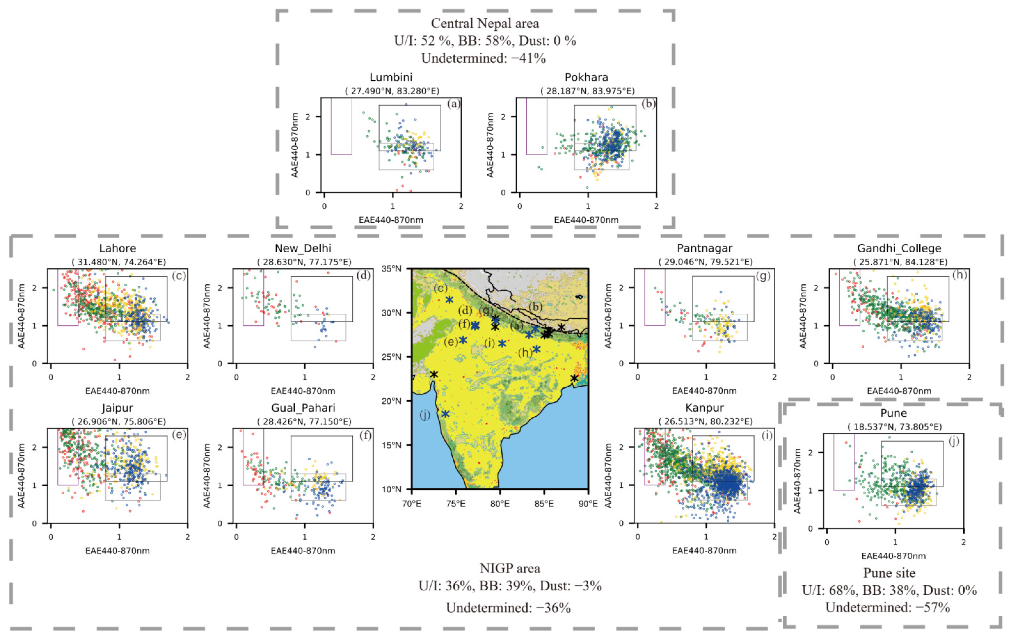
| NIGP area | New_Delhi, Gual_Pahari, Lahore, Pantnagar, Kanpur, Gandhi_College, Jaipur |
| Central Nepal area | Pokhara, Lumbini |
| Bangladesh area | Dhaka_University, Bhola |
| CIP area | Chiang_Mai_Met_Sta, Doi_Ang_Khang, Omkoi, Son_La, Luang_Namtha, Nong_Khai, Vientiane, Pimai, Mukdahan, Silpakorn_Univ, Ubon_Ratchathani, NhaTrang |
| Hanoi area | NGHIA_DO, Bac_Giang, Bach_Long_Vy |
| Hong Kong area | Hong_Kong_PolyU, Hong_Kong_Hok_Tsui |
| Taiwan area | Taipei_CWB, EPA-NCU, NCU_Taiwan, Chiayi, Douliu, Chen-Kung_Univ |
| Yangtze River Delta | Taihu, Hangzhou_City, Shouxian |
| Korea and Japan area | Baengnyeong, Seoul_SNU, Yonsei_University, Hankuk_UFS, Anmyon, Gwangju_GIST, Gosan_SNU, Gangneung_WNU, KORUS_Kyungpook_NU, Pusan_NU, Fukuoka |
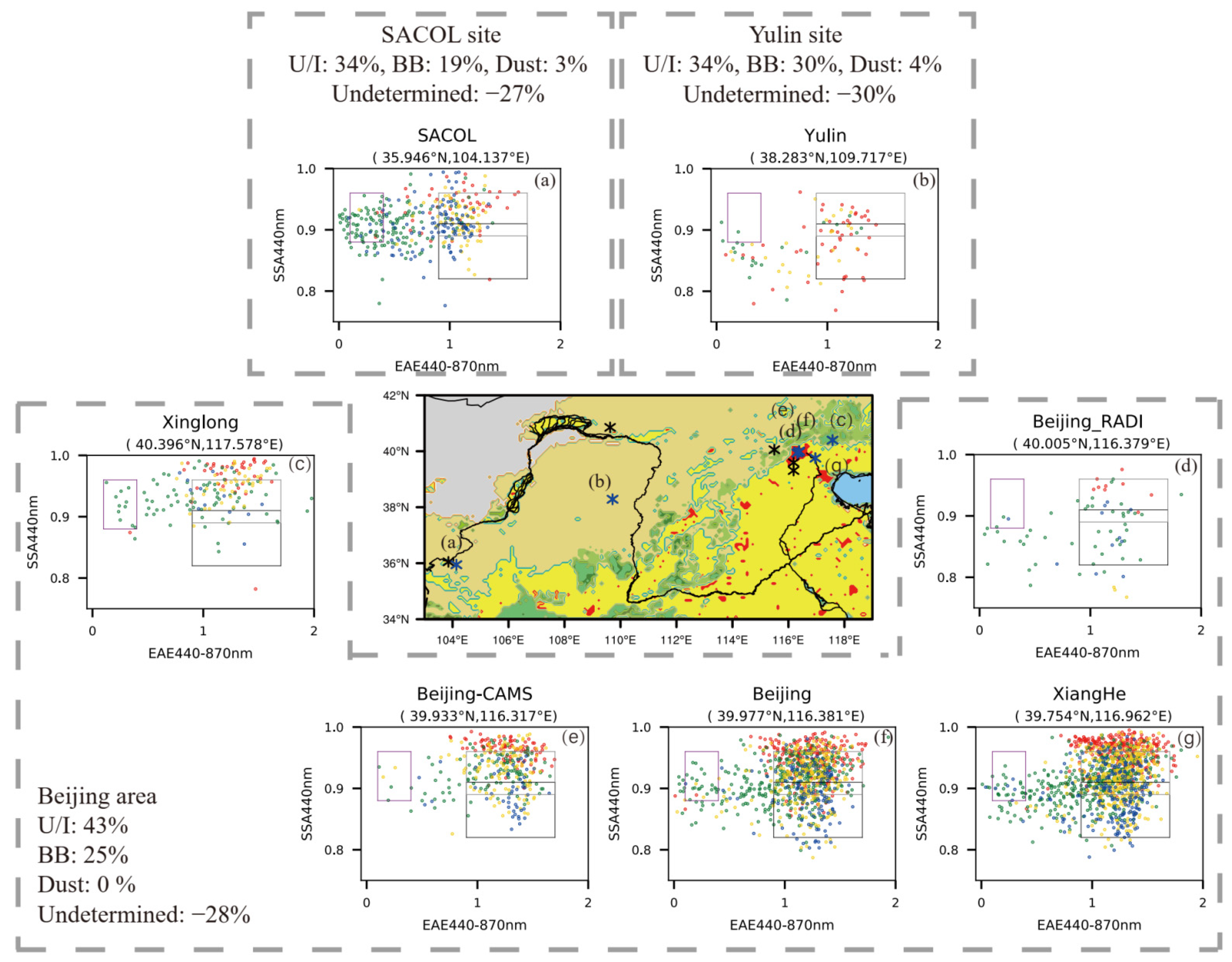
| Beijing area | Beijing_RADI, Beijing, Beijing-CAMS, XiangHe, Xinglong |
| Single sites | SACOL, Yulin, Ussuriysk, Pune, Dongsha_Island, Manila_Observatory, Mandalay_MTU |
| U/I | BB | Dust | |
|---|---|---|---|
| 2-D SSA-EAE | 49.7 | 32.5 | 43.7 |
| 2-D RRI-EAE | 56.3 | 6.3 | 48.1 |
| 2-D AAE-EAE | 39.8 | 50.1 | 47.7 |
| Aerosol Type | MD | 2-D Minus MD Difference | |||
|---|---|---|---|---|---|
| SSA-EAE | RRI-EAE | AAE-EAE | |||
| ARFBOA | BB | −104.4 | 6.3 | 7.4 | 10.0 |
| U/I | −85.7 | −7.9 | 1.7 | −6.4 | |
| Dust | −88.2 | −0.5 | −4.1 | −6.2 | |
| ARFTOA | BB | −31.3 | 4.9 | −3.4 | −4.9 |
| U/I | −35.3 | −2.4 | −1.5 | 4.0 | |
| Dust | −36.3 | −2.9 | −1.7 | −1.6 | |
| ARFEBOA | BB | −165.3 | −13.8 | 10.4 | 14.8 |
| U/I | −140.5 | −0.9 | 4.7 | −14.3 | |
| Dust | −146.1 | 5.0 | −0.5 | −0.5 | |
| ARFETOA | BB | −51.1 | 2.0 | −3.2 | −5.5 |
| U/I | −59.4 | 1.8 | 1.1 | 7.8 | |
| Dust | −60.3 | −2.4 | 0.2 | 2.0 | |
Publisher’s Note: MDPI stays neutral with regard to jurisdictional claims in published maps and institutional affiliations. |
© 2022 by the authors. Licensee MDPI, Basel, Switzerland. This article is an open access article distributed under the terms and conditions of the Creative Commons Attribution (CC BY) license (https://creativecommons.org/licenses/by/4.0/).
Share and Cite
Liu, Y.; Yi, B. Aerosols over East and South Asia: Type Identification, Optical Properties, and Implications for Radiative Forcing. Remote Sens. 2022, 14, 2058. https://doi.org/10.3390/rs14092058
Liu Y, Yi B. Aerosols over East and South Asia: Type Identification, Optical Properties, and Implications for Radiative Forcing. Remote Sensing. 2022; 14(9):2058. https://doi.org/10.3390/rs14092058
Chicago/Turabian StyleLiu, Yushan, and Bingqi Yi. 2022. "Aerosols over East and South Asia: Type Identification, Optical Properties, and Implications for Radiative Forcing" Remote Sensing 14, no. 9: 2058. https://doi.org/10.3390/rs14092058
APA StyleLiu, Y., & Yi, B. (2022). Aerosols over East and South Asia: Type Identification, Optical Properties, and Implications for Radiative Forcing. Remote Sensing, 14(9), 2058. https://doi.org/10.3390/rs14092058