Article

Classification of Tree Species in Different Seasons and Regions Based on Leaf Hyperspectral Images

1
School of Technology, Beijing Forestry University, Beijing 100083, China
2
Key Laboratory of State Forestry Administration on Forestry Equipment and Automation, Beijing 100083, China
*
Author to whom correspondence should be addressed.
Remote Sens. 2022, 14(6), 1524; https://doi.org/10.3390/rs14061524
Submission received: 19 January 2022 / Revised: 27 February 2022 / Accepted: 19 March 2022 / Published: 21 March 2022
(This article belongs to the Topic Artificial Intelligence in Sensors)

Abstract

:
This paper aims to establish a tree species identification model suitable for different seasons and regions based on leaf hyperspectral images, and to mine a more effective hyperspectral identification algorithm. Firstly, the reflectance spectra of leaves in different seasons and regions were analyzed. Then, to solve the problem that 0-element in sparse random (SR) coding matrices affects the classification performance of error-correcting output codes (ECOC), two versions of supervision-mechanism-based ECOC algorithms, namely SM-ECOC-V1 and SM-ECOC-V2, were proposed in this paper. In addition, the performance of the proposed algorithms was compared with that of six traditional algorithms based on all bands and feature bands. The experiment results show that seasonal and regional changes have an effect on the reflectance spectra of leaves, especially in the near-infrared region of 760–1000 nm. When the spectral information of different seasons and different regions is added into the identification model, tree species can be effectively classified. SM-ECOC-V2 achieves the best classification performance based on both all bands and feature bands. Furthermore, both SM-ECOC-V1 and SM-ECOC-V2 outperform the ECOC method under SR coding strategy, indicating the proposed methods can effectively avoid the influence of 0-element in SR coding matrix on classification performance.

Graphical Abstract

1. Introduction

Forest resources constitute the main body of the terrestrial ecosystem and are the basis of construction for forestry and ecological environment. They not only provide abundant material resources for human survival and development but also play an extremely important role in the sustainable development of economy, environment and society [1,2]. They can provide valuable information for estimating the economic value of forests and studying forest ecosystems to figure out the composition of forest tree species [3]. Therefore, the accurate identification of forest tree species is of great significance to the rational planning, utilization and protection of forest resources.
In recent years, using hyperspectral remote sensing technology to identify forest tree species has become a hot spot in forestry remote sensing research. Hyperspectral imaging technology is an organic combination of imaging technology and spectroscopy technology which can obtain tens to hundreds of spectral bands for each pixel and reflect the subtle differences between the reflectance spectra of different ground objects, thus greatly improving the identification ability of ground objects [4,5]. According to the different acquisition methods of hyperspectral data, it can be divided into satellite-borne hyperspectral data, airborne hyperspectral data and non-imaging hyperspectral data.
Satellite-borne hyperspectral remote sensing technology is convenient to realize the identification of forest tree species on a large scale. Many researchers have carried out research on forest tree species identification based on satellite-borne hyperspectral images obtained by EO-1/Hyperion, PROBA/CHRIS and HJ-1A/HSI hyperspectral sensors [6,7,8,9]. However, the satellite-borne hyperspectral sensor is far away from the ground, so it is limited by the spatial resolution. Therefore, this method can only identify the forest types or dominant tree species groups but cannot identify the specific species of individual trees, which makes it difficult to meet the research requirements of fine identification for forest tree species [2].
Airborne hyperspectral remote sensing technology is a detection technology that utilizes aircraft as the carrying tools of hyperspectral sensors to realize ground remote sensing operation. Unlike satellite-borne remote sensing technology that is restricted by satellite operation period and orbit, airborne remote sensing technology is convenient and flexible [10]. Lucas et al. classified mixed forests in Central South-East Queensland, Australia based on airborne CASI and HyMap hyperspectral data [11]. Richter et al. used airborne AISA DUAL hyperspectral data to classify 10 broadleaf tree species in a species-rich Central European forest area [12]. In addition, airborne LiDAR can accurately obtain the vertical structure information of forest stand, which is helpful to understand forest structure characteristics, extract canopy physical and chemical characteristics, and identify forest types [13]. In recent years, many researchers have fused airborne LiDAR data with hyperspectral images to carry out the research on identification of forest tree species [14,15,16]. This fusion technology can improve the identification accuracy of forest types with relatively complex forest structure to a certain extent, but it can only identify several main or dominant tree species in the forest. Thus, it is easily affected by weather and light conditions.
In terms of non-imaging hyperspectral data, researchers mainly utilized the hyperspectral data measured by non-imaging hyperspectral spectrometer in the field or laboratory to identify tree species from the perspective of leaves and canopy, and improved the identification accuracy of tree species by means of transformation of original spectral data such as normalization, logarithmic transformation, differential transformation and so on [17,18,19]. In addition, Clark et al. showed that the ability of leaf spectral features to identify vegetation was better than that of canopy spectral features [20]. The non-imaging spectrometer utilizes optical fiber probe to collect spectral information, in which the probe needs to be placed at a certain height so that the canopy or leaves of vegetation are within the view range of the probe. However, the view range of probe cannot be accurately controlled, resulting in a lot of background noises in the reflectance spectra, thus affecting the accuracy of tree species identification. Therefore, this paper utilized hyperspectral imaging technology to identify tree species at the leaf level.
Furthermore, some studies showed that seasonal and regional changes put an impact on the spectral response of tree leaves, thus affecting the identification of tree species [21,22,23]. However, researchers mostly established hyperspectral tree species identification models in a specific season and a specific geographical environment. Until now, there have been few reports on the establishment of hyperspectral tree species identification models suitable for different seasons and different regions.
To solve the above problems, this paper carries out research on tree species identification in different seasons and regions based on leaf hyperspectral images, aiming at establishing a hyperspectral tree species identification model suitable for different seasons and regions, and mining a more effective hyperspectral identification algorithm.

2. Materials and Methods

2.1. Experimental Materials

This study mainly relied on the vegetation in the campus of Beijing Forestry University. The leaves of 50 tree species were collected, in which 3 to 5 trees were selected for each tree species, 15 to 20 healthy leaves were randomly collected from each tree, and each leaf was taken as a sample. The serial number and specific name of each tree species are shown in Table 1.
To analyze the influence of different seasons on the spectral response of tree leaves, 20 tree species (No. 1–20) were selected from 50 tree species, and leaf samples of these 20 tree species were repeatedly collected in spring, summer and autumn. The specific collection time is shown in Figure 1a. The leaves of the other 30 species (No. 21–50) were all collected in summer.
To analyze the influence of different regions on the spectral response of tree leaves, the leaves of 5 tree species (No. 1–5) were collected on the campus of Beijing Forestry University and Xiling Lake Park of Wu’an City, Hebei Province (416 km from Beijing Forestry University), respectively. The specific collection time is shown in Figure 1b.
A total of 5717 leaf samples were collected in this study. In the process of sample collection, to ensure the freshness and biochemical indexes of the leaves, the collected leaves were classified and put into numbered, sealed bags, then placed in a fresh-keeping box with ice and then quickly brought back to the laboratory for acquisition of leaf hyperspectral images. During the process of acquisition of leaf hyperspectral images, the collected leaves were refrigerated in the refrigerator. In each experiment, the process from leaf collection to the end of leaf hyperspectral image acquisition was completed within 12 h, so as to ensure the freshness and biochemical indexes of leaves were as fair as possible.

2.2. Hyperspectral Image Acquisition

In this study, leaf hyperspectral images were acquired by a SOC710VP portable hyperspectral imaging spectrometer, which has a built-in translation push scanning device without additional scanning platform. Scanning speed and integration time can be automatically matched without manual adjustment, thus avoiding image distortion. The specific parameters of this equipment are shown in Table 2.
In the process of hyperspectral image acquisition, only the halogen lamp light source matched with the spectrometer was used, and each leaf was placed under the spectrometer lens with the front facing up. At the same time, the height of the spectrometer was adjusted to make the entire leaf within the field of vision of the spectrometer lens. To avoid the influence on the reflection spectra of leaves, black paper was placed under leaves as the background. Moreover, to eliminate the effect of the uneven distribution of light intensity at each band and the dark current in the camera on the spectral data, it is necessary to correct the original hyperspectral images. The acquisition and correction of hyperspectral images were completed in the software supporting the instrument, and the correction formula is as follows:
I = I 0 I D I W I D
where I represents the corrected hyperspectral image; I0 represent the original hyperspectral image; ID represents the dark reference image; and IW represents the white reference image.

2.3. Hyperspectral Data Extraction

In this study, the entire leaf was taken as the region of interest (ROI) to extract spectral data. Through screening, it is found that there is a clear boundary between the leaf and the background in the image at 727.84 nm band, as shown in Figure 2a (taking leaves of 8 tree species as examples). Therefore, the image at this band was selected to perform threshold segmentation on leaf and background, as shown in Figure 2b. Then, the reflectance spectra of all the pixels on the leaf image were extracted at each band, and the average value was taken as the spectral reflectance at the corresponding band.
Figure 3 shows the original reflectance spectral curve of all leaf samples for 50 tree species. It can be seen from Figure 3 that the trends of the reflectance spectral curve for different tree species are basically the same, but there is a difference in the reflectance level. Therefore, further modeling analysis is necessary for classification of different tree species. To eliminate a large amount of random noises at both ends of the original spectra [24], only the reflectance spectral data ranging from 400 to 1000 nm with 114 bands was intercepted for subsequent modeling analysis in this study.

3. Classification Models

3.1. Error-Correcting Output Codes

Error-correcting output codes (ECOC) is an ensemble learning method proposed by Dietterich and Bakiri for solving multiclass classification problems [25]. In recent years, many researchers have applied this algorithm to hyperspectral image classification [26,27,28]. The essential idea of ECOC is to transform the multiclass classification problems into multiple binary classification problems by coding, so as to train multiple dichotomizers. Finally, the output of these dichotomizers is decoded to determine the class label of test samples. The specific encoding and decoding process of ECOC are as follows.

3.1.1. The Encoding Process

ECOC algorithm mainly adopts four common encoding strategies: one-versus-one (OVO), one-versus-all (OVA), dense random (DR) and sparse random (SR) [29]. Figure 4 visually shows the coding matrices of four coding strategies (taking a four-classification problem as an example), in which ci represents the i-th class and Dj represents the j-th dichotomizer. Note that ci and Dj possess the same meaning in Figure 5, Figure 6, Figure 7 and Figure 8.
Suppose M { 1 , 0 , + 1 } N c × L represents a coding matrix, where Nc represents the number of classes in the training set and L represents the code length of each class (i.e., the number of dichotomizers).
(1)
OVO: All classes are combined in pairs without repetition, in which one is treated as a positive class and the other is treated as a negative class. Therefore, a total of L = Nc(Nc − 1)/2 dichotomizers are trained, as shown in Figure 4a.
(2)
OVA: One of all classes is regarded as a positive class, and the remaining classes are regarded as a negative class. Therefore, a total of L = Nc dichotomizers are trained, as shown in Figure 4b.
(3)
DR: The elements in the coding matrix M generated by DR only contain +1 and −1, where +1 means positive class, −1 means negative class and both +1 and −1 are randomly generated with a probability of 0.5. In this way, a set of coding matrices is generated, and the coding matrix with the largest Hamming distance among all rows is selected to ensure the minimum correlation among the codes of each class, as shown in Figure 4c. It is suggested that L = 10logNc dichotomizers are created.
(4)
SR: The elements in the coding matrix M generated by SR contain +1, 0 and −1, where +1 means positive class, −1 means negative class and 0 means that the corresponding class does not participate in the training process of the dichotomizer. In this method, both +1 and −1 are randomly generated with a probability of 0.25, and 0 is generated with a probability of 0.5. A set of coding matrices is generated in this way. As with the DR method, the coding matrix with the largest Hamming distance among all rows is selected, as shown in Figure 4d. It is suggested that L = 15logNc dichotomizers are created.

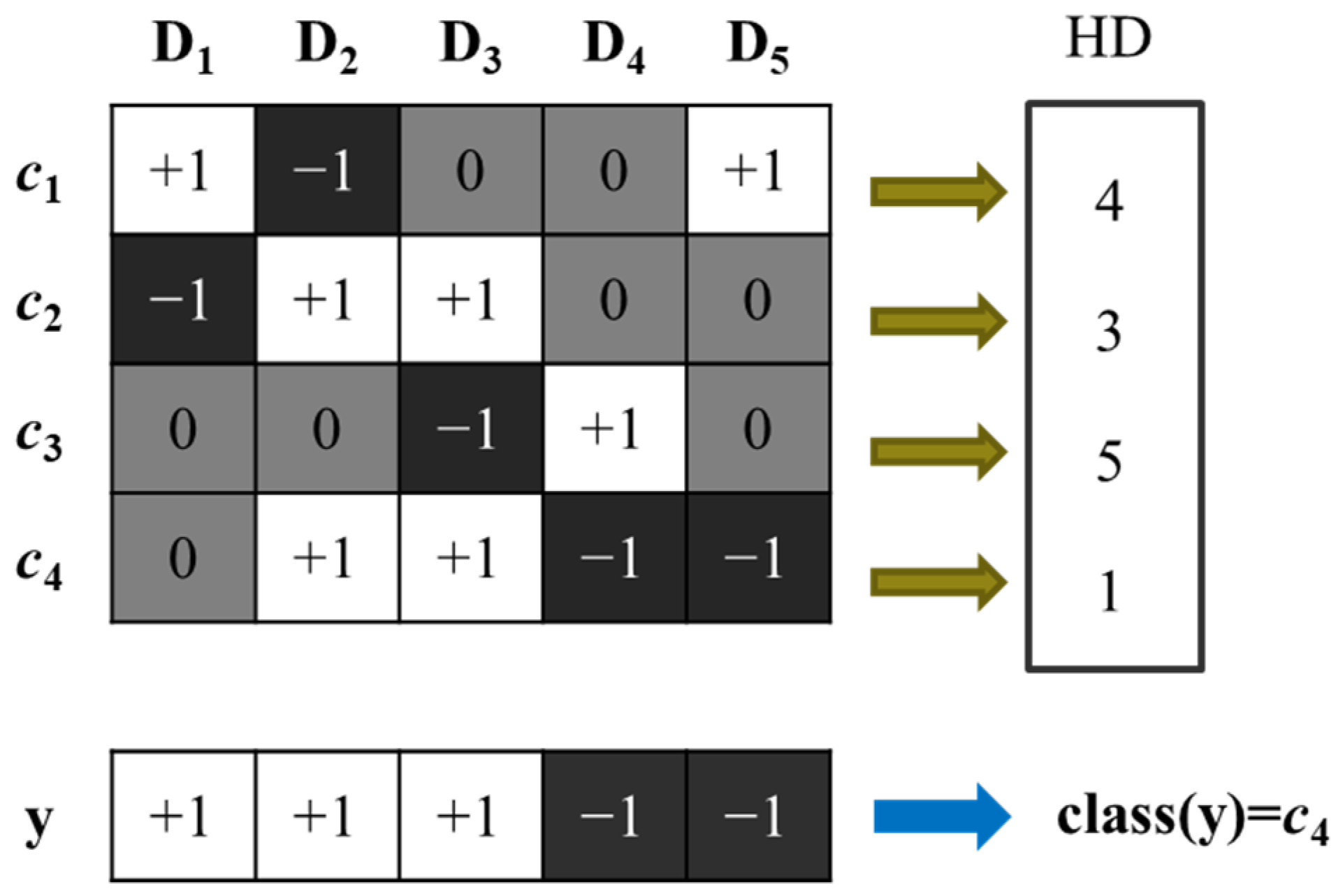
3.1.2. The Decoding Process

In the decoding process, the test sample y will get a +1 or −1 codeword under each dichotomizer, thus obtaining L codewords. Then, the Hamming distance (HD) is used to measure the distance between the code of the test sample y and the corresponding code of each class. Finally, the class corresponding to the code with the smallest distance is selected as the class to which the test sample y belongs. The formula is as follows:
class ( y ) = arg   min i = 1 , , N c   H D ( y , x i )
where xi represents the code corresponding to the i-th class, and the specific formula of HD(y,xi) is expressed as
HD ( y , x i ) = j = 1 L ( 1 sign ( y ( j ) x i ( j ) ) ) , { sign ( y ( j ) x i ( j ) ) = 1 ,   if   y ( j ) = x i ( j ) sign ( y ( j ) x i ( j ) ) = 0 ,   if   y ( j ) x i ( j )
Figure 5 visually shows the decoding process of the ECOC algorithm (taking the SR coding matrix as an example).

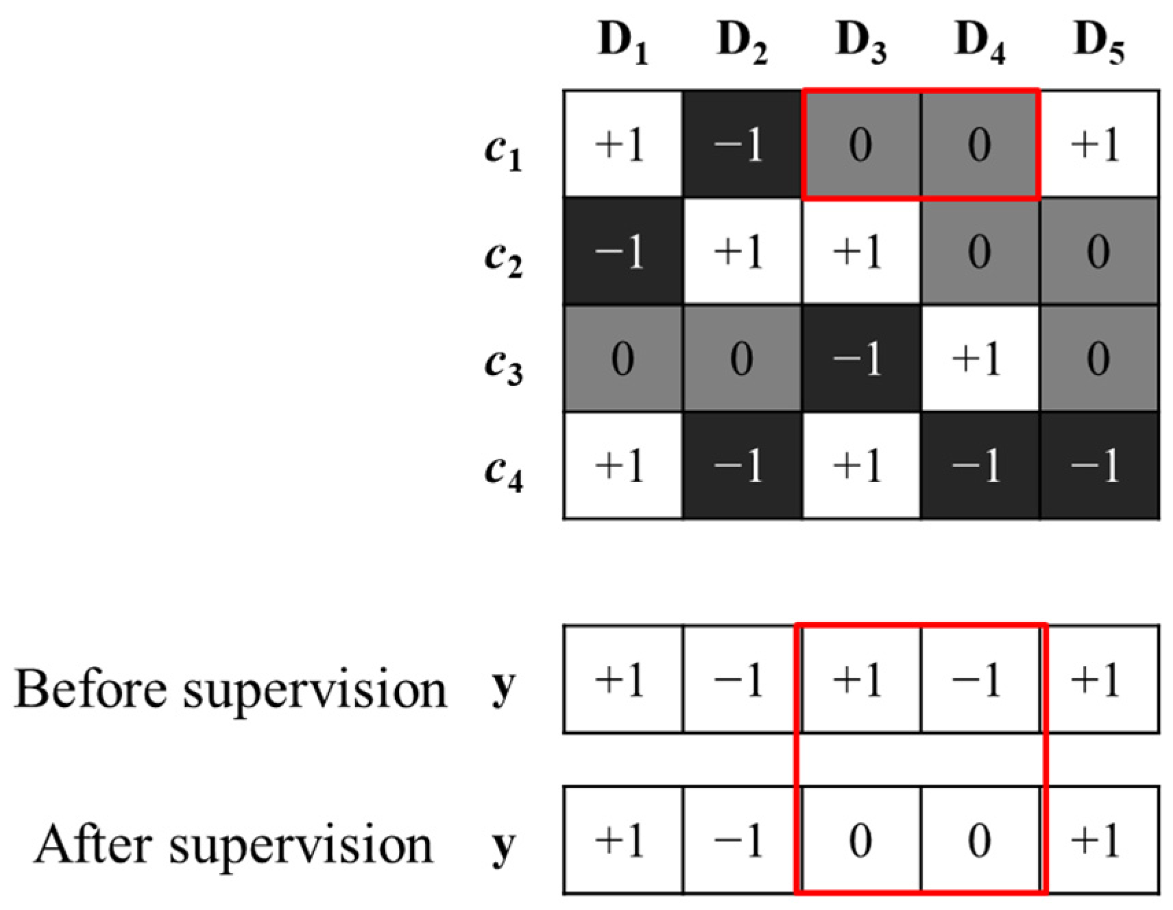
3.2. Supervision Mechanism-Based ECOC

In the SR and OVO coding matrices, the classes corresponding to the 0-element do not participate in the training process of the dichotomizer, so the trained dichotomizers are unable to recognize the classes corresponding to the 0-element. However, the test samples always get a +1 or −1 codeword under each dichotomizer, which leads to errors in the code of the test samples in the decoding process, so that the test samples may be misclassified eventually.
In this paper, aiming at the problem that 0-element in SR coding matrices affects the classification performance of ECOC, two versions of supervision-mechanism-based ECOC (SM-ECOC) algorithms are proposed, namely SM-ECOC-V1 and SM-ECOC-V2. In order to simply and intuitively express the supervision mechanism of the proposed two algorithms, the four-classification problem of the SR coding matrix is described as an example.

3.2.1. SM-ECOC-V1

The specific supervision principle of SM-ECOC-V1 is to select only the non-zero elements in the code of each class and the elements in the corresponding position of the output code of the test sample to calculate the Hamming distance in the decoding process, so as to determine the class label of the test sample. Suppose that the output code of the test sample under the dichotomizers is y = [+1, −1, +1, −1, +1], and the specific supervision process is described in Figure 6.

3.2.2. SM-ECOC-V2

The supervision mechanism of SM-ECOC-V2 is embodied in two aspects: on the one hand, it supervises the output results of the dichotomizers; on the other hand, it supervises the output codes of the test samples in the decoding process.
The process of supervising the output results of the dichotomizers is completed by a multiclass classifier, and the multiclass classifier and the ECOC algorithm independently perform the classification of the test samples. Suppose that the output code of the test sample under the dichotomizers is y = [+1, −1, +1, −1, +1], and the classification result of the test sample y under the multiclass classifier is c1. The specific supervision process is shown in Figure 7.
Firstly, the classification result c1 of the multiclass classifier is tentatively determined as the class of the test sample. Then, the dichotomizers corresponding to all 0-elements are found in the codes corresponding to class c1, namely D3 and D4. Next, the output codewords of the test sample y under dichotomizers D3 and D4 are changed to 0, as shown in the red box of Figure 7, while the output codewords of the test sample y under the other dichotomizers remain unchanged.
To further avoid the impact of 0-element on the classification performance, the SM-ECOC-V2 algorithm supervises the modified output code of the test sample again in the decoding process. As with the supervision principle of SM-ECOC-V1, only the non-zero elements in the code of each class and the elements in the corresponding position of the output code of the test sample are selected to calculate the Hamming distance, as shown in Figure 8.
The process of SM-ECOC-V2 supervising the output of dichotomizers is based on the assumption that the classification results of multiclass classifiers for test samples are correct, which requires multiclass classifiers to have good classification performance. Of course, there is no guarantee that the classification results of multiclass classifiers will be correct. Therefore, the classification results of the multiclass classifiers are not taken as the final attribution class of test samples, but the output codes of test samples under the ECOC method are modified on this basis. SM-ECOC-V2 not only reduces the influence of 0-element on the classification performance of the ECOC method, but also makes use of the error correction characteristics of ECOC, which makes this method possess good classification performance.

3.3. Selection of Base Classifier

ECOC is an ensemble learning method composed of multiple dichotomizers. In this paper, extreme learning machine (ELM) [30] is selected as the dichotomizer of ECOC, SM-ECOC-V1 and SM-ECOC-V2. Furthermore, to ensure the classification accuracy of multiclass classifier in SM-ECOC-V2, this paper adopts the ensemble classifier constructed by Bagging ensemble strategy [31] as the multiclass classifier and also selects ELM as the base classifier of Bagging ensemble classifier, called Bagging-ELM.

4. Results and Discussion

4.1. Effects of Different Seasons and Regions on Spectral Response and Classification

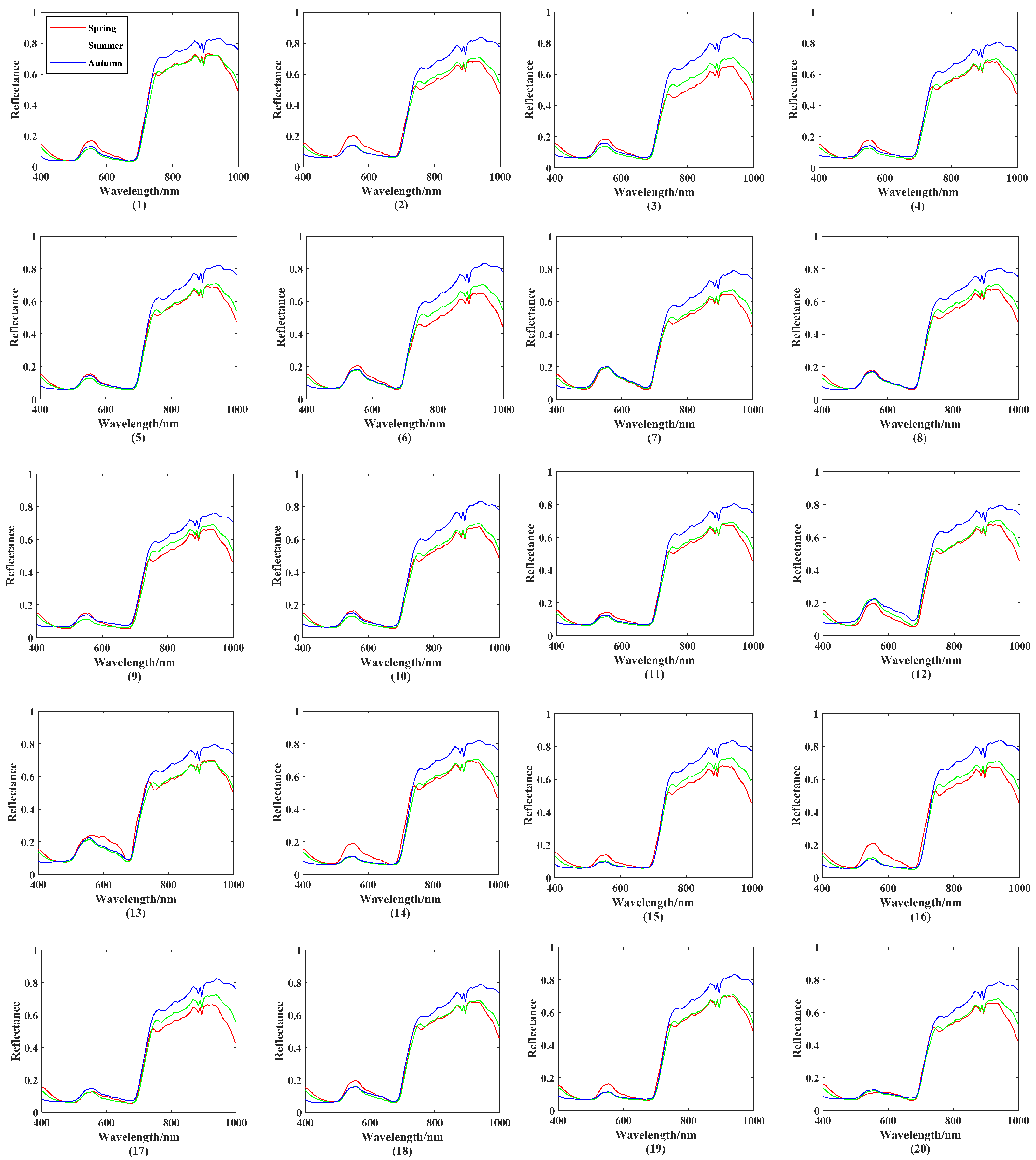
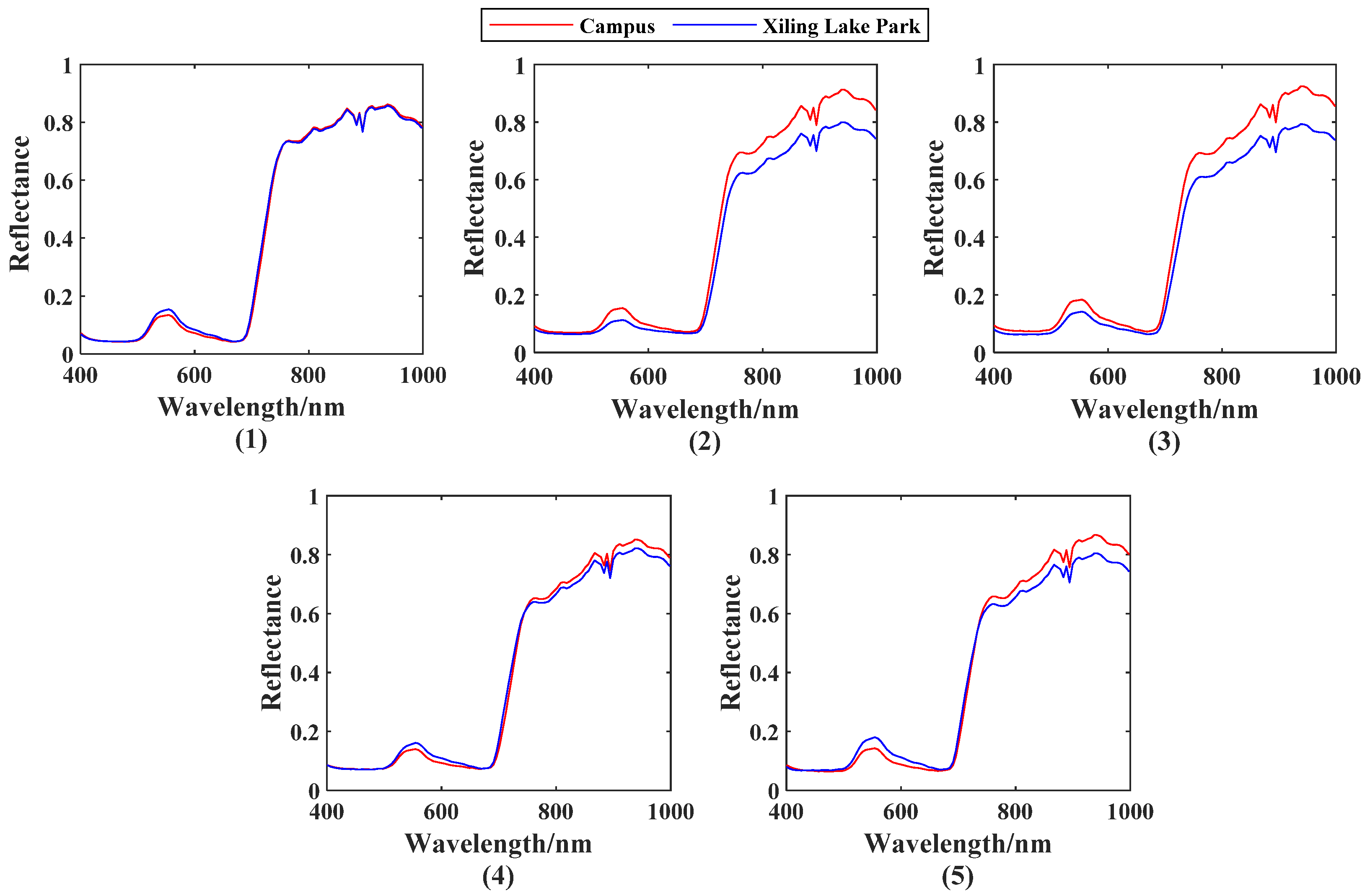
4.1.1. Hyperspectral Response Analysis of Leaves in Different Seasons and Regions

In order to analyze the influence of seasonal and regional changes on the spectral response of leaves for different tree species, the reflectance spectra of all leaf samples for each tree species in the same season or in the same region are averaged, and the average reflectance spectral data is used to represent the overall spectral response of each tree species in the same season or region.
Figure 9 shows the average reflectance spectra of leaves for 20 tree species in different seasons, in which the serial numbers of tree species correspond sequentially to those in Table 1. It can be seen from Figure 9 that the trends of reflectance spectral curves for each tree species in different seasons are basically the same, but there are differences in the reflectance level, especially in the near-infrared region of 760–1000 nm. In the near-infrared region, the spectral reflectance of the leaves for each tree species gradually increases from spring to autumn. Moreover, the spectral reflectance in autumn is significantly different from the other two seasons, while the difference between spring and summer is relatively small. In the visible-light region, the reflectance spectra of the leaves for each tree species in different seasons are significantly different in the range of 400–500 nm.
Figure 10 shows the average reflectance spectra of leaves for five tree species in different regions, in which the serial numbers of tree species correspond sequentially to those in Table 1. As seen from Figure 10, the reflectance spectral curves of leaves for each tree species in different regions also possess basically the same trend, and there are also differences in reflectance level. In the visible-light region, the reflectance spectra of the five tree species in the range of 500–600 nm are greatly affected by regional changes. In the near-infrared region of 760–1000 nm, the reflectance spectra of leaves for Lonicera maackii, Sophora japonica, Amygdalus triloba and Syringa oblata Lindl. (No. 2–5 in turn) are significantly different in different regions. However, the reflectance spectra of Ilex chinensis Sims (No. 1) are almost coincident in the near-infrared region, which indicates that the regional change produces little effect on the reflectance spectra of leaves for Ilex chinensis Sims.
In general, the reflectance spectra of leaves for various tree species will change with seasonal or regional variations. Hyperspectral technology realizes the classification of tree species through the difference of reflection spectra. However, the changes of seasons or regions will cause the change of reflection spectra of leaves for the same tree species, which will inevitably have an impact on classification of tree species.

4.1.2. Effects of Different Seasons and Regions on Tree Species Classification

To further illustrate the effects of seasonal and regional variations on tree species classification, the ELM algorithm and the samples from a single season or the same region are used to establish classification models, and these models are utilized to classify the samples from other seasons or regions, respectively. The overall accuracy (OA), class accuracy (CA), average accuracy (AA) and Kappa coefficient (Kappa) are used to comprehensively evaluate the classification effects. To avoid the omission of spectral information, the classification models are established based on all bands of original spectral data. Furthermore, to avoid any random bias, each ELM classification model is repeatedly run for 10 times under its corresponding optimal parameters, and the average of the 10 results is taken as the final classification result. The results of OA, AA and Kappa with corresponding standard deviations are shown in Table 3 and Table 4, and the results of CA are shown in Figure 11 and Figure 12.
It can be seen from Table 3 that the classification models established using samples from a single season possess very low classification accuracy when classifying the samples from other seasons, in which OA, AA and Kappa are all less than 20%. Moreover, Figure 11 shows the CA of each tree species in different seasons in detail. As can be seen from Figure 11, seasonal variations produce a serious impact on the classification of tree species, in which the CA of most tree species is less than 40%, and some species cannot even be classified at all, i.e., CA is equal to zero, such as Cerasus serrulate (No.11), Malus micromalus (No.14) and Rosa chinensis Jacq. (No.17). Furthermore, some tree species are classified with high accuracy in one season, but they are classified with very low accuracy in other seasons, such as Ilex chinensis Sims (No.1), Syringa pubescens (No.15) and Prunus Cerasifera (No.20).
Table 4 and Figure 12 shows the OA, AA and Kappa of samples from the same region classifying samples from another region and the CA of each tree species in different regions in detail, respectively. It can be seen from Table 4 that the classification models established using samples from the same region obtain very low classification accuracy when classifying the samples from other regions, in which OA, AA and Kappa are all less than 60%. Moreover, Figure 12 shows that regional variations also produce a serious impact on the classification of tree species, in which the CA of most tree species is less than 60%. Although some tree species are classified with high accuracy in one region, they are classified with very low accuracy in other regions, such as Lonicera maackii (No.2), Sophora japonica (No.3), Amygdalus triloba (No.4) and Syringa oblata Lindl. (No.5). In addition, it can be seen from Figure 12 that the CA of Ilex chinensis Sims (No.1) in different regions reaches 100%, which is mainly caused by two reasons. On the one hand, the reflectance spectra of leaves of Ilex chinensis Sims are significantly different from those of other tree species, and reflectance spectra of leaves of Ilex chinensis Sims are less affected by regional variations, which can be seen from Figure 10(1), so as to make the spectral differences among tree species obscure the spectral differences caused by regional variations. On the other hand, the established classification models only include spectral information of five tree species from different regions, which makes Ilex chinensis Sims easier to be recognized.
The above experimental results further illustrate the effects of seasonal and regional variations on tree species classification Therefore, it is necessary to consider the spectral information of season and region when establishing tree species classification models using hyperspectral technology.

4.2. Classification Performance Analysis of Supervision Mechanism-Based ECOC

To verify the superiority of the proposed SM-ECOC-V1 and SM-ECOC-V2 algorithms in this paper, the classification accuracy of these two algorithms is compared with that of tree species classification models based on all bands and feature bands established by ECOC under OVO, OVA, DR and SR four coding strategies, ELM and Bagging-ELM. In order to eliminate the effects of baseline drift, background noise and multiplicative factors caused by light condition change on spectral information, the logarithmic transformation combined with first derivative (LT-FD) method is used to preprocess the hyperspectral data of leaves before modeling.

4.2.1. Parameter Optimization

Before modeling, the parameters of each method should be optimized, so that each method can be compared in the case of optimal classification performance. Since ECOC, SM-ECOC-V1, SM-ECOC-V2 and Bagging-ELM algorithms are all ensemble algorithms, it is necessary to set the number of base classifiers for the above algorithms first.
The calculation formulas of the base classifier number for the four encoding strategies (OVO, OVA, DR and SR) of ECOC algorithm have been given in Section 3.1.1. The SM-ECOC-V1 and SM-ECOC-V2 algorithms utilize SR coding matrix, so the number of base classifiers for these two algorithms is set by the calculation formula of SR coding matrix. Because the number of tree species in this paper is 50, Nc in the formula is equal to 50. For the Bagging-ELM algorithm, there is no specific calculation formula for the number of base classifiers. In this paper, the running results of Bagging-ELM need to participate in the supervision process of SM-ECOC-V2. If the number of base classifiers for Bagging-ELM is set too large, it will not only increase its own operational complexity, but also make the operation of SM-ECOC-V2 more complex. Therefore, on the premise of ensuring the classification accuracy of Bagging-ELM, the number of base classifiers is set to 100. The number of base classifiers for each ensemble algorithm is set as shown in Table 5.
In addition, ECOC, Bagging-ELM, SM-ECOC-V1 and SM-ECOC-V2 all adopt the ELM algorithm as the base classifier. For the ELM algorithm, the number of hidden neurons has a significant effect on its classification performance. Therefore, in the framework of ECOC, Bagging-ELM, SM-ECOC-V1 and SM-ECOC-V2, the hidden neuron number of ELM is optimized, ranging from 10 to 1000 in steps of 10. In the parameter optimization process, each classifier is modeled based on all bands under each parameter, and the classification performance under each parameter is evaluated by the overall accuracy (OA). In the modeling process, 2/3 of the samples from different seasons and different regions of each tree species are randomly selected as the training set, and the rest are taken as the test set. Each classifier is repeatedly run for 10 times under each parameter, in which the training set and test set are randomly selected in each run to avoid the influence of overfitting and random errors on the OA. The average of the 10 results is taken as the final OA. After optimization, the setting of the optimal hidden neuron number for different algorithms is shown in Table 5.

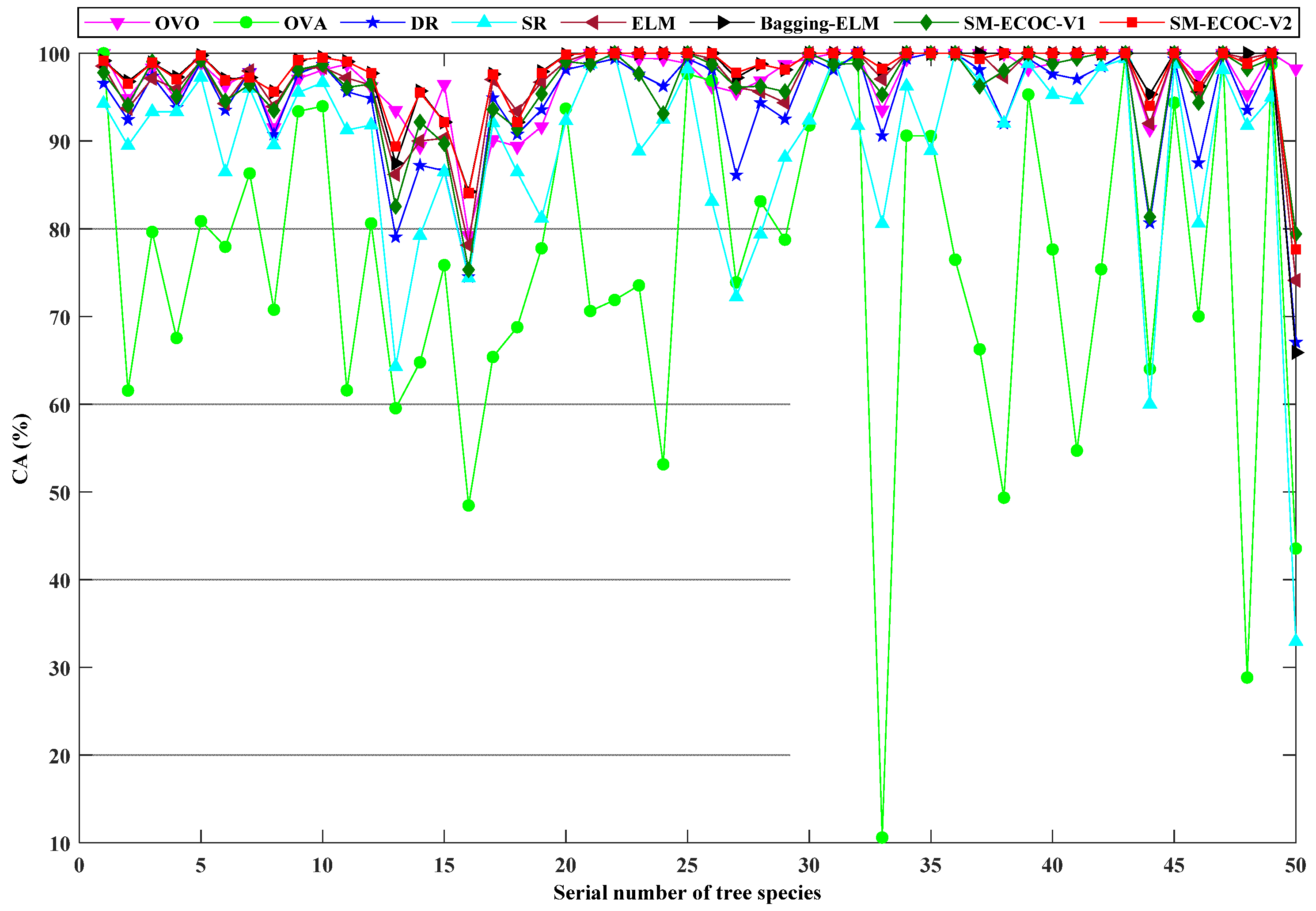
4.2.2. Classification of Tree Species Based on All Bands

The above eight algorithms are used to establish the tree species classification models based on all bands under their respective optimal parameters, and the classification performance of each model is evaluated comprehensively by OA, CA, AA and Kappa. In the process of modeling, 2/3 of the samples from different seasons and different regions of each tree species are randomly selected as the training set, and the rest are taken as the test set. In order to avoid the influence of overfitting and random errors on the classification results, each classifier is repeatedly run for 10 times under the corresponding optimal parameters, in which the training set and test set are randomly selected in each run. The average of the 10 results is taken as the final classification result. The results of OA, AA, and Kappa with corresponding standard deviations are shown in Table 6, and the results of CA are shown in Figure 13.
According to the classification results in Table 6, compared with other classification methods, the proposed SM-ECOC-V2 method achieves the best classification performance, and its OA, AA and Kappa values reach 96.98%, 97.68% and 96.88%, respectively, which are all higher than those of other methods. As seen in Figure 13, the CA values of SM-ECOC-V2 for most tree species reach more than 90% and are higher than those of other methods, in which the classification accuracy for many tree species can reach 100%. Although the CA values of SM-ECOC-V2 for some tree species are slightly lower than those of other methods, they achieve the best classification performance on the whole.
The CA values of the ECOC method based on the OVA coding strategy are lower than those of other classification methods for most tree species, and even its CA values for some tree species are less than 60%. Furthermore, the results of OA, AA and Kappa show that the classification performance of the ECOC method under the OVA encoding strategy is the worst. The reason is that OVA trains the dichotomizer by taking one of all classes as the positive class and the other classes as the negative class, which leads to the unbalanced distribution of the training samples of positive and negative class. Therefore, the classification accuracy of the trained dichotomizer for the samples of positive class will be greatly reduced.
Moreover, as seen in Table 6 and Figure 13, the classification performance of the proposed SM-ECOC-V1 and SM-ECOC-V2 methods is significantly better than that of the ECOC method under the SR coding strategy, which indicates that the supervision function of SM-ECOC-V1 and SM-ECOC-V2 methods can effectively avoid the influence of 0-element in SR coding matrix on classification performance. However, the classification performance of SM-ECOC-V1 is inferior to that of SM-ECOC-V2. From the perspective of the supervision process, compared with SM-ECOC-V2, SM-ECOC-V1 lacks the supervision for the output results of dichotomizers, but only supervises the output codes of the test samples in the decoding process. This indicates that it plays an important role in improving the classification performance of the SR coding strategy that the SM-ECOC-V2 method utilizes Bagging-ELM multiclass classifiers to supervise the output results of the dichotomizers.

4.2.3. Classification of Tree Species Based on Feature Bands

Hyperspectral data contain hundreds of bands, which provide abundant spectral information for the classification of ground objects. However, there is a high correlation between adjacent bands, making the classification accuracy increase first and then decrease with the increase of spectral bands when the number of the training samples is limited [32]. Furthermore, high-dimensional spectral data not only bring a heavy burden to the subsequent processing and calculation of data, but also cause difficulties to the transmission and storage of data [33,34]. Therefore, it is necessary to reduce the dimension of hyperspectral data.
Yang and Kan proposed a shared nearest neighbor and correlation analysis (SNNCA) method to reduce the dimension of hyperspectral data [35]. This method can select a group of feature bands with a large amount of information and low redundancy, thus avoiding the band subset falling into the local optimal solution. Therefore, this paper utilizes the SNNCA method to reduce the hyperspectral dimension, and 30 feature bands are selected to establish the tree species classification model.
As with the all-band modeling process, two out of three of the samples from different seasons and different regions of each tree species are randomly selected as the training set, and the rest are taken as the test set. Each classifier is repeatedly run for 10 times under the corresponding optimal parameters, and the average of the 10 results is taken as the final classification result. The results of OA, AA and Kappa with corresponding standard deviations are shown in Table 7, and the results of CA are shown in Figure 14.
As seen in Table 7 and Figure 14, the classification results of different methods under feature bands are similar to those under all bands. The proposed SM-ECOC-V2 method still achieves the best classification performance, with OA, AA and Kappa values of 93.89%, 95.24% and 93.70%, respectively. The CA values of SM-ECOC-V2 are also higher than those of other methods for most tree species. The results of OA, AA, CA and Kappa show that the classification performance of the ECOC method under the OVA encoding strategy is the worst, and even its CA values for some tree species are less than 60%. The specific reason has been explained in the process of analyzing the classification results under all bands.
Moreover, the classification performance of the proposed SM-ECOC-V1 and SM-ECOC-V2 methods is still significantly better than that of the ECOC method under the SR coding strategy, which further demonstrates that the supervision function of SM-ECOC-V1 and SM-ECOC-V2 methods can effectively avoid the influence of 0-element in the SR coding matrix on classification performance. The classification performance of SM-ECOC-V2 is superior to that of SM-ECOC-V1, which also further demonstrates that it plays an important role in improving the classification performance of the SR coding strategy that the SM-ECOC-V2 method utilizes Bagging-ELM multiclass classifiers to supervise the output results of the dichotomizers.

5. Conclusions

In this paper, 50 tree species were identified based on leaf hyperspectral images, in which the reflectance spectra of 20 tree species in different seasons and 5 tree species in different regions were analyzed to explore the influence of seasonal and regional changes on the hyperspectral response of tree leaves, so as to establish a hyperspectral tree species identification model suitable for different seasons and regions. Moreover, aiming at the problem that 0-element in SR coding matrices affects the classification performance of ECOC, SM-ECOC-V1 and SM-ECOC-V2 were proposed in this paper. The performance of the proposed algorithms was also compared with that of other traditional algorithms based on all bands and feature bands. The conclusions are as follows:
  • Seasonal and regional changes have an effect on the reflectance spectra of tree species, especially in the near-infrared region of 760–1000 nm. When the spectral information of different seasons and different regions is added into the model, the tree species can be effectively classified.
  • The proposed SM-ECOC-V1 and SM-ECOC-V2 methods outperform the ECOC method under SR coding strategy, which indicates that the supervision function of SM-ECOC-V1 and SM-ECOC-V2 methods can effectively avoid the influence of 0-element in SR coding matrix on classification performance.
  • The proposed SM-ECOC-V2 method achieves the best classification performance based on both all bands and feature bands, which indicates that it plays an important role in improving the classification performance of the SR coding strategy that the SM-ECOC-V2 method utilizes Bagging-ELM multiclass classifiers to supervise the output results of the dichotomizers.

Author Contributions

Data curation, R.Y.; Funding acquisition, J.K.; Investigation, R.Y.; Methodology, R.Y.; Validation, J.K.; Writing—original draft, R.Y.; Writing—review & editing, J.K. All authors have read and agreed to the published version of the manuscript.

Funding

This work was supported by the National Natural Science Foundation of China (Grant No. 32071680) and the Beijing municipal construction project special fund.

Institutional Review Board Statement

Not applicable.

Informed Consent Statement

Not applicable.

Data Availability Statement

The data supporting reported results can be obtained in the way of applying to the authors by email, without undue reservation.

Acknowledgments

We acknowledge Professor Lei Yan from Beijing Forestry University for providing hyperspectral experimental equipment, and acknowledge Beijing Forestry University and Xiling Lake Park for providing sample collection sites.

Conflicts of Interest

The authors declare no conflict of interest.

References

  1. Liu, X.S.; Zhang, X.L. Research advances and countermeasures of remote sensing classification of forest vegetation. For. Resour. Manag. 2004, 1, 61–64. [Google Scholar] [CrossRef]
  2. Zeng, Q.W.; Wu, H.G. Development of hyperspectral remote sensing application in forest species identification. For. Resour. Manag. 2009, 109–114. [Google Scholar] [CrossRef]
  3. Nevalainen, O.; Honkavaara, E.; Tuominen, S.; Viljanen, N.; Hakala, T.; Yu, X.W.; Hyyppa, J.; Saari, H.; Polonen, I.; Imai, N.N.; et al. Individual tree detection and classification with UAV-based photogrammetric point clouds and hyperspectral imaging. Remote Sens. 2017, 9, 185. [Google Scholar] [CrossRef] [Green Version]
  4. Zhang, C.M.; Mu, T.K.; Yan, T.Y.; Chen, Z.Y. Overview of hyperspectral remote sensing technology. Spacecr. Recovery Remote Sens. 2018, 39, 104–114. [Google Scholar]
  5. Zhao, C.Y.; Yang, Z.G. Technology of hyperspectral remote sensing (HRS) and its application to forest resources monitoring. For. Invent. Plan. 2006, 31, 4–6. [Google Scholar]
  6. Awad, M.M. Forest mapping: A comparison between hyperspectral and multispectral images and technologies. J. For. Res. 2018, 29, 1395–1405. [Google Scholar] [CrossRef]
  7. Mondal, B.; Saha, A.K.; Roy, A. Mapping mangroves using LISS-IV and Hyperion data in part of the Indian Sundarban. Int. J. Remote Sens. 2019, 40, 9380–9400. [Google Scholar] [CrossRef]
  8. Papes, M.; Tupayachi, R.; Martinez, P.; Peterson, A.T.; Asner, G.P.; Powell, G.V.N. Seasonal variation in spectral signatures of five genera of rainforest trees. IEEE J. Sel. Top. Appl. Earth Observ. Remote Sens. 2013, 6, 339–350. [Google Scholar] [CrossRef]
  9. Wang, L.; Fan, W.Y. Hyperspectral remote sensing data for identifying dominant forest tree species group. J. Northeast. For. Univ. 2015, 43, 134–137. [Google Scholar]
  10. Zhang, Y.N. Application of remote sensing technology in forestry. Inner Mong. For. Investig. Des. 2017, 40, 86–87. [Google Scholar]
  11. Lucas, R.; Bunting, P.; Paterson, M.; Chisholm, L. Classification of Australian forest communities using aerial photography, CASI and HyMap data. Remote Sens. Environ. 2008, 112, 2088–2103. [Google Scholar] [CrossRef]
  12. Richter, R.; Reu, B.; Wirth, C.; Doktor, D.; Vohland, M. The use of airborne hyperspectral data for tree species classification in a species-rich Central European forest area. Int. J. Appl. Earth Obs. Geoinf. 2016, 52, 464–474. [Google Scholar] [CrossRef]
  13. Tao, J.Y.; Liu, L.J.; Pang, Y.; Li, D.Q.; Feng, Y.Y.; Wang, X.; Ding, Y.L.; Peng, Q.; Xiao, W.H. Automatic identification of tree species based on air-borne LiDAR and hyperspectral data. J. Zhejiang Agric. For. Univ. 2018, 35, 314–323. [Google Scholar]
  14. Alonzo, M.; Bookhagen, B.; Roberts, D.A. Urban tree species mapping using hyperspectral and LiDAR data fusion. Remote Sens. Environ. 2014, 148, 70–83. [Google Scholar] [CrossRef]
  15. Dalponte, M.; Bruzzone, L.; Gianelle, D. Tree species classification in the Southern Alps based on the fusion of very high geometrical resolution multispectral/hyperspectral images and LiDAR data. Remote Sens. Environ. 2012, 123, 258–270. [Google Scholar] [CrossRef]
  16. Wu, Y.S.; Zhang, X.L. Object-based tree species classification using airborne hyperspectral images and LiDAR data. Forests 2020, 11, 32. [Google Scholar] [CrossRef] [Green Version]
  17. Kumar, L.; Skidmore, A.K.; Mutanga, O. Leaf level experiments to discriminate between eucalyptus species using high spectral resolution reflectance data: Use of derivatives, ratios and vegetation indices. Geocarto Int. 2010, 25, 327–344. [Google Scholar] [CrossRef]
  18. Lin, H.J.; Zhang, H.F.; Gao, Y.Q.; Li, X.; Yang, F.; Zhou, Y.F. Mahalanobis distance based hyperspectral characteristic discrimination of leaves of different desert tree species. Spectrosc. Spectr. Anal. 2014, 34, 3358–3362. [Google Scholar]
  19. Schmidt, K.S.; Skidmore, A.K. Spectral discrimination of vegetation types in a coastal wetland. Remote Sens. Environ. 2003, 85, 92–108. [Google Scholar] [CrossRef]
  20. Clark, M.L.; Roberts, D.A.; Clark, D.B. Hyperspectral discrimination of tropical rain forest tree species at leaf to crown scales. Remote Sens. Environ. 2005, 96, 375–398. [Google Scholar] [CrossRef]
  21. Castro-Esau, K.L.; Sanchez-Azofeifa, G.A.; Rivard, B.; Wright, S.J.; Quesada, M. Variability in leaf optical properties of Mesoamerican trees and the potential for species classification. Am. J. Bot. 2006, 94, 517–530. [Google Scholar] [CrossRef]
  22. Dillen, S.Y.; Op de Beeck, M.; Hufkens, K.; Buonanduci, M.; Phillips, N.G. Seasonal patterns of foliar reflectance in relation to photosynthetic capacity and color index in two co-occurring tree species, Quercus rubra and Betula papyrifera. Agric. For. Meteorol. 2012, 160, 60–68. [Google Scholar] [CrossRef]
  23. Wu, J.; Peng, J.; Wang, M.H.; Xu, J.H.; Gu, L.W. Autumn variation characteristics analysis of leaf spectrum of several common tree species. Spectrosc. Spectr. Anal. 2017, 37, 1225–1231. [Google Scholar]
  24. Zhao, X.T.; Zhang, S.J.; Liu, J.L.; Sun, H.X. Study on varieties discrimination of nectarine by hyperspectral technology combined with CARS-ELM algorithm. Mod. Food Sci. Technol. 2017, 33, 281–287. [Google Scholar]
  25. Dietterich, T.G.; Bakiri, G. Solving multiclass learning problems via error-correcting output codes. J. Artif. Intell. Res. 1995, 2, 263–286. [Google Scholar] [CrossRef] [Green Version]
  26. Dmitriev, E.V.; Kozoderov, V.V.; Dementyev, A.O.; Sokolov, A.A. Recognition of forest species and ages using algorithms based on error-correcting output codes. Eng. Technol. 2017, 10, 794–804. [Google Scholar] [CrossRef] [Green Version]
  27. Mishra, P.; Nordon, A.; Tschannerl, J.; Lian, G.P.; Redfern, S.; Marshall, S. Near-infrared hyperspectral imaging for non-destructive classification of commercial tea products. J. Food Eng. 2018, 238, 70–77. [Google Scholar] [CrossRef] [Green Version]
  28. Nazari, S.; Moin, M.S.; Kanan, H.R. Securing templates in a face recognition system using error-correcting output code and chaos theory. Comput. Electr. Eng. 2018, 72, 644–659. [Google Scholar] [CrossRef]
  29. Escalera, S.; Pujol, O.; Radeva, P. Error-correcting ouput codes library. J. Mach. Learn. Res. 2010, 11, 661–664. [Google Scholar]
  30. Huang, G.B.; Zhu, Q.Y.; Siew, C.K. Extreme learning machine: Theory and applications. Neurocomputing 2006, 70, 489–501. [Google Scholar] [CrossRef]
  31. Breiman, L. Bagging predictors. Mach. Learn. 1996, 24, 123–140. [Google Scholar] [CrossRef] [Green Version]
  32. Hughes, G. On the mean accuracy of statistical pattern recognizers. IEEE Trans. Inf. Theory 1968, 14, 55–63. [Google Scholar] [CrossRef] [Green Version]
  33. Du, Q.; Fowler, J.E.; Zhu, W. On the impact of atmospheric correction on lossy compression of multispectral and hyperspectral imagery. IEEE Trans. Geosci. Remote Sens. 2009, 47, 130–132. [Google Scholar]
  34. Yang, R.L.; Su, L.F.; Zhao, X.B.; Wan, H.; Sun, J.G. Representative band selection for hyperspectral image classification. J. Vis. Commun. Image Represent. 2017, 48, 396–403. [Google Scholar] [CrossRef]
  35. Yang, R.C.; Kan, J.M. An unsupervised hyperspectral band selection method based on shared nearest neighbor and correlation analysis. IEEE Access 2019, 7, 185532–185542. [Google Scholar] [CrossRef]
Figure 1. Collection time of samples in different seasons and regions.
Remotesensing 14 01524 g001
Figure 2. (a) The leaf image at 727.84 nm band, and (b) binary image of leaf after threshold segmentation.
Remotesensing 14 01524 g002
Figure 3. Original reflectance spectra of all leaf samples.
Remotesensing 14 01524 g003
Figure 4. Coding matrices of four coding strategies under four categories: (a) OVO, (b) OVA, (c) DR, (d) SR.
Remotesensing 14 01524 g004
Figure 5. The decoding process of ECOC algorithm.
Remotesensing 14 01524 g005
Figure 6. The output code of test sample supervised by SM-ECOC-V1 in the decoding process.
Remotesensing 14 01524 g006
Figure 7. The output results of dichotomizers supervised by SM-ECOC-V2.
Remotesensing 14 01524 g007
Figure 8. The output code of test sample supervised by SM-ECOC-V2 algorithm in the decoding process.
Remotesensing 14 01524 g008
Figure 9. Average reflectance spectra of leaves for each tree species in different seasons. (1) Ilex chinensis Sims, (2) Lonicera maackii, (3) Sophora japonica, (4) Amygdalus triloba, (5) Syringa oblata Lindl., (6) Kerria japonica, (7) Rhodotypos scandens, (8) Weigela florida, (9) Acer grosseri Pax, (10) Viburnum opulus Linn., (11) Cerasus serrulate, (12) Philadelphus pekinensis Rupr., (13) Chaenomeles speciosa, (14) Malus micromalus, (15) Syringa pubescens, (16) Ligustrum quihoui Carr., (17) Rosa chinensis Jacq., (18) Swida alba Opiz, (19) Forsythia suspensa, and (20) Prunus Cerasifera.
Remotesensing 14 01524 g009
Figure 10. Average reflectance spectra of leaves for each tree species in different regions. (1) Ilex chinensis Sims, (2) Lonicera maackii, (3) Sophora japonica, (4) Amygdalus triloba, and (5) Syringa oblata Lindl.
Remotesensing 14 01524 g010
Figure 11. Class accuracy (%) of (a) spring samples classifying summer and autumn samples, (b) summer samples classifying spring and autumn samples, and (c) autumn samples classifying spring and summer samples.
Remotesensing 14 01524 g011
Figure 12. Class accuracy (%) of (a) samples from campus classifying samples from Xiling Lake Park, and (b) samples from Xiling Lake Park classifying samples from campus.
Remotesensing 14 01524 g012
Figure 13. Class accuracy (%) of different classification models established based on all bands.
Remotesensing 14 01524 g013
Figure 14. Class accuracy (%) of different classification models established based on feature bands.
Remotesensing 14 01524 g014
Table 1. Serial number of tree species.
Serial NumberTree SpeciesSerial NumberTree SpeciesSerial NumberTree SpeciesSerial NumberTree Species
1Ilex chinensis Sims14Malus micromalus27Rosa xanthina Lindl.40Kolkwitzia amabilis Graebn.
2Lonicera maackii15Syringa pubescens28Buxus sinica41Xanthoceras sorbifolium Bunge
3Sophora japonica16Ligustrum quihoui Carr.29Cytisus scoparius42Deutzia parviflora Bge.
4Amygdalus triloba17Rosa chinensis Jacq.30Forsythia koreana‘Sun Gold’43Ginkgo biloba L.
5Syringa oblata Lindl.18Swida alba Opiz31Ligustrum vicaryi Rehder44Jasminum nudiflorum Lindl.
6Kerria japonica19Forsythia suspensa32Ulmus pumila L cv‘Jinye’45Acer truncatum Bunge
7Rhodotypos scandens20Prunus Cerasifera33Forsythia viridissima Lindl46Cercis chinensis Bunge
8Weigela florida21Syringa reticulata var. amurensis34Paeonia suffruticosa Andr.47Wisteria sinensis
9Acer grosseri Pax22Amygdalus persica L. var. persica f. duplex Rehd.35Hibiscus syriacus Linn.48Lagerstroemia indica L.
10Viburnum opulus Linn.23Pyrus xerophila36Amygdalus davidiana49Prunus persica ‘Atropurpurea’
11Cerasus serrulata24Magnolia soulangeana Soul. Bod.37Armeniaca sibirica50Berberis thunbergii var.atropurpurea Chenault
12Philadelphus pekinensis Rupr.25Zanthoxylum38Crataegus pinnatifida Bunge
13Chaenomeles speciosa26Sorbaria kirilowii39Cotoneaster multiflorus Bge.
Table 2. Equipment parameters.
Spectral RangeNumber of BandsSpectral ResolutionSize of Pixels
370–1042 nm1284.6875 nm696 × 520
Table 3. Accuracy (%) of single season samples classifying other season samples.
Training SamplesSpringSummerAutumn
Test SamplesSummerAutumnSpringAutumnSpringSummer
OA17.98 ± 3.4410.70 ± 2.7817.83 ± 2.5817.73 ± 4.227.60 ± 2.0310.35 ± 3.83
AA17.99 ± 3.5510.64 ± 2.7617.92 ± 2.5717.69 ± 4.177.64 ± 1.9810.50 ± 3.93
Kappa13.61 ± 3.656.00 ± 2.9313.51 ± 2.7213.44 ± 4.412.75 ± 2.105.71 ± 4.07
Table 4. Accuracy (%) of samples from the same region classifying samples from another region.
Training SamplesCampusXiling Lake Park
Test SamplesXiling Lake ParkCampus
OA56.01 ± 4.7958.99 ± 4.63
AA54.90 ± 4.4958.88 ± 4.61
Kappa44.33 ± 5.9948.72 ± 5.78
Table 5. The number of base classifiers and hidden neurons for different algorithms.
MethodsOVOOVADRSRELMBagging-ELMSM-ECOC-V1SM-ECOC-V2
Base classifiers1225505685No application1008585
Hidden neurons12098096069097097055080
Table 6. Accuracy (%) of different classification models established based on all bands.
MethodsOVOOVADRSRELMBagging
-ELM
SM-ECOC
-V1
SM-ECOC
-V2
OA95.71 ± 0.3875.68 ± 0.7393.52 ± 0.5589.00 ± 1.1895.60 ± 0.2196.87 ± 0.4194.93 ± 0.5296.98 ± 0.46
AA96.94 ± 0.3475.68 ± 0.7094.27 ± 0.7689.09 ± 1.1096.65 ± 0.2597.48 ± 0.4195.85 ± 0.5697.68 ± 0.46
Kappa95.58 ± 0.3974.85 ± 0.7693.32 ± 0.5688.67 ± 1.2195.46 ± 0.2196.77 ± 0.4394.77 ± 0.5396.88 ± 0.47
Table 7. Accuracy (%) of different classification models established based on feature bands.
MethodsOVOOVADRSRELMBagging
-ELM
SM-ECOC
-V1
SM-ECOC
-V2
OA92.00 ± 0.5673.58 ± 0.6390.84 ± 0.4486.45 ± 1.0593.49 ± 0.5593.74 ± 0.3892.64 ± 0.7393.89 ± 0.36
AA92.38 ± 0.6775.00 ± 1.1492.49 ± 0.5286.96 ± 1.6995.07 ± 0.6495.14 ± 0.2894.02 ± 0.7895.24 ± 0.34
Kappa91.75 ± 0.5772.67 ± 0.6690.56 ± 0.4686.03 ± 1.0893.29 ± 0.5793.54 ± 0.3992.42 ± 0.7593.70 ± 0.37
Publisher’s Note: MDPI stays neutral with regard to jurisdictional claims in published maps and institutional affiliations.

